- Title: Frequency Stability Using MPC-based Inverter Power Control in Low-Inertia Power Systems
The electrical grid is evolving from a network consisting of mostly synchronous machines to a mixture of synchronous machines and inverter-based resources such as wind, solar, and energy storage. This transformation has led to a decrease in mechanical inertia, which necessitate a need for the new resources to provide frequency responses through their inverter interfaces. In this paper we proposed a new strategy based on model predictive control to determine the optimal active-power set-point for inverters in the event of a disturbance in the system. Our framework explicitly takes the hard constraints in power and energy into account, and we show that it is robust to measurement noise, limited communications and delay by using an observer to estimate the model mismatches in real-time. We demonstrate the proposed controller significantly outperforms an optimally tuned virtual synchronous machine on a standard 39-bus system under a number of scenarios. In turn, this implies optimized inverter-based resources can provide better frequency responses compared to conventional synchronous machines.
This paper introduces a new methodology for controlling the active power of inverters in low-inertia power systems using Model Predictive Control (MPC). The electric grid is transitioning from a network dominated by synchronous machines to one that includes both synchronous machines and inverter-based resources such as wind, solar, and energy storage. This shift has led to reduced mechanical inertia, necessitating the need for new resources to provide frequency responses through their inverter interfaces.
The authors propose an MPC-based approach called MPC-Based Inverter Power Control (MIPC). MIPC aims to determine the optimal active power set-point of inverters during disturbances by simulating system dynamics over a finite horizon and optimizing these set-points. This method explicitly includes hard constraints on power and energy, providing robustness against measurement noise and communication delays.
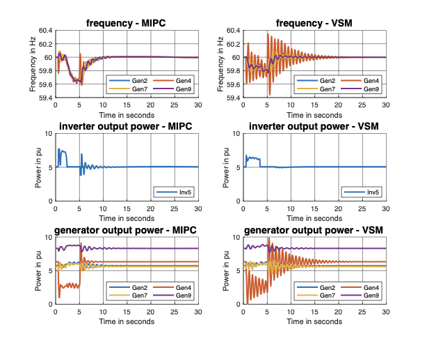
The results demonstrate that the proposed MIPC significantly outperforms optimally tuned Virtual Synchronous Machines (VSMs) in various scenarios across a standard 39-bus system, even under limited communications and large measurement noises. This study highlights the potential for optimized inverter-based resources to offer superior frequency regulation compared to conventional synchronous machines.
The electric grid has been undergoing a transition from a network with
dynamics fully governed by synchronous machines to a mixed-source
network with dynamics governed by both synchronous machines and
inverter-based resources (IBRs). This transition is marked by a
reduction in the amount of mechanical inertia in the system, which has
led to more pronounced frequency responses to disturbances and faults in
the grid . At the same time, by the virtue of the speed of power
electronic circuits, IBRs such as solar, wind and energy storage have
the capability to respond to frequency changes in the grid at a much
faster rate than traditional generators with rotating masses. The
challenge of how to best utilize these new capabilities has spurred much
research interest in the last few years (e.g., see and the references
within).
Various control strategies that utilizes the IBRs in providing frequency
regulation services has been proposed. The goal of these strategies is
to design the active power response of the IBRs to changes in frequency,
such that some frequency response objective is minimized. For example,
standard objectives of interests are the magnitude of the frequency
deviation, the rate of change of frequency (ROCOF) and the settling
time. A unique challenge in the control of IBRs is that they tend to
face much tighter limits than conventional machines. For example, solar
and wind resources cannot increase their power output beyond the maximum
power tracking point, which introduces a hard (and asymmetrical)
constraint on the action of the inverters. For a storage unit, it has
only a limited amount of energy that can be used to respond to a
disturbance.
Of the varying control strategies proposed for IBRs, Droop Control and
Virtual Synchronous Machines (VSMs) are the most popular as they
function by mimicking the frequency-power dynamic response of a
synchronous machine. As suggested by their names, droop control
injects/absorbs an amount of active power in proportion to the frequency
deviation, and VSM, in its basic configuration, acts as a second order
oscillator to provide inertia and damping to the grid. The parameters
(droop slope, inertia and damping constants) used in these strategies
can be optimized using a number of techniques .
The structural simplicity of VSMs also leads to a fundamental
limitation . Since there are only two parameters to tune (inertia and
damping) in the basic VSM configuration, there is an inherent trade-off
between different objectives and there is no choice of parameters that
will make the frequency deviation, ROCOF, and settling time small at the
same time . While the performance of the VSM can be enhanced by
incorporating virtual governors, virtual exciters and other power
systems controllers in their virtual form , it difficult to tune the
multiple parameters of the combined virtual controller simultaneously,
since the performance of one might negatively affect the other. In
addition, it is also difficult to include hard constraints, since simply
thresholding the output once the constraints are reached tend to lead to
very poor performances . Adaptive rules can be used to alleviate this
drawback somewhat, and works in change the parameter based on the
measured frequency deviation and ROCOF values. However, it is difficult
to find an optimal rule to update these parameters in real-time.
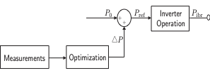
In this work, we propose a novel control strategy, based on model
predictive control (MPC), called the MPC-based Inverter Power Control
(MIPC). We explicitly formulate the problem of finding the optimal
active power set-point of an IBR to minimize the frequency deviation and
the ROCOF. It turns out that this formulation also implicitly minimizes
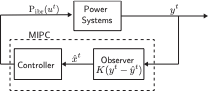
the systems settling time. More specifically, at any timestep, we
simulate the dynamics of the systems for a finite horizon, then find the
best set-points that optimizes the objective over that horizon. The
first action is then adopted for the current timestep, and the process
repeats. Our approach is similar in spirit to the ones in since an
objective is optimized in an online fashion. However, instead of
optimizing the parameters, we directly find the best power set-points.
This approach turns out to provide both an easier optimization problem
and better control performances. Namely, the hard constraints on the
IBRs are explicitly included in the optimization process.
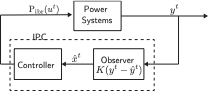
A requirement of MPC is that the IBR must have a model of the system to
be optimized. If wide-area measurements are available, then the system
states can be obtained from these measurements . In some systems, only a
limited buses are equipped with these measurement devices (e.g. PMUs).
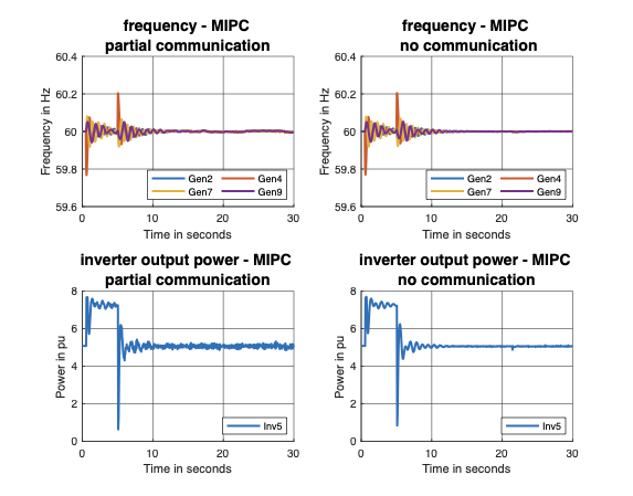
We show that our proposed MIPC framework is still applicable to these
systems by building an observer to estimate unmeasured disturbances and
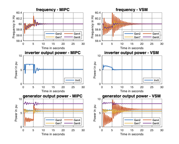
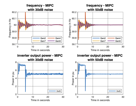
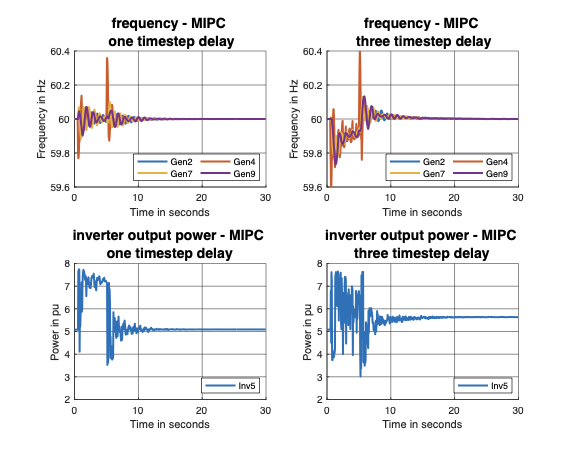
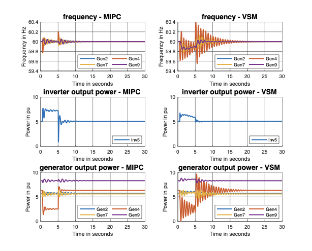
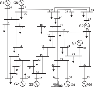
states. Through simulation studies, we show that the MIPC strictly
outperforms optimally tuned VSMs for the IEEE 39-bus system, even under
limited communication and large measurement noises.
This proposed controller finds practical application by enhancing the
capability of the IBRs to participate in providing frequency regulation
services. The additional power required can be obtained by running solar
below its maximum power point to create sufficient headroom, utilizing
the inertia from the decoupled rotating wind turbine and, leveraging on
the stored energy in a battery. By explicitly considering hard
constraints and costs on energy and power in the MPC formulation,
economic considerations can be accounted for.
The remainder of this paper is organized as follows: Section
12 defines the models used in this
paper. Section 13 presents the design and formulation
of the MIPC algorithm. Section
14 presents the state and disturbance
observer design. Section
15 compares the performances of
MIPC to VSMs in a standard test system.
Section 16 concludes the paper.
We denote the real line by $`\mathbb{R}`$, the cardinality of a set
$`\mathcal{S}`$ as $`\vert \mathcal{S} \vert`$, the $`n \times n`$
identity and zero matrices as $`\vect{I}_n`$ and $`\vect{0}_n`$,
respectively. Matrices and vectors are denoted by a bold-faced
variables.
System Structure
Steady state conditions in a power systems are achieved when there is a
balance between the power produced by the generating sources and the
power consumed by loads and lossy components. For stability analysis,
the entire system can be reduced to an equivalent network via Kron
reduction . This eliminates passive and non-dynamic load buses and
leaves only buses with at least one generating source connected. With
this in place, frequency stability analysis can be carried out, with the
frequency dynamics governed by the reactions of buses to active power
imbalances in the system.
In this work, we assume the availability of state variables and network
information for control purposes. In a later section, we will relax this
assumption to partial availability of state variables from some
generators.
Because the generators and IBRs had different dynamics, we denote their
sets by $`\mathcal{G}`$ and $`\mathcal{I}`$, respectively. Note that the
total number of generating sources in the network is
$`\mathcal{N} := \mathcal{G} \cup \mathcal{I}`$.
Synchronous Machines
The rotor dynamics of each synchronous generator in a given power system
is governed by the well-known swing equation . Here we adopt a
discretized version of the equations, which in per unit (p.u.) system
is:
\begin{equation}
 \label{eqn:swing_rotor_dis}
\begin{aligned}
\omega^{t+1}_i & = \omega^{t}_i + \frac{h}{m_i} \left(P_{\text{m},i}^t - P_{\text{e},i}^t - d_i \omega^{t}_i \right), \\
\delta^{t+1}_i & = \omega_{\text{b}} \left(\delta^{t}_i + h \ \omega^{t+1}_i\right),
\end{aligned}
\end{equation}
Click to expand and view more
$`\forall i \in \mathcal{G}`$ where $`h`$ is the step size for the
discrete simulation, $`\delta_i`$ (rad) is the rotor angle,
$`\omega = \bar{\omega}_i - \omega_0`$ is the rotor speed deviation,
$`\omega_{\text{b}}`$ is the base speed of the system, $`m_i`$ is the
inertia constant, $`d_i`$ is the damping constant, $`P_{\text{m},i}`$ is
the mechanical input power and $`P_{\text{e},i}`$ is the electric power
output of the $`i^{th}`$ machine.
The electrical output power $`P_{\text{e},i}`$ is given by the AC power
flow equation in terms of the internal emf $`\vert E_i \vert`$ and rotor
angle $`\delta_i`$:
\begin{align}
 \label{eqn:pf_dis}
P_{\text{e},i}^t = \sum_{i \sim j} \vert E_i E_j \vert [g_{ij} \cos(\delta_i^t - \delta_j^t) + b_{ij}\sin(\delta_i^t - \delta_j^t)],
\end{align}
Click to expand and view more
$`\forall i,j \in \mathcal{G}`$, where $`g_{ij} + j b_{ij}`$ is the
reduced admittance between nodes $`i`$ and $`j`$. We assume the internal
emf are constant because of the actions of the exciter systems.
The nonlinearity of the AC power flow in
[eqn:pf_dis] makes
[eqn:swing_rotor_dis] difficult
to use for control applications. Linearizing
[eqn:swing_rotor_dis] around
the nominal point and using the DC power flow approximation , the bus
dynamics become:
\begin{equation}
 \label{eqn:swing_lin_dis}
\begin{aligned}
\bigtriangleup  \omega^{t+1}_i & = \bigtriangleup  \omega^{t}_i + \frac{h}{m_i} \left(\bigtriangleup  P_{\text{m},i}^t - \bigtriangleup P_{\text{e},i}^t - d_i \bigtriangleup  \omega^{t}_i \right), \\
\bigtriangleup \delta^{t+1}_i & = \omega_{\text{b}} \left(\bigtriangleup \delta^{t}_i + h \ \bigtriangleup \omega^{t+1}_i \right),
\end{aligned}
\end{equation}
Click to expand and view more
where
$`\bigtriangleup P_{\text{e},i}^t = \sum_{i \sim j} b_{ij} \bigtriangleup \delta^t_{ij}`$
is the dc power flow between 2 buses. We model changes to the mechanical
input power $`\bigtriangleup P_{\text{m},i}^t`$ by a combination of
droop and automatic governor control (AGC) actions .
Virtual Synchronous Machine (VSM)
From the network point of view, the grid-connected IBR is seen as
producing a constant power according to its predetermined set-point and
fast dynamics governed by closed-loop controls actions . When configured
in the grid-following mode, these controls help maintain the output
power of the IBRs while remaining synchronized to the terminal voltage
set by the grid. For system analysis, the inverter can be modeled as a
voltage source behind a reactance, much like a synchronous machine.
In the event of a power imbalance in the network reflected by a
frequency deviation, an inverter does not have a “natural” response to
frequency deviation as synchronous machines does since they are made of
power electronics components and have no rotating mass. To elicit some
response, an additional control loop is therefore needed to enable the
inverters to participate in frequency control by changing the power
set-point of the inverter based on frequency measurements. The concept
of virtual synchronous machine (VSM) has been proposed in literature to
provide this additional control loop and it comes in different
configurations . The basic idea is to mimic the behavior of a
synchronous machine’s response to a frequency deviation by choosing
appropriate gains corresponding to the inertia and damping of the
machines and producing power proportional to the ROCOF and frequency
deviation. Since the response of the inverter is entirely digital, it
can be programmed with almost arbitrary functions.
In this work, we adopt the VSM configuration in , where the additional
power required to combat a frequency deviation is computed using:
\begin{equation}
 \label{eqn:p_add}
    \begin{aligned}
\bigtriangleup P = \bigtriangleup P_{\text{km}} + \bigtriangleup P_{\text{kd}}= K_\text{m} \frac{d \bigtriangleup \omega_{\text{ibr}}}{dt} + K_\text{d} \bigtriangleup \omega_{\text{ibr}}.
\end{aligned}
\end{equation}
Click to expand and view more
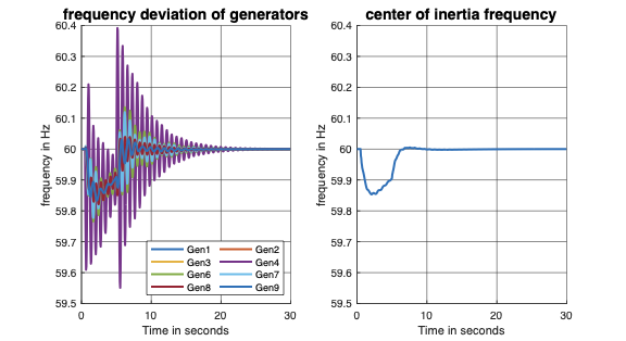
The local frequency at the IBR node
$`\bigtriangleup \omega_{\text{ibr}}`$ is approximated by the center of
inertia (COI) frequency , which is an inertia-weighted average frequency
given by:
\begin{equation}
 \label{eqn:local_freq}
    \begin{aligned}
        \bigtriangleup \omega_{ibr} = \frac{\sum_{i=1}^n m_i \bigtriangleup \omega_i}{\sum_{i=1}^n m_i}
    \end{aligned}
\end{equation}
Click to expand and view more
where $`n = \vert \mathcal{G} \vert`$, $`\bigtriangleup \omega_i`$ is
the rotor speed deviation, and $`m_i`$ is the inertia constant of the
$`i^{th}`$ synchronous generators in the network. The gains
$`K_\text{m}`$ and $`K_\text{d}`$ in
[eqn:p_add] represent the virtual inertia
and damping constants respectively. In contrast to synchronous machines
where the constants are decided by the physical parameters, these
constants of the VSM can be optimized over .
In the next section, we fully leverage the flexibility of the power
electronic interfaces using a MPC framework.
The copyright of this content belongs to the respective researchers. We deeply appreciate their hard work and contribution to the advancement of human civilization.