The DUNE Framework Core Principles and Recent Advances
📝 Original Paper Info
- Title: The DUNE Framework Basic Concepts and Recent Developments- ArXiv ID: 1909.13672
- Date: 2020-06-23
- Authors: Peter Bastian, Markus Blatt, Andreas Dedner, Nils-Arne Dreier, Christian Engwer, Ren e Fritze, Carsten Gr aser, Christoph Gr uninger, Dominic Kempf, Robert Kl ofkorn, Mario Ohlberger, Oliver Sander
📝 Abstract
This paper presents the basic concepts and the module structure of the Distributed and Unified Numerics Environment and reflects on recent developments and general changes that happened since the release of the first Dune version in 2007 and the main papers describing that state [1, 2]. This discussion is accompanied with a description of various advanced features, such as coupling of domains and cut cells, grid modifications such as adaptation and moving domains, high order discretizations and node level performance, non-smooth multigrid methods, and multiscale methods. A brief discussion on current and future development directions of the framework concludes the paper.💡 Summary & Analysis
This paper delves into the Distributed and Unified Numerics Environment (DUNE) framework, detailing its basic concepts and module structure while reflecting on recent developments since its initial release in 2007. The framework addresses several advanced features, including domain coupling techniques and cut-cell methodologies, grid modifications such as adaptation and moving domains, high-order discretizations, node-level performance enhancements, non-smooth multigrid methods, and multiscale approaches.Core Summary: This paper examines the Distributed and Unified Numerics Environment (DUNE) framework, detailing its core concepts and module structure while highlighting recent advancements since its initial release in 2007. It covers various advanced features like domain coupling techniques, grid modifications, high-order discretizations, non-smooth multigrid methods, and multiscale methodologies.
Problem Statement: The challenge is to effectively couple multiple physics simulations within complex domains using different grids while ensuring efficient integration of numerical methods for accurate results.
Solution Approach (Core Technology): DUNE provides three primary approaches. First, individual subdomains are treated separately with their own grids and interfaces are constructed between them. Second, a single host grid resolves all subdomain boundaries, where subdomain meshes are defined as subsets of the host’s elements. Third, cut-cell grids use an arbitrary host grid to construct subdomain grids by intersecting it with independent geometry representations.
Key Achievements: The DUNE framework excels in handling complex domains and integrating various numerical methods, enabling effective coupling and execution of multiple physics simulations.
Significance & Application: This research serves as a crucial tool for solving complex multiphysics problems, particularly showing significant performance improvements in high-order discretizations and parallel computing environments.
📄 Full Paper Content (ArXiv Source)
In recent years has gained support for different strategies to handle couplings of PDEs on different subdomains. One can distinguish three different approaches to describe and handle such different domains involved in a multi-physics simulation. As an important side effect, the last approach also provides support for domains with complex shapes.
-
Coupling of individual grids:
Coupling of two unrelated meshes via a merged grid: Intersecting the coupling patches yields a set of remote intersections, which can be used to evaluate the coupling conditions. In the first approach, each subdomain is treated as a separate grid, and meshed individually. The challenge is then the construction of the coupling interfaces, i.e., the geometrical relationships at common subdomain boundaries. As it is natural to construct nonconforming interfaces in this way, coupling between the subdomains will in general require some type of weak coupling, like the mortar method , penalty methods , or flux-based coupling .
-
Partition of a single grid:
 style="width:60.0%" />
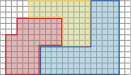
Partition of a given host mesh into subdomains. In contrast, one may construct a single host grid that resolves the boundaries of all subdomains. The subdomain meshes are then defined as subsets of elements of the host grid. While the construction of the coupling interface is straightforward, generating the initial mesh is an involved process, if the subdomains have complicated shapes. As the coupling interfaces are conforming (as long as the host grid is), it is possible to enforce coupling conditions in strong form.
-
Cut-cell grids:
 style="width:60.0%" />
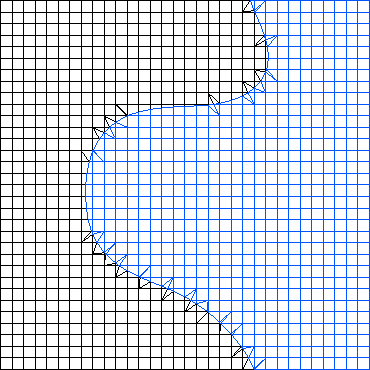
Construction of two cut-cell subdomain grids from a Cartesian background grid and a level-set geometry representation: cut-cells are constructed by intersecting a background cell with the zero-iso-surface of the level-set. The third approach is similar to the second one, and again involves a host grid. However, it is more flexible because this time the host grid can be arbitrary, and does not have to resolve the boundaries of the subdomains. Instead, subdomain grids are constructed by intersecting the elements with the independent subdomain geometry, typically described as the 0-level set of a given function. This results in so-called cut-cells, which are fragments of host grid elements. Correspondingly, the coupling interfaces are constructed by intersecting host grid elements with the subdomain boundary.
It is important to note that the shapes of the cut-cells can be arbitrary and the resulting cut-cell grids are not necessarily shape-regular. As a consequence, it is not possible to employ standard discretization techniques. Instead, a range of different methods like the unfitted discontinuous Galerkin (UDG) method and the CutFEM method have been developed for cut-cell grids.
All three concepts for handling complex domains are available as special modules.
— Coupling of individual grids
When coupling simulations on separate grids, the main challenge is the construction of coupling operators, as these require detailed neighborhood information between cells in different meshes. The module , available from https://dune-project.org/modules/dune-grid-glue , provides infrastructure to construct such relations efficiently. Neighborhood relationships are described by the concept of s, which are closely related to the s known from the module (Section 5.1.2): Both keep references to the two elements that make up the intersection, they store the shape of the intersection in world space, and the local shapes of the intersection when embedded into one or the other of the two elements. However, a is more general than its cousin: For example, the two elements do not have to be part of the same grid object, or even the same grid implementation. Also, there is no requirement for the two elements to have the same dimension. This allows mixed-dimensional couplings like the one in .
Constructing the set of remote intersections for a pair of grids first requires the selection of two coupling patches. These are two sets of entities that are known to be involved in the coupling, like a contact boundary, or the overlap between two overlapping grids. Coupling entities can have any codimension. In principle all entities of a given codimension could always be selected as coupling entities, but it is usually easy and more efficient to preselect the relevant ones.
There are several algorithms for constructing the set of remote intersections for a given pair of coupling patches. Assuming that both patches consist of roughly $`N`$ coupling entities, the naive algorithm will require $`O(N^2)`$ operations. This is too expensive for many situations. Gander and Japhet proposed an advancing front algorithm with expected linear complexity, which, however, slows down considerably when the coupling patches consist of many connected components, or contain too many entities not actually involved in the coupling. Both algorithms are available in . A third approach using a spatial data structure and a run-time of $`O(N \log N)`$ still awaits implementation.
A particular challenge arises in the case of parallel grids, as the partitioning of both grids is also unrelated. can also compute the set of in parallel codes, using additional communication. For details on the algorithm and how to handle couplings in the parallel case we refer to .
As an example we implement the assembly of mortar mass matrices using . Let $`\Omega`$ be a domain in $`\R^d`$, split into two parts $`\Omega_1`$, $`\Omega_2`$ by a hypersurface $`\Gamma`$, as in Figure 1. On $`\Omega`$ we consider an elliptic PDE for a scalar function $`u`$, subject to the continuity conditions
\begin{align*}
   u_1 & = u_2,
   \qquad
   \langle \nabla u_1, \mathbf{n} \rangle = \langle \nabla u_2, \mathbf{n} \rangle
   \qquad
   \text{on $\Gamma$},
\end{align*}where $`u_1`$ and $`u_2`$ are the restrictions of $`u`$ to the subdomains $`\Omega_1`$ and $`\Omega_2`$, respectively, and $`\mathbf{n}`$ is a unit normal of $`\Gamma`$.
For a variationally consistent discretization, the mortar methods discretizes the weak form of the continuity condition
\begin{equation}
 \label{eq:domain_decomposition:mortar_weak_continuity}
 \int_{\Omega \cap \Gamma} (u_1|_\Gamma - u_2|_\Gamma) w \, ds = 0,
\end{equation}which has to hold for a space of test functions $`w`$ defined on the common subdomain boundary. Let $`\Omega_1`$ and $`\Omega_2`$ be discretized by two independent grids, and let $`\{ \theta_i^1 \}_{i=1}^{n_1}`$ and $`\{ \theta_i^2 \}_{i=1}^{n_2}`$ be nodal basis functions for these grids, respectively. We use the nonzero restrictions of the $`\{ \theta_i^1 \}`$ on $`\Gamma`$ to discretize the test function space. Then [eq:domain_decomposition:mortar_weak_continuity] has the algebraic form
\begin{equation*}
 M_1 \overline{u}_1 - M_2 \overline{u}_2 = 0,
\end{equation*}with mortar mass matrices
\begin{alignat*}
{2}
 M_1 & \in \R^{n_{\Gamma,1} \times n_{\Gamma,1}}, & \qquad & (M_1)_{ij} = \int_{\Omega \cap \Gamma} \theta_i^1 \theta_j^1 \,ds \\
 M_2 & \in \R^{n_{\Gamma,1} \times n_{\Gamma,2}}, & \qquad & (M_2)_{ij} = \int_{\Omega \cap \Gamma} \theta_i^1 \theta_j^2 \,ds.
\end{alignat*}The numbers $`n_{\Gamma,1}`$ and $`n_{\Gamma_2}`$ denote the numbers of degrees of freedom on the interface $`\Omega \cap \Gamma`$. Assembling these matrices is not easy, because $`M_2`$ involves shape functions from two different grids.
For the implementation, assume that the grids on $`\Omega_1`$ and $`\Omega_2`$ are available as two grid view objects and , of types and , respectively. The code first constructs the coupling patches, i.e., those parts of the boundaries of $`\Omega_1`$, $`\Omega_2`$ that are on the interface $`\Gamma`$. These are represented in by objects called s. Since we are coupling on the grid boundaries—which have codimension 1—we need two s:
using Extractor1 = GridGlue::Codim1Extractor<GridView1>; using Extractor2 = GridGlue::Codim1Extractor<GridView2>;
VerticalFacetPredicate<GridView1> facetPredicate1; VerticalFacetPredicate<GridView2> facetPredicate2;
auto domEx = std::make_shared<Extractor1>(gridView1, facetPredicate1); auto tarEx = std::make_shared<Extractor2>(gridView2, facetPredicate2);
The extractors receive the information on what part of the boundary to use by two predicate objects and . Both implement a method
bool contains(const typename GridView::Traits::template Codim<0>::Entity& element, unsigned int facet) const
that returns true if the -th face of the element given in is part of the coupling boundary $`\Gamma`$. For the example we use the hyperplane $`\Gamma \subset \R^d`$ of all points with first coordinate equal to zero. Then the complete predicate class is
template <class GridView> struct VerticalFacetPredicate
bool operator()(const typename GridView::template Codim<0>::Entity& element, unsigned int facet) const
const int dim = GridView::dimension; const auto& refElement = Dune::ReferenceElements<double, dim>::general(element.type());
// Return true if all vertices of the facet // have the coordinate (numerically) equal to zero for (const auto& c : refElement.subEntities(facet,1,dim)) if ( std::abs(element.geometry().corner(c)[0] ) > 1e-6 ) return false;
return true;
;
Next, we need to compute the set of remote intersections from the two coupling patches. The different algorithms for this mentioned above are implemented in objects called “mergers”. The most appropriate one for the mortar example is called , and it implements the advancing front algorithm of Gander and Japhet. 1 The entire code to construct the remote intersections for the two trace grids at the interface $`\Gamma`$ is
using GlueType = GridGlue::GridGlue<Extractor1,Extractor2>;
// Backend for the computation of the remote intersections auto merger = std::make_shared<GridGlue::ContactMerge<dim,double> >(); GlueType gridGlue(domEx, tarEx, merger);
gridGlue.build();
The object is a container for the remote intersections. These can now be used to compute the two mass matrices $`M_1`$ and $`M_2`$. Let and be two objects of some (deliberately) unspecified matrix type. We assume that both are initialized and all entries are set to zero. The nodal bases $`\{ \theta^1_i\}_{i=1}^{n_1}`$ and $`\{ \theta^2_i\}_{i=1}^{n_2}`$ are represented by two bases. The mortar assembly loop is much like the loop for a regular mass matrix
auto nonmortarView = nonmortarBasis.localView(); auto mortarView = mortarBasis.localView();
for (const auto& intersection : intersections(gridGlue))
nonmortarView.bind(intersection.inside()); mortarView.bind(intersection.outside());
const auto& nonmortarFiniteElement = nonmortarView.tree().finiteElement(); const auto& mortarFiniteElement = mortarView.tree().finiteElement(); const auto& testFiniteElement = nonmortarView.tree().finiteElement();
// Select a quadrature rule: Use order = 2 just for simplicity int quadOrder = 2; const auto& quad = QuadratureRules<double, dim-1>::rule(intersection.type(), quadOrder);
// Loop over all quadrature points for (const auto& quadPoint : quad)
// compute integration element of overlap double integrationElement = intersection.geometry().integrationElement(quadPoint.position());
// quadrature point positions on the reference element FieldVector<double,dim> nonmortarQuadPos = intersection.geometryInInside().global(quadPoint.position()); FieldVector<double,dim> mortarQuadPos = intersection.geometryInOutside().global(quadPoint.position());
//evaluate all shapefunctions at the quadrature point std::vector<FieldVector<double,1> > nonmortarValues, mortarValues, testValues;
nonmortarFiniteElement.localBasis() .evaluateFunction(nonmortarQuadPos,nonmortarValues); mortarFiniteElement.localBasis() .evaluateFunction(mortarQuadPos,mortarValues); testFiniteElement.localBasis() .evaluateFunction(nonmortarQuadPos,testValues);
// Loop over all shape functions of the test space for (size_t i=0; i<testFiniteElement.size(); i++)
auto testIdx = nonmortarView.index(i);
// loop over all shape functions on the nonmortar side for (size_t j=0; j<nonmortarFiniteElement.localBasis().size(); j++)
auto nonmortarIdx = nonmortarView.index(j);
mortarMatrix1[testIdx][nonmortarIdx] += integrationElement * quadPoint.weight() * testValues[i] * nonmortarValues[j];
// loop over all shape functions on the mortar side for (size_t j=0; j<mortarFiniteElement.size(); j++)
auto mortarIdx = mortarView.index(j);
mortarMatrix2[testIdx][mortarIdx] += integrationElement * quadPoint.weight() * testValues[i] * mortarValues[j];
After these loops, the objects and contain the matrices $`M_1`$ and $`M_2`$, respectively.
The problem gets more complicated when $`\Gamma`$ is not a hyperplane. The approximation of a non-planar $`\Gamma`$ by unrelated grids will lead to “holes” at the interface, and the jump $`u_1|_\Gamma - u_2|_\Gamma`$ is not well-defined anymore. This situation is usually dealt with by identifying $`\Gamma_1^h`$ and $`\Gamma_2^h`$ with a homeomorphism $`\Phi`$, and replacing the second mass matrix by
\begin{equation*}
 M_2 \in \R^{n_{\Gamma,1} \times n_{\Gamma,2}},
 \qquad
 (M_2)_{ij} = \int_{\Gamma_1^h} \theta_i^2 (\theta^1_j \circ \Phi) \, ds.
\end{equation*}Only few changes have to be done to the code to implement this. First of all, the vertical predicate class has to be exchanged for something that correctly finds the curved coupling boundaries. Then, setting up extractor and objects remains unchanged. The extra magic needed to handle the mapping $`\Phi`$ is completely concealed in the implementation, which does not rely on $`\Gamma_1^h`$ and $`\Gamma_2^h`$ being identical. Instead, if there is a gap between them, a projection in normal direction is computed automatically and used for $`\Phi`$.
— Using element subsets as subdomains
The second approach to the coupling of subdomains is implemented in the module, available at https://dune-project.org/modules/dune-multidomaingrid . This module allows to structure a given host grid into different subdomains. It is implemented in terms of two cooperating grid implementations and : is a meta grid that wraps a given host grid and extends it with an interface for setting up and accessing subdomains. It also stores all data required to manage the subdomains. The individual subdomains are exposed as instances, which are lightweight objects that combine the information from the host grid and the associated . objects present a subdomain as a regular grid. A inherits all capabilities of the underlying grid, including features like $`h`$-adaptivity and MPI parallelism. Extensions of the official grid interface allow to obtain the associate entities in the fundamental mesh and the corresponding indices in both grids.
A fair share of the ideas from were incorporated in the coupling capabilities of DuMu$`^x`$ 3 .
— Assembly of cut-cell discretizations
The main challenge for cut-cell approaches is the construction of appropriate quadrature rules to evaluate integrals over the cut-cell and its boundary. We assume that the domain is given implicitly as a discrete level set function $`\Phi_h`$, s.t. $`\Phi(x) < 0`$ if $`x \in \Omega^{(i)}`$. The goal is now to compute a polygonal representation of the cut-cell and a decomposition into sub-elements, such that standard quadrature can be applied on each sub-element. This allows to evaluate weak forms on the actual domain, its boundary, and the internal skeleton (when employing DG methods).
The library implements a topology preserving marching cubes (TPMC) algorithm , assuming that $`\Phi_h`$ is given as a piecewise multilinear scalar function (i.e. a $`P^1`$ or $`Q^1`$ function). The fundamental idea in this case is the same as that of the classical marching cubes algorithm, known from computer graphics. Given the sign of the vertex values the library identifies the topology of the cut-cell. In certain ambiguous cases additional points in the interior of the cell need to be evaluated. From the topological case the actual decomposition is retrieved from a lookup table and mapped according to the real function values.
Evaluating integrals over a cut-cell domain using
We look at a simple example to learn how to work with cut-cell domains. As stated, the technical challenge regarding cut-cell methods is the construction of quadrature rules. We consider a circular domain of radius $`1`$ in 2d and compute the area using numerical quadrature. The scalar function $`\Phi : x \in \mathbb{R}^d \rightarrow |x|_2 - 1`$ describes the domain boundary as the isosurface $`\Phi = 0`$ and the interior as $`\Phi < 0`$.
using namespace Dune;
double R = 1.0; auto phi = [R](FieldVector<ctype,dim> x) return x.two_norm()-R; ;
After having setup a grid, we iterate over a given gridview , compute the $`Q_1`$ representation of $`\Phi`$ (or better to say the vertex values in an element )
double volume = 0.0; std::vector<ctype> values; for (const auto & e : elements(gv)) const auto & g = e.geometry(); // fill vertex values values.resize(g.corners()); for (std::size_t i = 0; i < g.corners(); i++) values[i] = phi(g.corner(i)); volume += localVolume(values,g);
We now compute the local volume by quadrature over the cut-cell
e$`|_{\Phi < 0}`$. In order to evaluate the integral we use the and
construct snippets, for which we can use standard quadrature rules:
template<typename Geometry> double localVolume(std::vector<double> values, const Geometry & g) double volume = 0.0; // calculate tpmc refinement TpmcRefinement<ctype,dim> refinement(values); // sum over inside domain for (const auto & snippet : refinement.volume(tpmc::InteriorDomain)) // get zero-order quadrature rule const QuadratureRule<double,dim>& quad = QuadratureRules<double,dim>::rule(snippet.type(),0); // sum over snippets for (size_t i=0; i<quad.size(); i++) volume += quad[i].weight() * snippet.integrationElement(quad[i].position()) * g.integrationElement(snippet.global(quad[i].position()));
This gives us a convergent integral, approximating $`\pi`$. Unsurprisingly we obtain an $`O(h^2)`$ convergence of the quadrature error, as the geometry is approximated as a polygonal domain.
Non-smooth multigrid
Various interesting PDEs from application fields such as computational mechanics or phase-field modeling can be written as nonsmooth convex minimization problems with certain separability properties. For such problems, the module offers an implementation of the Truncated Nonsmooth Newton Multigrid (TNNMG) algorithm .
The truncated nonsmooth Newton multigrid algorithm
TNNMG operates at the algebraic level of PDE problems. Let $`\R^N`$ be endowed with a block structure
\begin{equation*}
 \R^N = \prod_{i=1}^m \R^{N_i},
\end{equation*}and call $`R_i : \R^N \to \R^{N_i}`$ the canonical restriction to the $`i`$-th block. Typically, the factor spaces $`\R^{N_i}`$ will have small dimension, but the number of factors $`m`$ is expected to be large. A strictly convex and coercive objective functional $`J:\R^N \to \R \cup \{ \infty \}`$ is called block-separable if it has the form
\begin{align}
    \label{eq:min_problem}
    J(v) = J_0(v) + \sum_{i=1}^m \varphi_i (R_i v),
\end{align}with a convex $`C^2`$ functional $`J_0 :\R^N \to \R`$, and convex, proper, lower semi-continuous functionals $`\varphi_i : \R^{N_i} \to \R \cup \{ \infty \}`$.
Given such a functional $`J`$, the TNNMG method alternates between a nonlinear smoothing step and a damped inexact Newton correction. The smoother solves local minimization problems
\begin{align}
\label{eq:general_local_problem}
    \tilde{v}^k = \argmin_{\tilde{v} \in \tilde{v}^{k-1} + V_k} J(\tilde{v})
    \qquad
    \text{for all $k=1,\dots, m$},
\end{align}in the subspaces $`V_k \subset \R^N`$ of all vectors that have zero entries everywhere outside of the $`k`$-th block. The inexact Newton step typically consists of a single multigrid iteration for the linearized problem, but other choices are possible as well.
For this method global convergence has been shown even when using only inexact local smoothers . In practice it is observed that the method degenerates to a multigrid method after a finite number of steps, and hence multigrid convergence rates are achieved asymptotically .
The module, available from https://git.imp.fu-berlin.de/agnumpde/dune-tnnmg , offers an implementation of the TNNMG algorithm in the context of . The coupling to is very loose—as TNNMG operates on functionals in $`\R^N`$ only, there is no need for it to know about grids, finite element spaces, etc. 2 The module therefore only depends on and .
Numerical example: small-strain primal elastoplasticity
The theory of elastoplasticity describes the behavior of solid objects that can undergo both temporary (elastic) and permanent (plastic) deformation. In its simplest (primal) form, its variables are a vector field $`\mathbf{u} : \Omega \to \R^d`$ of displacements, and a matrix field $`\mathbf{p} : \Omega \to \text{Sym}^{d \times d}_0`$ of plastic strains. These strains are assumed to be symmetric and trace-free . Displacements $`\mathbf{u}`$ live in the Sobolev space $`H^1(\Omega, \R^d)`$, and (in theories without strain gradients) plastic strains live in the larger space $`L^2(\Omega, \text{Sym}^{d\times d}_0)`$. Therefore, the easiest space discretization employs continuous piecewise linear finite elements for the displacement $`\mathbf{u}`$, and piecewise constant plastic strains $`\mathbf{p}`$.
Implicit time discretization of the quasistatic model leads to a sequence of spatial problems . These can be written as minimization problems
\begin{align}
 \label{eq:algebraic_plasticity_functional}
 J(u,p)
 & \colonequals
 \frac{1}{2} (u^T \,p^T) A \begin{pmatrix} u \\ p \end{pmatrix} - b^T \begin{pmatrix} u \\ p \end{pmatrix}
 +
 \sigma_c \sum_{i=1}^{n_2} \int_\Omega \theta_i(x)\,dx \cdot \lVert p_i \rVert_F,
\end{align}which do not involve a time step size because the model is rate-independent. Here, $`u`$ and $`p`$ are the finite element coefficients of the displacement and plastic strains, respectively, and $`A`$ is a symmetric positive definite matrix. The number $`\sigma_c`$ is the yield stress, and $`b`$ is the load vector. The functions $`\theta_1,\dots, \theta_{n_2}`$ are the canonical basis functions of the space of piecewise constant functions, and $`\lVert \cdot \rVert_F : \text{Sym}^{d \times d}_0 \to \R`$ is the Frobenius norm. In the implementation, trace free symmetric matrices $`p_i \in \text{Sym}^{d \times d}_0`$ are represented by vectors of length $`\frac{1}{2}(d+1)d - 1`$.
By comparing [eq:algebraic_plasticity_functional] to [eq:min_problem], one can see that the increment functional [eq:algebraic_plasticity_functional] has the required form . By a result of , the local nonsmooth minimization problems [eq:general_local_problem] can be solved exactly.
The implementation used in employs several of the recent hybrid features of and . The pair of finite element spaces for displacements and plastic strains for a three-dimensional problem forms the tree $`(P_1)^3 \times (P_0)^5`$ (where we have identified $`\text{Sym}^{3 \times 3}_0`$ with $`\R^5`$). This tree can be constructed by
constexpr size_t nPlasticStrainComponents = dim*(dim+1)/2-1; auto plasticityBasis = makeBasis(gridView, composite( power<dim>(lagrange<1>()), // Deformation basis power<nPlasticStrainComponents>(lagrange<0>()) // Plastic strain basis ));
The corresponding linear algebra data structures must combine block vectors with block size 3 and block vectors with block size 5. Hence the vector data type definition is
using DisplacementVector = BlockVector<FieldVector<double,dim> >; using PlasticStrainVector = BlockVector< FieldVector<double,nPlasticStrainComponents> >; using Vector = MultiTypeBlockVector<DisplacementVector, PlasticStrainVector>;
and this is the type used by for the iterates. The corresponding matrix type combines four objects of different block sizes in a single , and the multigrid solver operates directly on this type of matrix.
We show a numerical example of the TNNMG solver for a three-dimensional test problem. Note that in this case, the space $`\text{Sym}^{d \times d}_0`$ is 5-dimensional, and therefore isomorphic to $`\R^5`$. Let $`\Omega`$ be the domain depicted in Figure 2, with bounding box $`(0,4) \times (0,1) \times (0,7)`$. We clamp the object at $`\Gamma_D = (0,4) \times (0,1) \times \{0\}`$, and apply a time-dependent normal load
\begin{equation*}
  \langle l(t), \bu \rangle = 20\,t \int_{\Gamma_N} \bu \cdot \be_3 \, ds
\end{equation*}on $`\Gamma_N = (0,4) \times (0,1) \times \{ 7 \}`$. The material parameters are taken from . Figure 4 shows the evolution of the plastification front at several points in time. See for more detailed numerical results and performance measurements.
Finite element spaces on discretization grids
While focuses on grid-based discretization methods for PDEs, its modular design explicitly avoids any reference to ansatz functions for discretizations in the interfaces of grids and linear algebra of the modules discussed so far. Instead of this the corresponding interfaces and implementations are contained in separate modules. However, the infrastructure is not limited to finite element discretizations and, for example, a number of applications based on the finite volume method exist, for example and the Open Porous Media Initiative , or higher order finite volume schemes on polyhedral grids as well as a tensor product multigrid approach for grids with high aspect ratios in atmospheric flows .
Local functions spaces
The core module contains interfaces and implementations for ansatz functions on local reference domains. In terms of finite element discretizations, this corresponds to the finite elements defined on reference geometries. Again following the modular paradigm, this is done independently of any global structures like grids or linear algebra, such that the module does not depend on the and module. The central concept of the module is the which is defined along the lines of a finite element in terms of . There, a finite element is a triple $`(\mathcal{D}, \Pi, \Sigma)`$ of the local domain $`\mathcal{D}`$, a local function space $`\Pi`$, and a finite set of functionals $`\Sigma=\{\sigma_1,\dots,\sigma_n\}`$ which induces a basis $`\lambda_1,\dots,\lambda_n`$ on the local ansatz space by $`\sigma_i(\lambda_j) = \delta_{ij}`$.
Each provides access to its polyhedral domain $`\mathcal{D}`$ by exporting a . The exact geometry of the type is defined in the module. The local basis functions $`\lambda_i`$ and the functionals $`\sigma_i`$ are provided by each by exporting a and object, respectively. Finally, a provides a object. The latter maps each basis function/functional to a triple $`(c,i,j)`$ which identifies the basis function as the $`j`$-th one tied to the $`i`$-th codimension-$`c`$ face of $`\mathcal{D}`$.
Global functions spaces
In contrast to local shape functions provided by , a related infrastructure for global function spaces on a grid view —denoted global finite element spaces in the following— is not contained in the core so far. Instead several concurrent/complementary discretization modules, like , , , used to provide their own implementations. To improve interoperability, an interface for global function spaces was developed as a joint effort in the staging module . This intended to be a common foundation for higher level discretization modules.
It can often be useful to use different bases of the same global finite element space for different applications. For example, a discretization in the space $`P_2`$ will often use a classical Lagrange basis of the second order polynomials on the elements, whereas hierarchical error estimators make use of the so called hierarchical $`P_2`$ basis. As a consequence the module does not use the global finite element space itself but its basis as the central abstraction. This is represented by the concept of a in the interface.
Inspired by the module, provides a flexible framework for global bases of hierarchically structured finite element product spaces. Such spaces arise, e.g. in non-isothermal phase field models, primal plasticity, mixed formulations of higher order PDEs, multi-physics problems, and many more applications. The central feature is a generic mechanism for the construction of bases for arbitrarily structured product spaces from existing elementary spaces. Within this construction, the global DOF indices can easily be customized according to the matrix/vector data structures suitable for the problem at hand, which may be flat, nested, or even multi-type containers.
In the following we will illustrate this using the $`k`$-th order Taylor–Hood space $`P_{k+1}^3 \times P_k`$ in $`\mathbb{R}^3`$ for $`k\geq 1`$ as example. Here $`P_j`$ denotes the space of $`j`$-th order continuous finite elements. Notice that the Taylor–Hood space provides a natural hierarchical structure: It is the product of the space $`P_{k+1}^3`$ for the velocity with the space $`P_k`$ for the pressure, where the former is again the 3-fold product of the space $`P_{k+1}`$ for the individual velocity components. Any such product space can be viewed as a tree of spaces, where the root denotes the full space (e.g. $`P_{k+1}^3 \times P_k`$) inner nodes denote intermediate product spaces (e.g. $`P_{k+1}^3`$), and the leaf nodes represent elementary spaces that are not considered as products themselves (e.g. $`P_{k+1}`$ and $`P_k`$).
The module on the one hand defines an interface for such nested spaces and on the other hand provides implementations for a set of elementary spaces together with a mechanism for the convenient construction of product spaces. For example, the first order Taylor–Hood space on a given grid view can be constructed using
using namespace Dune::Functions; using namespace Dune::Functions::BasisFactory; auto basis = makeBasis(gridView, composite( power<3>( lagrange<2>()), lagrange<1>()));
Here, creates a descriptor of the Lagrange basis of $`P_k`$ which is one of the pre-implemented elementary bases, creates a descriptor of an $`m`$-fold product of a given basis, and creates a descriptor of the product of an arbitrary family of (possibly different) bases. Finally, creates the global basis of the desired space on the given grid view. For other applications, and can be nested in an arbitrary way, and the mechanism can be extended by implementing further elementary spaces providing a certain implementers interface.
The interface of a is split into to several parts. All functionality that is related to the basis as a whole is directly provided by the basis, whereas all functionality that can be localized to grid elements is accessible by a so called obtained using . Binding a local view to a grid element using will then initialize (and possibly pre-compute and cache) the local properties. To avoid costly reallocation of internal data, one can rebind an existing to another element.
Once a is bound, it gives access to all non-vanishing basis functions on the bound-to element. Similar to the global basis, the localized basis forms a local tree which is accessible using . Its children can either be directly obtained using the method or traversed in a generic loop. Finally, shape functions can be accessed on each local leaf node in terms of a (cf. Section 5.3.1).
The mapping of the shape functions to global indices is done in several stages. First, the shape functions of each leaf node have unique indices within their . Next, the per- indices of each leaf node can be mapped to per- indices using . The resulting local indices enumerate all basis functions on the bound-to element uniquely. Finally, the local per- indices can be mapped to globally unique indices using . To give a full example, the global index of the $`i`$-th shape function for the $`d`$-th velocity component of the Taylor–Hood basis on a given element can be obtained using
using namespace Dune::Indices; // Use compile-time indices auto localView = basis.localView(); // Create a LocalView localView.bind(element); // Bind to a grid element auto&& velocityNode = localView.child(_0, d); // Obtain leaf node of the // d-th velocity component auto localIndex = velocityNode.localIndex(i); // Obtain local index of // i-th shape function auto globalIndex = localView.index(localIndex);// Obtain global index
Here, we made use of the compile time index because direct children in a construction may have different types.
While all local indices are flat and zero-based, global indices can in general be multi-indices which allows to efficiently access hierarchically structured containers. The global multi-indices do in general form an index tree. The latter can be explored using with a given prefix multi-index. This provides the size of the next digit following the prefix, or, equivalently, the number of direct children of the (possibly interior) node denoted by the prefix. Consistently, provides the number of entries appearing in the first digit. In case of flat indices, this corresponds to the total number of basis functions.
The way shape functions are associated to indices can be influenced according to the needs of the used discretization, algebraic data structures, and algebraic solvers. In principle an elementary basis provides a pre-defined set of global indices. When defining more complex product space bases using and , the indices provided by the respective direct children are combined in a customizable way. Possible strategies are, for example, to prepend or append the number of the child to the global index within the child, or to increment the global indices to get consecutive flat indices.
Additionally to the interfaces and implementations of global finite element function space bases, the module provides utility functions for working with global bases. The most basic utilities are , which constructs a view of only those basis functions corresponding to a certain child in the ansatz tree, , which allows to construct the finite element function (with given range type) obtained by weighting the basis functions with the coefficients stored in a suitable vector, and , which computes the interpolation of a given function storing the result as coefficient vector with respect to a basis.
The following example interpolates a function into the pressure degrees of freedom only and later construct the velocity vector field as a function. The latter can e.g. be used to write a subsampled representation in the VTK format.
// Interpolate f into vector x auto f = [] (auto x) return sin(x[0]) * sin(x[1]); ; interpolate(subspaceBasis(basis, _1), x, f); // [ Do something to compute x here ] using Range = FieldVector<double,dim>; auto velocityFunction = makeDiscreteGlobalBasisFunction<Range>(subspaceBasis(basis, _0), x);
A detailed description of the interface, the available elementary basis implementations, the mechanism to construct product spaces, the rule-based combination of global indices, and the basis-related utilities can be found in . The type-erasure based polymorphic interface of global functions and localizable grid functions as e.g. implemented by is described in .
The grid interface –
The primary object of interest when solving partial differential equations (PDEs) are functions
\begin{equation*}
f : \Omega \to R,
\end{equation*}where the domain $`\Omega`$ is a (piecewise) differentiable $`d-`$manifold embedded in $`\mathbb{R}^w`$, $`w\geq d`$, and $`R=\mathbb{R}^m`$ or $`R=\mathbb{C}^m`$ is the range. In grid-based numerical methods for the solution of PDEs the domain $`\Omega`$ is partitioned into a finite number of open, bounded, connected, and nonoverlapping subdomains $`\Omega_e`$, $`e\in E`$, $`E`$ the set of elements, satisfying
\begin{equation*}
\bigcup_{e\in E} \overline{\Omega}_e = \overline{\Omega} \qquad\text{and}\qquad
\Omega_e\cap\Omega_{e'}=\emptyset\,\text{ for $e\neq e'$}.
\end{equation*}This partitioning serves three separate but related tasks:
-
Description of the manifold. Each element $`e`$ provides a diffeomorphism (invertible and differentiable map) $`\mu_e : \hat\Omega_e \to \Omega_e`$ from its reference domain $`\hat\Omega_e\subset\mathbb{R}^d`$ to the subdomain $`\Omega_e\subset\mathbb{R}^w`$. It is assumed that the maps $`\mu_e`$ are continuous and invertible up to the boundary $`\partial\hat\Omega_e`$. Together these maps give a piecewise description of the manifold.
-
Computation of integrals. Integrals can be computed by partitioning and transformation of integrals $`\int_\Omega f(x)\,dx = \sum_{e\in E} \int_{\hat\Omega_e} f(\mu_e(\hat x)) \,d\mu_e(\hat x)`$. Typically, the reference domains $`\hat\Omega_e`$ have simple shape that is amenable to numerical quadrature.
-
Approximation of functions. Complicated functions can be approximated subdomain by subdomain for example by multivariate polynomials $`p_e(x)`$ on each subdomain $`\Omega_e`$.
The goal of is to provide a C++ interface to describe such subdivisions, from now on called a “grid”, in a generic way. Additionally, approximation of functions (Task [it:task_approximation]) requires further information to associate data with the constituents of a grid. The grid interface can handle arbitrary dimension $`d`$ (although naive grid-based methods become inefficient for larger $`d`$), arbitrary world dimension $`w`$ as well as different types of elements, local grid refinement, and parallel processing.
Grid entities and topological properties
Our aim is to separate the description of grids into a geometrical part, mainly the maps $`\mu_e`$ introduced above, and a topological part describing how the elements of the grid are constructed hierarchically from lower-dimensional objects and how the grid elements are glued together to form the grid.
The topological description can be understood recursively over the dimension $`d`$. In a one-dimensional grid, the elements are edges connecting two vertices and two neighboring elements share a common vertex. In the combinatorial description of a grid the position of a vertex is not important but the fact that two edges share a vertex is. In a two-dimensional grid the elements might be triangles and quadrilaterals which are made up of three or four edges, respectively. Elements could also be polygons with any number of edges. If the grid is conforming, neighboring elements share a common edge with two vertices or at least one vertex if adjacent.
In a three-dimensional grid elements might be tetrahedra or hexahedra consisting of triangular or quadrilateral faces, or other types up to very general polyhedra.
In order to facilitate a dimension-independent description of a grid we call its constituents entities. An entity $`e`$ has a dimension $`\dim(e)`$, where the dimension of a vertex is 0, the dimension of an edge is 1, and so on. In a $`d`$-dimensional grid the highest dimension of any entity is $`d`$ and we define the codimension of an entity as
\text{codim}(e) = d - \dim(e).We introduce the subentity relation $`\subseteq`$ with $`e'\subseteq e`$ if $`e'=e`$ or $`e'`$ is an entity contained in $`e`$, e.g. a face of a hexahedron. The set $`U(e) = \{e' : e' \subseteq e\}`$ denotes all subentities of $`e`$. The type of an entity $`\text{type}(e)`$ is characterized by the graph $`(U(e),\subseteq)`$ being isomorphic to a specific reference entity $`\hat e\in \hat E`$ (the set of all reference entities).
A $`d`$-dimensional grid is now given by all its entities $`E^c`$ of codimension $`0\leq c \leq d`$. Entities of each set $`E^c`$ are represented by a different C++ type depending on the codimension $`c`$ as a template parameter. In particular we call $`E^d`$ the set of vertices, $`E^{d-1}`$ the set of edges, $`E^{1}`$ the set of facets, and $`E^0`$ the set of elements. Grids of mixed dimension are not allowed, i.e. for every $`e'\in E^c`$, $`c>0`$ there exists $`e\in E^0`$ such that $`e'\subseteq e`$. We refer to for more details on formal properties of a grid.
provides several implementations of grids all implementing the interface. Algorithms can be written generically to operate on different grid implementations. We now provide some code snippets to illustrate the interface. First we instantiate a grid:
const int dim = 4; using Grid = Dune::YaspGrid<dim>; Dune::FieldVector<double,dim> length; for (auto& l : length) l=1.0; std::array<int,dim> nCells; for (auto& c : nCells) c=4; Grid grid(length,nCells);
Here we selected the implementation providing a $`d`$-dimensional structured, parallel grid. The dimension is set to 4 and given as a template parameter to the class. Then arguments for the constructor are prepared, which are the length of the domain per coordinate direction and the number of elements per direction. Finally, a grid object is instantiated. Construction is implementation specific. Other grid implementations might read a coarse grid from a file.
Grids can be refined in a hierarchic manner, meaning that elements are subdivided into several smaller elements. The element to be refined is kept in the grid and remains accessible. More details on local grid refinement are provided in Section 6.1 below. The following code snippet refines all elements once and then provides access to the most refined elements in a so-called :
grid.globalRefine(1); auto gv = grid.leafGridView();
A object provides read-only access to the entities of all codimensions in the view. Iterating over entities of a certain codimension is done by the following snippet using a range-based for loop:
const int codim = 2; for (const auto& e : entities(gv,Dune::Codim<codim>)) if (!e.type().isCube()) std::cout << “no cube” << std::endl;
In the loop body the type of the entity is accessed and tested for being a cube (here of dimension 2=4-2). Access via more traditional names is also possible:
for (const auto& e : elements(gv)) assert(e.codim()==0); for (const auto& e : vertices(gv)) assert(e.codim()==dim); for (const auto& e : edges(gv)) assert(e.codim()==dim-1); for (const auto& e : facets(gv)) assert(e.codim()==1);
Range-based for loops for iterating over entities have been introduced with release 2.4 in 2015. Entities of codimension 0, also called elements, provide an extended range of methods. For example it is possible to access subentities of all codimensions that are contained in a given element:
for (const auto& e : elements(gv)) for (unsigned int i=0; i<e.subEntities(codim); ++i) auto v = e.template subEntity<codim>(i);
This corresponds to iterating over $`U(e)\cap E^c`$ for a given $`e\in E^0`$.
Geometric aspects
Geometric information is provided for $`e\in E^c`$ by a map $`\mu_e : \hat\Omega_e \to \Omega_e`$, where $`\hat\Omega_e`$ is the domain associated with the reference entity $`\hat e`$ of $`e`$ and $`\Omega_e`$ is its image on the manifold $`\Omega`$. Usually $`\hat\Omega_e`$ is one of the usual shapes (simplex, cube, prism, pyramid) where numerical quadrature formulae are available. However, the grid interface also supports arbitrary polygonal elements. In that case no maps $`\mu_e`$ are provided and only the measure and the barycenter of each entity is available. Additionally, the geometry of intersections $`\Omega_e\cap\Omega_{e'}`$ with $`d-1`$-dimensional measure for $`e, e'\in E^0`$ is provided as well.
Working with geometric aspects of a grid requires working with positions, e.g. $`x\in \hat\Omega_e`$, functions, such as $`\mu_e`$, or matrices. In these follow the and interface and the most common implementations are the class templates and providing vectors and matrices with compile-time known size built on any data type having the operations of a field. Here are some examples (using dimension 3):
Dune::FieldVector<double,3> x(1.0,2.0,3.0); // construct a vector Dune::FieldVector<double,3> y(x); y *= 1.0/3.0; // scale by scalar value double s = x*y; // scalar product double norm = x.two_norm(); // compute Euclidean norm Dune::FieldMatrix<double,3,3> A(1,0,0,0,1,0,0,0,1); A.mv(x,y); // y = Ax A.usmv(0.5,x,y); // y += 0.5*Ax
An entity $`e`$ (of any codimension) offers the method returning (a reference to) a geometry object which provides, among other things, the map $`\mu_e: \hat\Omega_e\to\Omega_e`$ mapping a local coordinate in its reference domain $`\hat\Omega_e`$ to a global coordinate in $`\Omega_e`$. Additional methods provide the barycenter of $`\Omega_e`$ and the volume of $`\Omega_e`$, for example. They are used in the following code snipped to approximate the integral over a given function using the midpoint rule:
auto u = [](const auto& x)return std::exp(x.two_norm());; double integral=0.0; for (const auto& e : elements(gv)) integral += u(e.geometry().center())*e.geometry().volume();
For more accurate integration provides a variety of quadrature rules which can be selected depending on the reference element and quadrature order. Each rule is a container of quadrature points having a position and a weight. The code snippet below computes the integral over a given function with fifth order quadrature rule on any grid in any dimension. It illustrates the use of the method on the geometry which evaluates the map $`\mu_e`$ for a given (quadrature) point. The method on the geometry provides the measure arising in the transformation formula of the integral.
- double integral = 0.0; using QR =
- Dune::QuadratureRules<Grid::ctype,Grid::dimension>; for (const auto& e
- elements(gv)) auto geo = e.geometry(); const auto& quadrature = QR::rule(geo.type(),5); for (const auto& qp : quadrature) integral += u(geo.global(qp.position())) *geo.integrationElement(qp.position())*qp.weight();
An intersection $`I`$ describes the intersection $`\Omega_I = \partial\Omega_{i(I)} \cap \partial\Omega_{o(I)}`$ of two elements $`i(I)`$ and $`o(I)`$ in $`E^0`$. Intersections can be visited from each of the two elements involved. The element from which $`I`$ is visited is called the inside element $`i(I)`$ and the other one is called the outside element $`o(I)`$. Note that $`I`$ is not necessarily an entity of codimension $`1`$ in the grid. In this way allows for nonconforming grids. In a conforming grid, however, every intersection corresponds to a codimension 1 entity. For an intersection three maps are provided:
\begin{equation*}
\mu_I : \hat\Omega_I \to \Omega_I, \qquad
\eta_{I,i(I)} = \hat\Omega_I \to \hat\Omega_{i(I)}, \qquad
\eta_{I,o(I)} = \hat\Omega_I \to \hat\Omega_{o(I)} .
\end{equation*}The first map describes the domain $`\Omega_I`$ by a map from a corresponding reference element. The second two maps describe the embedding of the intersection into the reference elements of the inside and outside element, see Figure 5, such that
\begin{equation*}
\mu_I(\hat x) =  \mu_{i(I)}( \eta_{I,i(I)}(\hat x) ) = \mu_{o(I)}( \eta_{I,o(I)}(\hat x) ) .
\end{equation*}Intersections $`\Omega_I=\partial\Omega_{i(I)}\cap\partial\Omega`$ with the domain boundary are treated in the same way except that the outside element is omitted.
As an example consider the approximative computation of the elementwise divergence of a vector field $`\text{div}_e = \int_{\Omega_e} \nabla\cdot f(x) dx = \int_{\partial\Omega_e} f\cdot n ds`$ for all elements $`e\in E^0`$. Using again the midpoint rule for simplicity this is achieved by the following snippet:
auto f = [](const auto& x)return x;; for (const auto& e : elements(gv)) double divergence=0.0; for (const auto& I : intersections(gv,e)) auto geo = I.geometry(); divergence += f(geo.center())*I.centerUnitOuterNormal() *geo.volume();
Attaching data to a grid
In grid-based methods data, such as degrees of freedom in the finite element method, is associated with geometric entities and stored in containers, such as vectors, external to the grid. To that end, the grid provides an index for each entity that can be used to access random-access containers. Often there is only data for entities of a certain codimension and geometrical type (identified by its reference entity). Therefore we consider subsets of entities having the same codimension and reference entity
E^{c,\hat e} = \{ e\in E^c : \text{$e$ has reference entity $\hat e$} \}.The grid provides bijective maps
\text{index}_{c,\hat{e}} : E^{c,\hat e} \to \{0,\ldots,|E^{c,\hat e}|-1\}enumerating all the entities in $`E^{c,\hat e}`$ consecutively and starting with zero. In simple cases where only one data item is to be stored for each entity of a given codimension and geometric type this can be used directly to store data in a vector as shown in the following example:
auto& indexset = gv.indexSet(); Dune::GeometryType gt(Dune::GeometryTypes::cube(dim)); // encodes $`(c,\hat e)`$ std::vector<double> volumes(indexset.size(gt)); // allocate container for (const auto& e : elements(gv)) volumes[indexset.index(e)] = e.geometry().volume();
Here, the volumes of the elements in a single element type grid are stored in a vector. Note that a object encodes both, the dimension and the geometric type, e.g. simplex or cube. In more complicated situations an index map for entities of different codimensions and/or geometry types needs to be composed of several of the simple maps. This leaves the layout of degrees of freedom in a vector under user control and allows realization of different blocking strategies. offers several classes for this purpose, such as which can map entities of multiple codimensions and multiple geometry types to a consecutive index.
When a grid is modified through adaptive refinement, coarsening, or load balancing in the parallel case, the index maps may change as they are required to be consecutive and zero-starting. In order to store and access data reliably when the grid is modified each geometric entity is equipped with a global id:
\text{globalid} : \bigcup_{c=0}^d E^c \to \mathbb{I}where $`\mathbb{I}`$ is a set of unique identifiers. The map globalid is injective and persistent, i.e. globalid($`e`$) does not change under grid modification when entity $`e`$ is in the old and the new grid, and globalid($`e`$) is not used when $`e`$ was in the old grid and is not in the new grid (note that global ids may be used again after the next grid modification). There are very weak assuptions on the ids provided by globalid. They don’t need to be consecutive, actually they don’t even need to be numbers. Here is how element volumes would be stored in a map:
const auto& globalidset = gv.grid().globalIdSet(); using GlobalId = Grid::GlobalIdSet::IdType; std::map<GlobalId,double> volumes2; for (const auto& e : elements(gv)) volumes2[globalidset.id(e)] = e.geometry().volume();
The type represents $`\mathbb{I}`$ and must be sortable and hashable. This requirement is necessary to be able to store data for example in an or . For example, uses the class from that implements arbitrarily large unsigned integers, while uses a which is stored in each entity. In the of an element is computed from the macro element’s unique vertex ids, codimension, and refinement information.
The typical use case would be to store data in vectors and use an while the grid is in read-only state and to copy only the necessary data to a map using when the grid is being modified. Since using a may not be the most efficient way to store data, a utility class exists, that implements the strategy outlined above for arbitrary types . To allow for optimization, this class can be specialized by the grid implementation using structural information to optimize performance.
Grid refinement and coarsening
Adaptive mesh refinement using a posteriori error estimation is an established and powerful technique to reduce the computational effort in the numerical solution of PDEs, see e.g.. supports the typical estimate-mark-refine paradigm as illustrated by the following code example:
const int dim = 2; using Grid = Dune::UGGrid<dim>; auto pgrid = std::shared_ptr<Grid>( Dune::GmshReader<Grid>::read(“circle.msh”)); auto h = [](const auto& x) auto d=x.two_norm(); return 1E-6*(1-d)+0.01*d;; for (int i=0; i<15; ++i) auto gv = pgrid->leafGridView(); for (const auto& e : elements(gv)) auto diameter=std::sqrt(e.geometry().volume()/M_PI); if (diameter>h(e.geometry().center())) pgrid->mark(1,e); pgrid->preAdapt(); pgrid->adapt(); pgrid->postAdapt();
Here the implementation is used in dimension 2. In each refinement iteration those elements with a diameter larger than a desired value given by the function are marked for refinement. The method actually modifies the grid, while determines grid entities which might be deleted and clears the information about new grid entities. In between and data from the old grid needs to be stored using persistent global ids and in between and this data is transferred to the new grid. In order to identify elements that may be affected by grid coarsening and refinement the element offers two methods. The method , typically used between and , returns if the entity might vanish during the grid modifications carried out in . Afterwards, the method returns if an element was newly created during the previous call. How an element is refined when it is marked for refinement is specific to the implementation. Some implementations offer several ways to refine an element. Furthermore some grids may refine non-marked elements in an implementation specific way to ensure certain mesh properties like, e.g., conformity. For implementation of data restriction and prolongation a method provides geometrical mapping between parent and children elements.
Grid refinement is hierarchic in all currently available implementations. Each entity is associated with a grid level. After construction of a grid object all its entities are on level 0. When an entity is refined the entities resulting from this refinement, also called its direct children, are added on the next higher level. Each level-0-element and all its descendants form a tree. All entities on level $`l`$ are the entities of the level $`l`$ grid view. All entities that are not refined are the entities of the leaf grid view. This is illustrated in Figure 6. The following code snippet traverses all vertices on all levels of the grid using a :
for (int l=0; l<=pgrid->maxLevel(); l++) for (const auto& v : vertices(pgrid->levelGridView(l))) assert( v.level() == l); // check level consistency
Each provides its own and so allows to associate data with entities of a single level or with all entities in the leaf view.
Parallelization
Parallelization in is based on three concepts:
data decomposition,
message passing paradigm and
single-program-multiple-data (SPMD) style programming.
As for the refinement rules in grid adaptation the data decomposition is implementation specific but must adhere to certain rules:
-
The decomposition of codimension 0 entities $`E^0`$ into sets $`E^{0,r}`$ assigned to process rank $`r`$ form a (possibly overlapping) partitioning $`\bigcup_{i=0}^{p-1} E^{c,r} = E^c`$.
-
When process $`r`$ has a codimension 0 entity $`e`$ then it also stores all its subentities, i.e. $`e\in E^{0,r} \wedge E^c\ni f\subseteq e \Rightarrow f\in E^{c,r}`$ for $`c>0`$.
-
Each entity is assigned a partition type attribute
MATH\text{partitiontype}(e) \in \{\text{interior}, \text{border}, \text{overlap}, \text{front}, \text{ghost} \}Click to expand and view morewith the following semantics:
-
Codimension 0 entities may only have the partition types $`\text{interior}, \text{overlap}`$, or $`\text{ghost}`$. The interior codimension 0 entities $`E^{0,r,\text{interior}} = \{e\in E^{0,r} : \text{partitiontype}(e)=\text{interior}\}`$ form a nonoverlapping partitioning of $`E^0`$. Codimension 0 entities with partition type overlap can be used like regular entities whereas those with partition type ghost only provide a limited functionality (e.g. intersections may not be provided).
-
The partition type of entities with codimension $`c>0`$ is derived from the codimension 0 entities they are contained in. For any entity $`f\in E^{c}`$, $`c>0`$, set $`\Sigma^{0}(f)=\{e\in E^{0} : f\subseteq e \}`$ and $`\Sigma^{0,r}(f) = \Sigma^{0}(f) \cap E^{0,r}`$. If $`\Sigma^{0,r}(f) \subseteq E^{0,r,\text{interior}}`$ and $`\Sigma^{0,r}(f) = \Sigma^0(f)`$ then $`f`$ is interior, else if $`\Sigma^{0,r}(f) \cap E^{0,r,\text{interior}} \neq\emptyset`$ then $`f`$ is border, else if $`\Sigma^{0,r}(f)`$ contains only overlap entities and $`\Sigma^{0,r}(f) = \Sigma^0(f)`$ then $`f`$ is overlap, else if $`\Sigma^{0,r}(f)`$ contains overlap entities then $`f`$ is front, else $`f`$ is ghost.
-
Two examples of typical data decomposition models are shown in Figure 7. Variant a) on the left with interior/overlap codimension 0 entities is implemented by , variant b) on the right with the interior/ghost model is implemented by and .
To illustrate SPMD style programming we consider a simple example. Grid instantiation is done by all processes $`r`$ with identical arguments and each stores its respective grid partition $`E^{c,r}`$.
const int dim = 2; using Grid = Dune::YaspGrid<dim>; Dune::FieldVector<double,dim> length; for (auto& l:length) l=1.0; std::array<int,dim> nCells; for (auto& c : nCells) c=20; Grid grid(length,nCells,std::bitset<dim>(0ULL),1); auto gv = grid.leafGridView();
Here, the third constructor argument of the grid controls periodic boundary conditions and the last argument sets the amount of overlap in codimension 0 entities.
Parallel computation of an integral over a function using the midpoint rule is illustrated by the following code snippet:
auto u = [](const auto& x) return std::exp(x.two_norm()); ; double integral=0.0; for (const auto& e : elements(gv,Dune::Partitions::interior)) integral += u(e.geometry().center())*e.geometry().volume(); integral = gv.comm().sum(integral);
In the range-based for loop we specify in addition that iteration is restricted to interior elements. Thus, each element of the grid is visited exactly once. After each process has computed the integral on its elements a global sum (allreduce) produces the result which is now known by each process.
Data on overlapping entities $`E^{c,r}\cap E^{c,s}`$ stored by two processes $`r\neq s`$ can be communicated with the abstraction describing which information is sent for each entity and how it is processed. Communication is then initiated by the method on a . Although all current parallel grid implementation use the message passing interface (MPI) in their implementation, nowhere the user has to make explicit MPI calls. Thus, an implementation could also use shared memory access to implement the parallel functionality. Alternatively, multithreading can be used within a single process by iterating over grid entities in parallel. This has been implemented in the project or in but a common interface concept is not yet part of core functionality.
List of grid implementations
The following list gives an overview of existing implementations of the interface and their properties and the module these are implemented in. Where noted, the implementation wraps access to an external library. A complete list can be found on the web page https://dune-project.org/doc/grids/ .
Provides simplicial grids in two and three dimensions with bisection refinement based on the ALBERTA software .
Provides a parallel unstructured grid in two and three dimensions using either simplices or cubes. Refinement is nonconforming for simplices and cubes. Conforming refinement based on bisection is supported for simplices only.
Provides a parallel simplicial grid supporting curvilinear grids read from Gmsh input.
Provides an implementation of a corner point grid, a nonconforming hexahedral grid, which is the standard in the oil industry https://opm-project.org/ .
Provides one and two-dimensional grids embedded in three-dimensional space including non-manifold grids with branches .
Provides an adaptive one-dimensional grid.
A grid with polygonal cells (2d only).
Provides a parallel, unstructured grid with mixed element types (triangles and quadrilaterals in two, tetrahedra, pyramids, prisms, and hexahedra in three dimensions) and local refinement. Based on the UG library .
A parallel, structured grid in arbitrary dimension using cubes. Supports non-equidistant mesh spacing and periodic boundaries.
Metagrids use one or more implementations of the interface to provide either a new implementation of the interface or new functionality all together. Here are examples:
Takes any grid and replaces the geometries of all entities $`e`$ by the concatenation $`\mu_{geo}\circ\mu_e`$ where $`\mu_{geo}`$ is a user-defined mapping, see Section 6.1.2.
Takes any grid of dimension $`d`$ and extends it by a structured grid in direction $`d+1`$ .
Takes two grids and provides a projection of one on the other as a set of intersections , see Section 6.2.1.
Takes a grid and provides possibly overlapping sets of elements as individual grids , see Section 6.2.2.
Takes a grid and provides a subset of its entities as a new grid .
Wraps all classes of one grid implementation in new classes that delegate to the existing implementation. This can serve as an ideal base to write a new metagrid.
Takes a unstructured quadrilateral or hexahedral grid (e.g. or ) and replaces the geometry implementation with a strictly Cartesian geometry implementation for performance improvements.
Takes any grid and applies a binary filter to the entity sets for codimension $`0`$ provided by the grid view of the given grid.
A meta grid that provides the correct spherical mapping for geometries and normals for underlying spherical grids.
Major developments in the interface
Version 1.0 of the module was released on December 20, 2007. Since then a number of improvements were introduced, including the following:
-
Methods , , on and were introduced to support FV methods on polygonal and polyhedral grids.
-
provides an interface for portably creating initial meshes. uses that to import grids generated with .
-
replaced ; this allows the grid to free the memory occupied by the entity and to recreate the entity from the seed.
-
The module was introduced as a separate module to provide reference elements, geometry mappings, and quadrature formulae independent of .
-
The automatic type deduction using makes using heavily template-based libraries such as more convenient to use.
-
Initially, the interface tried to avoid copying objects for performance reasons. Many methods returned const references to internal data and disallowed copying. With copy elision becoming standard, copyable lightweight entities and intersections were introduced. Given an with codimension $`c`$ to obtain the geometry one would write:
using Geometry = typename Grid::template Codim< c >::Geometry; const Geometry& geo = entity.geometry();
whereas in newer versions one can simply write:
const auto geo = entity.geometry();
using both, the automatic type deduction and the fact that objects are copyable. A performance comparison discussing the references vs. copyable grid objects can be found in . In order to save on memory when storing entities the entity seed concept was introduced.
-
Range-based for loops for entities and intersections made iteration over grid entities very convenient. With newer versions this is simply:
for( const auto& element : Dune::elements( gridView ) ) const auto geo = element.geometry();
-
and became dune modules instead of being external libraries. This way they can be downloaded and installed like other dune modules.
As the grid interface has been adapted only slightly, it proved to work for a wide audience. Looking back, the separation of both topology and geometry, and mesh and data were good principles. Further, having entities as a view was a successful choice. Having split up in modules helped to keep the grid interface separated from other concerns. Some interface changes resulted from extensive advancements of C++11 and the subsequent standards; many are described in . Other changes turned out to make the interface easier to use or to enable different methods on top of the grid interface.
Introduction
The Distributed and Unified Numerics Environment 3 is a free and open source software framework for the grid-based numerical solution of partial differential equations (PDEs) that has been developed for more than 15 years as a collaborative effort of several universities and research institutes. In its name, the term “distributed” refers to distributed development as well as distributed computing. The enormous importance of numerical methods for PDEs in applications has lead to the development of a large number of general (i.e. not restricted to a particular application) PDE software projects. Many of them will be presented in this special issue and an incomplete list includes AMDIS , deal.II , FEniCS , FreeFEM , HiFlow , Jaumin , MFEM , Netgen/NGSolve , PETSc , and UG4 .
The distinguishing feature of in this arena is its flexibility combined with efficiency. The main goal of is to provide well-defined interfaces for the various components of a PDE solver for which then specialized implementations can be provided. is not build upon one single grid data structure or one sparse linear algebra implementation nor is the intention to focus on one specific discretization method only. All these components are meant to be exchangeable. This philosophy is based on a quote from The Mythical Man-Month: Essays on Software Engineering by Frederick Brooks :
Sometimes the strategic breakthrough will be a new algorithm, …
Much more often, strategic breakthrough will come from redoing the representation of the data or tables. This is where the heart of a program lies.
This observation has lead to the design principles of stated in :
-
Keep a clear separation of data structures and algorithms by providing abstract interfaces algorithms can be built on. Provide different, special purpose implementations of these data structures.
-
Employ generic programming using templates in C++ to remove any overhead of these abstract interfaces at compile-time. This is very similar to the approach taken by the C++ standard template library (STL).
-
Do not reinvent the wheel. This approach allows us also to reuse existing legacy code from our own and other projects in one common platform.
Another aspect of flexibility in is to structure code as much as possible into separate modules with a clear dependence.
This paper is organized as follows. In Section 4 we describe the modular structure of and the ecosystem it provides. Section 5 describes the core modules and their concepts while Section 6 describes selected advanced features and illustrates the concepts with applications. The latter section is intended for selective reading depending on the interests of the reader. Section 7 concludes the paper with current development trends in .
The Dune ecosystem
The modular structure of is implemented by conceptually splitting the code into separate, interdependent libraries. These libraries are referred to as -modules (not to be confused with C++-modules and translation units). The project offers a common infrastructure for hosting, developing, building, and testing these modules. However, modules can also be maintained independently of the official infrastructure.
The so-called core modules are maintained by the developers and each stable release provides consistent releases of all core modules. These core modules are:
Basic infrastructure for all modules such as build scripts or dense linear algebra.
Reference elements, element transformations, and quadrature rules.
Abstract interface for general grids featuring any dimension, various element types, conforming and nonconforming, local hierarchical refinement, and parallel data decomposition. Two example implementations are provided.
Abstract interfaces and implementations for sparse linear algebra and iterative solvers on matrices with small dense blocks of sizes often known at compile time.
Finite elements on the reference element.
While the core modules build a common, agreed-upon foundation for the framework, higher level functionality based on the core modules is developed by independent groups, and concurrent implementations of some features focusing on different aspects exist. These additional modules can be grouped into the following categories:
provide additional implementations of the grid interface including so-called meta grids, implementing additional functionality based on another grid implementation.
provide full-fledged implementations of finite element, finite volume, or other grid based discretization methods using the core modules. The most important ones are , , and .
provide additional functionality interesting for all users which are not yet core modules. Examples currently are Python bindings, a generic implementation of grid functions, and support for system testing.
provide frameworks for applications. They make heavy use of the features provided by the ecosystem but do not intend to merge upstream as they provide application-specific physical laws, include third-party libraries, or implement methods outside of ’s scope. Examples are the porous media simulators OPM and DuMu$`^x`$ , the FEM toolbox KASCADE7 , and the reduced basis method module -RB .
are all other modules that usually provide applications implementations for specific research projects and also new development features that are not yet used by a large number of other users but over time may become extension modules.
Some of the modules that are not part of the core are designated as so-called staging modules. These are considered to be of wider interest and may be proposed to become part of the core in the future.
The development of the software takes place on the gitlab instance (https://gitlab.dune-project.org ) where users can download and clone all openly available git repositories. They can create their own new projects, discuss issues, and open merge requests to contribute to the code base. The merge requests are reviewed by developers and others who want to contribute to the development. For each commit to the core and extension modules continuous integration tests are run to ensure code stability.
, and especially its grid interface, have proven themselves. Use cases range from personal laptops to TOP500 super computers, from mathematical and computer science methodologies to engineering application, and from bachelor thesis to research of Fortune 500 corporations.
As we laid out, ’s structure and its interfaces remained stable over the time. The modular structure of is sometimes criticized, as it might lead to different implementations to solve the same problem. We still believe that the decision was right, as it allows to experiment with new features and make them publicly available to the community without compromising the stability of the core. Other projects like FEniCS have taken similar steps. In our experience a high granularity of the software is useful.
remains under constant development and new features are added regularly. We briefly want to highlight four topics that are subject of current research and development.
Asynchronous communication
The communication overhead is expected to be an even greater problem, in future HPC systems, as the numbers of processes will increase. Therefore, it is necessary to use asynchronous communication. A first attempt to establish asynchronous communication in was demonstrated in .
With the MPI 3.0 standard, an official interface for asynchronous communication was established. Based on this standard, as part of the project, we are currently developing high-level abstractions for for such asynchronous communication, following the future-promise concept which is also used in the STL library. An object encapsulates the as well as the corresponding memory buffer. Furthermore, it provides methods to check for the state of the communication and access the result.
Thereby the fault-tolerance with respect to soft- and hard-faults that occur on remote processes is improved as well. We are following the recommended way of handling failures by throwing exceptions. Unfortunately, this concept integrates poorly with MPI. An approach how to propagate exceptions through the entire system and handle them properly, using the ULFM functionality proposed in , can be found in .
Methods like pipelined CG overlap global communication and operator application to hide communication costs. Such asynchronous solvers will be incorporated in , along with the described software infrastructure.
Thread parallelism
Modern HPC systems exhibit different levels of concurrency. Many numerical codes are now adopting the MPI+X paradigm, meaning that they use internode parallelism via MPI and intranode parallelism, i.e. threads, via some other interface. While early works where based on OpenMP and pthreads, for example in , the upcoming interface changes in will be based on the Intel Thread Building Blocks (TBB) to handle threads. Up to now the core modules don’t use multi-threading directly, but the consensus on a single library ensures interoperability among different extension modules.
In the project several numerical components like assemblers or specialized linear solvers have been developed using TBB. As many developments of are proof of concepts, these can not be merged into the core modules immediately, but we plan to port the most promising approaches to mainline . Noteworthy features include mesh partitioning into entity ranges per thread, as it is used in the MS-FEM code in Section 6.4, the block-SELL-C-$`\sigma`$ matrix format (an extension of the work of ) and a task-based DG-assembler for .
C++ and Python
Combining easy to use scripting languages with state-of-the-art numerical software has been a continuous effort in scientific computing for a long time. While much of the development of mathematical algorithms still happens in Matlab, there is increasing use of Python for such efforts, also in other scientific disciplines. For solution of PDEs the pioneering work of the FEniCS team inspired many others, e.g. to also provide Python scripting for high performance PDE solvers usually coded in C++. As discussed in Section 5.4, provides Python-bindings for central components like meshes, shape functions, and linear algebra. also provides infrastructure for exporting static polymorphic interfaces to Python using just in time compilation and without introducing a virtual layer and thus not leading to any performance losses when objects are passed between different C++ components through the Python layer. Bindings are now being added to a number of modules like the module discussed in Section 6.2.1 and further modules will follow soon.
DSLs and code-generation
Code-generation techniques allow to use scripting languages, while maintaining high efficiency. Using a domain-specific language (DSL), the FEniCS project first introduced a code generator to automatically generate efficient discretization code in Python. The Unified Form Language UFL is an embedded Python DSL for describing a PDE problem in weak form. UFL is now used by several projects, in particular Firedrake . We also started adopting this input in several places in . For example, UFL can now be used for the generating model descriptions for as demonstrated in Section 6.1. Another effort is the currently developed module, which tries to make performance optimization developed in the project accessible to the community.
In Section 6.5 we highlighted how highly tuned matrix-free higher-order kernels can achieve 40% peak performance on modern architectures. While offers the necessary flexibility, this kind of optimizations is hard to implement for average users. To overcome this issue and improve sustainability, we introduced a code generation toolchain in , using UFL as our input language. From this DSL, a header file containing a performance-optimized class is generated. The interface is ’s abstraction for local integration kernels. The design decisions for this code generation toolchain are discussed in detail in . This toolchain achieves near-optimal performance by applying structural transformations to an intermediate representation based on . A search space of SIMD vectorization strategies is explored from within the code generator through an autotuning procedure. This work now lead to the development of , which also offers other optimizations, like block-structured meshes, similar to the concepts described in , or extruded meshes, like in . This is an ongoing effort and is still in early development.
Build system and testing
Starting with the 2.4 release, has transitioned from its Autotools build system to a new, CMake-based build system. This follows the general trend in the open source software community to use CMake. The framework is split into separate modules; each module is treated as a CMake project in itself, with the build system managing inter-module dependencies and propagation of configuration results. In order to simplify the inter-module management, there is a shell script called (part of ) that resolves dependencies and controls the build order.
In the CMake implementation of the build system, special emphasis has been put on testing. Testing has become increasingly important with the development model of the core modules being heavily based on Continuous Integration. In order to lower the entrance barrier for adding tests to a minimum, a one-line solution in the form of a CMake convenience function has been implemented. Further testing infrastructure has been provided in the module , which allows the definition of system tests. These system tests describe samples of framework variability covering both compile-time and run-time variations.
More information on the CMake build system can be found in the Sphinx-generated documentation, which is available on the website4.
Grid modification
In this section we discuss two mechanisms of modifying grids within the DUNE framework: dynamic local grid adaptation and moving domains. In particular, dynamic local grid adaptation is of interest for many scientific and engineering applications due to the potential high computational cost savings. However, especially parallel dynamic local grid adaptation is technically challenging and not many PDE frameworks offer a seamless approach. We will demonstrate in this section how the general concepts described in Section 5.1 for grid views and adaptivity provided by the core modules are used to solve PDE problems on grids with dynamic refinement and coarsening. Especially important for these concepts is the separation of topology, geometry, and user data provided by the grid interface.
To support grid modification the module provides two specialized : and . Both are based on a given grid view, i.e., the , and replace certain aspects of the implementation. In the first case, the index set is replaced by an implementation that provides additional information that can be used to simplify data transfer during grid refinement and coarsening. In the second case the geometry of each element is replaced by a given grid function, e.g., by an analytic function or by some discrete function over the underlying grid view. The advantage of this meta grid view approach is that any algorithm based on a grid view can be used without change while for example the data transfer during grid modification can be transparently handled by specialized algorithms using features of the meta grid view.
Dynamic local grid adaptation
A vast number of structured or Cartesian grid managers are available
which support adaptive refinement5. There exist far fewer open source
unstructured grid managers, supporting adaptivity, for example, deal.II
which is build on top of p4est for parallel computations, or another
recent development the FEMPAR package. Both provide hexahedral grids
with non-conforming refinement. Other very capable unstructured grid
managers providing tetrahedral elements are, for example, AMDIS , FEniCS
, HiFlow , or the “Flexible Distributed Mesh Database (FMDB)” ,
libMesh , and others.
As previously described in Section 5.1.4 the grid interface offers the possibility to dynamically refine and coarsen grids if the underlying grid implementation offers these capabilities. Currently, there are two implementations that support parallel dynamic grid adaptation including load balancing, and . supports grid adaptation but cannot be used for parallel computations.
A variety of applications make use of the grid interface for adaptive computations. For example, adaptive discontinuous Galerkin computations of compressible flow, e.g. Euler equations or atmospheric flow . A number of applications focus on hp-adaptive schemes, e.g. for continuous Galerkin approximations of Poisson type problems , or discontinuous Galerkin approximations of two-phase flow in porous media or conservation laws . Other works consider, for example, the adaptive solution of the Cahn–Larché system using finite elements .
In this section we demonstrate the capabilities of the grid interface and its realizations making use of the Python bindings for the Dune module . We show only small parts of the Python code here, the full scripts are part of the tutorial .
To this end we solve the Barkley model, which is a system of reaction-diffusion equations modeling excitable media and oscillatory media. The model is often used as a qualitative model in pattern forming systems like the Belousov–Zhabotinsky reaction and other systems that are well described by the interaction of an activator and an inhibitor component .
In its simplest form the Barkley model is given by
\begin{gather*}
  \frac{\partial u}{\partial t}
       = \frac{1}{\varepsilon}f(u,v) + D\Delta u, \qquad  \frac{\partial v}{\partial t} = h(u,v),
\end{gather*}with $`f(u,v)=u\Big(1-u\Big)\Big(u-\frac{v+b}{a}\Big)`$ and $`h(u,v) = u - v`$. Finally, $`\varepsilon = 0.02`$, $`a = 0.75`$, $`b = 0.02`$, and $`D = 0.01`$ are chosen according to the web page http://www.scholarpedia.org/article/Barkley_model and . To evolve the equations in time, we employ the carefully constructed linear time stepping scheme for this model described in the literature: let $`u^n,v^n`$ be approximations of the solution at a time $`t^n`$. To compute approximations $`u^{n+1},v^{n+1}`$ at a later time $`t^{n+1}=t^n+\Delta t`$ we replace the nonlinear function $`f(u,v)`$ by $`-m(u^n,v^n)u^{n+1} + f_E(u^n,v^n)`$ where using $`U^*(V)\colonequals\frac{V+b}{a}`$
\begin{align*}
  m(U,V) &\colonequals \begin{cases}
    (U-1)\;(\;U-U^*(V)\;) & U < U^*(V) \\
    U\;(\;U-U^*(V)\;)    & U \geq U^*(V),
  \end{cases} \\
    f_E(U,V) &\colonequals \begin{cases}
    0 & U < U^*(V) \\
    U\;(\;U-U^*(V)\;)    & U \geq U^*(V).
  \end{cases}
\end{align*}Note that $`u,v`$ are assumed to be between zero and one so $`m(u^n,v^n) > 0`$. We end up with a linear, positive definite elliptic operator defining the solution $`u^{n+1}`$ given $`u^n,v^n`$. In the following we will use a conforming Lagrange approximation with quadratic basis functions. To handle possible nonconforming grids we add interior penalty DG terms as discussed in . The slow reaction $`h(u,v)`$ can be solved explicitly leading to a purely algebraic equation for $`v^{n+1}`$. The initial data is piecewise constant chosen in such a way that a spiral wave develops.
The model and initial conditions are easily provided using the Unified Form Language (UFL) . First the problem data needs to be provided
dt,t = 0.1,0 spiral_a,spiral_b,spiral_eps,spiral_D = 0.75, 0.02, 0.02, 0.01 def spiral_h(u,v): return u - v
and the discrete space and functions constructed
space = lagrange( gridView, order=2 ) x = ufl.SpatialCoordinate(space) iu = lambda s: ufl.conditional(s > 1.25, 1, 0 ) top = ufl.conditional( x[2] > 1.25,1,0) initial_u = iu(x[1])*top + iu(2.5-x[1])*(1.0 - top) initial_v = ufl.conditional(x[0]<1.25,0.5,0) uh = space.interpolate( initial_u, name=“u” ) vh = space.interpolate( initial_v, name=“v” ) uh_n, vh_n = uh.copy(), vh.copy()
Now we use UFL to describe the PDE for the function $`u`$ adding DG skeleton terms to take care of possible conforming intersections caused by local grid modification :
u, phi = ufl.TrialFunction(space), ufl.TestFunction(space) hT = ufl.MaxCellEdgeLength(space.cell()) hS = ufl.avg( ufl.MaxFacetEdgeLength(space.cell()) ) hs = ufl.MaxFacetEdgeLength(space.cell())(’+’) n = ufl.FacetNormal(space.cell()) penalty = 5 * (order * (order+1)) * spiral_D ustar = lambda v: (v+spiral_b)/spiral_a source = lambda u1,u2,u3,v: -1/spiral_eps * u1*(1-u2)*(u3-ustar(v)) # main terms xForm = inner(D_spiral*grad(u), grad(phi)) * dx xForm += ufl.conditional(uh_n<ustar(vh_n), source(u,uh_n,uh_n,vh_n), source(uh_n,u,uh_n,vh_n)) * phi * dx # dg terms xForm -= ( inner( outer(jump(u), n(’+’)), avg(spiral_D*grad(phi))) + inner( avg(spiral_D*grad(u)), outer(jump(phi), n(’+’))) ) * dS xForm += penalty/hS * inner(jump(u), jump(phi)) * dS # adding time discretization form = ( inner(u,phi) - inner(uh_n, phi) ) * dx + dt*xForm
For adaptation we use a residual based error estimator derived in for a Discontinuous Galerkin (DG) approximation for the Poisson problem. The error estimator for an element E at a given time step is given by $`\int_E \eta_E(u^{n+1}) + \frac{1}{2}\int_{\partial E}\eta_{\partial E}(u^{n+1})`$ with
\begin{align*}
  \eta_E(u_h) &= h_E^2 \Big(\frac{u_h-u^n}{\Delta t}
                 - f(u_h,v^{n+1}) + \nabla \cdot D\nabla u_h\Big)^2~, \\
  \eta_{\partial E}(u_h) &=
              h_E [\![ D\nabla u_h\cdot \nu ]\!]^2 + [\![ u_h ]\!]^2
\end{align*}where $`[\![ \cdot ]\!]`$ is the jump of the given quantity over the boundary of $`E`$ and $`\nu`$ denotes the outward unit normal. To describe the estimator using UFL we rewrite it in the form
\begin{equation*}
  R(u_h,\varphi_h) \colonequals \int_\Omega \eta_h(u_h)\varphi_h +
                      \int_{\partial\Omega} \eta_{\partial\Omega}(u_h)\{\varphi_h\}
\end{equation*}such that computing $`R(u^{n+1},\chi_E) = \int_E \eta_E(u^{n+1}) + \frac{1}{2}\int_{\partial E} \eta_{\partial E}(u^{n+1})`$ provides the estimator on each element where $`\chi_E`$ is the characteristic function on $`E`$. The characteristic functions are the basis of the finite-volume space provided by so that $`R(\cdot,\cdot)`$ can be defined using UFL as bilinear form over the solution space of $`u^{n+1}`$ and the scalar finite volume space:
fvspace = dune.fem.space.finiteVolume(uh.space.grid) estimate = fvspace.interpolate([0], name=“estimate”) chi = ufl.TestFunction(fvspace) residual = (u-uh_n)/dt - div(spiral_D*grad(u)) + source(u,u,u,vh) estimator_ufl = hT**2 * residual**2 * chi * dx + hS * inner( jump(spiral_D*grad(u)), n(’+’))**2 * avg(chi) * dS + 1/hS * jump(u)**2 * avg(chi) * dS estimator = dune.fem.operator.galerkin(estimator_ufl)
Now the grid can be modified according to the estimator within the time loop by
applying the operator constructed above to the discrete solution $`u^{n+1}`$
marking all elements where the error indicator exceeds a given tolerance for refinement and marking elements for coarsening with an indicator below a given threshold and finally
modifying the grid prolonging/restricting the data for $`u_h,v_h`$ to the new element:
estimator(uh, estimate) dune.fem.mark(estimate, maxTol,0.1*maxTol, 0,maxLevel) dune.fem.adapt([uh,vh])
where is some prescribed tolerance (in the following set to $`10^{-4}`$).
Note that only the data for $`u_h,v_h`$ is retained during the adaptation process, the underlying storage for other discrete functions used in the simulation is resized as required but the values of the functions are not maintained.
Figure 8 shows results for different times using a 2d quadrilateral grid with conforming, quadratic Lagrange basis functions. When using a conforming discrete space, the additional terms in the DG formulation vanish whenever basis functions are smooth across element intersection while these terms lead to a stabilization for nonconforming refinement/coarsening with hanging nodes. On a conforming mesh without hanging nodes the residual error estimator coincides with standard results known from the literature .
Figure 9 shows results using the quadratic Lagrange basis and a conforming simplicial grid with bisection refinement.
Figure 12 shows the same example for 3d grids, using a bi-linear Lagrange basis for a non-conforming hexahedral grid in Figure 10 and using a quadratic Lagrange basis on a conforming simplicial grid with bisection refinement in Figure 11.
Details on the available load balancing algorithms and parallel performance studies for the package can be found in , , and , and for UGGrid in .
Moving grids
In this section we touch on another important topic for modern scientific computing: moving domains. Typically this is supported by moving nodes in the computational grid. In this can be done in a very elegant way. The presence of an abstract grid interface allows the construction of meta grids where only parts of the grid implementation are re-implemented and, in addition, the original grid implementation stays untouched. Thus meta grids provide a very sophisticated way of adding features to the complete feature stack and keeping the code base modular. In one can use the meta grid (see also Section 5.1.6) which allows to move nodes of the grid by providing an overloaded implementation. Another, slightly easier way, is to only overload geometries of grid views which is, for example, done in .
Both approaches re-implement the reference geometry mapping. In an external vector of nodes providing the positions of the computational grid is used while for a grid function, i.e., a function which is evaluated on each entity given reference coordinates, is used to provide a mapping for the coordinates. The advantage of both approaches is, that the implementation of the numerical algorithm does not need to change at all. The new grid or grid view follows the same interface as the original implementation. A moving grid can now be realized by modifying this grid function.
To demonstrate this feature of we solve a mean curvature flow problem which is a specific example of a geometric evolution equation where the evolution is governed by the mean curvature $`H`$. One real-life example of this is in how soap films change over time, although it can also be applied to other problems such as image processing. Assume we are given a reference surface $`\bar\Gamma`$ such that we can write the evolving surface in the form $`\Gamma_t = X(t,\bar\Gamma)`$. It is now possible to show that the vector valued function $`X=X(t,\bar{x})`$ with $`\bar{x}\in\bar\Gamma`$ satisfies
\begin{gather*}
  \frac{\partial}{\partial t}X = - H(X)\nu(X),
\end{gather*}where $`H`$ is the mean curvature of $`\Gamma_t`$ and $`\nu`$ is its outward pointing normal.
We use the following time discrete approximation as suggest in
\begin{gather*}
  \int_{\Gamma^n} \big( U^{n+1} - x\big) \cdot \varphi\;d\sigma+
    \Delta t \int_{\Gamma^n} \nabla_{\Gamma^n} U^{n+1}
    \colon\nabla_{\Gamma^n}\varphi\;d\sigma
  =0.
\end{gather*}Here $`U^n`$ parametrizes $`\Gamma^{n+1}\approx \Gamma_{t^{n+1}}`$ over $`\Gamma^n\colonequals\Gamma_{t^{n}}`$ and $`\Delta t`$ is the time step.
In the example used here, the work flow can be set up as follows. First one creates a reference grid and a corresponding quadratic Lagrange finite element space to represent the geometry of the mapped grid.
refView = leafGridView(“sphere.dgf”, dimgrid=2, dimworld=3) refView.hierarchicalGrid.globalRefine( 2 ) space = solutionSpace(refView, dimRange=refView.dimWorld, order=2)
Then, a deformation function is projected onto this Lagrange space
x = ufl.SpatialCoordinate(space) positions = space.interpolate( x*(1 + 0.5*sin(2*pi*x[0]*x[1])*cos(pi*x[2])), name=“position”)
Using this grid function, a can be created that uses these new coordinates to represent the grid geometries. This grid view is then used to create the solution space.
gridView = geometryGridView(positions) space = lagrange(gridView, dimRange=gridView.dimWorld, order=2)
In each step of the time loop the coordinate positions can be updated, for example, by assigning the values from the computed solution of the mean curvature flow.
positions.dofVector.assign(uh.dofVector)
In Figure 13 the evolution of the surface is presented.
Other successful applications of this meta grid concept for moving domains can be found, for example, in where the compressible Navier-Stokes equations are solved in a moving domain and in where free surface shallow water flow is considered.
Python interfaces for
Combining easy to use scripting languages with state-of-the-art numerical software has been a continuous effort in scientific computing for a long time. For solution of PDEs the pioneering work of the FEniCS team inspired many others, e.g. to also provide Python scripting for high performance PDE solvers usually coded in C++.
Starting with the 2.6 release in 2018, can also be used from within the Python scripting environment. The staging module provides
a general concept for exporting realizations of polymorphic interfaces as used in many modules and
Python bindings for the central interfaces of the core modules described in this section.
These bindings make rapid prototyping of new numerical algorithms easy since they can be implemented and tested within a scripting environment. Our aim was to keep the Python interfaces as close as possible to their C++ counterparts so that translating the resulting Python algorithms to C++ to maximize efficiency of production code is as painless as possible. Bindings are provided using .
We start with an example demonstrating these concepts. We revisit the examples given in Section 5.1.1 starting with the construction of a simple Cartesian grid in four space dimensions and the approximation of the integral of a function over that grid. The corresponding Python code is
from dune.grid import yaspGrid, cartesianDomain from math import exp dim = 4 lower = 4*[0.] upper = 4*[1.] nCells = 4*[4] gv = yaspGrid(constructor=cartesianDomain(lower,upper,nCells)) u = lambda x: exp(x.two_norm) integral = 0.0 for e in gv.elements: integral += u(e.geometry.center)*e.geometry.volume
A few changes were made to make the resulting code more Pythonic, i.e., the use of class attributes instead of class methods, but the only major change is that the function returning the grid object in fact returns the leaf grid view and not the hierarchic grid structure. Notice that the life time of this underlying grid is managed automatically by Python’s internal reference counting mechanism. It can be obtained using a class attribute, i.e., to refine the grid globally
gv.hierarchicalGrid.globalRefine(1);
Other interface classes and their realizations have also been exported so that for example the more advanced quadrature rules used in the previous sections can also be used in Python:
from dune.geometry import quadratureRule integral = 0.0 for e in gv.elements: geo = e.geometry quadrature = quadratureRule(e.type,5) for qp in quadrature: integral += u( geo.toGlobal(qp.position) ) *geo.integrationElement(qp.position)*qp.weight
Again, the changes to the C++ code is mostly cosmetics or due to the restrictions imposed by the Python language.
While staying close to the original C++ interface facilitates rapid prototyping, it also can lead to a significant loss of efficiency. A very high level of efficiency was never a central target during the design of the Python bindings to —to achieve this, a straightforward mechanism is provided to call algorithms written in C++. Nevertheless, we made some changes to the interface and added a few extra features to improve the overall efficiency of the code. The two main strategies are to reduce the number of calls from Python to C++ by, for example, not returning single objects for a given index but iterable structures instead. The second strategy is to introduce an extended interface taking a vector of its arguments to allow for vectorization.
Consider, for example the C++ interface methods on the class and which return the number of corners of the elements and their coordinates in physical space, respectively. Using these methods, loops would read as follows:
auto center = geometry.corner(0); for (std::size_t i=1;i<geometry.corners();++i) center += geometry.corner(i); center /= geometry.corners();
To reduce the number of calls into C++, we decided to slightly change the semantics of method pairs of this type: the plural version now returns an iterable object, while the singular version still exists in its original form. So in Python the above code snippet can be written as follows:
corners = geometry.corners center = corners[0] for c in corners[1:]: center += c center /= len(corners)
As discussed above, quadrature loops are an important ingredient of most grid based numerical schemes. As the code snippet given at the beginning of this section shows, this requires calling methods on the geometry for each point of the quadrature rule which again can lead to a significant performance penalty. To overcome this issue we provide vectorized versions of the methods on the geometry class so that the above example can be more efficiently implemented
import numpy from dune.geometry import quadratureRule u = lambda x: numpy.exp( numpy.sqrt( sum(x*x) ) ) integral = 0.0 for e in gv.elements: hatxs, hatws = quadratureRule(e.type, 5).get() weights = hatws * e.geometry.integrationElement(hatxs) integral += numpy.sum(u(hatxs) * weights, axis=-1)
The following list gives a short overview of changes and extensions we made to the interface while exporting it to Python:
-
Since is a keyword in Python we cannot export the method on the directly. So we have exported as and for symmetry reasons as .
-
Some methods take compile-time static arguments, e.g., the codimension argument for . These had to be turned into dynamic arguments, so in Python the subEntity is obtained via .
-
In many places we replaced methods with properties, i.e., instead of .
-
Methods returning a specifying that other interface methods will return valid results are not exported (e.g. on the intersection class). Instead is returned to specify a non valid call (e.g. to ).
-
Some of the C++ interfaces contain pairs of methods where the method with the plural name returns an integer (the number of) and the singular version takes an integer and returns the ith element. The plural version was turned to a range-returning method in Python as discussed above.
-
In C++, free-standing functions can be found via argument-dependent lookup. As Python does not have such a concept, we converted those free-standing functions to methods or properties. Examples are , , , or .
-
A grid in is always the of the hierarchical grid. To work with the actual hierarchy, i.e., to refine the grid, use the property. Level grid views can also be obtained from that hierarchical grid.
-
In contrast to C++, partitions are exported as objects of their own. The interior partition, for example, can be accessed by
partition = grid.interiorPartition
The partition, in turn, also exports the method and the properties , , , and .
-
An can be constructed using the method on the class passing in the as argument. The mapper class has an additional call method taking an entity, which returns an array with the indices of all DoFs (degrees of freedom) attached to that entity. A list of DoF vectors based on the same mapper can be communicated using methods defined on the mapper itself and without having to define a .
A big advantage of using the Python bindings for is that non performance critical tasks, e.g., pre- and postprocessing can be carried out within Python while the time critical code parts can be easily carried out in C++. To make it easy to call functions written in C++ from within a Python script, provides a simple mechanism. Let us assume for example that the above quadrature for $`e^{|x|}`$ was implemented in a C++ function contained in the header file using the interface as described in Section 5.1.1:
template <class GridView> double integral(const GridView &gv) auto u = [](const auto& x)return std::exp(x.two_norm());; double integral=0.0; for (const auto& e : elements(gv)) integral += u(e.geometry().center())*e.geometry().volume(); return integral;
We can now call this function from within Python using
integral = algorithm.run(’integral’, ’integral.hh’, gv)
Note that the correct version of the template function will be exported using the C++ type of the argument, i.e., .
With the mechanism provided in the module, numerical schemes can first be implemented and tested within Python and can then be translated to C++ to achieve a high level of efficiency. The resulting C++ functions can be easily called from within Python making it straightforward to simply replace parts of the Python code with their C++ counterparts.
In addition to the features described so far, the module provides general infrastructure for adding bindings to other modules. Details are given in . We will demonstrate the power of this feature in Section 6.1 where we also use the domain specific language UFL to describe PDE models.
The template library for iterative solvers –
is the linear algebra library of . It consists of two main components. First it offers a collection of different vector and matrix classes. Second it features different solvers and preconditioners. While the grid interface consists of fine grained interfaces and relies heavily on static polymorphism, the abstraction in uses a combination of dynamic and static polymorphism.
Concepts behind the interfaces
A major design decision in was influenced by the observation, that linear solvers can significantly benefit from inherent structure of PDE discretizations. For example a discontinuous Galerkin (DG) discretization leads to a block structured matrix for certain orderings of the unknowns, the same holds for coupled diffusion reaction systems with many components. Making use of this structure often allows to improve convergence of the linear solver, reduce memory consumption and improve memory throughput.
offers different vector and matrix implementations and many of these can be nested. The whole interface is fully templatized w.r.t. the underlying scalar data type (double, float, etc.), also called field type. Examples of such nested types are:
a dynamic block vector, which consists of $`N`$ blocks of vectors with static size 2 over the field of the complex numbers, i.e. a vector in $`(\mathbb{C}^2)^N`$.
a sparse block matrix with dense $`27\times 27`$ matrices as its entries. The dense matrices use a low precision representation. The whole matrix represents a linear mapping $`(\mathbb{R}^{27\times 27})^{N\times M}`$.
a (sparse) matrix whose entries are sparse matrices with scalar entries. These might for example arise from a Taylor–Hood discretization of the Navier–Stokes equations, where we obtain a $`4 \times 4`$ block matrix of sparse matrices.
It is not necessary to use the same field type for matrices and vectors, as the library allows for mixed-precision setups with automatic conversions and determination of the correct return type of numeric operations. In order to allow for an efficient access to individual entries in matrices or vectors, these matrix/vector interfaces are static and make use of compile-time polymorphism, mainly by using duck typing6 like in the STL7.
Solvers on the other hand can be formulated at a very high level of abstraction and are a perfect candidates for dynamic polymorphism. defines abstract interfaces for operators, scalar products, solvers, and preconditioners. A solver, like , , and similar is parameterized with the operator, possibly a preconditioner, and usually the standard euclidean scalar product. The particular implementations, as well as the interface, are strongly typed on the underlying vector types, but it is possible to mix and shuffle different solvers and preconditioners dynamically at runtime. While linear operators are most often stored as matrices, the interface only requires that an operator can be applied to a vector and thus also allows for implementing on-the-fly operators for implicit methods; this drastically reduces the memory consumption and allows for increased arithmetic intensity and thus overcomes performance limitations due to slow memory access. The benefit of on-the-fly operators is highlighted in section 6.5. It should be noted that many strong preconditioners, like the have stricter requirements on the operator and need access to the full matrix.
The interface design also offers a simple way to introduce parallel solvers. The parallelization of ’s data structures and solvers differs significantly from that of other libraries like PETSc. While many libraries rely on a globally consecutive numbering of unknowns, we only require a locally consecutive numbering, which allows for fast access into local containers. Global consistency is then achieved by choosing appropriate parallel operators, preconditioners, and scalar products. Note that the linear solvers do not need any information about parallel data distribution, as they only rely on operator (and preconditioner) applications and scalar product computations, which are hidden under the afore introduced high level abstractions. This allows for a fully transparent switch between sequential and parallel computations.
A brief history
The development of began nearly in parallel with around the year 2004 and it was included in the 1.0 release of in 2007. The serial implementation was presented in . One goal was to make usable standalone without . Hence a powerful abstraction of parallel iterative solvers based on the concept of parallel index sets was developed as described in . As a first showcase of it an aggregation based parallel algebraic multigrid method for continuous and discontinuous Galerkin discretizations of heterogeneous elliptic problems was added to the library, see . It was one of the first solvers scaling to nearly 295,000 processors on a problem with 150 billion unknowns, see .
Feature overview and recent developments
The afore outlined concepts are implemented using several templatized C++ structures. Linear operators, that do not do their computations on the fly, will often use an underlying matrix representation. offers dense matrices, both either of dynamic size or size known already at compile time, as well as several sparse (block) matrices. For a comprehensive list see Table 1. The corresponding vector classes can be found in Table 2.
| class | implements |
|---|---|
FieldMatrix |
(small) matrix with size known at compile time |
DiagonalMatrix |
storage optimal representation of a diagonal matrix with size known at compile time |
ScaledIdentityMatrix |
storage optimal representation of a scaled identity matrix with size known at compile time |
BCRSMatrix |
(block) compressed row storage matrix |
BDMatrix |
(block) diagonal matrix |
BTDMatrix |
(block) tri-diagonal matrix |
Matrix |
generic dynamic dense (block) matrix |
MultiTypeBlockMatrix |
dense block matrix with differing block type known at compile time |
Matrix types in , the first three matrix types can not be used as a block matrices.
| class | implements |
|---|---|
FieldVector |
(small) vector with size known at compile time |
BVector |
(block) vector, blocks have same size |
VariableBlockVector |
block vector where each block may vary in size |
MultiTypeBlockVector |
block vector with differing block type known at compile time |
Vector types in , the first vector type can not be used as a block vector.
The most important building blocks of the iterative solvers in are the preconditioners. Together with the scalar product and linear operator they govern whether a solver will be serial/sequential only or capable of running in parallel. To mark sequential solvers the convention is that their name starts with . Using the idea of inexact block Jacobi methods or Schwarz type methods, the allows to turn any sequential into a parallel preconditioner, given information about the parallel data decomposition. Such so-called hybrid preconditioners are commonly used in parallel (algebraic) multigrid methods, see . A list of preconditioners provided by is in Table 3. The third column indicates whether a preconditioner is sequential (s), parallel (p), or both. For simple preconditioners, that do not need to store a decomposition, a recursion level can be given to the class. Those are marked with “yes” in the last column. The level given to the class indicates where the inversion on the matrix block happens. For a a level of $`0`$ will lead to the inversion of the scalar values inside of the small dense matrices whereas a level of $`1`$ would invert the . The latter variant, which leads to a block preconditioner, is the default. All of the listed preconditioners can be used in the iterative solvers provided by . Table 4 contains a list of these together with the direct solvers. The latter are only wrappers to existing well established libraries.
| class | implements | s/p | recursive |
|---|---|---|---|
Richardson |
Richardson (multiplicate with a scalar) | s | no |
SeqJac |
Jacobi method | s | yes |
SeqSOR |
successive overrelaxation (SOR) | s | yes |
SeqSSOR |
symmetric SOR | s | yes |
SeqOverlappingSchwarz |
overlapping Schwarz for arbitrary subdomains | s | no |
SeqILU |
incomplete LU decomposition | s | no |
SeqILDL |
incomplete LDL decomposition | s | no |
Pamg::AMG |
algebraic multigrid solver based on aggregation | s/p | no |
BlockPreconditioner |
wraps sequential preconditioner to parallel hybrid one | p | no |
Preconditioners in
| class | implements | direct |
|---|---|---|
LoopSolver |
simply applies preconditioner in each step | no |
GradientSolver |
simple gradient solver | no |
CGSolver |
conjugate gradient method | no |
BiCGSTABSolver |
biconjugate gradient stabilized method | no |
MINRESSolver |
minimal residual method | no |
RestartedGMResSolver |
restarted GMRes solver | no |
RestartedFlexibleGMResSolver |
flexible restarted GMRes solver (for non-static preconditioners) | no |
GeneralizedPCGSolver |
flexible conjugate gradient solver (for non-static preconditioners) | no |
RestartedFCGSolver |
flexible conjugate gradient solver proposed by Notay (for non-static preconditioners) | no |
CompleteFCGSolver |
flexible conjugate gradient method reusing old orthogonalizations when restarting | no |
SuperLU |
Wrapper for SuperLU library | yes |
UMFPack |
Wrapper for UMFPack direct solver library | yes |
Iterative and direct solvers in . Some of these solvers can handle non-static preconditioner, i.e. the preconditioner might change from iteration to iteration.
In recent time has seen a lot of new development. Both, regarding usability, as well as feature-wise. We now briefly discuss some noteworthy improvements.
-
From the start, was designed to support nested vector and matrix structures. However, the nesting recursion always had to end in and , respectively. Scalar entries had to be written as vectors of length 1 or matrices of size $`1 \times 1`$. Exploiting modern C++ idioms now allows to support scalar values directly to end the recursion. In other words, it is now possible to write
Dune::BCRSMatrix<double>
instead of the lengthy
Dune::BCRSMatrix<FieldMatrix<double,1,1>>
Internally, this is implemented using the traits class to recognize scalar types. Note that the indirections needed internally to implement the transparent use of scalar and blocked entries is completely optimized away by the compiler.
-
As discussed in the concepts section, operators, solvers, preconditioners, and scalar products offer only coarse grained interfaces. This allows to use dynamic polymorphism. To enable full exchangeability of these classes at runtime we introduced abstract base classes and now store shared pointers to these base classes. With this change it is now possible to configure the solvers at runtime. Additionally, most solvers can now be configured using a object, which holds configuration parameters for the whole program. A convenient solver factory is currently under development, which will complete these latest changes. For example the restarted GMRes solver was constructed as
Dune::RestartedGMResSolver<V> solver(op, preconditioner, reduction, restart, maxit, verbose);
where reduction, restart, maxit, and verbose are just scalar parameters, which the user usually wants to change often to tweak the solvers. Now these parameters can be specified in a section of an INI-style file like:
reduction = 1e-8 maxit = 500 restart = 10 verbose = 0
This configuration is parsed into a object, which is passed to the constructor:
Dune::RestartedGMResSolver<V> solver(op, preconditioner, parametertree);
-
From a conceptual point of view was designed to support vectors and matrices with varying block structure since the very first release. In practice, it took a very long time to actually fully support such constructs. Only since the new language features of C++11 are available it was possible to implement the classes and in a fully featured way. These classes implement dense block matrices and vectors with different block types in different entries. The user now can easily define matrix structures like
using namespace Dune; using Row0 = MultiTypeBlockVector< Matrix<FieldMatrix<double,3,3>>, Matrix<FieldMatrix<double,3,1>> >; using Row1 = MultiTypeBlockVector< Matrix<FieldMatrix<double,1,3>>, Matrix<double> >;
MultiTypeBlockMatrix<Row0,Row1> A;
Such a matrix type would be natural, e.g., for a Taylor–Hood discretization of a three-dimensional Stokes or Navier–Stokes problem, combining a velocity vector field with a scalar pressure.
-
With the release an abstraction layer for SIMD-vectorized data types was introduced. This abstraction layer provides functions for transparently handling SIMD data types, as provided by libraries, e.g. Vc8 or VectorClass , and scalar data types, like or . The layer consists of free-standing functions, for example , where is of vector-type and gives access to the -th entry of the vector. Operators like or are overloaded and applied component-wise. The result of boolean expressions are also vectorized and return data types with as scalar type. To handle these values offers functions like , , or for testing them. The function has the semantics of the ternary operator, which cannot be overloaded. This operator is necessary, as expressions might lead to different branches in the different lanes, which contradicts the principle of vectorization.
Using this abstraction layer it is possible to construct a solver in supporting multiple right hand sides. This is achieved by using the vectorized type as in the data structures. For example using the type , provided by VectorClass, the Vector type is constructed as:
Dune::BlockVector<Dune::FieldVector<Vec4d, 1>>
It can be interpreted as a tall-skinny matrix in $`\mathbb{R}^{N\times 4}`$. Using these data types has multiple advantages:
-
Explicit use of vectorization instructions - Modern CPUs provide SIMD-vectorization instructions, that can perform the same instruction on multiple data simultaneously. It is difficult for the compiler to make use of these instructions automatically. With the above approach we can make explicit use of the vectorization instructions.
-
Better utilization of memory bandwidth - The application of the operator or the preconditioner is in most cases limited by the available memory bandwidth. This means the runtime of these operations depends on the amount of data that must be transferred from or to the memory. With our vectorization approach the matrix has to be loaded from memory only once for calculating $`k`$ matrix–vector products.
-
Reduction of communication overhead - On distributed systems the cost for sending a message is calculated as $`\alpha D + \beta`$, where $`D`$ is the amount of data, $`\alpha`$ is the bandwidth, and $`\beta`$ is the latency. When using vectorized solvers, $`k`$ messages are fused to a single message. Therefore the costs are reduced from $`k(\alpha D + \beta)`$ to $`k \alpha D + \beta`$.
-
Block Krylov methods - Block Krylov methods are Krylov methods for systems with multiple right hand sides. In every iteration the energy error is minimized in all search directions of all lanes. This improves the number of iterations, that are needed to achieve a certain residual reduction.
-
Sum-factorization for high order discretizations to improve node level performance
In this last example we showcase how is used to develop HPC simulation code for modern hardware architectures. We discuss some prevalent trends in hardware development and how they affect finite element software. Then a matrix-free solution technique for high order discretizations is presented and its node level performance on recent architectures is shown. This work was implemented in and was originally developed within the project. The complexity of the performance engineering efforts have let to a reimplementation and continued development in .
With the end of frequency scaling, performance increases on current hardware rely on an ever-growing amount of parallelism in modern architectures. This includes a drastic increase of CPU floating point performance through instruction level parallelism (SIMD vectorization, superscalar execution, fused multiplication and addition). However, memory bandwidth has not kept up with these gains, severely restricting the performance of established numerical codes and leaving them unable to saturate the floating point hardware. Developers need to both reconsider their choice of algorithms, as well as adapt their implementations in order to overcome this barrier. E.g. in traditional FEM implementations, the system matrix is assembled in memory and the sparse linear system is solved with efficient solvers based on sparse matrices. Optimal complexity solvers scale linearly in the number of unknowns. Despite their optimal complexity, these schemes cannot leverage the capabilities of modern HPC systems as they rely on sparse matrix vector products of the assembled system matrix, which have very low arithmetic intensity and are therefore inherently memory-bound.
One possible approach to leverage the capabilities of current hardware is to directly implement the application of the sparse matrix on a vector. This direct implementation shifts the arithmetic intensity into the compute-bound regime of modern CPUs. Other software projects are pursuing similar ideas for highly performant simulation codes on modern architectures, e.g. libceed and deal.ii . Given an optimal complexity algorithm on suitable discretizations, it is possible to compute the matrix-vector product faster than the entries of an assembled system matrix can be loaded from main memory. Such optimal complexity algorithms make use of a technique called sum factorization which exploits the tensor product structure of finite element basis functions and quadrature formulae. Given polynomial degree $`k`$ and minimal quadrature order, it allows to reduce the computational complexity of one operator application from $`\mathcal{O}(k^{2d})`$ to $`\mathcal{O}(k^{d+1})`$ by rewriting the evaluation of finite element functions as a $`d`$ sequence of tensor contractions. To compute local contributions of the operator it is necessary to have access to the 1d shape functions and quadrature rule that was used in the tensor-product construction of the 2d or 3d variants. Although this optimal complexity algorithm can not use 3d shape functions, the implementation is still hard-coded, but uses 1d shape functions from . By this the implementation can still be fairly generic and easily switch between different polynomial degrees and polynomial representation (e.g. Lagrange- or Legendre-Polynomials).
In order to fully exploit the CPU’s floating point capabilities, an implementation needs to maximize its use of SIMD instructions. In our experience, general purpose compilers are not capable to sufficiently autovectorize this type of code, especially as the loop bounds of tensor contractions depend on the polynomial degree $`k`$ and are thus not necessarily an integer multiple of the SIMD width. Explicit SIMD vectorization is a challenging task that requires both an algorithmic idea of how to group instructions and possibly rearrange loops as well as a technical realization. In the following we apply a vectorization strategy developed in : Batches of several sum factorization kernels arising from the evaluation of finite element functions and their gradients are parallelized using SIMD instructions. In order to achieve portability between different instruction sets, code is written using a SIMD abstraction layer . This however requires the innermost loops of finite element assembly to be rewritten using SIMD types. With ’s abstraction of a local operator, these loops are typically located in user code. This let to the development of , which will be further described in Section 7.
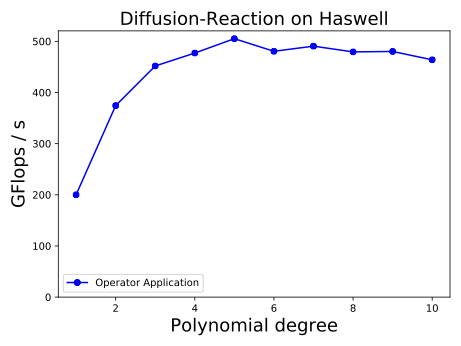 style="width:49.0%" />
 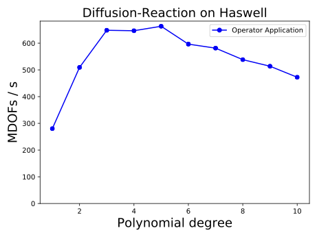 style="width:49.0%" />
Figure 14 shows node level performance numbers for a Discontinuous Galerkin finite element operator for the diffusion reaction equation on an Intel Haswell node. The measurements use MPI to saturate the node and make extensive use of SIMD instructions which lead to a performance of roughly 40% of the theoretical peak performance of 1.17 TFlops/s ($`10^{12}`$ floating point operations per second) on this 32 core node. Discontinuous Galerkin discretizations benefit best from this compute-bound algorithm, as they allow to minimize memory transfers by omitting the costly setup of element-local data structured, operating directly on suitably blocked global data structures instead. A dedicated assembler for DG operators, , is now available in . It does not gather/scatter data from global memory into element-local data structures, but just uses views onto the global data. By this it avoids unnecessary copy operations and index calculations. This assembler is essential to achieve the presented node level performance, but can also be beneficial for traditional DG implementations.
It is worth noting that iterative solvers based on this kind of matrix-free operator evaluation require the design of preconditioners that preserve the low memory bandwidth requirements while ensuring good convergence behavior, as the per-iteration speedup would otherwise be lost to a much higher number of solver iterations. We studied matrix-free preconditioning techniques for Discontinuous Galerkin problems in . This matrix-free solution technology have been used for an advanced application with the Navier–Stokes equations in .
Multiscale methods
There has been a tremendous development of numerical multiscale methods in the last two decades including the multiscale finite element method (MsFEM) , the heterogeneous multiscale method (HMM) , the variational multiscale method (VMM) or the local orthogonal decomposition (LOD) . More recently, extensions to parameterized multiscale problems have been presented, such as the localized multiscale reduced basis method (LRBMS) or the generalized multiscale finite element method (GMsFEM) . In we have demonstrated that most of these methods can be cast into a general abstract framework that may then be used for the design of a common implementation framework for multiscale methods, which has been realized in the module . In the following, we concentrate on an efficient parallelized implementation of MsFEM within the DUNE software framework.
Multiscale model problem
As a model problem we consider heterogeneous diffusion. Given a domain $`\Omega \subset \mathbb{R}^n`$, $`n \in \mathbb{N}_{>0}`$ with a polygonal boundary, an elliptic diffusion tensor $`A^{\epsilon} \in \left(L^{\infty}(\Omega)\right)^{n \times n}`$ with microscopic features, and an $`f \in L^2(\Omega)`$ we define our model problem as
\begin{align}
\label{eq:ms:original-problem} \mbox{find} \quad u^{\epsilon} \in \mathring{H}^1(\Omega):
    \quad \int_{\Omega} A^{\epsilon} \nabla u^{\epsilon} \cdot \nabla \Phi
        = \int_{\Omega} f \Phi \quad \forall \Phi \in \mathring{H}^1(\Omega)
\end{align}with $`\mathring{H}^1(\Omega) \colonequals \overline{\mathring{C}^{\infty}(\Omega)}^{\|\cdot\|_{H^1(\Omega)}}`$.
For the discretization of Equation ([eq:ms:original-problem]) we require a regular partition $`\ensuremath{\mathcal{T}}_H`$ of $`\Omega`$ with elements $`T`$ and a nested refinement $`\ensuremath{\mathcal{T}}_h`$ of $`\ensuremath{\mathcal{T}}_H`$ with elements $`t`$ and choose associated piece-wise linear finite element spaces $`U_H \colonequals S^1_0(\ensuremath{\mathcal{T}}_H) \subset U_{h} \colonequals S^1_0(\ensuremath{\mathcal{T}}_h)\subset \mathring{H}^{1}(\Omega)`$.
We assume that $`U_h`$ is sufficiently accurate. By $`A^{\epsilon}_h`$ we denote a suitable piecewise polynomial approximation of $`A^{\epsilon}`$, and for $`T \in \ensuremath{\mathcal{T}}_H`$, we call $`U(T)`$ an admissible environment of $`T`$, if it is connected, if $`T \subset U(T) \subset \Omega`$ and if it is the union of elements of $`\ensuremath{\mathcal{T}}_h`$. Admissible environments will be used for oversampling. In particular $`T`$ is an admissible environment of itself.
The MsFEM in Petrov–Galerkin formulation with oversampling is defined in the following. The typical construction of an explicit multiscale finite element basis is already indirectly incorporated in the method. Also note that for $`U(T) = T`$ we obtain the MsFEM without oversampling.
Let now $`\mathcal{U}_H = \{ U(T)| \enspace T \in \ensuremath{\mathcal{T}}_H\}`$ denote a set of admissible environments of elements of $`\ensuremath{\mathcal{T}}_H`$. We call $`{\mathcal{R}}^{\epsilon}_h(u_H) \in U_h \subset \mathring{H}^1(\Omega)`$ the MsFEM-approximation of $`u^{\epsilon}`$, if $`u_H \in U_H`$ solves:
\begin{align*}
 \sum_{T \in \ensuremath{\mathcal{T}}_H} \int_{T} A^{\epsilon}_h \nabla {\mathcal{R}}^{\epsilon}_h(u_H) \cdot \nabla \Phi_H = \int_{\Omega} f \Phi_H
      \quad \forall \Phi_H \in U_{H}.
\end{align*}For $`\Phi_H \in U_{H}`$, the reconstruction $`{\mathcal{R}}^{\epsilon}_h(\Phi_H)`$ is defined by $`{\mathcal{R}}^{\epsilon}_h(\Phi_H)_{|T}\colonequals \tilde{Q}_{h}^{\epsilon}(\Phi_H) + \Phi_H`$, where $`\tilde{Q}_{h}^{\epsilon}(\Phi_H)`$ is obtained in the following way: First we solve for $`Q_{h,T}^{\epsilon}(\Phi_H) \in \mathring{U}_h(U(T))`$ with
\begin{align}
 \label{eq:msfem:local} \int_{U(T)} A^{\epsilon}_h \left( \nabla \Phi_H + \nabla Q_{h,T}^{\epsilon}(\Phi_H) \right) \cdot \nabla \phi_h = 0
      \quad \forall \phi_h \in \mathring{U}_h(U(T))
\end{align}for all $`T \in \ensuremath{\mathcal{T}}_H`$, where $`\mathring{U}_h(U(T))`$ is the underlying fine scale finite element space on $`U(T)`$ with zero boundary values on $`\partial U(T)`$. Since we are interested in a globally continuous approximation, i.e. $`{\mathcal{R}}^{\epsilon}_h(u_H) \in U_h \subset \mathring{H}^1(\Omega)`$, we still need a conforming projection $`P_{H,h}`$ which maps the discontinuous parts $`Q_{h,T}^{\epsilon}(\Phi_H)_{|T}`$ to an element of $`U_h`$. Therefore, if
\begin{align*}
 P_{H,h} : \{ \phi_h \in L^2(\Omega)| \enspace \phi_h \in U_h(T) \enspace \forall T \in \ensuremath{\mathcal{T}}_H\} \longrightarrow U_h
\end{align*}denotes such a projection, we define
\begin{align*}
\tilde{Q}_{h}^{\epsilon}(\Phi_H) \colonequals P_{H,h}( \sum_{T \in \ensuremath{\mathcal{T}}_H} \chi_T Q_{h,T}^{\epsilon}(\Phi_H))
\end{align*}with indicator function $`\chi_T`$.
For a more detailed discussion and analysis of this method we refer to .
Implementation and parallelization
Our implementation of the general framework for multiscale methods (, ) is an effort birthed from the project and is built using the Generic Discretization Toolbox (, ) and as well as the core modules described in Section 5.
To maximize CPU utilization we employ multi-threading to dynamically load balance work items inside one CPU without expensive memory transfer or cross-node communication. This effectively reduces the communication/overlap region of the coarse grid in a scenario with a fixed number of available cores. Within we decided to use Intel’s Thread Building Blocks (TBB) library as our multithreading abstraction.
Let us now consider an abstract compute cluster that is comprised of a set of processors $`\mathcal{P}`$, where a set of cores $`C_{P_i} = \{C^j_{P_i}\}`$ is associated with each $`P_i\in \mathcal{P}`$ and a collection of threads $`t_{C_j} = \{t^k_{C_j}\}`$. For simplicity, we assume here that $`j=k`$ across $`\mathcal{P}`$.
Since we are interested in globally continuous solutions in $`U_H`$, we require an overlapping distribution $`\mathcal{T}_{H,P_i} \subset \mathcal{T}_{H}`$ where cells can be present on multiple $`P_i`$. Furthermore, we denote by $`\mathcal{I}_i \subset \mathcal{T}_{H,P_i}`$ the set of inner elements, if for all $`T_H \in \mathcal{I}_i \Rightarrow T_H \notin \mathcal{I}_j`$ for all $`i,j`$ with $`i\neq j`$. The first important step in the multiscale algorithm is to solve the cell corrector problems ([eq:msfem:local]) for all $`U(T_H), T_H \in \mathcal{I}_i`$. These are truly locally solvable in the sense of data independence with respect to neighbouring coarse cells. We build upon extensions to the module made within , presented in , that allow us to partition a given into connected ranges of cells. The assembler was modified to use TBB such that different threads iterate over different of these partitions in parallel (Fig. 15).
For each $`T_H`$ we create a new structured to cover $`U(T_H)`$. Next we need to obtain $`Q_{h,T}^{\epsilon}(\Phi_H)`$ for all $`J`$ coarse scale basis function. After discretization this actually means assembling only one linear system matrix and $`J`$ different right hand sides. The assembly handled by , which is parametrized by an elliptic operator and corresponding right hand side functionals . The performs loop-fusion by merging cell-local operations of any number of input functors. This allows to perform the complete assembly in one single sweep over the grid, using a configurable amount of thread-parallelism.
Since the cell problems usually only contain up to about 100,000
elements it is especially efficient to factorize the assembled system
matrix once and then backsolve for all right hand sides. For this we
employ the UMFPACK direct solver from the SuiteSparse library 9 and
its abstraction through . Another layer of abstraction on top of that in
allows us to switch to an iterative solver at run-time, should we exceed
the suitability constraints of the direct solver.
After applying the projections $`P_{H,h}`$ to get $`\tilde{Q}_{h}^{\epsilon}(\Phi_H)`$, we discretize Eq. ([eq:msfem:local]) which yields a linear system in the standard way. Since this is a system with degrees of freedom (DoF) distributed across all $`P_i`$ we need to select an appropriate iterative solver. Here we use the implementation of the bi–conjugate gradient stabilized method (BiCGSTAB) in , preconditioned by an Algebraic Multigrid (AMG) solver, see Section 5.2. We note that the application of the linear solver for the coarse system is the only step in our algorithm that requires global communication. This allows the overall algorithm to scale with high parallel efficiency in setups with few coarse grid cells per rank, where a distributed iterative solver cannot be expected to scale with its runtime dominated by communication overhead. We demonstrate this case in Figure 16.
While the module can function as a standalone application to apply the method to a given problem, it is also possible to use it as a library in other modules as well (see for example ). Run-time parameters like the problem to solve, oversampling size, micro and macro grid resolution, number of threads per process, etc. are read from a structured INI-style file or passed as a object. New problems with associated data functions and computational domains can easily be added by defining them in a new header file. The central library routine to apply the method to a given problem, with nulled solution and prepared grid setup is very concise as it follows the mathematical abstractions discussed above.
void Elliptic_MsFEM_Solver::apply( DMP::ProblemContainer& problem, const CommonTraits::SpaceType& coarse_space, std::unique_ptr<LocalsolutionProxy>& solution, LocalGridList& localgrid_list) const CommonTraits::DiscreteFunctionType coarse_msfem_solution(coarse_space, “Coarse Part MsFEM Solution”); LocalProblemSolver(problem, coarse_space, localgrid_list).solve_for_all_cells(); CoarseScaleOperator elliptic_msfem_op(problem, coarse_space, localgrid_list); elliptic_msfem_op.apply_inverse(coarse_msfem_solution); //! projection and summation identify_fine_scale_part(problem, localgrid_list, coarse_msfem_solution, coarse_space, solution); solution->add(coarse_msfem_solution);
📊 논문 시각자료 (Figures)
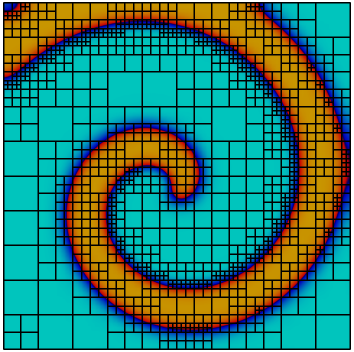
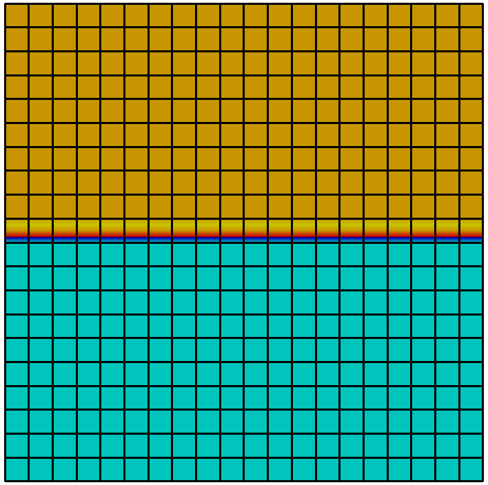
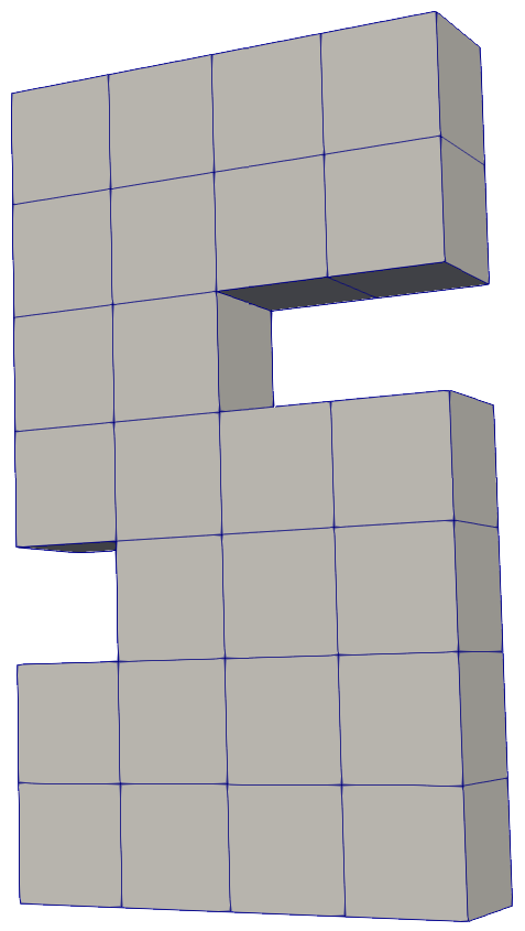
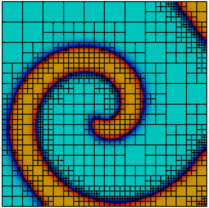
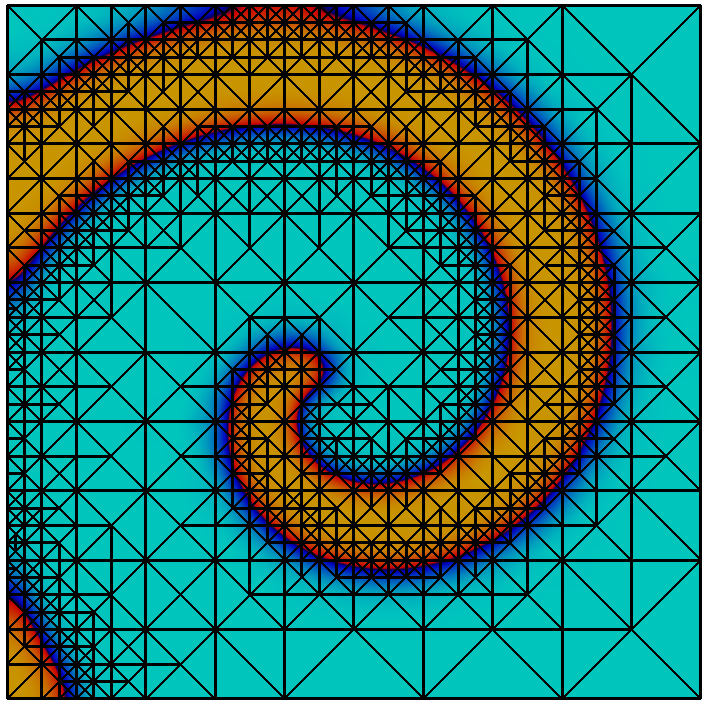
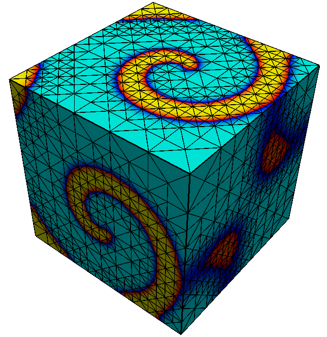
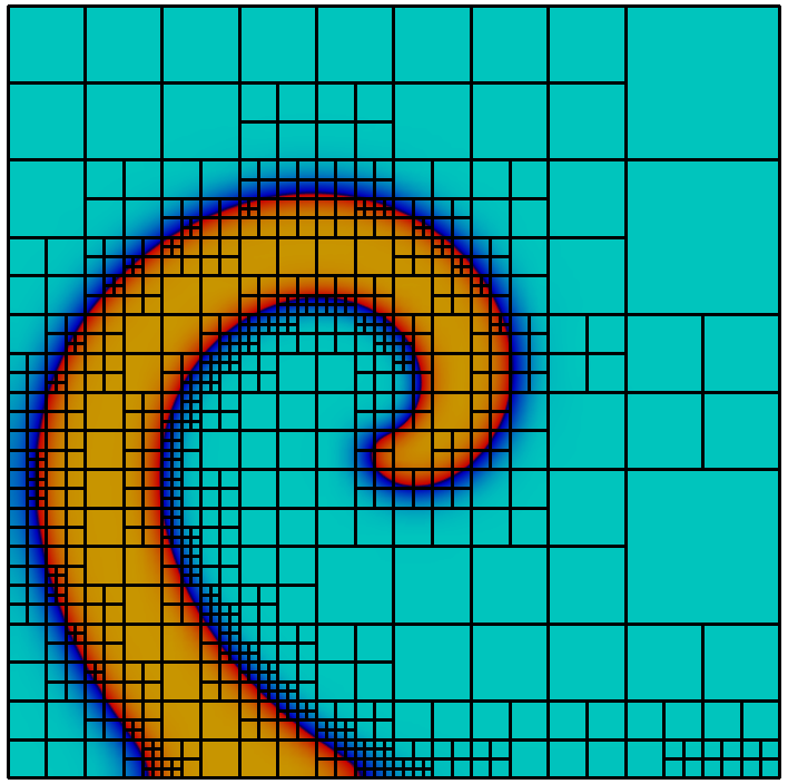
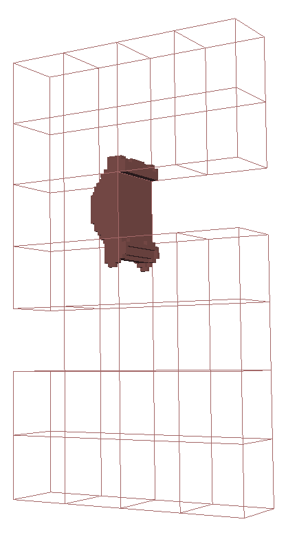
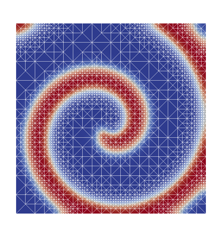
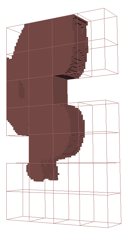
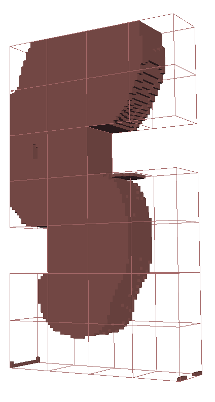
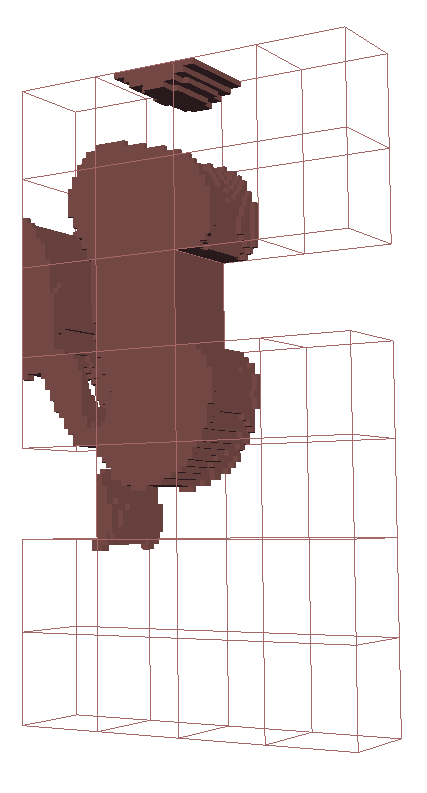
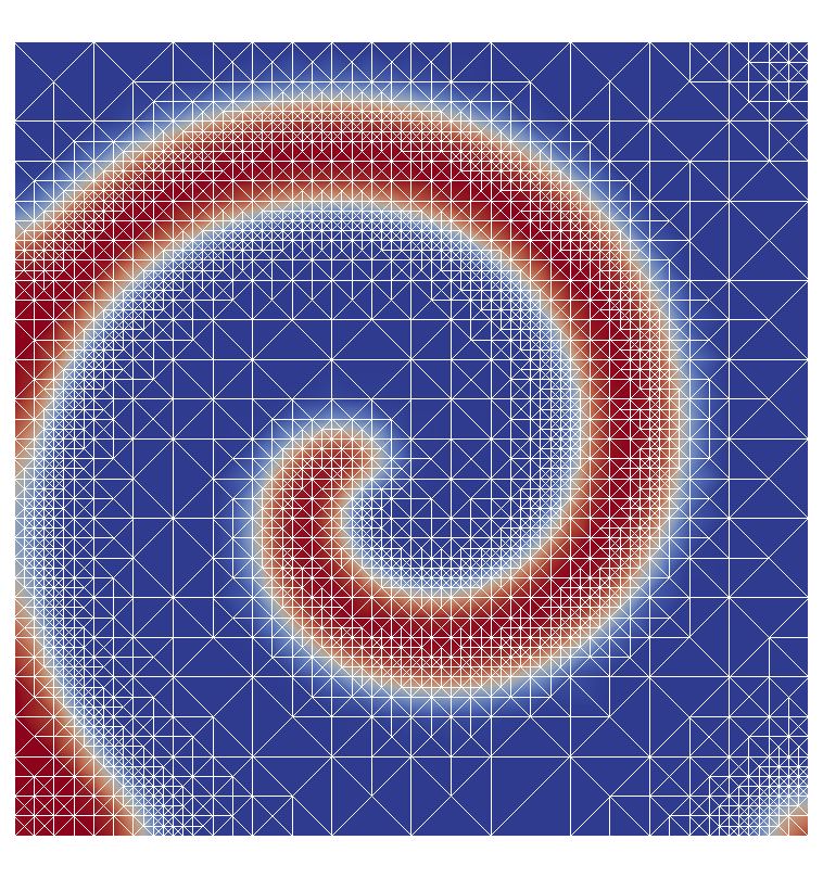
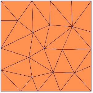
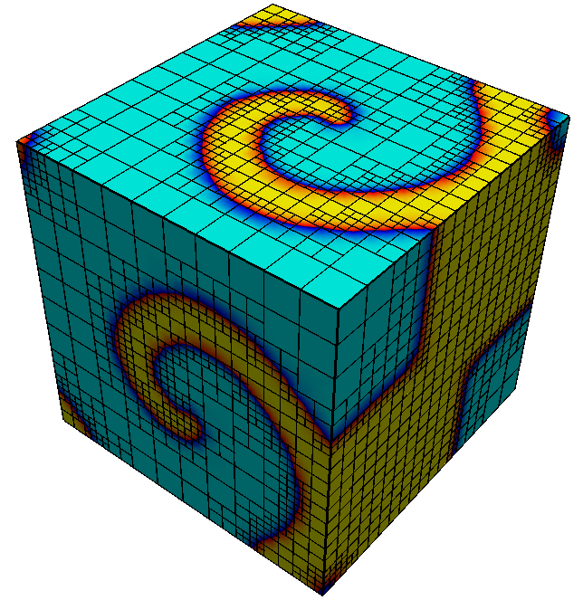
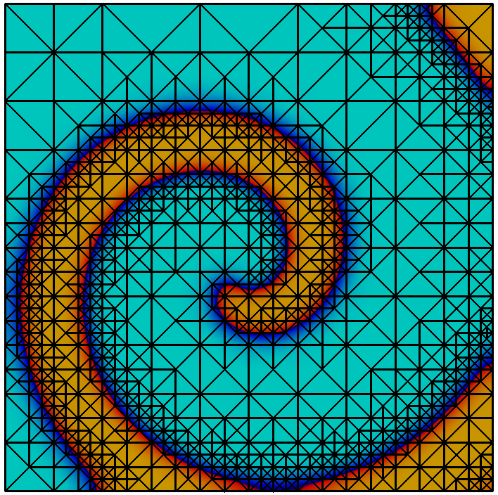
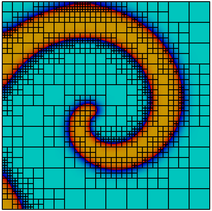
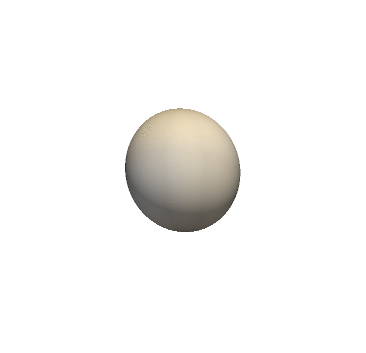
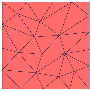

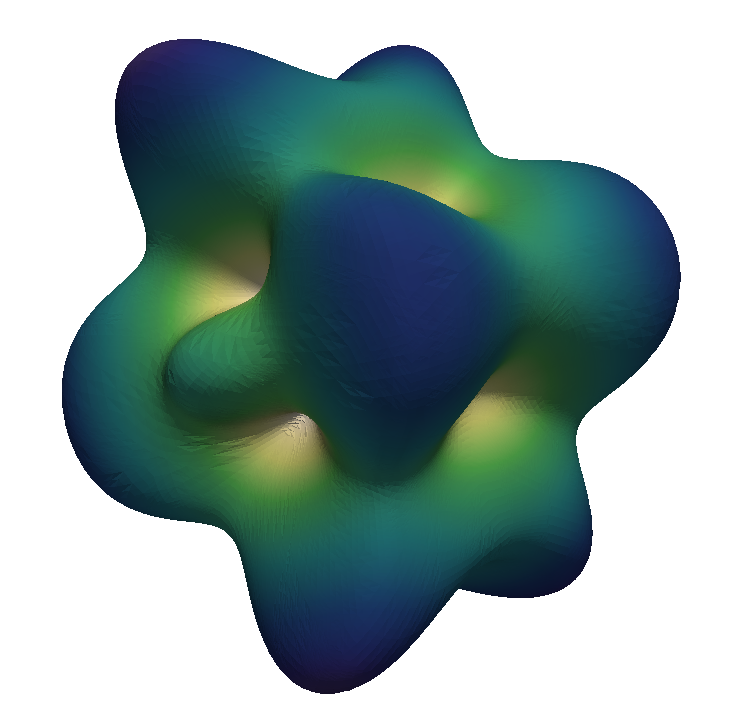
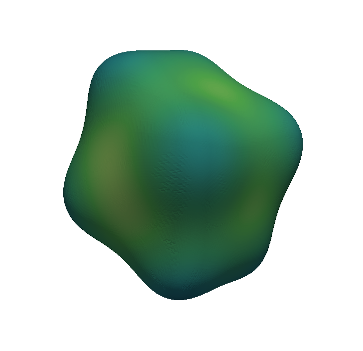
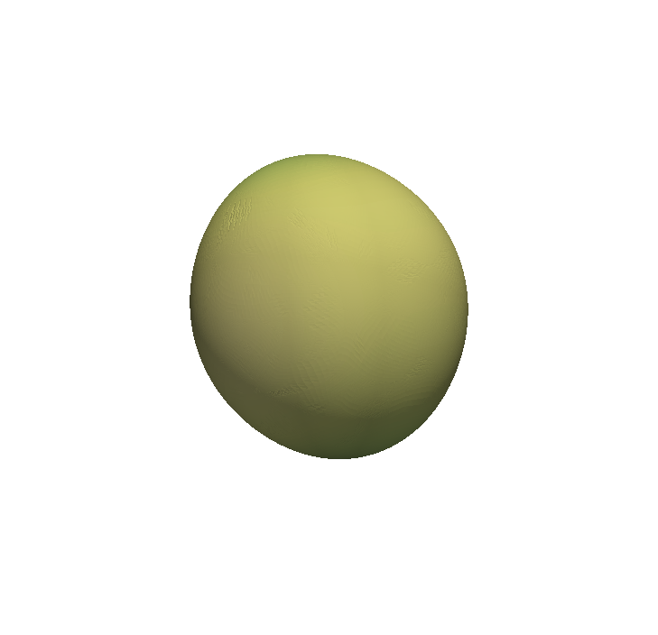
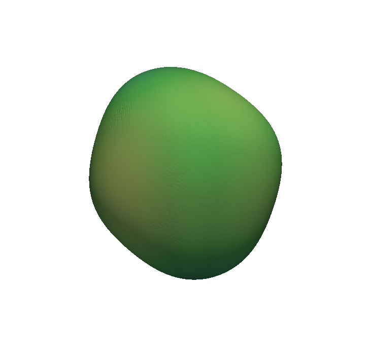
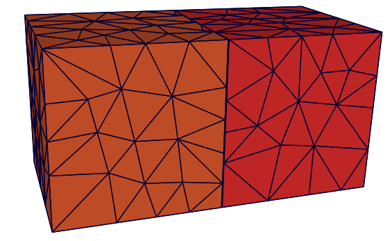
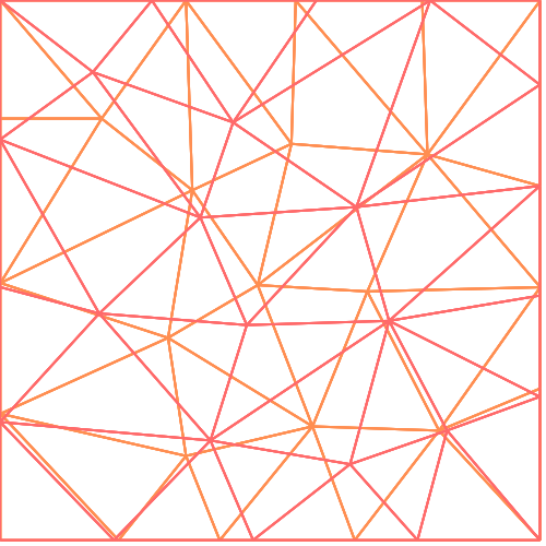
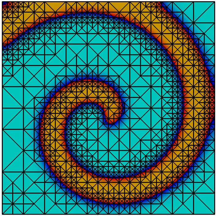
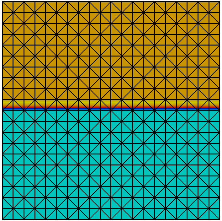
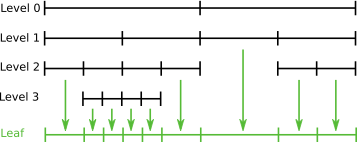
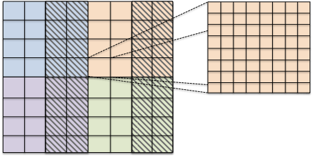
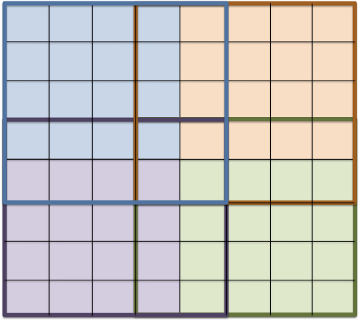
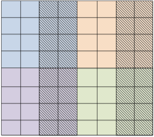
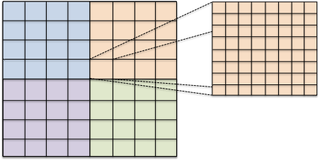
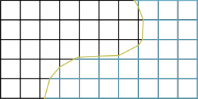
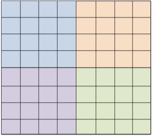
A Note of Gratitude
The copyright of this content belongs to the respective researchers. We deeply appreciate their hard work and contribution to the advancement of human civilization.-
It is called because it can also handle the case where the two subdomains are separated by a physical gap, which is common in contact problems. ↩︎
-
The only exception to this are the multigrid transfer operators. These require access to finite element bases, but are not central to TNNMG. ↩︎
-
See http://math.boisestate.edu/~calhoun/www_personal/research/amr_software/ . ↩︎
-
Used characteristics rather than actual type for algorithms: “if it walks like a duck and quacks like a duck, it is a duck” ↩︎
-
standard template library ↩︎
-
note that an interface similar to Vc is part of the C++ Parallelism TS 2 standard ↩︎