No Delay Latency-Driven and Application Performance-Aware Cluster Scheduling
📝 Original Paper Info
- Title: No Delay Latency-Driven, Application Performance-Aware, Cluster Scheduling- ArXiv ID: 1903.07114
- Date: 2019-08-20
- Authors: Diana Andreea Popescu and Andrew W. Moore
📝 Abstract
Given the network latency variability observed in data centers, applications' performance is also determined by their placement within the data centre. We present NoMora, a cluster scheduling architecture whose core is represented by a latency-driven, application performance-aware, cluster scheduling policy. The policy places the tasks of an application taking into account the expected performance based on the measured network latency between pairs of hosts in the data center. Furthermore, if a tenant's application experiences increased network latency, and thus lower application performance, their application may be migrated to a better placement. Preliminary results show that our policy improves the overall average application performance by up to 13.4% and by up to 42% if preemption is enabled, and improves the task placement latency by a factor of 1.79x and the median algorithm runtime by 1.16x compared to a random policy on the Google cluster workload. This demonstrates that application performance can be improved by exploiting the relationship between network latency and application performance, and the current network conditions in a data center, while preserving the demands of low-latency cluster scheduling.💡 Summary & Analysis
This paper addresses the challenge of optimizing application performance in data centers by considering network latency. The core idea is to develop a scheduling policy, NoMora, that places applications based on their expected performance given the measured network latencies between hosts within the data center. This approach leverages the relationship between network latency and application performance, aiming to improve overall performance.The key innovation of NoMora lies in its ability to model and predict how changes in network latency affect application performance. By continuously measuring these latencies and adjusting the placement of applications accordingly, it can significantly enhance the efficiency and speed at which tasks are executed within a cluster environment.
The results show that NoMora improves overall average application performance by up to 13.4% and by up to 42% if preemption is enabled. Additionally, it reduces task placement latency by a factor of 1.79x and the median algorithm runtime by 1.16x compared to a random policy on Google’s cluster workload.
This work is significant because it provides a practical framework for cloud operators to optimize resource allocation in real-time based on dynamic network conditions. The approach can be particularly beneficial in environments where network latency plays a critical role in application performance, leading to more efficient and responsive data center operations.
📄 Full Paper Content (ArXiv Source)
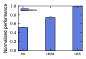
We run an experiment with a Memcached server running in one VM, and four clients running on five different VMs in one cloud provider (Microsoft Azure). The clients send requests to the server using the Mutilate benchmark for a period of time, and we measure the number of requests per second reported by the benchmark. We perform this experiment ten times using the same setup (same specifications for hosts and the same software), but in three different settings. The VMs were deployed in the Korea South zone (KS), then in the UK South zone on a Sunday evening, when there the network is less utilized ), and again in the UK South zone during the day on Monday after restarting the VMs. Figure 1 shows the performance obtained in the three cases normalised with respect to the maximum obtained performance (in UK South during Sunday evening). The performance obtained differs between the three different scenarios, and even within the same zone, with less than 80% of the performance achieved in the second scenario, and with only 50% performance achieved in the first scenario. There is a performance difference depending on the placement of the application and the current network conditions in the . In this situation, knowing how the application reacts to network conditions would guide the placement within the . If the application is already running and the network conditions change, reducing the application’s performance, then it can be migrated to a different placement.
 style="width:98.0%" />
 style="width:98.0%" />
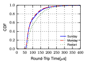
In a different experiment, we observed that network latency is not constant between VMs, as can be seen from Figure 2 during an experiment run during the week of 27th of January 2019. In this experiment we measured the Round-Trip Time (RTT) overal several hours (10 million measurements) using UDP probes between two basic type VMs rented from a different cloud provider (GCP). The first two experiments use the same VMs during different periods of time, and as can be seen the results are similar. For the third run, we restarted the VMs, and got different latencies than in the previous two cases.
 />
/>
Predicting application performance
Obtaining experimental data
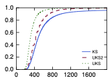
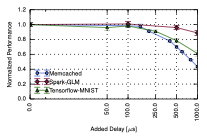
To determine the relationship between network latency and application performance, we used a methodology previously described in , where we injected increasing amounts of latency in a networked system using a latency appliance that delays the packets by a fixed amount of time, and we measured how the application performance changes depending on the amount of inserted network latency. The experimental testbed is the one described in . Each host has an Intel Xeon E5-2430L v2 Ivy Bridge CPU with six cores, running at 2.4GHz with 64GB RAM, and is equipped with an Intel X520 NIC with two SFP+ ports, being connected at $`10`$Gbps through an Arista 7050Q switch. The hosts run Ubuntu Server 16.04, kernel version 4.4.0-75-generic. Each application has a certain performance metric (see Table [tab:app-settings]). We first determined a baseline application performance, where the application runs on a number of hosts with optimal performance for the workload and on that specific setup (see Table [tab:app-settings]). After the baseline performance is determined for each application, we introduced a constant latency value between a host (on which the server/the master component of an application runs) and the other hosts (on which the clients/the workers of an application run) in both directions (send and receive), sweeping the range of values between $`1\mu`$s and $`500\mu`$s. Thus, the total latency values introduced range between $`2\mu`$s and $`1000\mu`$s. We chose values in this range based on the network latency values that we measured in different cloud providers in a previous work . The application performance was measured for each injected latency value, and the experiments were run for each value a sufficient number of times to ensure reproducibility. The experimental results can be seen in Figure 3 in the ’Actual’ line. The complete results are presented in the technical report . This fixed amount of latency represents an amount of latency that can have different causes, such as physical distance, or the delay introduced by the network apparatus, , NICs, switches. However, increased network utilisation can lead to higher latency even if two hosts are close to each other.
| Application | Host’s role | #Hosts | Performance | Runtime | Workload/ | Dataset |
| Metric | Target | Dataset | Size | |||
| Memcached | Server | 5 | Queries/sec | 10 seconds | FB ETC | see |
| STRADS | Coordinator | 6 | Training time | 100K iterations | Lasso Regression | 10K samples, 100K features |
| Spark | Master | 8 | Training time | 100 iterations | GLM Regression | 100K samples, 10K features |
| Tensorflow | Master | 9 | Training time | 20K iterations | MNIST | 60K examples |
Modeling performance
We now construct a function that predicts application performance
dependent upon network latency for each application. To model the
relationship between network latency and application performance, we use
SciPy’s curve_fit function, which uses non-linear least squares to
fit a function p, to the experimental data. The curve_fit returns
optimal values for the parameters, so that the sum of the squared error
of $`\mathit{p}(x\_data, parameters) - y\_data`$ is minimised. The
function has one independent variable, the static latency, and the
dependent variable is the application’s performance metric. We
additionally use the standard deviation of the results as a parameter
for the curve_fit function. We first normalise the values of the
application performance with respect to the baseline performance. We
then model the relationship between network latency and normalised
application performance by fitting a polynomial function to the results,
where the independent variable is the static latency, and the dependent
variable is the normalised performance:
\begin{equation}
Normalised\_performance = \mathit{p}(static\_latency)
\end{equation}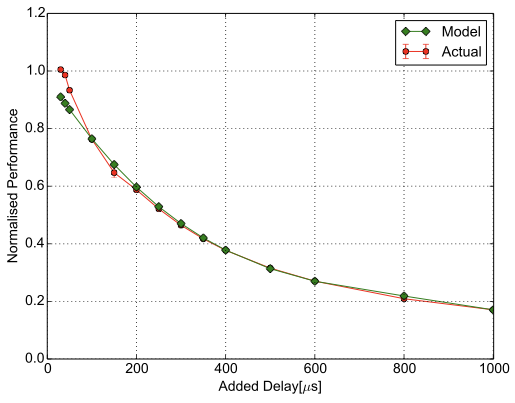 style="width:95.0%" />
 style="width:95.0%" />
 style="width:95.0%" />
 style="width:95.0%" />
Key-value store: Memcached
Memcached is a widely used, in-memory, key-value store for arbitrary data. Clients can access the data stored in a memcached server remotely over the network. We use the Mutilate Memcached load generator, with the Facebook “ETC” workload, taken from , which is considered representative of general-purpose key-value stores. We consider Memcached’s application performance metric the number of queries per second (QPS). The resulting model is shown in Figure [fig:model-2d-memcached] and in Equation [eq:memcached]. This model does not capture the baseline performance, nor small static latency values. Therefore, the model needs to have two functions: a constant function, whose value is the baseline performance, and a logarithmic function fit on the experimental data. The first function gives the performance up to the threshold latency value beyond which the application performance starts to drop, , $`40`$. The Figure [fig:model-2d-memcached] does not show the first function.
\begin{equation}
\label{eq:memcached}
\small
p(x) = \begin{cases}
        1, x < 40 \\
        1.067 - 3.093 \times 10^{-3} \times x + 4.084 \times 10^{-6} \times x^2 - \\ \; \; \; \; - 1.898 \times 10^{-9} \times x^3, x \geq 40
        \end{cases}
\end{equation}Machine Learning applications
STRADS Lasso Regression
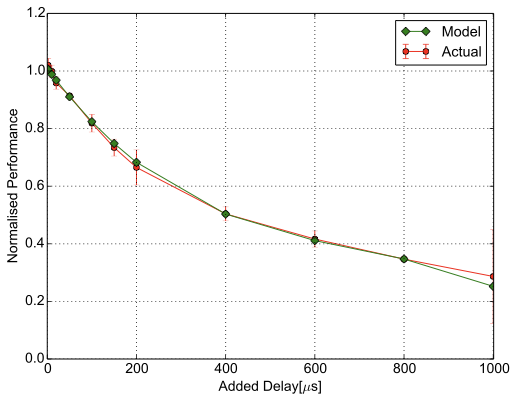
STRADS is a distributed framework for machine learning algorithms targeted to moderate cluster sizes between 1 and 100 machines. We evaluate the impact of network latency on the Lasso Regression application implemented in this framework. The network communication pattern can be represented as a star, with a central coordinator and scheduler on the master server, while workers communicate only with this master server. Since we do not allow the use of stale parameters during iterations (no pipelining) and the injected network latency does not change the scheduling of the parameters, the application performance metric can be represented by the job completion time, named in the next sections the training time. The results are shown in Figure [fig:model-2d-strads] and in Equation [eq:strads]. The first function is the constant baseline performance up to $`20`$.
\begin{equation}
\label{eq:strads}
\small
p(x) = \begin{cases}
        1, x < 20\\
        1.009 - 2.095 \times 10^{-3} \times x + 2.571 \times 10^{-6} \times x^2 - \\ \; \; \; \; - 1.232 \times 10^{-9} \times x^3, x \geq 20
        \end{cases}
\end{equation}Spark GLM Regression
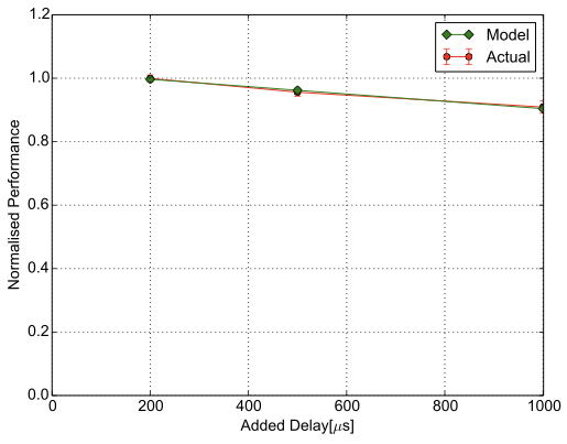
We use Apache Spark ’s machine learning library (MLlib), on top of which we run the GLM regression benchmark from Spark-Perf . We run Spark 1.6.3 in standalone mode. Spark follows a master-worker model. Spark supports broadcast and shuffle, which means that the workers do not communicate only with the master, but also between themselves, but even so, small latencies injected between every pair of hosts do not affect its performance. We use as application performance metric the training time, , the time taken to train a model. The results are shown in Figure [fig:model-2d-spark] and in Equation [eq:spark]. The first function is the constant baseline performance up to $`200`$.
\begin{equation}
\label{eq:spark}
\small
p(x) = \begin{cases}
        1, x < 200\\
        -1.161 \times 10^{-4} \times x + 1.0199, x \geq 200
        \end{cases}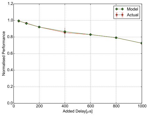
\end{equation}Tensorflow Handwritten Digits Recognition
Tensorflow is a widely used machine learning framework. We use the
MNIST dataset for the handwriting recognition task as input data, and
Softmax Regression for the training of the model. Tensorflow follows a
master-worker model. The application performance metric used is
the training time, similarly to Spark’s performance metric. We use the
synchronise replicas option, which means that the parameter updates
from workers are aggregated before being applied in order to avoid stale
gradients. The results are shown in
Figure [fig:model-2d-tensorflow]
and in Equation [eq:tensorflow]. The first function
is the constant baseline performance up to $`40`$.
\begin{equation}
\label{eq:tensorflow}
\small
p(x) = \begin{cases}
        1, x < 40\\
        1.005 - 5.146 \times 10^{-4} \times x + 5.837 \times 10^{-7} \times x^2 -  \\ \; \; \; \; - 3.46 \times 10^{-10} \times x^3
        , x \geq 40
        \end{cases}
\end{equation}Model generality
Finding a general relationship between an application’s performance and network latency is not easy. We sought to limit the influence of other factors (OS impact on application, number of cores, number of machines in the setup) on the measured application performance, leaving only the effect of network latency on the application performance.
 style="width:50.0%" />
While the impact of latency on performance evaluated in Section 10.1 was conducted on a specific setup, the results offer an intuition on the application behaviour that can be generalised to other setups and scenarios as well. Even though there are differences between computing platforms, the results have the same scale and follow the same trends. We exemplify this statement by evaluating three of the selected applications (Memcached, Spark GLM Regression and Tensorflow MNIST) on a different setup in a in Microsoft Azure. The setup has one server/master VM and five clients/workers VMs. The VM type is Standard E16s v3 with 16 virtual CPUs and 128 GB memory. We insert latencies of over $`100`$with NetEm at every host. The general trend in Figure 4 is the same as in Figure 3 for the selected applications. In the case of Spark GLM Regression and Tensorflow MNIST, the drop in performance on this setup is steeper than on the local testbed. On the other hand, the Memcached server is less affected on this setup compared with the local testbed. These differences can be the result of any or all of the following factors: virtualisation, different number of hosts, host specifications, different network topology, varying network utilisation due to the shared network in the cloud, latency injection through software emulation instead of through a hardware-based solution.
By fitting a naive model to the experimental datasets determined in this section, we took a first step towards building a more general model. A system that benchmarks the application performance under different configurations and network conditions would help in building a complete application performance profile. Such a system would be used to predict the application performance under different circumstances. The predictions can then be used to inform cloud operators and users in order to find the optimal placement under given network conditions.
Related work
In general, incorporating network demands within the cluster scheduler has been treated as a separate problem from cluster schedulers that take into account only the host resources required by a job.
Network bandwidth guarantees Network throughput variability in cloud providers was an important issue, with bandwidth varying by a factor of five in some cases , leading to uncertain application performance and, consequently, tenant cost. Nowadays, cloud providers’ commercial offerings list the expected network bandwidth for each type of VM. These changes fit with the observation that network bandwidth guarantees have improved in recent years .
This improvement in network bandwidth guaranatees for tenants is the result of substantial research in the area. Allocating network bandwidth between endpoints was first described in the context of Virtual Private Networks (VPN) . In the cloud computing model, the VPN customers can be assimilated with the tenants from the cloud, and a VPN endpoint’s equivalent is a VM. The customer-pipe model is the allocation of bandwidth on paths between source-destination pairs of endpoints of the VPN. In this model, a full mesh between customers is required to satisfy the SLAs. In the hose model, an endpoint is connected with a set of endpoints, but the bandwidth allocation is not specified between pairs. Instead, the aggregate bandwidth required for the outgoing traffic to the other endpoints and the aggregate bandwidth required for the incoming traffic from the other endpoints in the hose is specified. These two models served as basis for bandwidth allocation in the cloud, with the hose model being frequently used . SecondNet introduces an abstraction called virtual data centre (VDC) and multiple types of services. Gatekeeper and EyeQ use the hose model and set minimum bandwidth guarantees for sending and receving traffic for a VM, which can be increased up to a maximum rate if unused capacity is available. ElasticSwitch provides minimum bandwidth guarantees by dividing the hose model guarantees into VM-to-VM guarantees, and taking the minimum between the guarantees of the two VMs. Oktopus uses the hose model (virtual cluster, where all the VMs are connected through a single switch) and virtual oversubscribed cluster model (groups of virtual clusters connected through a switch with an oversubscription factor). Proteus authors analyse the traffic patterns of several MapReduce jobs, finding that the network demands of the applications change over time. They propose a time-varying network bandwidth allocation scheme, which is a variant of the hose model. CloudMirror derives a network abstraction model, tenant application graph, based on the application’s communication pattern, which have multiple tiers or components, and bandwidth within the component is allocated using the hose model. Profiling applications to determine their network throughput can help allocate bandwidth in a more efficient manner . This is similar to modeling the relationship between application performance and network latency based on experimental data, as we have done in Section 10. Choreo measures the network throughput between VM pairs through packet trains, estimates the cross traffic, and locates bottleneck links. Based on the network measurements and application profiles (number of bytes sent), it makes VM placement decisions to minimise application completion time. The Choreo system is the closest system to the NoMora cluster scheduling architecture, where we use network latency measurements between pairs of hosts and application performance predictions dependent upon current network latency to decide where to place tenants’ VMs. VM placement when providing network bandwidth guarantees usually starts by looking at subtrees in the topology to place the VMs, and goes upward in the tree to find a suitable allocation . CloudMirror additionally incorporates an anti-colocation constraint in the VM placement algorithm to ensure availability. SecondNet builds a bipartite graph whose nodes are the VMs on the left side and the physical machines on the right side, and then finds a matching based on the weights of the edges of the graph using min-cost max-flow. The weights are assigned based on the available bandwidth of the corresponding server. This approach is similar to Quincy and Firmament , which also model the scheduling problem as a min-cost max-flow problem. Firmament’s network-aware policy avoids bandwidth oversubscription at the end-host by incorporating applications network bandwidth demands into the flow graph. proposes an algorithm for traffic-aware VM placement that takes into account the traffic rates between VMs, and studies how different traffic patterns and network architectures impact the algorithm’s outcome.
Tail network latency guarantees Silo controls tenant’s bandwidth to bound network queueing delay through packet pacing at the end-host. It then places VMs using a first-fit algorithm, while trying to place a tenant’s VMs to minimise the amount of network traffic that the core links have to cary. QJump computes rate limits for classes of applications, ranging from latency-sensitive applications for which it offeres strict latency guarantees to throughput-intensive ones for which latency can be variable. SNC-Meister provides latency guarantees for lower percentiles, , $`99.9`$percentile, admitting more tenants in a as a result. It analyses tenant traces and computes their tail latencies, and then performs VM admission control.
Background on cluster scheduling
 style="width:80.0%" />
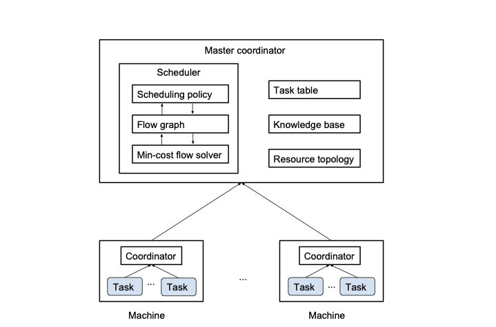
NoMora extends the Firmament cluster scheduler . We chose to extend Firmament because it is a centralised scheduler that considers the entire workload across the whole cluster, making it straightforward to incorporate the network latency measured between every pair of hosts in the cluster, and due to its low latency (sub-second) task placement . Firmament exposes an API to implement scheduling policies, that may incorporate different task constraints. A scheduling policy defines a flow network representing the cluster, where the nodes define tasks and resources. The policy can also use task profiles to guide the task placement through preference arcs to machines that meet the criteria desired by the task. Events such as task arrival, task completion, machine addition to the cluster, or machine removal from the cluster, change the flow network. When cluster events change the flow network, Firmament’s min-cost flow solver computes the optimal flow on the updated flow network. The updates to the flow network caused by the cluster events are not applied while the solver runs, but only after the solver finishes computing the optimal solution. After the solver finishes running, Firmament extracts the task placements from the optimal flow, and applies these changes in the cluster. We next give an overview of how the cluster scheduling problem is mapped to the minimum-cost maximum-flow optimisation problem, as described in Quincy and Firmament .
Flow network Firstly, we provide a high-level overview of the structure of the flow network, which can be seen in Figure 5. By flow network we refer to a directed graph where each arc has a capacity and a cost to send flow across that arc. Each submitted task $`T_{i,j}`$, representing task $`j`$ of job $`J_{i}`$, is represented by a vertex in the graph, and it generates one unit of flow. The sink $`S`$ drains the flow generated by the submitted tasks. A task vertex needs to send a unit of flow along a path composed of directed arcs in the graph to the sink $`S`$. The path can pass through a vertex that corresponds to a machine (host) $`M_{m}`$, meaning the task is scheduled to run on that machine, or it can pass through a special vertex for the unscheduled tasks of that job $`U_{i}`$, meaning that the task is not scheduled. In this way, even if the task is not scheduled to run, the flow generated by this task is routed through the unscheduled aggregator to the sink.
The graph can have an arc between every task and every machine, but this would make prohibitive the computation of an optimal scheduling solution in a short time, as the graph would scale linearly with the number of machines in the cluster. To reduce the number of arcs in the graph, a cluster aggregator $`X`$ and rack aggregators $`R_{r}`$ have been introduced in Quincy, inspired by the topology of a typical . The cost of the arc between a task and the cluster aggregator is the maximum cost across all of the machines in the cluster. Similarly, the cost of the arc between a task and a rack aggregator $`R_{r}`$ is the maximum cost across all of the machines in that rack. It can be easily seen that the costs to the cluster and rack aggregators serve as a conservative approximation, providing an upper bound for a set of resources that are grouped together.
Capacity assignment Each arc in the flow network has a capacity $`c`$ for flow, bounded by $`c_{min}`$ and $`c_{max}`$. In Firmament and Quincy, $`c_{min}`$ is usually zero, while $`c_{max}`$ depends on the type of vertices connected by the arc and on the cost model. Given that the minimum capacity is zero, it is omitted from here onwards, with only the maximum capacity values being presented. The capacity of an arc between a task and any other vertex is $`1`$. If a machine has $`C`$ cores and a rack has $`m`$ machines, the capacity of an arc between a rack aggregator and a machine is $`C`$, and the capacity of an arc between the cluster aggregator and a rack is $`C\times m=Cm`$. The capacity of an arc between a machine and the sink is $`C`$. The capacity between an unscheduled aggregator $`U_{i}`$ and the sink $`S`$ is represented by the difference between the maximum number of tasks to run concurrently for a job $`J_{i}`$, $`F_{i}`$, and the minimum number of tasks to run concurrently for job $`J_{i}`$, $`E_{i}`$, with $`0 \leq E_{i} \leq F_{i} \leq N_{i}`$, where $`N_{i}`$ is the total number of tasks in job $`J_{i}`$. These limits can be used to ensure a fair allocation of runnable tasks between jobs . In the NoMora policy, this capacity is set to $`1`$.
Cost assignment The cost on an arc represents how much it costs to schedule any task that can send flow on this arc on any machine that is reachable via this arc.
Task to machine arc: The cost on the arc between a task vertex $`T_{i,j}`$ and a machine vertex $`M_{m}`$ is denoted by $`d_{i,j,m}`$, and is computed according to information regarding the task and machine. In most cases, this cost is being decreased by how much the task has already run, $`\beta_{i, j}`$ .
Task to resource aggregator arc: The cost on the arc between a task vertex $`T_{i,j}`$ and a rack aggregator vertex $`R_{r}`$, denoted $`c_{i,j,r}`$, represents the cost to schedule the task on any machine within the rack, and is set to the worst case cost amongst all costs across that rack. The cost on the arc between a task vertex $`T_{i,j}`$ and the cluster aggregator $`X`$, denoted by $`b_{i,j}`$, represents the cost to schedule the task on any machine within the cluster, and is set to the worst case cost amongst all costs across the cluster.
Task to unscheduled aggregator arc: The cost on the arc between a task vertex $`T_{i,j}`$ and the unscheduled aggregator $`U_{i}`$, denoted by $`a_{i,j}`$, is usually larger than any other costs in the flow network. The cost on this arc increases as a function of the task’s wait time, in order to force the task to be scheduled, and it is scaled by a constant wait time factor $`\omega`$, which increases the cost of tasks being unscheduled.
Preemption: If preemption is enabled, the scheduler can preempt a task that it is running on a machine, which means the flow pertaining to that task is routed via the unscheduled aggregator, or migrate the task to a different machine, meaning that the flow is routed via that new machine’s vertex. If preemption is not enabled, then a scheduled task will have in the flow network only the arc to the machine that it is currently running on, with all the other arcs being removed once the task is scheduled.
NoMora evaluation
We evaluate NoMora in simulation, using the same simulator as for Firmament’s evaluation, extended to provide network latency measurements between pairs of hosts, and to update them during the simulation. Secondly, we added application performance predictions dependent upon network latency per job and per task (same function for all tasks of a job). Finally, we implemented the policy that uses these predictions and the latency measurements to compute task placements.
Cluster workloads No information about the network communication patterns between a job’s tasks, nor about their sensitivity to network latency are provided in public cluster workloads. Thus, we have assigned the network latency to application performance functions determined in Section 10 to the jobs in the Google workload . We did not include the single task jobs, as they do not communicate with any other task. We used 24 hours of the trace.
Application performance predictions dependent upon network latency The predictions are discretised in steps of 10, and are stored in a hash table for each job. The network latency value between two machines is rounded to the nearest latency value for which the prediction function has an entry in the hash table. For the latency values in the used traces that are outside the interval of defined values, we use the smallest performance value defined for that function. The different prediction functions are assigned randomly in different proportions to the jobs. For the experiments presented in this section, $`50`$% of the jobs use the Memcached prediction, $`25`$% of the jobs use the STRADS prediction and $`25`$% the Tensorflow prediction. This scenario is one of the most challenging, as Memcached is the most latency sensitive application that we studied. we did not use the Spark prediction, which is almost constant, as it would not be challenging to place such jobs. Given the functions built in Section 10, for which the normalised performance does not drop below 0.1, we set $`\gamma=1001`$ for the simulation.
Network latency measurements The simulator leverages the network latency measurements dataset from . With $`18`$ week-long traces provided, we further divide each trace in $`7`$ (for each day of the week), and we assign them to machine pairs considering the physical distance between servers as a criterion. Assuming a typical fat-tree topology for a and based on the latency values measured in Azure by , we use the traces with the lowest values for machine pairs located in the same rack ($`6`$ traces - GCE), the traces with intermediate values for machine pairs located within the same pod ($`6`$ traces - Azure), and the traces with the largest values for machines located in different pods ($`6`$ traces - EC2). These traces are used to provide the latency values between hosts for the duration of the simulation, which is one day. Since we do not have different traces for each machine pair, we scale the values of each trace using a coefficient between 0.8 and 1.2, selected randomly for intra-pod and inter-pod values. For the traces within the rack, we scale them between 0.5 and 1. For the latency values between cores on the same server we use a small constant. Latency values from traces are provided every second in the simulation, in total $`86,400`$ per day between every pair of hosts in the cluster.
Topology We use the Google workload of 12,500 machines . The machines used in the workload are grouped into racks and pods at the beginning and during the simulation. We set the number of machines per rack to 48, and the number of racks per pod to 16. The results will be influenced by the number of hosts per rack and the number of racks per pod due to the assignment of the different cloud latency traces. These two numbers were chosen to reproduce a small cluster. However, if there are more hosts per rack and more racks per pod, then there will be a greater chance to fit all the tasks of a job in the same rack or in the same pod, meaning the job will have a good overall application performance.
We performed experiments with the settings of the Facebook topology (192 hosts per rack and 48 racks per pod) , but for a cluster of only 12,500 machines as the one presented in the Google trace, it means there is only one complete pod and an incomplete one, with a total of approximately 260 racks. The overall application performance in this case is very high due to the small network latencies assigned between the hosts within the same rack.
Evaluation metrics Through the evaluation of the NoMora cluster scheduling policy, we seek to answer the following questions:
-
does NoMora’s placement improve application performance compared to a random placement policy and a load-spreading policy?
-
how long does it take to compute a placement solution?
-
how long does a task have to wait before it runs?
In order to know if our policy improves application performance compared to other policies, we compute the average application performance. This metric measures NoMora’s task placement quality. It is computed as the application performance determined by the network latency in every measurement interval divided by the maximum application performance that could be achieved in every measurement interval, and it is computed for the job’s total runtime.
The algorithm runtime is the time it takes for Firmament’s min-cost max-flow algorithm to run. We compare our policy’s runtime with other Firmament policies’ runtimes to ensure that our policy is scalable when run by a centralised cluster scheduler. Additionally, the time it takes to compute the applications’ placements in a round gives an indication of the time interval that is needed between latency measurements. For example, if the algorithm runtime would be in the order of minutes, running latency measurements every few seconds would not be useful, since the measurements accumulated over the scheduler’s runtime would not be used by the scheduler. On the other hand, if the algorithm runtime is in the order of milliseconds, running latency measurements every second or few seconds is useful, the scheduler being able to use the most recent measurement data.
The task placement latency is the time between task submission and task placement. This metric includes the task wait time, which should be as short as possible, but also the time it takes for Firmament to update the flow network, Flowlessly’s runtime and the time to iterate over the placements computed by Flowlessly. In the context of our policy, the metric also captures by how long the tasks are delayed when they are waiting for their root task to be placed first before them. Another metric that we looked at is the task response time, which is the time between a task’s submission and its completion.
Placement quality
We compare the NoMora policy, using different parameter values for the cost model ([sec:cost-model-params]), with a random policy that uses fixed costs (tasks always schedule if resources are idle), and a load-spreading policy that balances the tasks across machines. We enable preemption only for the NoMora policy, since the two other policies would not benefit from preemption due to their different scheduling goals. The random policy schedules tasks if resources are available, thus migrating a task does not make sense, since the task is already running. The load-spreading policy schedules tasks based on current task counts on machines, thus potential task load imbalance can be handled by scheduling new tasks on less loaded machines instead of migrating already running tasks on the less loaded machines.
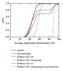
The results for the average application performance for different policies can be seen in Figure 6. we compute the area marked by the $`y`$-axis, the CDF, and the straight horizontal line with $`y=1`$, for each policy. According to this computation, the maximum area corresponding to the maximum average application performance across applications is 100%, and it would be obtained for a vertical line at $`x=100\%`$. Next, we subtract from the NoMora policies areas the random and load-spreading areas to assess the placement improvement given by the NoMora policy. The total area for the random policy is 47.2%, while for the load-spreading policy it is 46.8%. For the NoMora policy with parameters $`p_{m}=105`$ and $`p_{r}=110`$ the area is 60.2%, NoMora with parameters $`p_{m}=105`$ and $`p_{r}=110`$ and preemption enabled is 59%, NoMora with parameters $`p_{m}=110`$ and $`p_{r}=115`$ is 51.85%, and finally, NoMora with parameters $`p_{m}=105`$ and $`p_{r}=110`$, and preemption enabled with $`\beta_{i, j}=0`$, is $`89.6`$%. The maximum overall improvement without preemption enabled is $`13`$% over the random policy and $`13.4`$% over the load-spreading policy, and is obtained for NoMora with parameters $`p_{m}=105`$ and $`p_{r}=110`$. If preemption is enabled and $`\beta_{i, j}=0`$ (the time already executed by a task is not considered in the arc cost computation), the improvement is considerable, $`42.4`$% over the random policy, and $`42.8`$% over the load-spreading one.
The improvement in average application performance is not substantial when preemption is not enabled because of the root task’s random placement, and also because of a smaller number of available places a task can be scheduled because of long-running jobs that are set up at the beginning of the trace. The tasks of the jobs are placed in the best available slots in relation to the root task’s placement. In this way, we constrain the available placements, and the policy searches for placements in relation to a known location rather than trying to find the a placement for all the tasks of a job simultaneously. We further explain the reason behind this design decision and its implications in Section 18.
It can be seen that the CDF of NoMora with preemption enabled has a different shape than the other policies. This is due to task preemption, which can correct the initial placement if it is not good (because of the random placement of the root task), and it can also migrate tasks when their current placement is not good anymore. The improvement provided by the NoMora policies without preemption is evident from Figure 6, but it can also be seen that the CDFs start at approximately the same value ($`27`$%-$`28`$% average application performance), and have an initially similar shape to the random and load-spreading CDFs. On the other hand, for NoMora with preemption enabled, the minimum average application performance is $`44`$% and $`84`$% respectively, which means that the improvement in application performance happens across all jobs due to migration to better placements.
 style="width:40.0%" />
Algorithm runtime
The algorithm runtime depends on the number of arcs from each task to the resources, but also on the cluster size. As the number of arcs or the cluster size increases, so does the algorithm runtime. The two parameters of the cost model ([sec:cost-model-params]) influence the number of arcs the graph has between task nodes and machine nodes or rack nodes, and hence the algorithm runtime, which depends on the flow network size and on the number of tasks considered per scheduling round. If the thresholds are lower, the preference lists will be smaller. In this case, the applications’ performance will be higher (only high-quality placements considered), but they will have less placement options to be scheduled, and thus the wait time may increase. The tasks will have to wait for the machines that offer the performance desired to have empty slots. However, setting a high threshold means the preference lists will be larger, which could lead to an increase in the algorithm runtime. On the other hand, more placement options will be available for the tasks to be scheduled, reducing their wait time. In practice, the algorithm runtime may not necessarily increase. With more placement options available, the tasks may be scheduled sooner, thus leading to less tasks being scheduled per round, resulting in a decrease in the algorithm runtime per scheduling round.
 style="width:40.0%" />
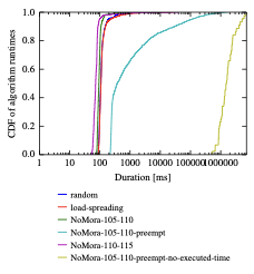
Figure 7 presents results for the algorithm runtime for the load-spreading policy, random policy and for the NoMora policy with and without preemption on the Google workload. The two parameters of the cost model are set as in the previous experiment. The random and load-spreading policies have a similar algorithm runtime, with a median runtime of 108. However, the two policies differ at the tail: for the random policy the 99percentile is 661and a maximum of $`18.89`$s, while for load-spreading policy the 99percentile is 974and a maximum of $`25.88`$s. For NoMora with parameters $`p_{m}=105`$ and $`p_{r}=110`$, the median algorithm runtime is 93(99percentile is 248, and maximum is $`6.13`$s), an improvement of $`1.61\times`$ for the median runtime, and $`2.66\times`$ and $`3.92\times`$ at the 99percentile, compared to the baselines. For NoMora with $`p_{m}=110`$ and $`p_{r}=115`$, median runtime is 72(99percentile is 486, and maximum is $`39.55`$s). On the other hand, the maximum value for the algorithm runtime is considerable larger in the case of NoMora policies.
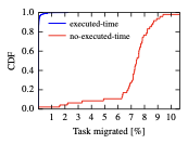
NoMora with parameters $`p_{m}=105`$ and $`p_{r}=110`$ with preemption enabled takes a considerable longer amount of time, because of the higher number of arcs in the flow network compared to the case when preemption is not enabled (the arc preferences of the tasks that are running are not removed, unlike when preemption is not enabled), and the updates made to the flow graph (adding or changing running arcs to resources), further resulting in a larger number of tasks considered per scheduling round. This also translates into a larger task placement latency (13.3). As can be seen from Figure 8, the percentage of migrated tasks in the first case (NoMora with preemption enabled and already executed time for a task considered in the arc computation) is on average $`0.022`$% per scheduling round, with a 99percentile of $`0.5`$%. If $`\beta_{i, j}=0`$ (already executed time is not considered in the arc computation), a considerable number of task migrations take place: an average of $`7.1`$% per scheduling round, with a 99percentile of $`10.07`$%. This happens because the time a task has already run is ignored in the arc cost computation, meaning that the cost is based solely on the expected application performance under the given network conditions. The median algorithm runtime time is 373, the 99percentile is 511s and the maximum is $`1719`$s, which is $`3.45\times`$ larger than the baseline for the median runtime, and $`773\times`$ larger than the baseline at the 99percentile. In the second case ($`\beta_{i, j}=0`$), the median running time is $`1532`$s, the 99percentile $`6610`$s, and the maximum is $`7118`$s. This significant algorithm runtime means that preemption should be used with care. For example, only certain applications that explicitly demand to be migrated should be migrated, or migration can be triggered only if the application performance drops below a certain threshold.
 style="width:40.0%" />
Task placement latency
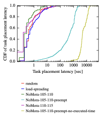 style="width:40.0%" />
Figure 9 presents the task placement latency, which is at the median 436, 90percentile is 312and 99percentile is 1.9s for the random policy; median is 498, 90percentile is 4.3s and 99percentile is 25s for the load-spreading policy, median is 278, 90percentile is 1.23s and 99percentile is 5.8s for the NoMora policy with parameters $`p_{m}=105`$ and $`p_{r}=110`$; median is 185, 90percentile is 1s and 99percentile is 5.6s for the NoMora policy with parameters $`p_{m}=110`$ and $`p_{r}=115`$; median is 519s, 90percentile is 1484s and 99percentile is 2458s for the NoMora policy with preemption enabled and parameters $`p_{m}=105`$ and $`p_{r}=110`$; and median is 4812s, 90percentile is 13077s and 99percentile is 16251s for the NoMora policy with preemption enabled, $`\beta_{i, j}=0`$ and parameters $`p_{m}=105`$ and $`p_{r}=110`$.
The NoMora policy with parameters $`p_{m}=105`$ and $`p_{r}=110`$ improves the median task placement latency by $`1.56\times`$ compared to the random policy and by $`1.79\times`$ compared to the load-spreading policy. The NoMora policy with parameters $`p_{m}=110`$ and $`p_{r}=115`$ improves the median task placement latency by $`2.35\times`$ compared to the random policy and by $`2.69\times`$ compared to the load-spreading policy.
 style="width:40.0%" />
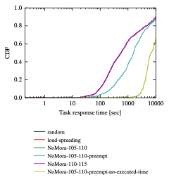
In Figure 10, it can be seen that the NoMora policy with preemption degrades the task response time, because of longer task placement latencies (Figure 9). The CDF is truncated to 10,000s, because the trace includes long-running jobs that span the whole trace.
Conclusion
We introduced latency-driven, application performance-aware cluster scheduling, and NoMora, a cluster scheduling framework that implements this type of policy. It exploits functions that predict application performance based upon network latency and dynamic network latency measurements between hosts to place tasks in a , providing them with improved application performance. The overall application performance improvement given by NoMora depends on the workload, network topology and on the network conditions in the . Using the Google cluster workload augmented with cloud latency measurements from and with performance prediction functions, we showed that the NoMora policy improves the overall average application performance by up to $`13.4`$% and by up to 42% if preemption is enabled, and improves the task placement latency by a factor of $`1.79\times`$ and the median algorithm runtime by $`1.16\times`$ compared to the baselines. This demonstrates that application performance can be improved by exploiting the relationship between network latency and application performance, and the current network conditions in a , while preserving the demands of low-latency cluster scheduling.
In future work, we will evaluate our cluster scheduling architecture on different cluster workloads and on an experimental testbed.
Acknowledgements
We would like to thank Ionel Gog and Malte Schwarzkopf for helping with Firmament. We would like to thank Noa Zilberman, who developed the latency appliance used to conduct the measurements described in Section 10.1, and previously presented in . The latency appliance was first published in , and was open sourced in March 2017 and can be found at .
Given the network latency variability observed in data centers, applications’ performance is also determined by their placement within the data centre. We present NoMora, a cluster scheduling architecture whose core is represented by a latency-driven, application performance-aware, cluster scheduling policy. The policy places the tasks of an application taking into account the expected performance based on the measured network latency between pairs of hosts in the data center. Furthermore, if a tenant’s application experiences increased network latency, and thus lower application performance, their application may be migrated to a better placement. Preliminary results show that our policy improves the overall average application performance by up to 13.4% and by up to 42% if preemption is enabled, and improves the task placement latency by a factor of $`1.79\times`$ and the median algorithm runtime by $`1.16\times`$ compared to a random policy on the Google cluster workload. This demonstrates that application performance can be improved by exploiting the relationship between network latency and application performance, and the current network conditions in a data center, while preserving the demands of low-latency cluster scheduling.
📊 논문 시각자료 (Figures)