- Title: Automatic Support Removal for Additive Manufacturing Post Processing
- ArXiv ID: 1904.12117
- Date: 2019-05-30
- Authors: Saigopal Nelaturi, Morad Behandish, Amir M. Mirzendehdel, Johan de Kleer
📝 Abstract
An additive manufacturing (AM) process often produces a {\it near-net} shape that closely conforms to the intended design to be manufactured. It sometimes contains additional support structure (also called scaffolding), which has to be removed in post-processing. We describe an approach to automatically generate process plans for support removal using a multi-axis machining instrument. The goal is to fracture the contact regions between each support component and the part, and to do it in the most cost-effective order while avoiding collisions with evolving near-net shape, including the remaining support components. A recursive algorithm identifies a maximal collection of support components whose connection regions to the part are accessible as well as the orientations at which they can be removed at a given round. For every such region, the accessible orientations appear as a 'fiber' in the collision-free space of the evolving near-net shape and the tool assembly. To order the removal of accessible supports, the algorithm constructs a search graph whose edges are weighted by the Riemannian distance between the fibers. The least expensive process plan is obtained by solving a traveling salesman problem (TSP) over the search graph. The sequence of configurations obtained by solving TSP is used as the input to a motion planner that finds collision free paths to visit all accessible features. The resulting part without the support structure can then be finished using traditional machining to produce the intended design. The effectiveness of the method is demonstrated through benchmark examples in 3D.
💡 Summary & Analysis
This paper discusses an algorithm for automatically removing support structures in the additive manufacturing (AM) process using multi-axis machining tools. The focus is on identifying and separating contact areas between support components and the main part, while ensuring that there are no collisions with evolving 'near-net' shapes or remaining support components.
The problem addressed here is the manual removal of support structures during post-processing, which can be time-consuming and inconsistent in accuracy. This research employs a recursive algorithm to analyze and identify accessible support components by examining contact regions. Each accessible component is represented as a ‘fiber’ within the collision-free space between tool assemblies and evolving ’near-net’ shapes. A search graph is then generated based on these fibers, allowing for the calculation of the most cost-effective process plan through solving the Traveling Salesman Problem (TSP). The results from TSP serve as input for motion planning.
The key achievement of this paper is an automated method for removing support structures that saves time and effort while ensuring accuracy and consistency. This approach is effective in meeting general conditions regarding shape, connectivity, number, or layout of support components and their dislocation features.
This research is significant because it enables the automation of support structure removal during AM processes, significantly reducing time and labor requirements while maintaining high levels of accuracy and reliability. Consequently, this improves the overall efficiency and dependability of product manufacturing processes.
Support Removal , Additive Manufacturing , Post-Processing ,
Accessibility Analysis , Configuration Space
Results
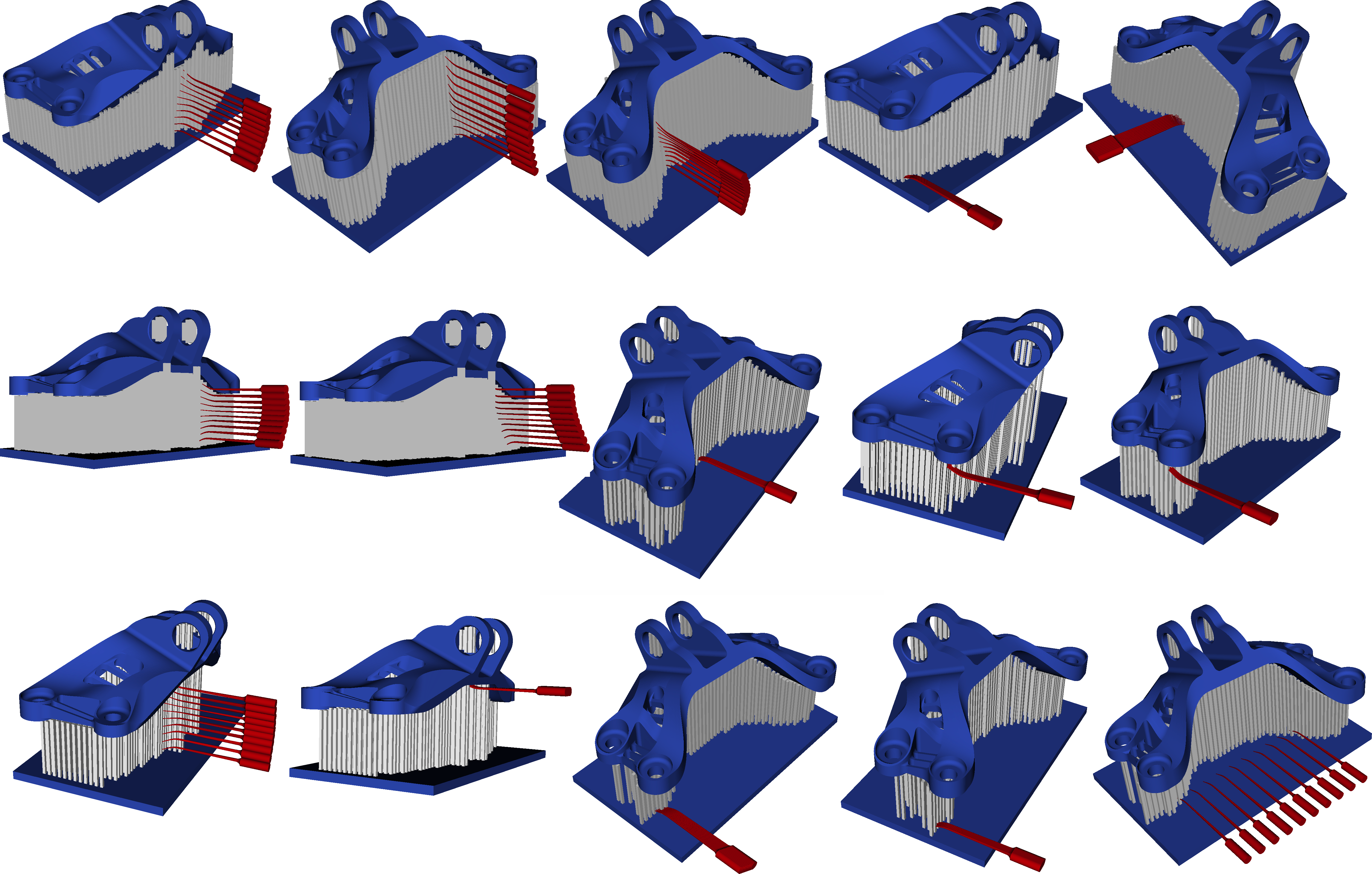
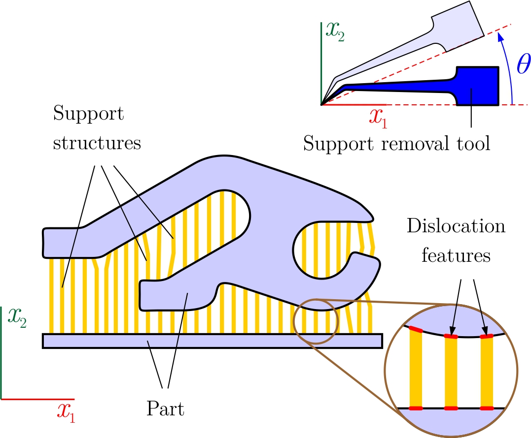
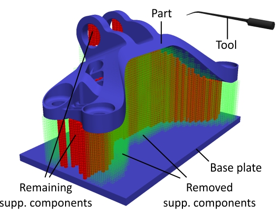
A near-net shape highlighting the AM part (blue), support
removal tool (red), support structure (white), and dislocation features
(green). The support components must be peeled off to fully disengage
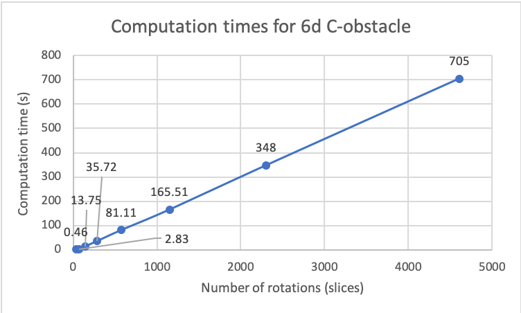
the part without leaving printed material behind.Computation times for the 6DC−space obstacle by sampling rotations and
computing convolutions at a resolution of 5123 to represent each r−slice of the obstacle. The
computations are performed using FFTs via ArrayFire on an NVIDIA GTX 1080 GPU (2,560 CUDA cores, 8GB
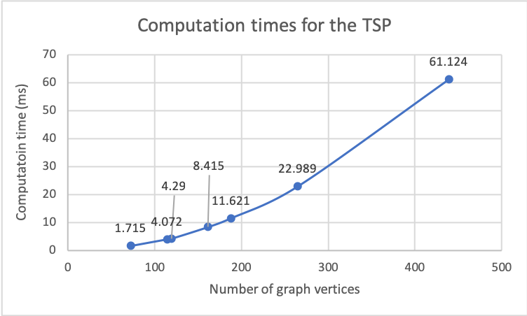
RAM) via OpenCL.Computation times for the TSP in configuration space using
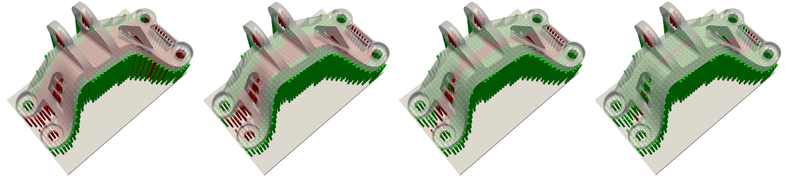
the Boost Graph Library.Several rounds of support removal via Algorithm [alg_recursive]. At each round, a
subset of the support components is connected to the part and the base
plate by dislocation features that are accessible in at least one
orientation.
.
Several intermediate collision-free paths for the cutting
tool to contact the supports at dislocation features. Each row
represents a single recursion of Algorithm [alg_recursive]. Observe that the
motion planner ensures that the tool changes orientation if required
when moving from one dislocation feature to the next. Each individual
collision free path is computed using OMPL in approximately 0.5
seconds
We demonstrate the approach using an illustrative 3D example. A near-net
shape along with a cutting tool to remove supports at dislocation
features is shown in Fig. 1.
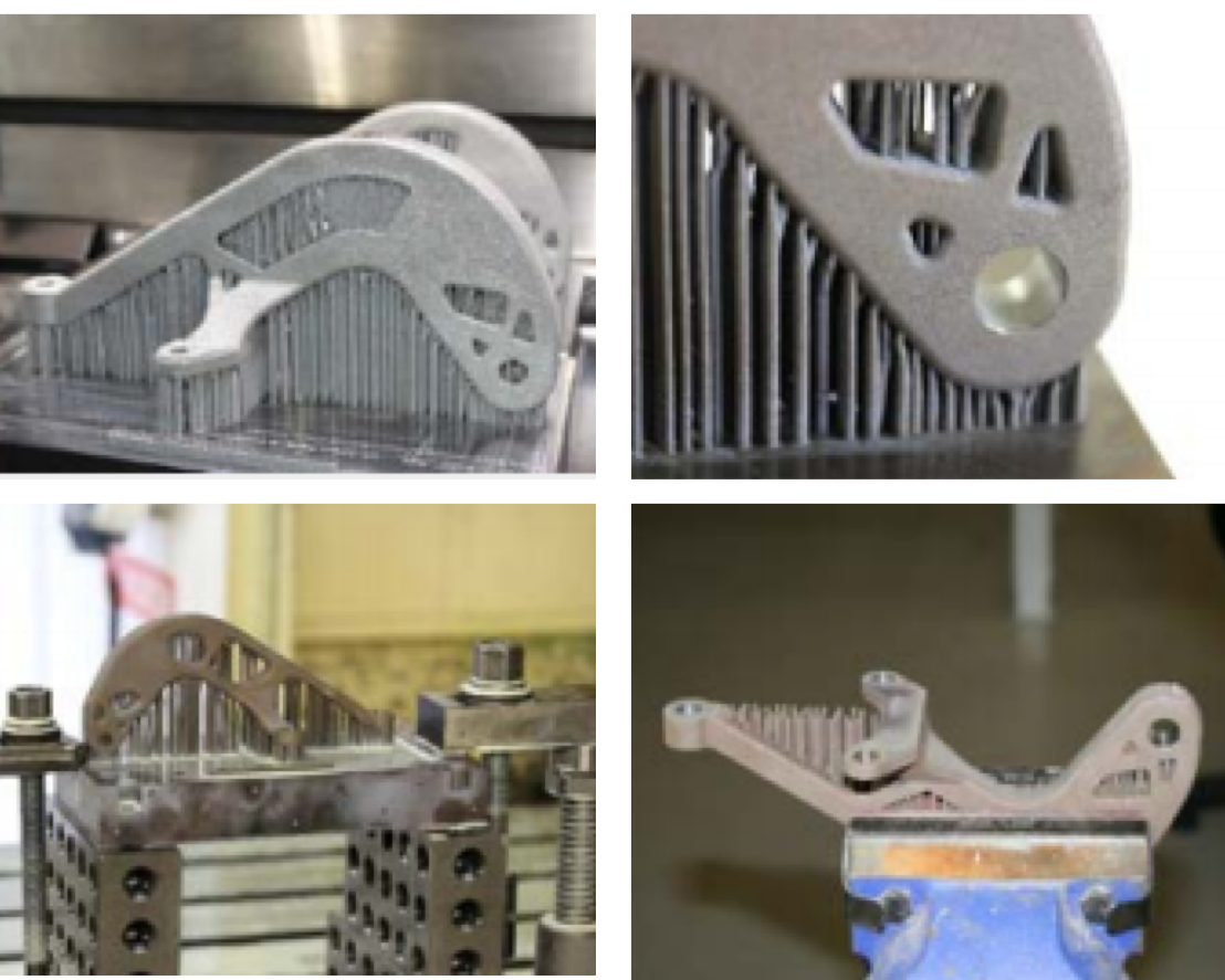
We assume that the part is fixtured properly (not shown here, similarly
to Fig. [fig_metal]) such that the removal
sequence of the support components does not impact its stability.
At every round, Algorithm
[alg_recursive] identifies the outer
layer of supports that can be peeled off, using FFT-based convolution
(Sections 4.1 and
4.2) as illustrated in Fig.
4. For each layer, solving the TSP on
the graph of fibers (Section
5) gives a sequence of configurations to
visit, while asserting all of them will contact a distinct dislocation
feature without collision.
The OMPL motion planner is invoked to
find a collision-free tool-path to fracture the dislocation features one
after another (Section 5.2), as illustrated in Fig.
5.
Figures 2 and
3 show running times for computing
$`{\mathsf{C}}-`$space obstacles and solving TSP, respectively.
Identifying Removable Supports
Removing supports by cutting off their contact regions with the part is
an efficient alternative to machining the entire support material using
a traditional milling process. For the latter, in the same way that one
would remove material from a full raw stock , one can clean out the
support material by sweeping the tool within the support material over
the continuum of accessible configurations. In our approach, we need
only finite contact configurations to peel off the support components.
This assumption is critical in our ability to efficiently compute the
free space for an evolving near-net shape.
At the beginning, it is likely that only a subset of support components
are removable in this manner with a given tool. Intuitively, we may
imagine a forest of support components (e.g., columns) in a near-net
shape, where the occluded columns are inaccessible until the columns
along the periphery are removed.
Our approach uses known properties of the $`{\mathsf{C}}-`$space of
relative rigid transformations (detailed in Sections
4.1 and
4.2) to automatically identify the
maximal collection of supports that are guaranteed to be removable from
a near-net shape in an intermediate state. Briefly, the algorithm
proceeds as follows: The $`{\mathsf{C}}-`$space obstacle is computed
explicitly and all contacting but non-colliding configurations of the
tool are extracted. A support component is deemed removable iff all of
its dislocation features are accessible through contact, meaning that
there exists at least one configuration in the boundary of the
$`{\mathsf{C}}-`$space obstacle that corresponds to each dislocation
feature. All removable support components are collected and designated
for removal at the current “round” of the post-process plan. After
removing this collection from the near-net shape, the
$`{\mathsf{C}}-`$obstacle reduces in size, more dislocation features
become accessible, hence more support components become removable. The
algorithm recursively identifies a sequence of removable supports that
are peeled off by the cutting tool to finally converge to the desired
part.
Note that this process is independent of the precise order and tool-path
1 in which the collected support components of a given round are
removed in practice. A manufacturability test is also encoded in the
algorithm, which can identify early on if the near-net shape includes
support components that are inherently unreachable even after removing
the outer layers.
Constructing Configuration Space Obstacles
We formulate the support removal problem for $`\mathrm{d}-`$dimensional
shapes (typically, $`\mathrm{d}=2`$ or $`3`$). Throughout the paper, we
will use illustrations in 2D for building intuition, and show 3D results
in Section 6.
Queries about the interference of a moving body (e.g., the tool
assembly) $`T
\subseteq {\mathds{R}}^\mathrm{d}`$ against a stationary set of 3D
obstacles (e.g., the near-net shape)
$`N \subseteq {\mathds{R}}^\mathrm{d}`$ are conceptualized as evaluating
membership predicted against the $`{\mathsf{C}}-`$space obstacle
$`\mathcal{O}(N,T) \subseteq {\mathsf{C}}`$ which partitions the
$`{\mathsf{C}}-`$space of relative rigid transformations
$`{\mathsf{C}}:=
{\mathrm{SE}(\mathrm{d})}`$ into three disjoint regions representing
free, contacting, and interfering configurations respectively. These
regions correspond to the exterior, boundary, and interior of the
$`{\mathsf{C}}-`$space obstacle, respectively.
Constructing the obstacle $`\mathcal{O}(N,T)`$ is a critical step in our
algorithm. Practical approaches use the fact that the particular group
structure of $`{\mathrm{SE}(\mathrm{d})}
= {\mathrm{SO}(\mathrm{d})} \rtimes {\mathds{R}}^\mathrm{d}`$ (i.e., the
Lie group of rigid transformations) allows it to be factored into two
simpler and lower-dimensional subgroups; namely,
$`{\mathrm{SO}(\mathrm{d})}`$ (for rotations) and
$`{\mathds{R}}^\mathrm{d}`$ (for translations). Hence, we can represent
each rigid transformation $`\tau \in
{\mathrm{SE}(\mathrm{d})}`$ as a tuple $`\tau \equiv (r, {\mathbf{t}})`$
with $`{\mathbf{t}}\in \mathbb{R}^\mathrm{d}`$ and
$`r \in {\mathrm{SO}(\mathrm{d})}`$. In 2D, the former is a 2D vector
while the latter is represented by a angle $`\theta \in [0, 2\pi)`$. In
3D, the former is a 3D vector while the latter can be represented in a
number of different ways (e.g., orthogonal matrices, quaternions,
axis-angle, Euler angles, etc.).
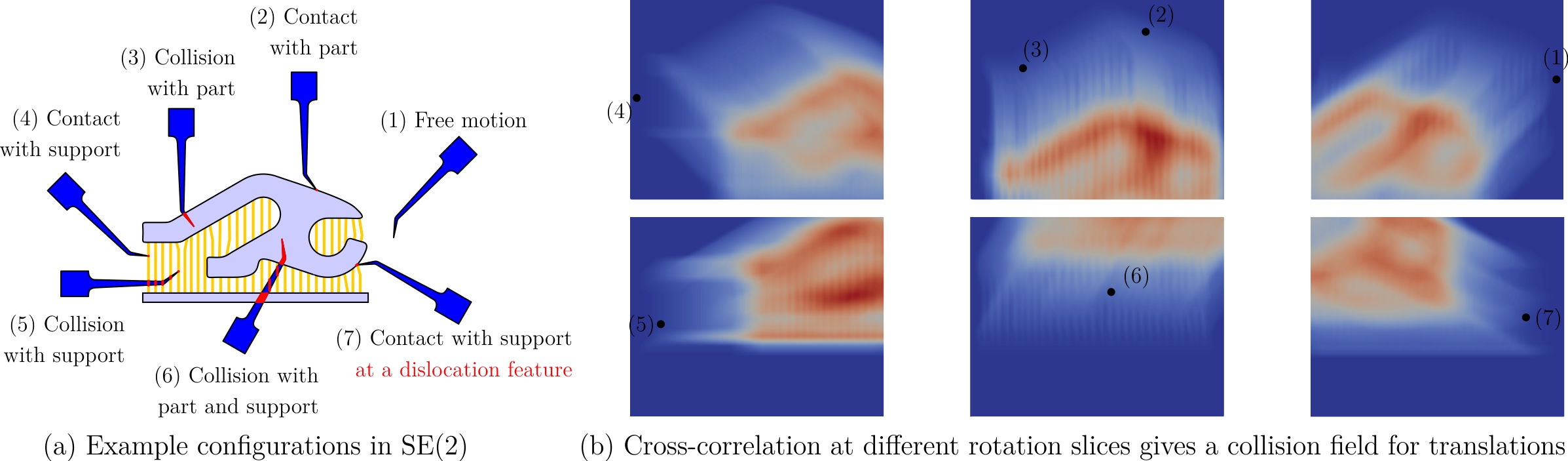
At every iteration of support removal planning, different
tool configuration modes (e.g., free, contact, and collision) are
determined by point membership classification (PMC) against the C−space obstacle. In this 2D example, at
every tool orientation r ∈ SO(2) in (a), the overlap
measure (i.e., area of the interference regions highlighted in red) for
all possible translations is given by a convolution field over the r−slice in (b). For a given
translation (annotated points on the r−slices), the value of the field
determines the overlap measure.
Let us denote a rotation of $`T \subseteq {\mathds{R}}^\mathrm{d}`$ by
$`r \in {\mathrm{SO}(\mathrm{d})}`$ by $`T_r
\subseteq {\mathds{R}}^\mathrm{d}`$. Assuming that we are only dealing
with solids (i.e., compact-regular seminalaytic sets in
$`{\mathds{R}}^\mathrm{d}`$) , the $`{\mathsf{C}}-`$obstacle
$`\mathcal{O}(N,T)`$ may be expressed as follows:
where $`\mathsf{i}(\cdot)`$ represents the topological interior
operator. The pointset $`(N \oplus (-T_r))`$ is the topological closure
of the translational $`{\mathsf{C}}-`$space obstacle of $`N`$ with
$`T_r`$, i.e., the $`{\mathsf{C}}-`$obstacle for a fixed orientation
$`r \in {\mathrm{SO}(\mathrm{d})}`$. It is well-known that this pointset
may be calculated in terms of a Minkowski sum. 2 The
$`{\mathsf{C}}-`$space for all rotations is thus obtained by unifying
the different translational $`{\mathsf{C}}-`$spaces, each forming a
slice of the $`{\mathsf{C}}-`$obstacle. In practice,
$`\mathcal{O}(N,T)`$ may be approximated as a stack of a finite number
of $`r-`$slices, indexed by rotations sampled in
$`{\mathrm{SO}(\mathrm{d})}`$. This approach is commonly used to
calculate $`{\mathsf{C}}-`$space obstacles for planar motions .
Notice that $`(N \oplus (-T_r))`$ represents the closure of the
translational $`{\mathsf{C}}-`$space obstacle and its boundary, denoted
by $`\partial(N \oplus (-T_r))`$ represents all the translations of the
moving body (fir the fixed orientation) that cause surface contact but
no volumetric interference with $`P`$. The contact configurations
$`\mathcal{C}(N,T) \subseteq {\mathrm{SE}(\mathrm{d})}`$ are therefore
obtained as:
The contact space is normally a lower-dimensional submanifold of
$`{\mathrm{SE}(\mathrm{d})}`$, which makes its computation challenging.
In practice, we approximate $`\mathcal{C}(N,T)`$ with a slightly
“thickened” set, i.e., a narrow (but measurable) region surrounding the
boundary of the $`{\mathsf{C}}-`$space obstacle.
Querying Contact Configurations
Our approach uses the fact that the Minkowski sum
$`(A \oplus B) \subseteq
{\mathds{R}}^\mathrm{d}`$ of a pair of arbitrary solids
$`A, B \subseteq {\mathds{R}}^\mathrm{d}`$ corresponds to the support
(i.e., $`0-`$superlevel set) of the convolution $`({\mathbf{1}}_A \ast
{\mathbf{1}}_B)`$ of the indicator functions
$`{\mathbf{1}}_A, {\mathbf{1}}_B: {\mathds{R}}^\mathrm{d}\to \{0,
1\}`$ of the two sets. 3 The advantage of this approach is that the
convolution may be implemented in terms of Fourier transforms. 4 When
the sets are sampled uniformly on a regular grid, the fast Fourier
transform (FFT) provides an efficient and scalable implementation of
each translational $`{\mathsf{C}}-`$space obstacle (i.e, $`r-`$slice of
$`\mathcal{O}(P,T)`$):
A configuration $`\tau \equiv (r, {\mathbf{t}})`$ is inside the obstacle
if the convolution does not vanish for at least one orientation
$`r \in {\mathrm{SO}(\mathrm{d})}`$. Note that the convolution of
nonnegative functions is always nonnegative, hence the free space is
defined implicitly by and equality test:
The convolution provides a field of overlap measure values between
$`P`$ and $`T_r`$ over the translational $`{\mathsf{C}}-`$space. In
other words, $`({\mathbf{1}}_N \ast
{\mathbf{1}}_{-T_r})({\mathbf{t}}) = \mu^\mathrm{d}[N \cap (T_r+{\mathbf{t}})]`$
measures the volume of intersection (if any) between $`P`$ and the moved
body $`T_\tau := (T_r + {\mathbf{t}}) =
\{{\mathbf{x}}+ {\mathbf{t}}~|~ {\mathbf{x}}\in T_r\}`$. Here,
$`\mu^\mathrm{d}[\cdot]`$ represents the Lebesgue $`\mathrm{d}-`$measure
(e.g., area for $`\mathrm{d}= 2`$ and volume for $`\mathrm{d}= 3`$) .
The queried configuration is in the $`{\mathsf{C}}-`$space obstacle
(resp. free space) iff this measure is greater than (resp. equal to)
zero.
The contact space $`\mathcal{C}(P, T)`$ consists of configurations at
which the overlap measure is critically zero, meaning that there
exists an infinitesimal change to the configuration that can make it
nonzero. To approximate $`\mathcal{C}(N,
T)`$ in a computable fashion, we implicitly define an
‘$`\epsilon-`$contact’ space using the following predicate:
Using a small the threshold $`\epsilon > 0`$, one may assume that
$`\mathcal{C}_\epsilon(N, T)`$ closely approximates
$`\mathcal{C}(N, T)`$ from a measure-theoretic standpoint.
To summarize, if the $`r-`$slices are computed and stored beforehand (as
a finite number of convolutions), it is possible to query the overlap
measure in constant time at any sampled translation and rotation by
interpolation against the stack of convolution fields. In particular,
$`\mathcal{C}(N,T)`$ is numerically approximated as the set of all
transformations $`(r,{\mathbf{t}}) \in {\mathrm{SE}(\mathrm{d})}`$ where
$`0 < ({\mathbf{1}}_N \ast
{\mathbf{1}}_{-T_r})({\mathbf{t}}) < \epsilon`$ for some tolerable
interference volume $`\epsilon
0`$.
Figure 6 illustrates in 2D how the
computed stack of convolutions for different $`r-`$slices for sampled
rotations is used to classify a given tool configuration as free,
contact, or colliding. In 3D, the same exact method applies, except that
each convolution is a 3D field and the rotations are samples in 3D using
any number of standard uniform or pseudo-uniform/random sampling methods
.
Algorithm [alg_contact] describes a simple (and
parallel) procedure to compute the $`\epsilon-`$contact space for a
finite sample $`\{r_s\}_{1 \leq s \leq
n_1} \subset {\mathrm{SO}(\mathrm{d})}`$ of orientations. The
convolution is faster to compute on a regular sample
$`\{{\mathbf{t}}_s\}_{1 \leq s \leq n_2} \subset {\mathds{R}}^\mathrm{d}`$
of translations using uniform FFTs , which requires a regular
axis-aligned sample (i.e., voxelization) of the part and rotated tool.
The procedure takes $`O(n_1 n_2 \log n_2)`$ which is very close to
linear time in the number of sampled configurations $`n := n_1 n_2`$.
Note that this procedure is called only once per round of the recursive
outer-loop (Algorithm [alg_removal]). See the results in Fig.
2 of Section
6.
Note that storing the entire 6D set of $`{\mathsf{C}}-`$space obstacle
$`\mathcal{O}(N,T)`$ for 3D parts is not practical. However, the contact
space $`\mathcal{C}(N,T)`$, approximated by
$`\mathcal{C}_\epsilon(N,T)`$, is a sparse subset of the
$`{\mathsf{C}}-`$space that can be precomputed and queried later in
constant-time.
Identifying Removable Support Components
In this Section, we reason about the tool assembly’s free space to
automatically construct a maximal collection of removable support
components. This collection is defined as the set of all support
components that may be removed by the tool assembly without interfering
with the near-net shape, except by the tool tip at the fracture points.
Let $`P, S \subseteq {\mathds{R}}^\mathrm{d}`$ denote the part and
support structure, respectively, which only contact over their common
boundary denoted by $`F := (P
\cap S) = (\partial P \cap \partial S)`$. The initial near-net shape
is obtained as $`N := (P \cup S)`$.
The support structure commonly consists of many connected components
(called hereafter support components):
MATH
\begin{equation}
    S = \bigcup_{1 \leq i \leq n_S} S_i, \quad(S_{i} \cap S_{i'}) = \emptyset
    \quad\text{if}~ i \neq i', \label{eq_components}
\end{equation}
Click to expand and view more
where $`S_i \subseteq {\mathds{R}}^\mathrm{d}`$ stands for the
$`i`$$`^\text{th}`$ component ($`1 \leq i \leq
n_S`$). We assume that a given support component is removable with a
given cutting tool if the tip of the tool can access and fracture all
contact regions between the support component and the part boundary in
one or more collision-free configurations, i.e., positions and
orientations of the tool at which the tool does not interfere with the
part or other support components. The contact region
$`F = (P \cap S) = (\partial P \cap \partial S)`$ is also decomposed
into its connected components (hereafter called dislocation features):
where $`F_j \subseteq {\mathds{R}}^\mathrm{d}`$ stands for the
$`j`$$`^\text{th}`$ feature ($`1 \leq i \leq
n_F`$). Note that the indexing scheme for
([eq_components]) and
([eq_features]) are different because
every support component is connected to the part via two or more
dislocation features hence $`n_F \geq 2 n_S`$. The nomenclature is
illustrated in Fig. 7 for a 2D example.
A 2D near-net shape, including the part and support
structure (i.e., scaffolding), and a support removal tool with three
DOFs (two translations and one rotation). The C−space of rigid motions is SE(2) whose elements are parameterized by
(x1, x2, θ).
Support structures are typically designed to have small contact regions
with the part’s surface to enable easier fracturing and removal and to
minimize surface roughness after removal. Note that sometimes support
components are constructed from one location on the part to another, but
it is preferred that they are constructed connect the part’s surface to
the machine’s base plate. Moreover, one support component can be
connected to the part at multiple locations, e.g., when they are
designed to branch out from a main trunk. To accommodate the most
general condition, we do not make any simplifying assumption on the
shape, connectivity, number, or layout of support components and their
dislocation features.
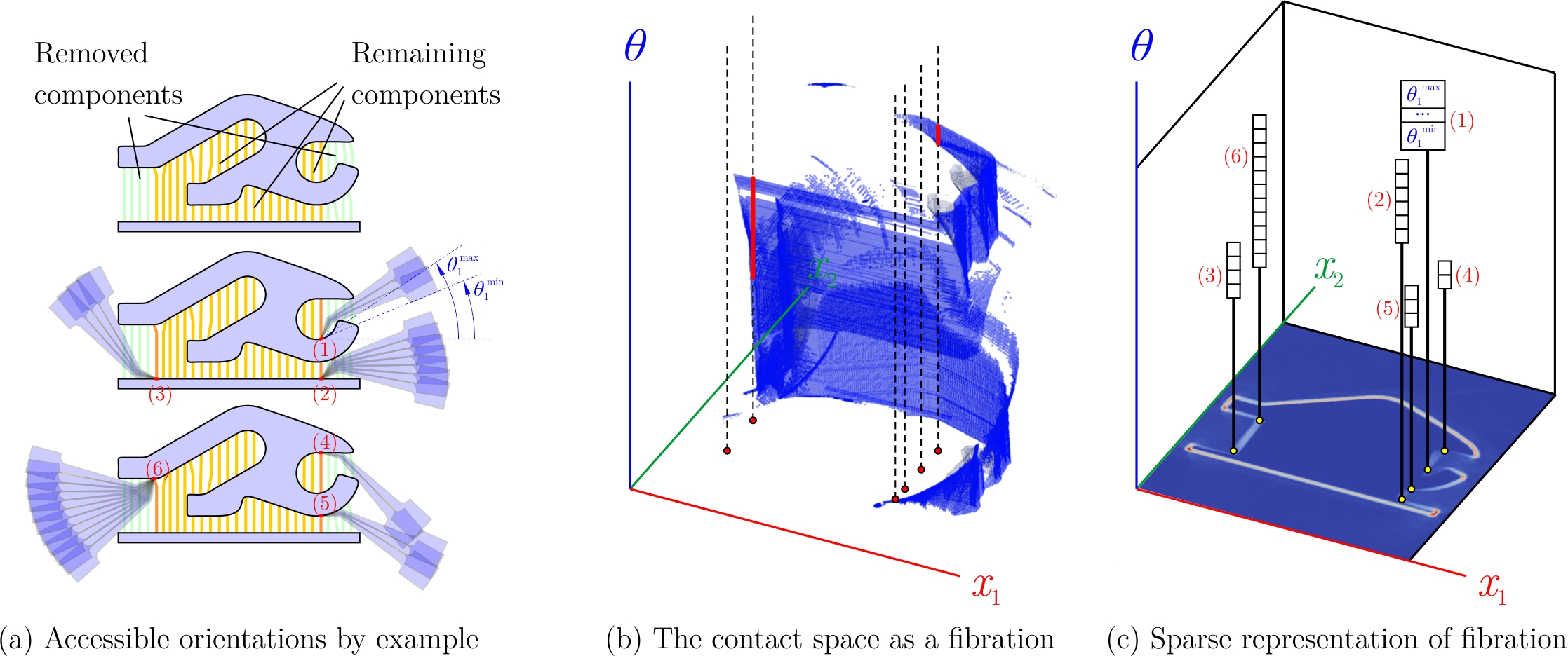
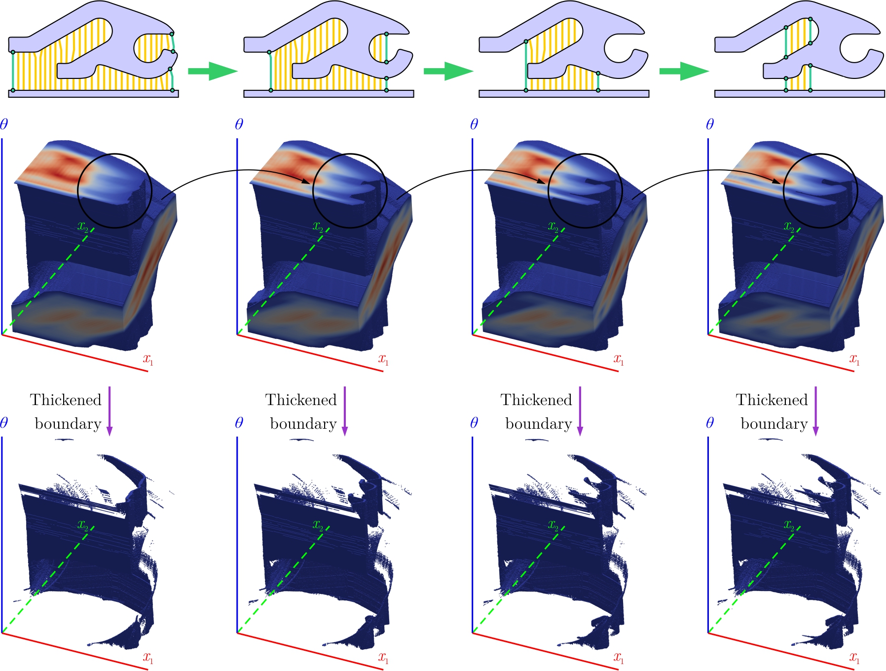
At every recursion of support removal planning, the
accessible dislocation features (exemplified in (a)) are characterized
by their inclusion in the the projection of the contact configurations.
This implies the existence of a nonempty subset of orientations at which
the feature’s lifting by to the C−space
(i.e., a ‘fiber’) intersects the C−space obstacle’s boundary. The resulting
fibration is represented by a list of lists, each containing sampled
orientations at which the dislocation feature is
accessible.
Let us position the tool in its original configuration in such a way
that the cutter tip (or some point on the cutting surface) coincides
with the origin of the coordinate system used as a reference frame to
quantify the rigid transformations of the tool assembly
$`T \subseteq {\mathds{R}}^\mathrm{d}`$ with respect to the near-net
shape $`N \subseteq {\mathds{R}}^\mathrm{d}`$ at a given round. This
choice ensures that a transformation
$`\tau \equiv (r, {\mathbf{t}}) \in {\mathrm{SE}(\mathrm{d})}`$ brings
the tool’s cutter (and not any other point on the tool) to the point
$`{\mathbf{t}}\in {\mathds{R}}^3`$ in the Euclidean $`\mathrm{d}-`$space
where the near-net shape resides. Although this choice is not necessary
from a theoretical standpoint, it simplifies the accessibility analysis
by querying the pre-computed $`{\mathsf{C}}-`$space map.
In a $`\mathrm{d}-`$dimensional space, the tool can operate with all
$`\mathrm{d}(\mathrm{d}+1)/2`$ degrees of freedom,
$`\mathrm{d}(\mathrm{d}-1)/2`$ of which are for rotations and the
remaining $`\mathrm{d}`$ are for translations. We can define
projections from
$`{\mathrm{SE}(\mathrm{d})} = {\mathrm{SO}(\mathrm{d})} \rtimes {\mathds{R}}^\mathrm{d}`$
to $`{\mathrm{SO}(\mathrm{d})}`$ and $`{\mathds{R}}^\mathrm{d}`$,
respectively, that map every rigid transformation
$`\tau \equiv (r, {\mathbf{t}}) \in
{\mathrm{SE}(\mathrm{d})}`$ to $`r \in {\mathrm{SO}(\mathrm{d})}`$ and
$`{\mathbf{t}}\in {\mathds{R}}^\mathrm{d}`$:
Notice that the second projection depends on the earlier choice of
origin. Clearly, these maps are not invertible as functions.
Nonetheless, we can define liftings that take every
$`r \in {\mathrm{SO}(\mathrm{d})}`$ and
$`{\mathbf{t}}\in {\mathds{R}}^\mathrm{d}`$ to a subspace of
$`{\mathrm{SE}(\mathrm{d})}`$: 5
By extension, we can define set functions; for example, $`\pi_2^{-1}:
\mathcal{P}({\mathds{R}}^\mathrm{d}) \to \mathcal{P}({\mathrm{SE}(\mathrm{d})})`$
such that $`\pi_2^{-1}(F)`$ assigns a copy of the entire
$`{\mathrm{SO}(\mathrm{d})}`$ to every point $`{\mathbf{t}}\in F`$:
Given a dislocation feature $`F_j \subset P`$, the set of all
configurations at which it can be touched by the tool tip can be
obtained in terms of the above projection/lifting maps:
In other words, every dislocation feature is lifted to the
$`{\mathsf{C}}-`$space by pairing it with all possible orientations. The
pairing results in the set of all possible configurations that bring the
tool tip to the dislocation feature (at different orientations). Among
them, the ones that are contained within the contact space
$`\mathcal{C}(N, T)`$ are collision-free, hence they represent the set
of all accessible configurations. Hereafter, we refer to
$`\mathpzc{f}_j \subset {\mathrm{SE}(\mathrm{d})}`$ as the contact
fiber for the dislocation feature. Once again, for computational
purposes, we can approximate the contact fibers via $`\epsilon-`$fibers,
using the measurable $`\epsilon-`$contact region:
In practice, the dislocation features are small enough to assume that
touching any point on their circumference is sufficient to fracture
it. As a result, we can simply project the fiber from
$`{\mathrm{SE}(\mathrm{d})}`$ to $`{\mathrm{SO}(\mathrm{d})}`$ to
collect all accessible orientations at all positions within the feature:
Figure 8 illustrates the fibers for a 2D
example in which the dislocation features are contracted to points. From
an algorithmic perspective, each $`\epsilon-`$fiber can be hashed into a
list of sampled orientations anchored at a different dislocation
features. A dislocation feature is accessible iff its fiber is
nonempty. As a result, we observe that a given support component is
removable iff every one of its dislocation features has a nonempty
fiber.
As the near-net shape goes through Algorithm [alg_recursive], the C−space obstacle keeps shrinking in size and
more support structures become removable. At each recursion, the
accessible dislocation features are identified by their fibers, exposed
at the 𝒞ϵ(N, T).
Algorithm [alg_removal] describes the procedure
for finding the contact fibers in a single round of recursive support
removal planning. The procedure performs $`O(n_F)`$ queries on every one
of the convolution fields precomputed and stored for $`n_1`$ sampled
orientations, resulting in a total of $`O(n_F n_1)`$ queries—each
convolution-read taking constant time. This analysis assumes that we
need $`O(1)`$ queries per each dislocation feature, because each feature
is sampled by one or at most a few point(s), which is reasonable. Every
orientation that is accessible is pushed into a stack that represents
the fiber for the queried feature.
Note that before performing the queries, we can shortlist the $`n_F`$
features rapidly to accessible ones by projecting the
$`\epsilon-`$contact space to the Euclidean $`\mathrm{d}-`$space (i.e.,
losing orientation information) and finding its common points with the
dislocation features:
This means that there exists at least one point in the dislocation
feature $`F_j`$ that belongs to the projected contact space. The
projection ensures that there exists at least one non-colliding
orientation at which the said point is accessible. Note that the
projected contact space can be obtained by unifying the translational
contact spaces $`\partial(N \oplus (-T_r))`$ for different orientations:
Once again, the contact space can be approximated by the
$`\epsilon-`$contact criterion. As such, the above early test for
accessibility can be rapidly computed by summing up the indicator
functions of the translational contact spaces, which, in turn, are
obtained as the $`(0, \epsilon)-`$interval level set of the convolution
fields for different $`r-`$slices. The resulting pointset is a single
field over the $`\mathrm{d}-`$space with a narrow support, containing
all positions in the vicinity of the near-net shape’s boundary that can
be accessed by at least one orientation. For every point
$`{\mathbf{t}}\in {\mathds{R}}^\mathrm{d}`$, we accumulate the
convolution value over $`r-`$slices for which the condition
$`0 < ({\mathbf{1}}_N
\ast {\mathbf{1}}_{-T_r})({\mathbf{t}}) < \epsilon`$ holds. This incurs
no additional computation cost because as the convolutions are
precomputed, their $`(0,
\epsilon)-`$interval level sets can be extracted and accumulated
on-the-fly. The result is a field with a narrow-band support over the
$`\mathrm{d}-`$space that quantifies non-colliding orientations of a
given point. A 2D example of the accumulated and projected field of
contact measures is illustrated in Fig.
8 (c) (base field). A dislocation
feature is accessible iff it has at least one point at which this
function is nonzero. Note that this early test counts the accessible
orientations; however, it does not tell us which orientations (i.e.,
the fiber).
Recursive Support Removal Rounds
It is likely that multiple support components are removable from the
near-net shape at a given intermediate state. Intuitively, every round
of the recursive algorithm peels off all removable components to expose
a new set of components. The process is repeated until either all
supports are removed, or the part is deemed non-manufacturable because
some supports are inaccessible. See the results in Fig.
4 of Section
6.
At round$`-\mathtt{t}`$ of the support removal algorithm, 6 the
near-net shape is $`N^{\mathtt{t}} := (P \cup S^{\mathtt{t}})`$ with
initial conditions $`N^{\mathtt{0}} = N`$ and $`S^{\mathtt{0}} = S`$.
Both $`N^{\mathtt{t}}`$ and $`S^{\mathtt{t}}`$ are monotonically reduced
(in terms of set containment) from one round to the next, i.e.,
$`N^{\mathtt{t+1}} \subseteq N^{\mathtt{t}}`$ and
$`S^{\mathtt{t+1}} \subseteq S^{\mathtt{t}}`$.
Let $`\mathbf{I}^\mathtt{t}`$ represent the indices for the maximal
collection of removal supports at a given round, i.e., for every $`i \in
\mathbf{I}^\mathtt{t}`$, the support component
$`S_i \subseteq S^\mathtt{t}`$ is removable at round$`-\mathtt{t}`$. If
$`\mathbf{J}(i)`$ represents the indices of the dislocation features for
the same support component, then $`i \in
\mathbf{I}^\mathtt{t}`$ iff for every $`j \in \mathbf{J}(i)`$, the fiber
$`\mathpzc{f}_j`$ is nonempty, i.e.,
The remaining support for the next round is computed as:
$`S^{\mathtt{t+1}} =
S^{\mathtt{t}} - \bigcup_{i \in \mathbf{I}^\mathtt{t}} S_i`$. The
algorithm continues until either of two termination criteria can happen:
$`N^{\mathtt{t}} = P`$, i.e., $`S^{\mathtt{t}} = \emptyset`$, which
implies successful removal of the entire support; or
$`N^{\mathtt{t}} = N^{\mathtt{t+1}}`$ and $`S^{\mathtt{t}} =
S^{\mathtt{t+1}}`$ which indicates that the remaining support
components cannot be reached.
Figure 9 illustrates a few rounds of
recursive support removal for a 2D example. The $`{\mathsf{C}}-`$space
obstacle and contact space change as more supports are removed.
Necessary and Sufficient Conditions
Algorithm [alg_recursive] illustrates an
implementation of the recursive algorithm. All potentially accessible
support components are identified by checking if
$`\pi_2(\mathcal{C}_\epsilon(N, T)) \cap F_j \neq \emptyset`$ for every
$`j
\in \mathbf{I}_i`$ for every remaining support component $`S_i \subseteq
S^\mathtt{t}`$. If at any given round, no supports are identified for
removal, the algorithm returns a failure message indicating that the
support structure is inherently not removable. In other words, this test
provides a necessary condition for the AM post-process to be feasible.
While the test is quite useful in finding the order in which the support
components should be fractured, it does not provide a sufficient
condition. For example, the test does account for the situations where
there is a collision-free final configuration to touch the dislocation
feature, but there may not exist a collision-free path in the
$`{\mathsf{C}}-`$space that brings the tool from its initial
configuration to the final pose. This situation can happen if the free
space $`(\mathcal{O}(N,T))^c`$ is not path-connected, and the initial
and final configurations are located in different connected components.
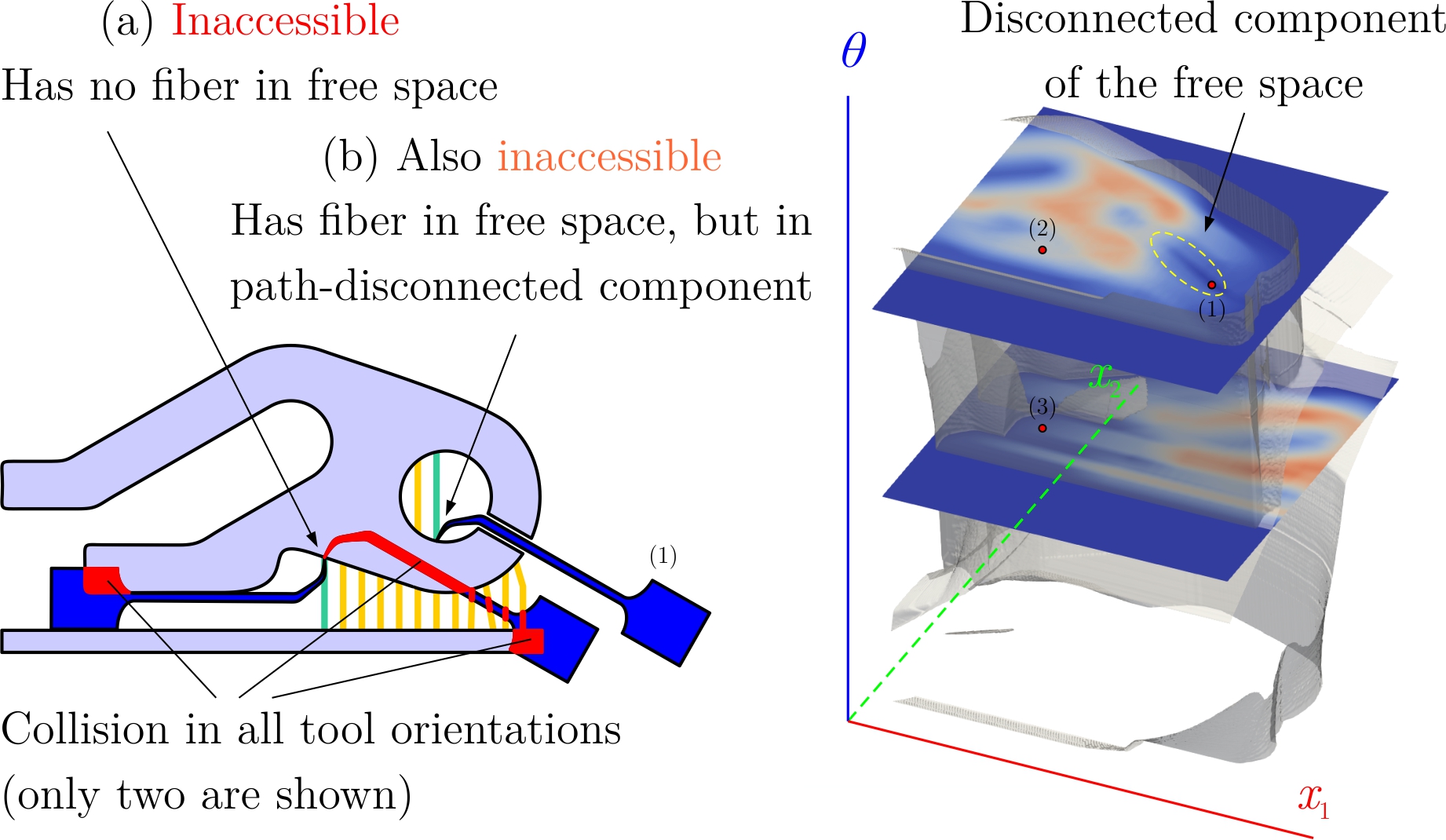
Figure 10 illustrates an example of a
false-positive. Such scenarios are rare if the support structure is
designed properly.
The test provided by Algorithm [alg_removal]
is a necessary but not sufficient condition for manufacturability
because it does not consider the path-connectedness of the free
configuration space. If the free space is not path-connected, it is
possible (but rare) for dislocation features to have a collision-free
orientation that is not accessible through a collision-free path from an
initial configuration.
Although analyzing path-connectedness is important,
$`{\mathrm{SE}(\mathrm{d})}`$ is high-dimensional for
$`\mathrm{d}\geq 3`$ and the free space topology can be highly complex.
As opposed to reasoning about the topology, we can use a sampling-based
motion planner (e.g., based on probabilistic roadmaps ) to find a
collision-free path from a reasonable starting configuration in
$`(\mathcal{O}(N,T))^c`$ to at least one configuration in the fiber.
The copyright of this content belongs to the respective researchers. We deeply appreciate their hard work and contribution to the advancement of human civilization.
For the moment, we take the existence of such a path for granted,
which is not always the case. We return to this issue in Section
5.2. ↩︎
The Minkowski sum of two pointsets
$`A,B \subseteq {\mathds{R}}^\mathrm{d}`$ is defined as
$`(A\oplus B) = \{{\mathbf{a}}+ {\mathbf{b}}~|~ {\mathbf{a}}\in A ~\text{and}~ {\mathbf{b}}\in B \}`$. ↩︎
The indicator function of a pointset
$`\Omega \subseteq {\mathds{R}}^\mathrm{d}`$ at a query point
$`{\mathbf{x}}\in {\mathds{R}}^\mathrm{d}`$ is defined as
$`{\mathbf{1}}_\Omega({\mathbf{x}}) = 1`$ if $`{\mathbf{x}}
\in \Omega`$ and $`{\mathbf{1}}_\Omega({\mathbf{x}}) = 0`$ if
$`{\mathbf{x}}\not\in \Omega`$. ↩︎
The Fourier transform of convolution is the same as the product of
Fourier transforms. Hence, the convolution can be computed by two
forward transforms, one pointwise multiplication in frequency
domain, and an inverse transform. ↩︎
$`\mathcal{P}(\Omega) = \{ \Omega' ~|~ \Omega' \subseteq \Omega \}`$
denotes the powerset of a set $`\Omega`$. ↩︎
Note that superscripts here are used to indicate the rounds of the
algorithm, and should not be confused with the subscripts used
earlier to indicate connected components. ↩︎