Optimizing a Supply-Side Platforms Header Bidding Strategy with Thompson Sampling
📝 Original Paper Info
- Title: Optimization of a SSP s Header Bidding Strategy using Thompson Sampling- ArXiv ID: 1807.03299
- Date: 2018-07-11
- Authors: Gr egoire Jauvion, Nicolas Grislain, Pascal Sielenou Dkengne (IMT), Aur elien Garivier (IMT), S ebastien Gerchinovitz (IMT)
📝 Abstract
Over the last decade, digital media (web or app publishers) generalized the use of real time ad auctions to sell their ad spaces. Multiple auction platforms, also called Supply-Side Platforms (SSP), were created. Because of this multiplicity, publishers started to create competition between SSPs. In this setting, there are two successive auctions: a second price auction in each SSP and a secondary, first price auction, called header bidding auction, between SSPs.In this paper, we consider an SSP competing with other SSPs for ad spaces. The SSP acts as an intermediary between an advertiser wanting to buy ad spaces and a web publisher wanting to sell its ad spaces, and needs to define a bidding strategy to be able to deliver to the advertisers as many ads as possible while spending as little as possible. The revenue optimization of this SSP can be written as a contextual bandit problem, where the context consists of the information available about the ad opportunity, such as properties of the internet user or of the ad placement.Using classical multi-armed bandit strategies (such as the original versions of UCB and EXP3) is inefficient in this setting and yields a low convergence speed, as the arms are very correlated. In this paper we design and experiment a version of the Thompson Sampling algorithm that easily takes this correlation into account. We combine this bayesian algorithm with a particle filter, which permits to handle non-stationarity by sequentially estimating the distribution of the highest bid to beat in order to win an auction. We apply this methodology on two real auction datasets, and show that it significantly outperforms more classical approaches.The strategy defined in this paper is being developed to be deployed on thousands of publishers worldwide.💡 Summary & Analysis
This paper focuses on the optimization of a Supply-Side Platform's (SSP) header bidding strategy in competition with other SSPs for ad space. The authors propose and experimentally validate a new methodology that combines Thompson Sampling, a Bayesian approach, with particle filtering to handle non-stationarity. Classical multi-armed bandit strategies were found inefficient due to the correlated nature of the arms.The key issue tackled is how an SSP can optimize its bidding strategy in real-time auctions where multiple SSPs compete for ad space. Traditional approaches like UCB and EXP3 did not provide satisfactory results, especially when dealing with consecutive auctions due to their slow convergence rates.
To address this, the authors introduced a version of Thompson Sampling that takes into account the correlated nature of the auction arms. This Bayesian method was combined with particle filtering to handle non-stationarities in the data, allowing for sequential estimation of the highest bid needed to win an auction. The methodology’s effectiveness was demonstrated through experiments on two real datasets, showing superior performance compared to traditional methods.
The significance of this work lies in its ability to provide a more efficient and adaptable bidding strategy for SSPs, which can lead to increased revenue and improved market competitiveness. By handling non-stationarities effectively, the proposed method ensures that SSPs can adapt quickly to changing market conditions and optimize their bids accordingly.
📄 Full Paper Content (ArXiv Source)
Real-Time Bidding (RTB) is a mechanism widely used by web publishers to sell their ad inventory through auctions happening in real time. Generally, a publisher sells its inventory through different Supply-Side Platforms (SSPs), which are intermediaries who enable advertisers to bid for ad spaces. A SSP generally runs its own auction between advertisers, and submits the result of the auction to the publisher.
There are several ways for the publisher to interact with multiple SSPs. In the typical ad selling mechanism without header bidding, called the waterfall mechanism, the SSPs sit at different priorities and are configured at different floor prices (typically the higher the priority, the higher the floor price). The ad space is sold to the SSP with the highest priority who bids a price greater than its floor price.
With header bidding, all the SSPs are called simultaneously thanks to a piece of code running in the header of the web page. Then, they compete in a first-price auction which is called the header bidding auction thereafter. In this mechanism, a SSP with a lower priority can purchase the ad if it pays more than a SSP with a higher priority. Consequently, a RTB market with header bidding is more efficient than the waterfall mechanism for the publisher.
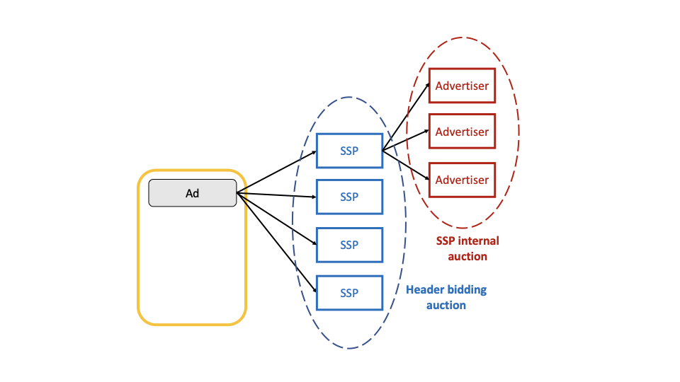
In this paper, we take the viewpoint of a single SSP buying inventory in a RTB market with header bidding. Based on the result of the auction it runs internally, it submits a bid in the header bidding auction and competes with the other SSPs. This ad-selling process is summarized on Figure 1. When it wins the header bidding auction, the SSP is paid by the advertiser displaying its ad, and pays to the publisher the closing price of the header bidding auction. We study the problem of sequentially optimizing the SSP’s bids in order to maximize its revenue. Quite importantly we consider a censored setting where the SSP only observes if it has won or lost once the header bidding auction has occurred. The bids of the other SSPs are not observed.
 />
/>
Typically some digital content will call a Supply-Side Platform (SSP) when loading, that will itself call many advertisers for bids in a real-time auction. To increase competition, some publishers have been calling several SSPs to introduce some competition among them. This setting is called header bidding because the competition among SSPs has typically been happening on the client side, in the header of HTML pages. Header bidding is, in practice, a two-staged process, with several second-price auctions happening in various SSPs, the response of which are aggregated in a final first-price auction. A SSP may be willing to adjust the bid it is responding to adapt to the first price auction context. This can be seen as an adaptative fee.
This optimization problem is formalized as a stochastic contextual bandit problem. The context is formed by the information available before the header bidding auction happens, including the result of the SSP internal auction. In each context, the highest bid among the other SSPs in the header bidding auction is modeled with a random variable and is updated in a bayesian fashion using a particle filter. Therefore, the reward (i.e., the revenue of the SSP) is stochastic. We design and experiment a version of the Thompson sampling algorithm in order to optimize bids in a sequence of auctions.
The paper is organized as follows. We discuss earlier works in Section 8. In Section 9 we formalize the optimization problem as a stochastic contextual bandit problem. We then describe our version of the Thompson sampling algorithm in Section 10. Finally, in Section 11, we present our experimental results on two real RTB auction datasets, and show that our method outperforms two more traditional bandit algorithms.
Related work
provides a very clear introduction to the header bidding technology, and how it modifies the ad selling process in a RTB market.
Bid optimization has been much studied in the advertising literature. A lot of papers study the problem of optimizing an advertiser bidding strategy in a RTB market, where the advertiser wants to maximize the number of ads it buys as well as a set of performance goals while keeping its spend below a certain budget (see and references therein). and state the problem as a control problem and derive methods to optimize the bid online. In , the authors define a functional form for the bid (as a function of the impression characteristics) and write the problem as a constrained optimization problem.
The setting of an intermediary buying a good in an auction and selling it to other buyers (which is what the SSP does in our setting) has been widely studied in the auction theory literature. In , the author uses the tools developed in (one of the most well-known papers in auction theory) to derive an optimal auction design in this setting, and and analyze how the intermediary should behave to maximize its revenue.
studies the optimal mechanism a SSP should employ for selling ads and analyzes optimal selling strategies. analyzes the optimal behaviour of a SSP in a market with header bidding, and validates the approach on randomly generated auctions.
From an algorithmic perspective, the Thompson sampling algorithm was introduced in . The papers studied its theoretical guarantees in parametric environments, while studied it in non-parametric environments. Besides, a very clear overview of the particle filtering approach to update the posterior distribution is given in .
Bandit algorithms were already designed and studied for repeated auctions, including RTB auctions. For instance, in repeated second-price auctions, construct a bandit algorithm to optimize a given bidder’s revenue, while design a bandit algorithm to optimize the seller’s reserve price.
In a setting very similar to ours, study the situation where a given SSP competes with other SSPs in order to buy an ad space. They design an algorithm that provably enables the SSP to win most of the auctions while only paying a little more than the expected highest price of the other SSPs. Though the problem seems similar, our objective is different: we want the SSP to maximize its revenue, and not necessarily to win most auctions with a small extra-payment. In particular we cannot neglect the closing price of the SSP’s internal auction in the optimization process.
We finally mention the work of for the online posted-price auction: for each good in a sequence of identical goods, a seller chooses and announces a price to a new buyer, who buys the good provided the price does not exceed their private valuation (see also when the seller faces strategic buyers). Though their problem is different, the shape of their reward function is very similar to ours. The authors show that the classical UCB1 and Exp3 bandit algorithms applied to discretized prices are worst-case optimal under several assumptions on the sequence of the buyers’ valuations. In our paper we do not tackle the worst case and instead use prior knowledge on the ad auction datasets (i.e., an empirically-validated parametric model) to better optimize the SSP’s revenue.
Problem statement
RTB market
We represent the RTB market as an infinite sequence $`\mathcal{D}`$ of time-ordered impressions $`1,\ldots,n,\ldots`$ happening at times $`t_1,\ldots,t_n,\ldots`$. We note $`\mathcal{D}_t`$ the sequence of impressions happening before time $`t`$ (including $`t`$).
Impression $`i`$ happening at time $`t_i`$ is characterized by a context $`c_i`$, which summarizes all the information relative to impression $`i`$ that is available before the header bidding auction starts. It may contain the ad placement (where it is located on the web page), some properties of the internet user (for example its operating system), or the time of the day. An important variable of the context which is specific to our setting is the closing price of the SSP internal auction, which is known before the header bidding auction happens.
We assume that the context is categorical with a finite number of categories $`C`$. A continuous variable can be discretized to meet this assumption. Without loss of generality, we assume that the categories are $`1,\ldots,c,\ldots,C`$. We note $`\mathcal{D}_{t,c}`$ the subsequence of $`\mathcal{D}_t`$ containing all impressions $`i`$ such that $`c_i=c`$.
Ad selling process with header bidding
We assume that $`S`$ SSPs: $`\mathcal{S}_1,\ldots,\mathcal{S}_S`$ compete in the header bidding auctions (possibly bidding $`0`$ if they are not interested in purchasing the ad). We note $`b_{i,s}`$ the bid of $`\mathcal{S}_s`$ in the header bidding auction for impression $`i`$. As the header bidding auction is a first-price auction, its closing price is $`\max_s(b_{i,s})`$.
From now on, we consider the problem from $`\mathcal{S}_1`$ standpoint. We note $`q_i = b_{i,1}`$ the bid submitted by $`\mathcal{S}_1`$ in the header bidding auction, which is the variable to optimize. We also write $`x_i = \max(b_{i,2},\ldots,b_{i,S})`$, which is the highest bid among the other SSPs.
In each impression $`i`$, we assume that $`\mathcal{S}_1`$ runs an internal auction between advertisers, whose closing price is denoted $`p_i`$. $`p_i`$ is the amount paid by the advertiser winning the internal auction to $`\mathcal{S}_1`$ should $`\mathcal{S}_1`$ win the header bidding auction. Note that we do not need to know the detailed internal auction mechanism but only its closing price.
Before header-bidding, a SSP would run a second-price auction with an
advertiser bidding $10 and closing at $`p_i = \$8$. Then the SSP would respond $q_i = p_i - \text{fees} = $6$ to the publisher. In this context, the advertiser pays $$8$, the publisher receives $$6$ and the SSP gets its fees: $$2`$. In a header bidding context, the SSP is
in competition with other SSPs in a first price auction, it may lose an
opportunity by taking too much fees or pay too much if it is sure to win
and take too little fees.
Revenue function for the SSP $`\mathcal{S}_1`$
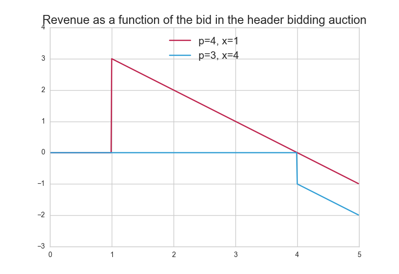
The revenue function $`R_i(.)`$ of $`\mathcal{S}_1`$ at impression $`i`$ can be written as $`R_i(q) = \mathbf{1}_{q \geq x_i}(p_i - q)`$. Indeed:
-
When $`q \geq x_i`$, $`\mathcal{S}_1`$ wins the header bidding auction. It is paid $`p_i`$ by the advertiser winning the internal auction, and it pays $`q`$ to the publisher.
-
Otherwise, $`\mathcal{S}_1`$ does not display any ad and gets no revenue in the auction.
In Figure 2 we plot $`\mathcal{S}_1`$’s revenue as a function of its bid $`q`$, for two sets of values for the closing price $`p`$ of the internal auction and the highest bid $`x`$ among the other SSPs.
Note that in the setting described here, we ignore some factors having an impact on $`\mathcal{S}_1`$’s revenue. Indeed $`\mathcal{S}_1`$ may charge a fee to the advertiser in addition to the closing price of the internal auction it runs. Also, the cost of running the internal auction may lower $`\mathcal{S}_1`$’s revenue. These factors would impact the revenue function but the strategy described in this paper would remain applicable.
Optimization problem statement
Before the header bidding auction for impression $`i`$ happens, the value $`x_i`$ of the highest bid among the other SSPs is unknown and is modeled with the random variable $`X_i`$. Thus, the revenue optimization problem over $`n`$ impressions can be expressed as follows:
\begin{equation}
\begin{split}
& \max_{q_1,\ldots,q_n} \mathbf{E}\left[\sum_{i=1}^n \mathbf{1}_{q_i \geq X_i}(p_i - q_i)] \right] \\
& \qquad = \max_{q_1,\ldots,q_n} \sum_{c=1}^C \sum_{i \in \mathcal{D}_{t_n,c}} \mathbf{E}[\mathbf{1}_{q_i \geq X_i}(p_i - q_i)] \,,
\end{split}
\end{equation}where the maximum is over the prices $`q_1,\ldots,q_n`$ that the SSP can choose as a function of the past observations.
It would be tempting to model the variables $`X_i`$ as independent and identically distributed within any context $`c`$, with an unknown distribution $`\phi_c`$. Under this assumption, the task presented here boils down to a contextual stochastic bandit problem. A closer look at the data, however, shows that there are significant non-stationarities in time. We explain below that our final model does address this issue, by the use of a particle filter within the bandit algorithm.
We emphasize that, after the header bidding auction for impression $`i`$ has occurred, $`\mathcal{S}_1`$ does not observe the value of the bid $`x_i`$, but only observes if it has won or lost the header bidding auction, i.e., $`\mathbf{1}_{q_i \geq x_i}`$. This censorship issue must be tackled in the optimization methodology.
Revenue optimization using Thompson sampling
In this section we present a method to sequentially optimize the bids $`q_i`$. It combines the Thompson sampling algorithm with a parametric model for the distributions $`\phi_c`$ (recall that $`\phi_c`$ is the distribution of the other SSPs’ highest bids $`X_i`$ within context $`c`$). Note that all the contexts $`c`$ are modeled independently.
Parametric estimation of $`\phi_c`$
We introduce $`f_{\theta}`$ a family of distributions parametrized with $`\theta`$, and we note $`F_{\theta}`$ the corresponding cumulative density functions. For each context $`c`$, we assume that the distribution $`\phi_c`$ of the other SSPs’ highest bids $`X_i`$ belongs to the family $`f_{\theta}`$; let $`\theta_c`$ be such that $`\phi_c = f_{\theta_c}`$.
According to the Thompson sampling method, we fix a prior distribution $`\pi_{c,0}(\theta)`$ over $`\theta_c`$. Then, for all $`t`$, we consider the posterior distribution $`\pi_{c,t}(\theta)`$ given all the observations available at the end of the $`t`$-th auction, i.e., the censored observations $`\mathbf{1}_{q_i \geq x_i}`$ for $`i \in \mathcal{D}_{t,c}`$.
The Bayes rule yields the following expression for $`\pi_{c,t}`$:
\begin{equation}
\pi_{c,t}(\theta) \propto \pi_{c,0}(\theta) \prod_{i \in \mathcal{D}_{t,c}} \big[F_{\theta}(q_i) \mathbf{1}_{x_i \leq q_i} + (1 - F_{\theta}(q_i)) \mathbf{1}_{x_i > q_i}\big]
\end{equation}Overview of the methodology
In our model the Thompson sampling algorithm unfolds as follows: before any impression $`i`$,
-
Sample a value $`\theta`$ from the posterior distribution $`\pi_{c_i,t_{i-1}}`$;
-
Compute the bid $`q_i`$ that would maximize the SSP’s expected revenue if $`X_i \sim f_{\theta}`$ (see below);
-
Observe the auction outcome $`\mathbf{1}_{q_i \geq x_i}`$ and update the posterior $`\pi_{c_i,t_{i}}`$.
As the particle filter provides a discrete approximation of the posterior distribution, the sampling step is straightforward. The optimization of the bid $`q_i`$ is a one-dimensional optimization problem: when $`X_i \sim f_{\theta}`$, the maximal SSP expected revenue is
\max_q (p_i - q) F_{\theta}(q)\;.There is no closed form solution in general, but this problem can be solved numerically for example by using Newton’s method.
The difficult step of the algorithm is the update of the posterior, which is explained in the next section.
Updating the posterior distribution
It would be difficult to sample directly from the posterior distribution $`\pi_{c,t}`$, which does not have a simple or tractable form. Even the use of MCMC methods like Metropolis-Hastings would be hazardous, since computing the density of the posterior distribution has a linear cost in the number of past observations which is huge in advertising 1.
To overcome these difficulties, we approximate the posterior distribution with a particle filter, a powerful sequential Monte-Carlo method for Hidden Markov Models (HMM). For an introduction on HMM and particle filtering, we refer to . The basic idea of a particle filter is to approximate the sequence of posterior distributions by a sequence of discrete probability distributions which are derived from one another by an evolution procedure (which may include a selection step). The posterior distribution $`\pi_{c,t}`$ is estimated by a discrete distribution on $`K`$ points called particles. The particles are denoted by $`(\theta_{c,1,t},\ldots,\theta_{c,K,t})`$ and their respective weights by $`(w_{c,1,t},\ldots,w_{c,K,t})`$. The evolution procedure and the selection step we use are described below.
A very important strength of the particle filter approach is that it allows to handle non-stationarity: the HMM model encompasses the possibility that the hidden variable (here, the unknown parameter $`\theta`$) evolves in time according to a Markovian dynamic of kernel $`p(\theta'|\theta)`$, thus forming an unobserved sequence $`(\theta_t)_t`$. We use this possibility by assuming that the parameter $`\theta_t`$ is equal to $`\theta_{t-1}`$ plus a small step in an unknown direction: this permits to handle parameter drift directly inside of the model.
The theory of particle filters for general state space HMM suggests that, in cases such as ours, the particle approximations converge to the true posterior distributions of the parameter $`\theta`$ when the number of particles tends to infinity.
Evolution: updating the distribution
Recall that we run $`C`$ independent instances of Thompson Sampling, one for each context $`c`$. Next we focus on one context $`c`$ and recall how to update the particle distribution in the particle filter. To simplify the notation, we write $`t-1`$ and $`t`$ for the times of two consecutive impressions within context $`c`$, even if other contexts appeared in between.
The update consists of two steps. First the particles $`\theta_{c,k,t}`$ are sampled from a proposal distribution $`q(\theta_{c,k,t}|\theta_{c,k,t-1},\mathbf{1}_{q_t \geq x_t})`$. We then compute new unnormalized weights $`\hat{w}_{c,k,t}`$ by importance sampling:
\begin{equation}
\begin{split}
\hat{w}_{c,k,t} = \hat{w}_{c,k,t-1} & \times \big[F_{\theta_{c,k,t}}(q_t) \mathbf{1}_{x_t \leq q_t} + (1 - F_{\theta_{c,k,t}}(q_t)) \mathbf{1}_{x_t > q_t}\big] \\
& \times \frac{p(\theta_{c,k,t}|\theta_{c,k,t-1})}{q(\theta_{c,k,t}|\theta_{c,k,t-1},\mathbf{1}_{q_t \geq x_t})} \;,
\end{split}
\end{equation}where $`p(\theta'|\theta)`$ is the transition kernel of the hidden process. Here, we may simply take the proposal distribution $`q(\theta_{c,k,t}|\theta_{c,k,t-1},\mathbf{1}_{q_t \geq x_t})`$ to be equal to the transition distribution $`p(\theta_{c,k,t}|\theta_{c,k,t-1})`$, which yields:
\begin{equation}
\hat{w}_{c,k,t} = \hat{w}_{c,k,t-1} \times \big[F_{\theta_{c,k,t}}(q_t) \mathbf{1}_{x_t \leq q_t} + (1 - F_{\theta_{c,k,t}}(q_t)) \mathbf{1}_{x_t > q_t}\big] \,.
\end{equation}The normalized weights $`w_{c,k,t}`$ can be computed as:
w_{c,k,t} = \frac{\hat{w}_{c,k,t}}{\sum_{k'=1}^K \hat{w}_{c,k',t}} \;.Selection: resampling step
The basic update described previously generally fails after a few steps because of a well-known and general problem: weight degeneracy. Indeed, most of the particles soon get a negligible probability, and the discrete approximation becomes very poor. A standard strategy used to tackle this issue is the use of a resampling step when the degree of degeneracy is considered to be too high. We use the following methodology given in for resampling:
-
Compute $`S = \Big(\sum_{k=1}^K w_{c,k,t}^2\big)^{-1}`$ to quantify the degree of degeneracy of the particle filter
-
If $`S < S_{\min}`$ ($`S_{\min}`$ is a hyperparameter of the particle filter), resample all the particles by sampling $`K`$ times with replacement the current set of weighted particles $`\left\{\theta_{c,1,t},\ldots,\theta_{c,K,t}\right\}`$. The result is an unweighted sample of $`K`$ particles, so we set the new weights to $`\hat{w}_{c,k,t} = \frac{1}{K}.`$
There exist some alternative resampling schemes that could be used: see for a presentation of some of them, and for a discussion on their convergence properties and computation cost.
Time and space complexities. Recall that $`K`$ is the number of
particles and that $`C`$ is the number of contexts. After each new
impression $`i`$, since $`i`$ only falls into one context $`c`$, the
evolution and selection steps described above need only be carried out
for this particular $`c`$. This thus only requires $`\mathcal{O}(K)`$
elementary operations per impression (including calls to the cumulative
distribution function $`F_{\theta}(x)`$). As for space complexity, a
direct upper bound is $`\mathcal{O}(C K)`$ since we need to store weight
vectors for each context $`c=1,\ldots,C`$.
Implementation of Thompson sampling
We may now detail our modelling and algorithmic choices for the particle filter within the Thompson sampling algorithm.
Distribution of the highest bids $`x_i`$.
We model the highest bids $`x_i`$ among the other SSPs with a lognormal distribution, a standard choice in econometrics or finance. Lognormal distributions are parametrized by $`\theta=\left(\theta^{(1)}, \theta^{(2)} \right),`$ where $`\theta^{(1)}=\sigma>0`$ and $`\theta^{(2)}=\mu \in \mathbb{R}.`$ Here, $`\mu`$ and $`\sigma`$ are respectively location and scale parameters for the normally distributed logarithm $`\ln(x_i).`$
Particle filter.
We write $`\theta_c`$ for the parameters of the lognormal distribution associated with context $`c`$. The particle filter for the posterior distributions works as follows:
-
In order to handle non-stationarity, we model the parameters $`\theta_{c}`$ by Markov chains $`\theta_{c,t}`$ such that $`\log\left(\theta^{(1)}_{c,t}\right)=\log\left(\theta^{(1)}_{c,t-1}\right)+ E_1`$ and $`\theta^{(2)}_{c,t}=\theta^{(2)}_{c,t-1}+ E_2`$, where $`E_1,E_2\sim \mathcal{N}(0,\epsilon=0.005)`$ are independent Gaussian variables with mean $`0`$ and standard deviation $`\epsilon.`$
-
At each time $`t`$, for each context $`c\in\{1,\dots,C=100\}`$, we use $`K=100`$ particles $`\theta_{c,k,t}=\left(\theta^{(1)}_{c,k,t}, \theta^{(2)}_{c,k,t} \right).`$
-
As explained above, the particles $`\theta_{c,k}`$ evolve at step $`t`$ according to the same dynamic as the unobserved parameters $`\theta_{c,t}`$: $`\log\left(\theta^{(1)}_{c,k,t}\right)=\log\left(\theta^{(1)}_{c,k,t-1}\right)+\mathcal{N}(0,\epsilon=0.005)`$ and $`\theta^{(2)}_{c,k,t}=\theta^{(2)}_{c,k,t-1}+\mathcal{N}(0,\epsilon=0.005).`$
-
We use a uniform distribution as prior $`\pi_{c,k,0}(\theta)`$ for the parameter $`\theta_{c,0}`$, and thus uniformly generate the components of the initial particle $`\theta_{c,k,0}=\left(\theta^{(1)}_{c,k,0}, \theta^{(2)}_{c,k,0} \right).`$ Because of the high number of auctions in each context, the choice of the prior distribution $`\pi_{c,k,0}(\theta)`$ has little impact on the result, as long as its support contains the parameter $`\theta_c`$.
-
Finally, we choose $`S_{min}=K/2`$ as a resampling threshold criterion.
Experiments on RTB auctions datasets
Constrution of the datasets
In practice, the SSPs generally do not share their bids with one another, and we do not have a dataset with the bids from all SSPs in header bidding auctions. The datasets we have used in these experiments give, for two web publishers, the bids as well as the names of the advertisers in RTB auctions run by a particular SSP over one week, in a setting without header bidding.
For these two web publishers, a dataset giving both the bids in $`\mathcal{S}_1`$ internal auction and the bids from other SSPs in the header bidding auction has been artificially built the following way:
-
All the advertisers competing in the RTB auctions (typically a few dozens) have been randomly assigned to one of two groups of advertisers named A and B
-
In each auction, the bids coming from advertisers in the group A are supposed to be the bids of the internal auction run by the SSP $`\mathcal{S}_1`$, and the bids coming from advertisers in the group B are supposed to be the bids coming from the other SSPs in the header bidding auction
-
Hence, in a given auction $`i`$, the closing price of the internal auction $`p_i`$ is given by the second highest bid from advertisers in the group A, and the highest bid among other SSPs $`x_i`$ is given by the highest bid from advertisers in the group B
-
The auctions where there are less than two bids from advertisers in the group A or less than one bid from advertisers in the group B have been removed from the dataset
These two datasets are named $`P_1`$ and $`P_2`$ thereafter. A brief description is given in Table 1. We give the share of auctions where $`x_i\leq p_i`$, which is the share of auctions where the SSP $`\mathcal{S}_1`$ could have won the header bidding auction while generating a positive revenue, by choosing $`q_i \in [x_i,p_i]`$.
| $`P_1`$ | $`P_2`$ | |
|---|---|---|
| Number of auctions | 1,496,294 | 410,840 |
| Number of users | 875,634 | 269,272 |
| Number of ad placements | 3,526 | 31 |
| Share of auctions where $`x_i\leq p_i`$ | $`55.2\%`$ | $`48.4\%`$ |
Some properties of the datasets $`P_1`$ and $`P_2`$.
The experiments have been performed in the two following configurations:
-
Stationary environment: the data is shuffled. This configuration is used to evaluate the strategy in a stationary environment
-
Non-stationary environment: the data is sorted in chronological order. In this case, the data is non-stationary, as the bids highly depend on the time of the day. This configuration is used to evaluate the strategy in a non-stationary environment
Note that all the bids have been multiplied by a constant.
Definition of the contexts
In the experiments, we define the context in auction $`i`$ by the closing price of $`\mathcal{S}_1`$ internal auction $`p_i`$. The closing price $`p_i`$ is transformed into a categorical context by discretizing it into $`C`$ disjoint bins.
The $`l`$-th bin contains all auctions where $`p_i \in \left[ q(\frac{l-1}{C}), q(\frac{l}{C}) \right[`$, where $`q`$ is the empirical quantile function of the closing prices $`(p_i)`$ estimated on the data. Consequently, each one of the $`C`$ contexts contains approximately the same number of auctions.
The number of contexts should be chosen carefully. A high number of contexts enables to model more precisely the distribution of the highest bid among other SSPs, which is modeled independently on each context, at the price of a slower convergence. In the experiments, we have chosen $`C=100`$ which yields a good performance on the datasets.
Baseline strategies
We define in this section the baseline strategies used to assess the quality of the Thompson sampling strategy. They correspond to the use of classical multi-armed bandit (MAB) models . Each arm $`j=1,\ldots,J`$ corresponds to a coefficient $`\alpha^{(j)}=\frac{j}{J}`$ applied to the closing price of the internal auction $`p_i`$ to obtain the bid of the SSP $`\mathcal{S}_1`$, $`q_i = \alpha^{(j)} \cdot p_i`$. Note that this strategy implies that $`q_i \leq p_i`$, as the revenue for the SSP $`\mathcal{S}_1`$ can not be positive when $`q_i > p_i`$.
In each auction $`i`$, the SSP $`\mathcal{S}_1`$ chooses an arm $`j(i)`$ and bids $`q_i=\alpha^{j(i)} \cdot p_i`$. Then, it receives a reward equal to $`\mathbf{1}_{q_i \geq x_i}(p_i - q_i)`$, and the rewards associated to the other arms are unknown.
The goal of the SSP is to maximise their expected cumulative reward. In the MAB literature, this reward maximisation is typically defined via the minimisation of the equivalent measure of cumulative regret. The regret is the difference between the cumulative rewards of the SSP $`\mathcal{S}_1`$ and the one that could be acquired by a policy assumed to be optimal. In our case, the optimal policy (or the oracle strategy) consists in playing for each auction $`i`$ the price $`q_i=x_i\,\mathbf{1}_{\left\{x_i\leq p_i\right\}}.`$
We consider two baseline strategies, corresponding to two distinct state-of-the-art policies:
-
the Upper Confidence Bound (UCB) policy . Under the assumption that the rewards of each arm are independent, identically distributed, and bounded, the UCB policy achieves an order-optimal upper bound on the cumulative regret;
-
the Exponential-weight algorithm for Exploration and Exploitation (Exp3) policy . Without any assumption on the possibly non-stationary sequence of rewards (except for boundedness), the Exp3 policy achieves a worst-case order-optimal upper bound on the cumulative regret.
The number of arms $`J`$ has a high impact on the performance of these baseline strategies. A high number of arms makes the discretization of the coefficient applied to the bid $`p_i`$ very precise, but slows the convergence as the average reward for each arm is learnt independently. We have used $`J=100`$ in the experiments.
Evaluation of the Thompson sampling strategy
This section compares the performance of the Thompson sampling strategy (TS) defined in Sections 10 and 10.4 with the performance of the two baseline strategies (UCB and Exp3) introduced in Section 5.3 on the datasets $`P_1`$ and $`P_2`$.
The performance of a strategy after $`n`$ auctions is measured with the average reward:
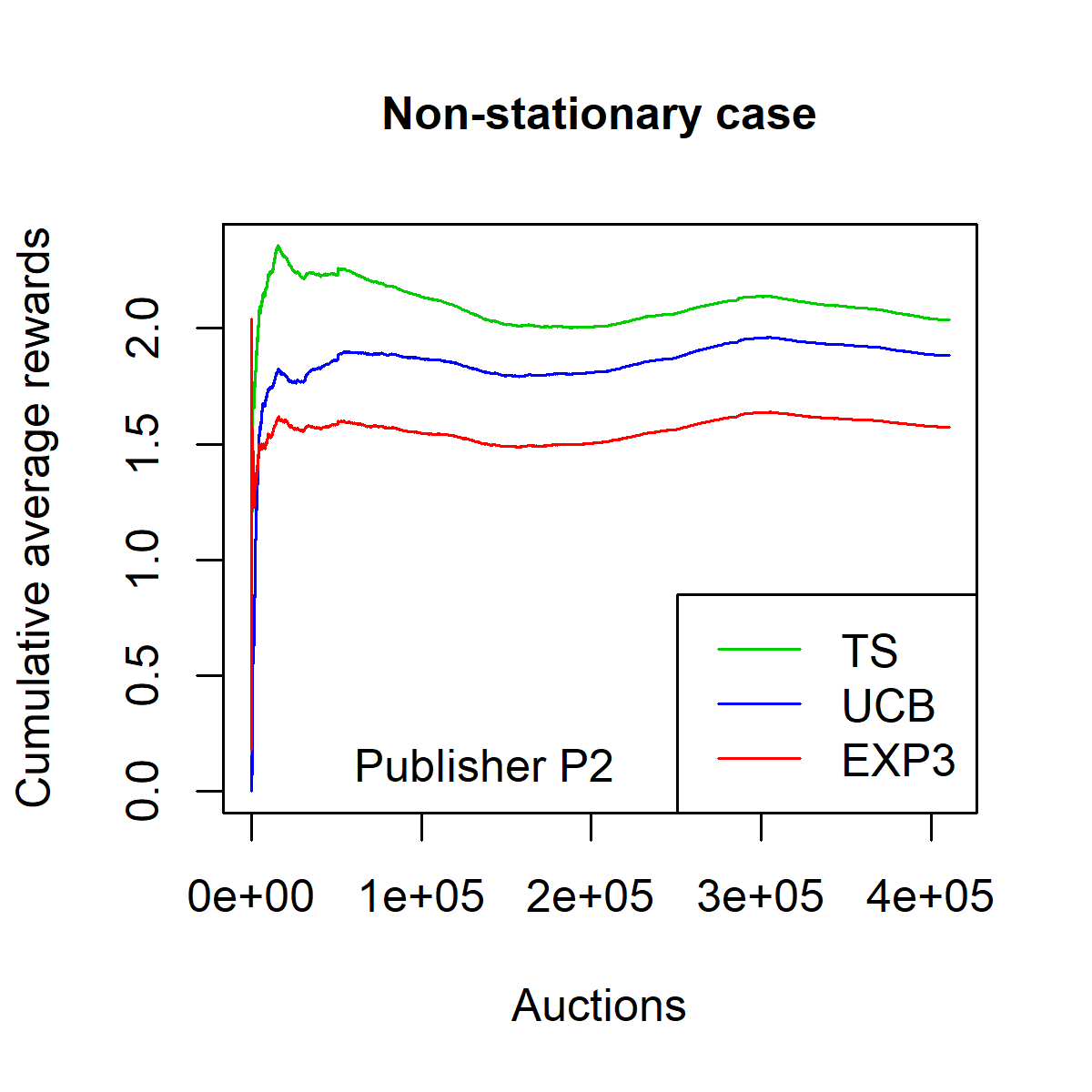
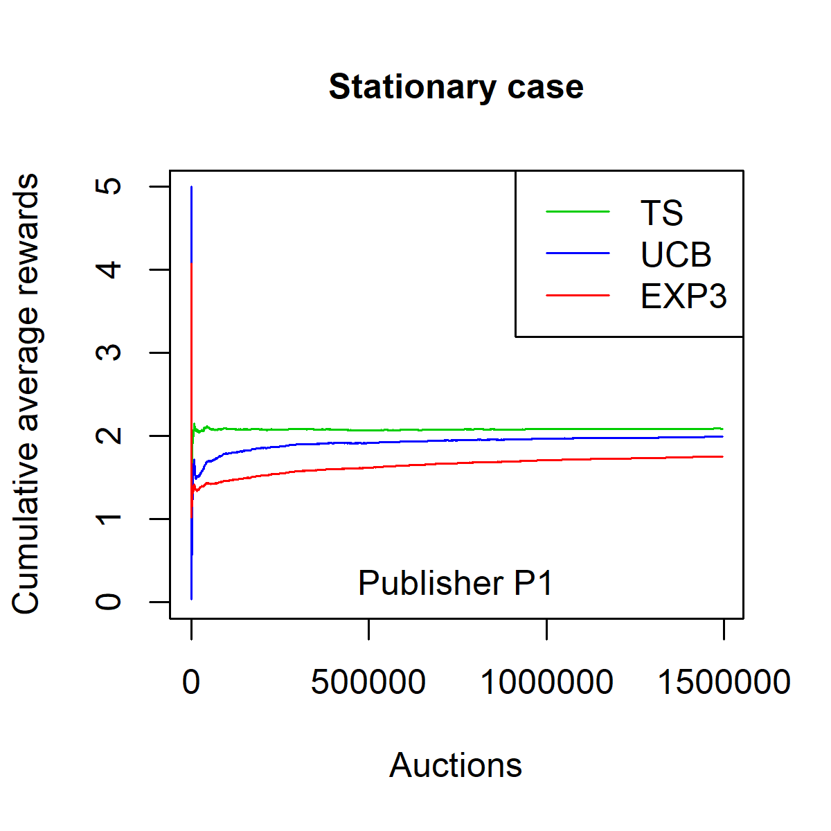
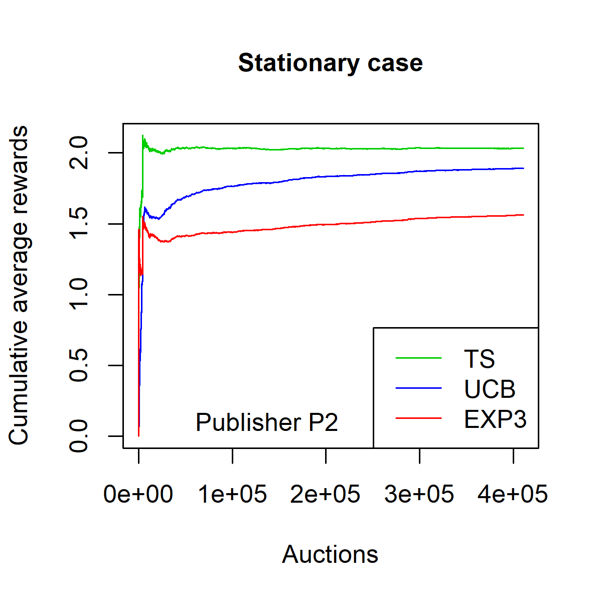
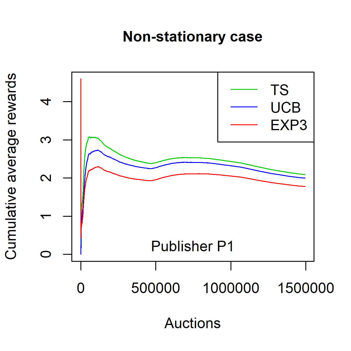
\frac{1}{n} \sum_{i=1}^n \mathbf{1}_{q_i \geq x_i} (p_i - q_i) \,.Figures [fig:fpa_3621_shuffled_models-013]-[fig:fpa_3621_sorted_model-013] plot the average reward as a function of $`n`$ on dataset $`P_1`$, in a stationary environment (i.e. on the shuffled dataset) and in a non-stationary environment (i.e. on the ordered dataset). Figures [fig:fpa_1324_shuffled_models-013]-3 plot the same results on dataset $`P_2`$.
The TS strategy clearly outperforms the baseline strategies EXP3 and UCB in both stationary and non-stationary environments. Moreover, one can observe that the convergence of the TS strategy is faster than that of the EXP3 and the UCB strategies. This convergence speed is expressed in terms of the smallest number of auctions needed by the strategy to reach the overall average reward on the whole dataset.
On the dataset $`P_1`$, the average reward with TS strategy is $`2.0888`$ for the stationary case and $`2.0937`$ for the non-stationary case. The corresponding success rates (i.e. the share of auctions won $`n^{-1} \sum_{i=1}^n \mathbf{1}_{q_i \geq x_i}`$) are $`32.19\%`$ and $`32.09\%`$ respectively.
On the dataset $`P_2`$, the average reward with TS strategy is $`2.0312`$ for the stationary case and $`2.0342`$ for the non-stationary case. The corresponding success rates are $`29.36\%`$ and $`29.10\%`$ respectively.
Advantages of the Thompson sampling strategy
The main advantage of the Thompson sampling strategy introduced in this paper is that it relies on a random modeling of the highest bid among other SSPs $`x_i`$, which is the unknown variable. Then, the revenue function of the problem is introduced explicitly to determine an optimal bid in each auction. In the strategies EXP3 and UCB, the rewards corresponding to each arm are learnt independently whereas they are highly correlated because they derive from a common revenue function.
In addition, as argued above, the use of a particle filter within Thompson sampling permits to handle elegantly a parameter drift, a problem which is still under investigation for classical bandit algorithms. We ran experiments using the non-stationary bandits algorithms of , but the results were not better than plain UCB strategies. In contrast, the algorithm proposed above significantly outperforms the classical approaches.
The price for this improvement is an increased computational cost (proportional to the number of particles), and the presence of an additional parameter $`\epsilon`$ which controls the intensity of the drift. It must be chosen so as to reach a good tradeoff between accuracy of the discrete approximation and the adaptation to the parameter drift. Experiments show, however, that even a very rough choice of $`\epsilon`$ does lead to good performance, and that over-estimating the drift intensity has little impact.
Discussion on the parameters of the Thompson sampling strategy
Choice of the contexts
As precised in Section 11.2, the number of contexts has a high impact on the performance of the strategy and should be chosen carefully.
In the experiments presented in this paper, we have defined the context as the closing price of the internal auction run by the SSP $`\mathcal{S}_1`$. This definition of the context is intuitively a good choice, as the result of the internal auction measures the value of the ad space being sold according to the advertisers bidding in this auction. This value is probably highly correlated with the bids of other SSPs for this ad space.
The definition of the contexts could be improved by using characteristics of the ad placement or of the internet user. Experiments show that defining the context as the ad placement does not improve the results.
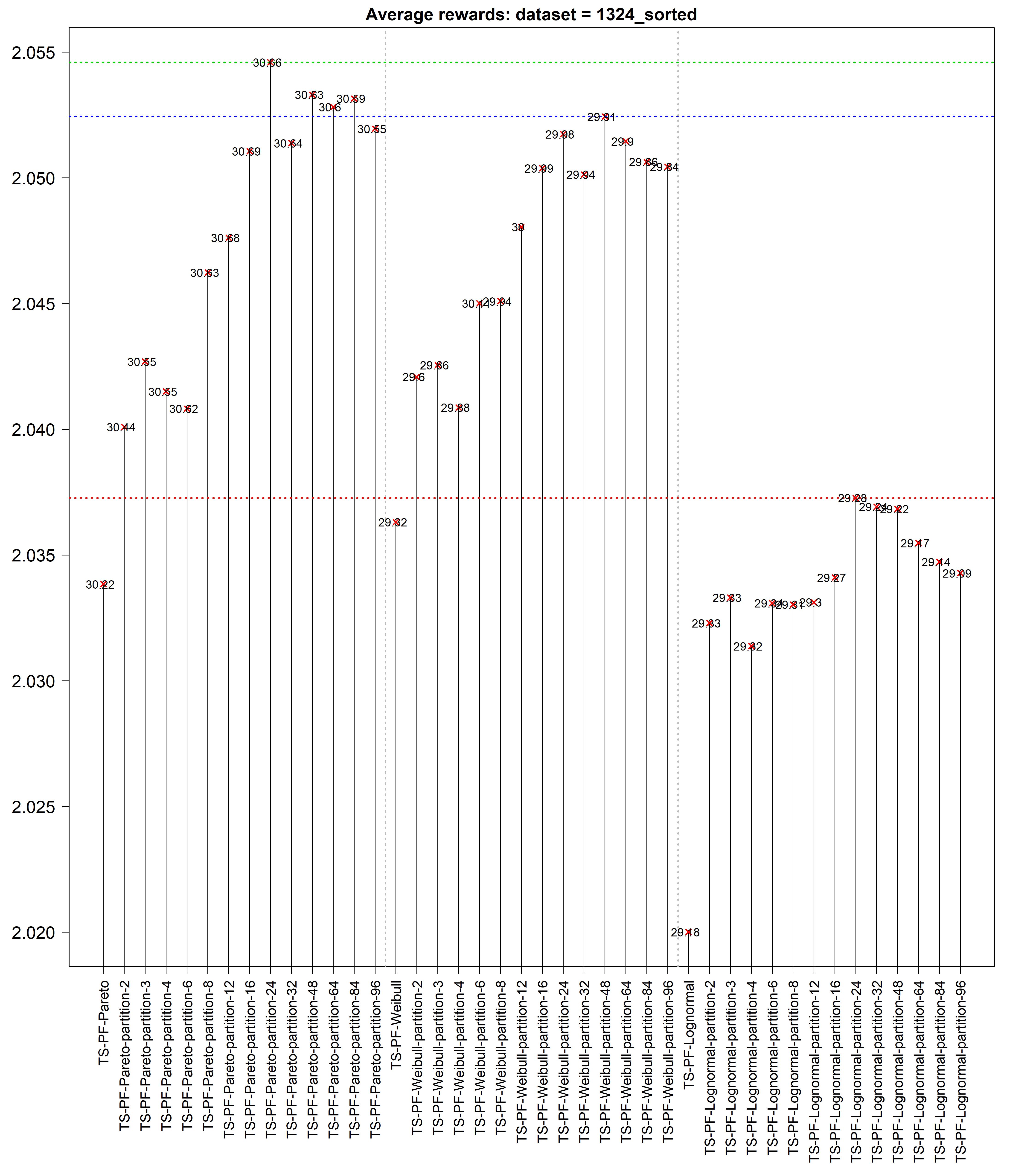
Choice of the parametric distribution
We chose the lognormal distribution to model the highest bid $`x_i`$ among the other SSPs both because it is frequently used in practice for online auctions and it fitted our datasets reasonably well. However, when the number of other SSPs is sufficiently large, using the generalized extreme value distributions or the generalized Pareto distributions might be more relevant.
Some preliminary studies we conducted show that Fréchet distributions fit well the sample maxima of the bids $`x_i`$ within each context. The reason is that such probability distributions are stable and relevant to model and to track the extreme values (sample maxima or peaks over threshold) of independent and identically distributed random variables, whatever the behavior of their tail distributions. In such situations, the associated Thompson sampling strategy could yield even higher cumulative revenues.
Computation time
We have measured the running time (the CPU response time) of the TS strategy using standard computer ($`\mu`$P $`2.8`$GHz, RAM $`8`$GB). Updating the full distribution model and estimating the optimal price $`q_i`$ for an auction $`i`$ requires about $`0.14`$ms. This running time is below the limit of $`1`$ms at which the optimal price must be decided.
Note that the running time is strongly related to the parametric probability distribution modeling the highest bid among other SSPs $`x_i`$ and to the number of particles $`K`$ used to approximate the corresponding posterior distributions.
Conclusion and future work
We have formalized the problem of optimizing the sequence of bids of a given SSP as a contextual stochastic bandit problem. This problem is tackled using the Thompson sampling algorithm, which relies on a bayesian parametric estimation of the distribution of the highest bid among other SSPs. The distribution of the highest bid among other SSPs is approximated with a particle filtering approach. It provides a very efficient way to sequentially update the distribution and sample from it to apply the Thompson sampling algorithm.
The results obtained on datasets artificially built from real RTB auctions show that the Thompson sampling strategy outperforms other bandit approaches for this problem. Also, the estimation of the optimal bid for each impression is fast enough and the strategy can be used in real conditions where a bid prediction must be performed in a few milliseconds. This strategy is currently being developed to be deployed on thousands of web publishers worldwide.
The particle filtering models naturally the non-stationarity of the bid distributions through the hypothesis $`p(\theta_{c,k,t}|\theta_{c,k,t-1})`$. This hypothesis should be linked to the non-stationarity of the distributions, as decreasing its standard deviation (named $`\epsilon`$ in the paper) enables to forget past observations faster.
In the approach described here, the contexts are modeled independently. The learning speed of the algorithm could be increased by taking into account the correlations between the contexts. In particular, these correlations may be very high when the context is defined by a continuous variable. This point may lead to improvements in the strategy.
Finally, we are planning to explore further how the performance of the strategy depends on the parametric distribution used to model the highest bid among other SSPs $`x_i`$.
📊 논문 시각자료 (Figures)
A Note of Gratitude
The copyright of this content belongs to the respective researchers. We deeply appreciate their hard work and contribution to the advancement of human civilization.-
Indeed, the profile of the payoff function induces a posterior distribution that cannot be simplified. Hence, computing the posterior density exactly, cannot be done better than by computing the product of all bayesian updates, which in practice is intractable and rules-out MCMC sampling. ↩︎