---

Hyperbolic components in spaces of polynomial maps.

arXiv:math/9202210v1 [math.DS] 22 Feb 1992Hyperbolic components in spaces of polynomial maps.J. Milnor, SUNY Stony Brook, February 1992With an Appendix by A. Poirier.Abstract.

We consider polynomial mapsf : C →C of degreed ≥2 , or moregenerally polynomial maps from a finite union of copies of C to itself which havedegree two or more on each copy. In any space PS of suitably normalized mapsof this type, the post-critically bounded maps form a compact subset CS called theconnectedness locus, and the hyperbolic maps in CS form an open set HS calledthehyperbolic connectedness locus.

The various connected components Hα ⊂HSare calledhyperbolic components. It is shown that each hyperbolic componentis a topological cell, containing a unique post-critically finite map which is calleditscenter point.

These hyperbolic components can be separated into finitely manydistinct “types”, each of which is characterized by a suitablereduced mappingschema¯S(f) . This is a rather crude invariant, which depends only on the topologyof f restricted to the complement of the Julia set.

Any two components with thesame reduced mapping schema are canonically biholomorphic to each other. Thereare similar statements for real polynomial maps, or for maps with marked criticalpoints.§1.

Introduction.First some mild generalizations of standard concepts. (See for example [D1], [DH1], [M2].) Let M bethe disjoint union of finitely many copies of the complex numbers C , and let f : M →M be a properholomorphic map, of degree at least two on each component.

The filled Julia set K(f) ⊂M is the set ofall points whose forward orbit is contained in some compact subset of M . Such a map is post-criticallybounded if every critical point is contained in K(f) , and is post-critically finite if the orbit of everycritical point is finite.

Define the fully invariant Julia 1 set J(f) to be the complement of the region in Mwhere the collection of iterates of f forms a normal family. Extending the classical theory of Fatou and Julia,it is easy to check that J(f) coincides with the topological boundary ∂K(f) .

Furthermore, the intersectionof K(f) or J(f) with each component of M is connected if and only if f is post-critically bounded.Such a map is hyperbolic (ie., hyperbolic on its Julia set) if and only if every critical orbit converges toan attracting cycle. Here a cycle (=periodic orbit) is called attracting if and only if its multiplier λ , thefirst derivative around the orbit, satisfies |λ| < 1 , so that it attracts all orbits in a neighborhood.First consider the classical and most important case M = C .

A polynomial map f : C →C of degreed is monic and centered if it has the formf(z) = zd + ad−2zd−2 + · · · + a1z + a0 .Ford≥2 ,letPd−1bethecomplex(d −1)-dimensionalaffinespaceconsistingofallpolynomialmapsfromCtoitselfwhicharemonicandcenteredofdegreed . (Caution: It might seem more natural to index such a space by the degree d .

However, for our pur-poses it will be much more convenient to index by the total number of critical points, which is d −1 .) Notethat every polynomial map from C to itself is conjugate under an affine change of variable to a map fwhich is monic and centered.

Furthermore, this f is uniquely determined up to the action of the groupG(d −1) of (d −1)-st roots of unity, where each η ∈G(d −1) acts on f ∈Pd−1 by the transformationf(z) 7→f(ηz)/η .Compare 2.7 below.By definition, the connectedness locus Cd−1 ⊂Pd−1 is the compact set consisting of all polynomialsf ∈Pd−1 for which K(f) is connected, or equivalently contains all critical points. We define the hyperbolic1 This form of the definition is actually due to Fatou rather than Julia.

In our mildly generalized context,note that the closure of the repelling periodic set as considered by Julia may well be strictly smaller thanthis fully invariant set J(f) .1

connectedness locus Hd−1 ⊂Cd−1 to be the open set consisting of all f ∈Pd−1 for which the orbits ofall critical points are not only bounded, but actually converge to attracting periodic orbits.Remarks. The connectedness locus C1 for quadratic maps, better known as the Mandelbrot set, hasbeen extensively studied by Douady and Hubbard.

The locus H1 , consisting of hyperbolic maps in C1 ,was considered somewhat earlier by Brooks and Matelski. The cubic connectedness locus C2 has beenstudied by Branner and Hubbard.

In both the quadratic and the cubic cases, an important result is that thisconnectedness locus is cellular, ie., equal to the intersection of a strictly nested family of closed topologicalcells. The corresponding statement for maps of higher degree has been proved by Lavaurs.

In all cases, itis conjectured that Hd−1 is everywhere dense in Cd−1 , and coincides with the interior of Cd−1 ; howeverthese statements have not been proved even in the simplest case d = 2 .Each connected component Hα ⊂Hd−1 is called a hyperbolic componentin Cd−1 . For degreed = 2 , each map f ∈H1 has a unique attracting periodic orbit.

Let λf be its multiplier. Douady andHubbard [D1], [DH1] have shown that every hyperbolic component Hα ⊂H1 is canonically biholomorphicto the open unit disk D under the correspondencef 7→λf ∈D .Rees [R1] has studied hyperbolic components for quadratic rational maps, and McMullen [McM] has implic-itly made a corresponding study for rational maps of arbitrary degree with connected Julia set.

This paperis concerned with the special case of polynomial maps.Section 2 will begin by defining the reduced mapping schema¯S(f) = (| ¯S| , ¯F , ¯w)associated with any hyperbolic polynomial map f . This consists of a finite set | ¯S| having one point v foreach component Wv of the interior of K(f) which contains critical points, together with a “first returnmap”¯Ffrom | ¯S| to itself, and an integer valued critical weight function, where¯w(v) ≥1 is thenumber of critical points in Wv , counted with multiplicity.

To each reduced mapping schema S thereis associated an affine space PS of polynomial mappings whose principal hyperbolic component HS0provides a standard model for hyperbolic components with schema S . This standard model has a finitegroup¯G(S) ∼= Aut(HS0 ) of automorphisms.Sections 3 and 4 show that each hyperbolic component Hα , in any space PS1 , is a topological cell,and that it contains a unique post-critically finite map, called its center point fα .

(Compare [McM],[R1].) The proof, using Douady-Hubbard surgery, shows also that every hyperbolic component with reducedschema isomorphic to S is canonically diffeomorphic to a standard model B(S) , which consists of certaincollections of Blaschke products.

The diffeomorphism is unique up to composition with an element of thegroup¯G(S) , which acts on B(S) . In particular, any two hyperbolic components with the same reducedschema are canonically diffeomorphic to each other.

Section 5 sharpens this statement by showing thatthey are canonically biholomorphic. Section 6 discusses analogous results for polynomial mappings with realcoefficients, or more generally for “real forms” of complex polynomial mappings.

Section 7 studies polynomialmappings which have been critically marked by specifying an ordered list of their critical points. It is shownthat all of the principal results carry over to the critically marked case.

The Appendix, by Alfredo Poirier,shows that every possible reduced mapping schema actually occurs as the schema associated with somecritically finite hyperbolic map f : C →C .Remark. Both the statement that each hyperbolic component is a topological cell, and the statementthat it has a preferred center point, are strongly dependent on the fact that we consider only maps withconnected Julia set.

In the case of quadratic rational maps, Rees shows that the unique hyperbolic com-ponent consisting of maps with disconnected Julia set has a more complicated topology. (Compare [M4].

)For polynomial maps outside the connectedness locus, Blanchard, Devaney and Keen describe a very richtopology within the open set consisting of hyperbolic maps for which all critical orbits escape to infinity.The present work is a fairly straightforward extension of ideas originated by Douady, Hubbard, Mc-Mullen, Rees and others. I am particularly grateful to Branner and Douady for their considerable help.§2.

The Mapping Schema of a Hyperbolic Component.2

Definition 2.1. By a mapping schemaS = (|S| , F , w)we mean:(1) a finite set |S| of points, together with(2) a function F = FS from |S| to itself, and also(3) a “weight function” w = wS which assigns an integer w(v) ≥0 called the critical weight to eachv ∈|S| .Equivalently, such a mapping schema can be represented by a finite graph with one vertex for each v ∈|S| ,and with exactly one directed edge ev leading out from each vertex v to a vertex F(v) .

By definition,the degree associated with the edge ev (or with the vertex v ) is the integer d(v) = w(v) + 1 ≥1 . Thepossibility that v = F(v) , so that ev is a closed loop, is not excluded.

The vertex v is called a “criticalpoint” if w(v) ≥1 , and a “multiple critical point” if w(v) ≥2 . The sumw(S) = Σv∈|S| w(v)is calledthe total critical weight of the schema S .3

Such a mapping schema is reduced if every vertex is critical.Suppose that we start with a notnecessarily reduced mapping schema S which satisfies the following very mild condition: Every cycle in Smust contain at least one critical point. Then there is an associated reduced schema ¯S which is obtainedfrom S simply by discarding all vertices of weight zero and shrinking every edge of degree one to a point.

(Compare Figure 1.) Note that S and¯S have the same critical weight.

In the special case where S isitself a reduced mapping schema, evidently S = ¯S .SSFigure 1.A mapping schema of total weight five, and the associated reducedschema of weight five. The heavy dots represent critical points, and the doubleheavy dots represent critical points of weight two.Each mapping schema can be conveniently described by a symbol as follows.

The symbol (w) standsfor the graph with a single vertex of weight w and a single edge which is a closed loop of degree w + 1 ,while (w1, . .

. , wk) , or any cyclic permutation of this symbol, stands for a graph with k vertices of weightsw1, .

. .

, wk arranged in a cycle. Note that every connected mapping schema contains exactly one such cycle.To indicate that additional vertices with weights w′1, .

. .

, w′m map to the vertex of weight wi , we insert theexpression {w′1, . .

. , w′m} immediately in front of the symbol wi .

Continuing this construction inductively,we obtain an appropriate symbol for any connected mapping schema. As an example, the schema S ofFigure 1 has symbol{{1, 0}0}0 , {1}1 , 0 , 2up to cyclic permutation, and the associated reduced schema¯S has symbol ({1, 1}1 , 2) .

Finally, using the notation S + S′ for a disjoint union, we obtain symbols fordisconnected schemata also. (2)(1,1)({1}1)(1)+(1)+Figure 2.

The reduced schemata of weight two.Up to isomorphism, there is just one reduced mapping schema of total weight one, with symbol (1) ;while there are four reduced schemata (2) , (1, 1) , ({1}1) , and (1) + (1) of weight two. (Compare [R1].In [M3] the letters A, B, C, D were used for these four types.) I don’t know any general formula for thenumber N(w) of distinct reduced schemata of weight w .

However, for n ≤5 this number can be computedas follows:N(1) =1N(2) =4=3 + 1N(3) = 12 =8 + 3 + 14

N(4) = 42 = 24 + 14 + 3 + 1N(5) = 138 = 72 + 48 + 14 + 3 + 1 .Here the first summand gives the number of connected schemata, the next gives the number with twocomponents, and so on. This can be proved simply by constructing an exhaustive list.Any hyperbolic polynomial map f from C to C , or from a finite union of copies of C to itself ofdegree two or more on each copy, gives rise to an associated full mapping schema S = (|S| , F , d) by thefollowing construction.

Let W(f) be the union of the basins of attraction for all attracting periodic orbitsof f in C . (Equivalently, since f is hyperbolic, W(f) is the interior of the filled Julia set.) Thus W(f)is the bounded open set consisting of all points z whose forward orbit converges to a attracting periodicorbit.

It is not difficult to check that:(a) each connected component of W(f) is simply connected, and hence is conformally isomorphic tothe open unit disk; and(b) the map f carries each component Wα of W(f) properly onto some component f(Wα) = Wβof W(f) by a map of degree dα ≥1 .Furthermore, f is bijective on a given component Wα if and only if dα = 1 , or in other words ifand only if there are no critical points in Wα . Let W PC be the union of those components Wv of W(f)which contain post-critical points of f , that is points which are either critical or belong to the forwardorbit of some critical point.Definition 2.2: The full mapping schema of f .

This schema S(f) has one vertex v corre-sponding to each post-critical component Wv ⊂W PC . The weight w(v) is defined to be the number ofcritical points in Wv , counted with multiplicity.

Each vertex v is joined to a vertex F(v) by an edge evof degree w(v) + 1 , where F(v) is the vertex associated with the component f(Wv) = WF (v) ⊂W PC .Definition 2.3: The reduced schema of f . In practice, we will always work with the associatedreduced mapping schema¯S(f) , which can be constructed from S(f) as above, or can be constructeddirectly as follows.

Let W C ⊂W PC be the union of the critical components of W(f) , that is the unionof those components Wv which contain critical points of f , and let f C : W C →W C be the first returnmap. In other words, f C(z) is equal to the first of the pointsf(z) , f ◦2(z) = f(f(z)) , f ◦3(z) = f(f(f(z))) , · · ·which belongs to a critical component of W(f) .

It follows from the classical theory of Fatou and Julia thatevery attracting periodic orbit contains at least one point of W C , so that f C is defined. By definition,the schema¯S(f) has one vertex v for each critical component Wv ⊂W C , with a directed edge leadingfrom each vertex v to the vertex¯F(v) where the first return map f C on W C carries Wv onto W ¯F (v) .The weight w(v)) ≥1 is equal to the number of critical points of either f C or f in Wv , counted withmultiplicity.Thus the total critical weight w of S(f) or of ¯S(f) is equal to the total number of critical points off , counted with multiplicity.

We will see in the Appendix that all possible reduced schemata arise in thisway: Given any reduced mapping schema S0 with total critical weight w there exists a polynomial mapf : C →C of degree d = w + 1 which is hyperbolic, with reduced schema ¯S(f) isomorphic to S0 . We willsay briefly that such an f has type S0 .If we allow mappings from a finite union of copies of C to itself, then such a map f can be constructedtrivially as follows.Definition 2.4.The universal polynomial model space.To each reduced mapping schemaS = (|S| , F , w) there is associated a complex affine space PS of polynomial maps as follows.

Form thedisjoint union |S| × C of n copies of the complex numbers C , where n is the number of vertices of S .In other words, replace each vertex of S by a copy of C . Let PS be the space consisting of all mapsf from |S| × C to itself such that the restriction of f to each component v × C is a monic centeredpolynomial map of degreed(v) = w(v) + 1 , taking values in F(v) × C .

Note that the complex dimensionof this affine space PS is equal to the total critical weight w(S) .5

Remark. The principle that the dimension of a suitably normalized space of holomorphic maps is equalto the (generic) number of critical points seems to be true in a number of interesting cases.

Here are twofurther examples. For polynomials of degree d ≥2 with just one multiple critical point, there is a normalform z 7→zd + c depending on one parameter.

On the other hand, the space of all holomorphic conjugacyclasses of rational maps f : C ∪∞→C ∪∞of degree d ≥2 has complex dimension 2d −2 , and eachsuch map has exactly 2d −2 critical points counted with multiplicity.In the special case where S is the schema (w) = (d −1) with just one vertex, clearly the space P(w)of 2.4 coincides with the space Pd−1 described in §1. For any S , the connectedness locus CS ⊂PS andthe hyperbolic set HS ⊂CS can be defined just as in the special case S = (w) .

By definition, a mapf ∈PS belongs to the connectedness locus CS if and only if its filled Julia set K(f) ⊂|S| × C intersectseach component v × C in a connected set, or if and only if every critical point has bounded orbit. Eachhyperbolic map f ∈HS will have its own reduced schema ¯S(f) .

In general, ¯S(f) will not be isomorphicto the given schema S , although it will have the same total critical weight. (Compare 2.11.

)There is a preferred base point f0 in HS , namely the unique mapf0(v , z) = (F(v) , zd(v))whose constituent polynomials are all monic monomials. Clearly the mapping schema S(f0) = ¯S(f0) asso-ciated with this central point can be identified with the given reduced schema S .

The hyperbolic componentHS0containingf0willbecalledtheprincipalhyperbolic component of CS . We will use HS0as a standard model for hyperbolic components withreduced schema isomorphic to S .Definition 2.5.

The symmetry groups G(S) →¯G(S) . By the group Aut(S) of automorphismsof the schema S = (|S| , F , w) , we mean the finite group consisting of all permutations of the set |S| ofvertices which commute with the map F and preserve the weight w(v) .

As examples, for the graphs shownin Figures 1b, 2b, and 2d, this automorphism group is cyclic of order two, but for the remaining graphs inFigures 1 and 2 it is trivial. (Compare 2.10 below.) Each such automorphism gives rise to an automorphismof the spacesHS0⊂HS ⊂CS ⊂PSwhich is linear in the sense that it preserves the affine structure and fixes the base point f0 .

However,these spaces have a possibly larger group of linear automorphisms, as follows. We first introduce the fullsymmetry group G(S) consisting of all maps g from |S|× C to itself which are bijective, commute withf0 , and carry each component v × C linearly onto some v′ × C .Lemma 2.6.

Conjugation by an element g ∈G(S) carries each polynomial map f ∈PS toa map g ◦f ◦g−1 ∈PS . The resulting action of the group G(S) on the space PS is linear,and preserves the subsets HS0 ⊂HS ⊂CS .The proof will be given below.Caution.

This action need not be effective: Some elements of G(S) may commute with all maps inPS , and hence act trivially on the space PS . We will use the notation¯G(S) for the effective symmetrygroup, that is the quotient group of G(S) which operates effectively on the spaces HS0 ⊂HS ⊂CS ⊂PS .For details, see 2.9 below.In order to justify the definition of PS and G(S) , let us note that any possible dynamical behaviorwhich can be obtained by nowhere linear polynomial maps from a finite union of copies of C to itself canalready be realized by some mapping f which belongs to an appropriate affine space PS of monic centeredpolynomials.

(This is an immediate generalization of the statement that every polynomial map C →C ofdegree d ≥2 is affinely conjugate to a monic centered map. )Lemma 2.7.

Let M be a finite union of disjoint copies of C , and letφ : M →MbeamapwhoserestrictiontoeachcopyofCisgivenbyapolynomialofdegree ≥2 . Then there is a mapping schema S , unique up to isomorphism, and a bijection6

h : M →|S|×C which is affine on each copy of C , so that the conjugate map f = h◦φ◦h−1belongs to the space PS . Furthermore, h is unique up to composition with elements of thefinite group G(S) which acts on |S|×C , and f is unique up to the action of¯G(S) on PS .The proof is easily supplied.⊔⊓To describe the group G(S) more explicitly, let m be the number of connected components of S , andlet δk be the product of the degrees around the unique cycle which is contained in the k-th component ofS .

Let δ′ be the product of all of the remaining degrees, which do not lie in cycles.Lemma 2.8. The group G(S) is finite, and splits canonically as a semi-direct product1 →N(S) →G(S) ←→Aut(S) →1 .Here Aut(S) is defined to be the group of automorphisms of S (see 2.5), while N(S) ⊂G(S)is a normal abelian subgroup of order (δ1−1) · · · (δm−1) δ′ .

This subgroup can be identified withthe group of all functions η from |S| to the unit circle which satisfy the identityη(F(v)) =η(v)d(v) .Proof of 2.8 and 2.6. Let N(S) be the subgroup consisting of those elements of G(S) which carryeach copy v×C to itself.

Then any element g ∈N(S) must have the form g(v, z) = (v , η(v)z) , where theη(v) are non-zero complex numbers. In fact, a brief computation shows that such a map g commutes withf0 if and only if the numbers η(v) satisfy the identities η(F(v)) = η(v)d(v) .

If v lies in the k-th cycleof S , then it follows easily that η(v) must be a (δk −1)-st root of unity. Evidently, the correspondencef 7→g ◦f ◦g−1 defines a linear action of the finite group N(S) on the affine space PS , preserving thesubsets HS0 , HS , and CS .

Further details will be left to the reader.⊔⊓Remark 2.9. A similar argument shows that the effective symmetry group¯G(S) can be identifiedwith the quotient G(S)/N0(S) , where N0 ⊂N is a direct sum of cyclic groups of order two, consisting ofall functions from |S| to {±1} which are trivial on the image F(|S|) , and also trivial on all vertices whichhave weight w(v) > 1 .

In other words, an automorphism g ∈G(S) of the space |S| × C commutes withevery map f ∈PS if and only if it belongs to this subgroup N0(S) . It follows that G(S) ̸= ¯G(S) if andonly if there exists a vertex of weight w = 1 which does not belong to the image F(|S|) ⊂|S| .2.10.

Examples. In the quadratic case S = (1) , the symmetry group G(1) is trivial.

For the fourschemata of weight 2, these groups can be tabulated as follows,SN(S)G(S)Aut(S)¯G(S)(2)Z/2Z/20Z/2(1, 1)Z/3order 6Z/2order 6({1}1)Z/2Z/200(1) + (1)0Z/2Z/2Z/2where G(1, 1) = ¯G(1, 1) is the dihedral group of order 6 . Here are four analogous examples, where the totalweight w can be arbitrary: For the schema S = (w) with a single vertex, the group N = G = ¯G is cyclicof order w and Aut(S) is trivial.

For the cycle S = (1, 1, . .

. , 1) of total weight w , the group Aut(S)is cyclic of order w and N(S) is cyclic of order 2w −1 , hence the group G(S) = ¯G(S) is non-abelianof order w (2w −1) .

For the schemaS = ({{· · · {{ 1} 1} · · · 1} 1} 1)with verticesv1 →v2 →· · · →vw−1 →vw ←⊃,the group Aut(S) is trivial and N = G is cyclic of order 2w−1 , while¯G is cyclic oforder 2w−2 . Finally, for the sum (1) + · · · + (1) of total weight w , the group G = ¯G = Aut(S) is thesymmetric group of order w!

and N is trivial. The proofs are not difficult.Remark 2.11.

An interesting relation between reduced mapping schemata of the same weight can bedefined as follows. Let us say that S ≻S′ if and only if the connectedness locus CS contains a hyperboliccomponent with reduced schema isomorphic to S′ .

This is clearly a reflexive relation; that is S ≻S in allcases.As an example, for the four reduced schemata of critical weight w = 2 , it is not difficult to check that thispartialorderingistransitive,andcanbedescribedasfollows.7

We have(2) ≻(1, 1) ≻(({1}1)(1) + (1) ,but no other relations, except as implied by reflexivity and transitivity. (There is an analogous partialordering for the various real forms of these hyperbolic components.

Compare 6.2, and Figures 3–5. )If S ≻S′ , where S′ = (|S′| , F ′ , w′) and S = (|S| , F , w) , then evidently there is an associated mapψ : |S′| →|S| which:(1) preserves order, in the sense that if F ′(v′1) = v′2 then some iterate of F maps ψ(v′1) to ψ(v′2) ,and(2) preserves weight, in the sense that Pψ(v′)=v w′(v′) = w(v) for each v ∈|S| .It is conjectured that S ≻S′ if and only if there exists such a map ψ .

In particular, it is conjecturedthat this relation is transitive. In many cases, a hyperbolic component Hα ⊂HS of type S′ seems to becontained in a complete copy of the connectedness locus CS′ , which is homeomorphically embedded intoCS in such a way that the principal component HS′0corresponds to Hα .

(This is a generalization ofthe Douady-Hubbard concept of “modulation” or “tuning” for quadratic maps.) Whenever this happens, itfollows that any type of hyperbolic component which occurs in CS′ must also occur in CS .

Thus, in thisspecial case, the relations S ≻S′ and S′ ≻S′′ certainly imply that S ≻S′′ .Caution. It may happen that S ≻S′ and S′ ≻S , even though S is not isomorphic to S′ .

Forexample, this is true for S = ({2}1, {1}1, 1) and S′ = ({1}1, {2}1, 1) . The proof of this statement is aneasy application of the Realization Theorem for “Hubbard forests”, as proved by Poirier [P3].8

§3. Blaschke Products and the Model Space B(S) .Henceforth, all mapping schemata will be reduced.

This section will describe a topological model, basedon Blaschke products, for hyperbolic components with mapping schema S . First recall some standard facts.Let D be the open unit disk in C .

For any a ∈D , there is one and only one conformal automorphismµa : ¯D →¯D which maps a to zero and fixes the boundary point 1, given byµa(z) = k z −a1 −¯azwithk = 1 −¯a1 −a .It is easy to check that the proper holomorphic maps from D onto itself are precisely the finite products ofthe formβ(z) = c µa1(z) · · · µad(z) ,with |c| = 1 . Here d is the degree, {a1 .

. .

, ad} are the pre-images of zero, and c = β(1) . Evidentlyevery such map β extends uniquely as a rational map from the Riemann sphere ˆC = C∪∞onto itself.

Inparticular, β extends continuously over the boundary circle ∂D . Note that the extension of β over ˆCcommutes with the inversion z 7→1/¯z .

In particular, if z0 is a fixed point or a critical point of β , then1/¯z0 is also.Lemma 3.1. A proper map β of degree d ≥2 from the unit disk onto itself induces a d-to-one covering map from the circle ∂D onto itself.

Such a map β has at most one fixedpoint in the open disk D . If there is an interior fixed point, then the induced map on ∂D istopologically conjugate to the linear map t 7→td of the circle R/Z .

In particular, in this casethere are exactly d −1 boundary fixed points. (On the other hand, if there is no interior fixed point, then there must be d + 1 boundary fixed points,counted with multiplicity.

)ProofOutline.For|z|=1 ,abriefcomputationshowsthatthelogarithmicderivatived log β(z)/d log(z) = z β′/βis a sum ofdterms,each of which is real and strictly positive.It follows easily thatβinducesacoveringmapontheboundary,andthatanyequationoftheformβ(z) = constant ∈∂Dhas exactly d distinct solutions. If there is an interior fixed point, then afterconjugating by a conformal automorphism, we may assume that the fixed point is z = 0 , so thatβ(z) = c z µa2(z) · · · µad(z) .It follows that |β′(0)| = |a2 · · · ad| < 1 and that |β(z)| < |z| for all z ̸= 0 in the open disk.

Thus this fixedpoint is attracting, and is unique within D . When there is such an interior fixed point, it is not difficultto check that the logarithmic derivative satisfies zβ′(z)/β(z) > 1 at all points of ∂D .

In other words, themap of ∂D onto itself is strictly expanding. In particular, every boundary fixed point z0 is repelling, withβ′(z0) > 1 .

Since the algebraic number of fixed points inˆC is equal to d + 1 , it then follows that thereare exactly d −1 distinct fixed points on ∂D .More explicitly, we can set up a coordinate system on ∂D as follows. Choose one of these boundary fixedpoints z0 and assign it the coordinate t(z0) = 0 .

Now assign the d preimages of z0 under β the coordi-nates t(z) = j/d , numbering in counterclockwise order around the circle from z0 . Similarly, assign the d2preimages under β◦2 the coordinates j/d2 , and so on.

Since β is expanding on ∂D , the iterated preim-ages of z0 are everywhere dense on ∂D , so this construction converges to a well defined homeomorphismt : ∂D≈→R/Z .⊔⊓Closely related is the statement that β gives rise to a preferred β -invariant measure ℓ= ℓβ on ∂D ,with the properties that ℓ(∂D) = 1 and that β maps any small interval of measure ℓ(I) = ǫ to aninterval of measure ℓ(β(I)) = ǫ d . For example ℓcan be defined by the formula ℓ(I) = limk→∞N(k)/dk ,where N(k) is the number of solutions to the equation β◦k(u) = 1 in the interval I ⊂∂D .Notethat this measure is “balanced” in the sense that each of the d components of β−1(I) has measure10

ℓ(I)/d . Evidently ℓcorresponds to the Lebesgue measure on R/Z under the conjugating homeomorphism.

(This ℓcan also be characterized as the unique invariant measure of maximal entropy.)Definition. Let β : D →D be a proper holomorphic map of degree d ≥2 .

We will say that β isboundary-rooted if its extension over ∂D fixes the point +1 , and fixed point centered if β(0) = 0 .Lemma 3.2. If φ is a proper holomorphic map of degree d ≥2 from D to itself, with a fixedpoint in the open disk D , then φ is holomorphically conjugate to a map h−1 ◦φ ◦h whichis boundary-rooted and fixed point centered.

In fact there are exactly d −1 distinct choicesfor the conjugating M¨obius automorphism h . The space B(d −1) consisting of all properholomorphic β : D →D which are boundary-rooted and fixed point centered of degree d is atopological cell of dimension 2d −2 .Proof.

Evidently h can be any M¨obius automorphism of ¯D which maps 0 to the unique interior fixedpoint of φ , and maps +1 to one of the d−1 boundary fixed points. Let Sn(C) be the n-fold symmetricproduct,consistingofunorderedn-tuples{a1 , .

. .

, an} of complex numbers.This can be identified with the complex affine space consisting ofall monic polynomials of degree n , under the correspondence{a1 , . .

. , an} 7→(z −a1) · · · (z −an) = zn −σ1zn−1 + −· · · ± σn ,where the σj are the elementary symmetric functions of {a1 , .

. .

, an} . Thus Sn(C) is homeomorphicto Cn ∼= R2n .

Since C is homeomorphic to the 2-cell D , it follows that Sn(D) is also homeomorphicto R2n . Now consider the space B(w) consisting of all boundary-rooted Blaschke products β of degreed = w + 1 which fix the origin.

We can writeβ(z) = z µa1(z) · · · µaw(z) .Evidently this space is homeomorphic to the symmetric product Sw(D) , and hence is a topological cell,homeomorphic to R2w . ⊔⊓We will also need to find a normal form for Blaschke products under one-sided composition with aM¨obius transformation.

Definition: A proper holomorphic map D →D of degree d ≥2 is criticallycentered if the sum of itsd −1(not necessarily distinct) critical points is equal to zero.Lemma 3.3. If φ : D →D is proper and holomorphic of degree d ≥2 , then there existexactly d distinct M¨obius automorphisms h : D →D for which the composition β′ = φ ◦his boundary-rooted and critically centered.

The space B′ consisting of all boundary-rooted,critically centered proper holomorphic maps of degree d is a topological cell of dimension 2d−2 .The proof will be based on the concept of “conformal barycenter” for a collection of points in the disk:Lemma 3.4. Given points c1 , .

. .

, cn in a Riemann surface Wisomorphic to D , thereexists a conformal isomorphism η : W →D , unique up to a rotation of D , which takes thecj to points η(cj) with sum η(c1) + · · · + η(cn) equal to zero.It follows that the point p = η−1(0) ∈Wis uniquely defined. Definition: This point p will be calledthe conformal barycenter of the cj .

A proof of this lemma can easily be constructed from [Douady andEarle, §2].⊔⊓Proof of 3.3. Evidently h can be any M¨obius automorphism of D which carries zero to the conformalbarycenter of the critical points of φ , and which carries +1 to one of the d points of φ−1(1) .To determine the topology of B′ , we proceed as follows.Note first that the subspace Sn( ¯D) ⊂Sn(C) , consisting of n-tuples which belong to the closed disk¯D , forms a closed 2n-cell with interiorequal to Sn(D) .

In fact, for each non-zero {a1 , . .

. , an} ∈Sn(C) consider the ray consisting of points{ta1 , .

. .

, tan} with t ≥0 . Each such ray crosses the boundary of Sn( ¯D) exactly once, and the image ofeach such ray in the space of ordered n-tuples (σ1 , .

. .

, σn) crosses the unit sphere exactly once. Hence,stretching by an appropriate factor along each such ray, we obtain the required homeomorphism from Sn( ¯D)11

to the unit disk in Cn . Using this construction we see also that the subspace of Sn(D) consisting ofunordered n-tuples with sum zero is a topological (2n −2)-cell.

Thus the set of Blaschke products of theform β(z) = µa1(z) · · · µad(z) with a1 + · · · + ad = 0 is an open topological (2d −2)-cell. It follows thatthe collection B′ of boundary-rooted, critically centered Blaschke products β′ of degree d is also an opentopological (2d −2)-cell.

For given any such β′ , by Lemma 3.4 there is a unique boundary-rooted M¨obiusautomorphism η so that β = β′ ◦η has the sum of its zeros equal to zero, and similarly given β there isa unique η so that β′ = β ◦η−1 is critically centered. ⊔⊓We will use such Blaschke products to model the map f C : W C →W C studied in 2.3.

Since W C isisomorphic to a disjoint union of open disks, let us first study proper maps from such a disjoint union toitself.Definition. To any reduced mapping schema S = (|S| , F , w) we associate the model space B(S)consisting of all proper holomorphic mapsβ : |S| × D →|S| × Dsuchthatβcarrieseachv × DontoF(v) × Dbyaboundary-rootedmapofdegreed(v) = w(v) + 1which satisfiesβ(v, 0) = (F(v) , 0)whenever v is periodic under F , and is criti-cally centered whenever v is not periodic under F .Lemma 3.5.

If the schema S has total weight w , then the model space B(S) is homeomor-phic to an open cell of dimension 2w .Proof. This follows easily from 3.2 and 3.3.

⊔⊓We next show that the various maps in B(S) serve as models for all possible dynamics which can occurwithin the basins of attracting cycles.Lemma 3.6. Let M be a disjoint union of finitely many open disks, and let φ : M →Mbe any proper holomorphic map, of degree ≥2 on each component of M , such that everyorbit under φ converges to an attracting cycle.

Then φ is holomorphically conjugate to amap which belongs to some model space B(S) . Here the schema S is uniquely determined upto isomorphism; and the number of distinct conformal isomorphisms from M onto |S| × Dwhich conjugate φ to some element of B(S) is equal to the order of the group G(S) .Proof.

We may identify the complex manifold M with Σ × D , where Σ is a finite index set. Notethat φ extends continuously over Σ × ∂D .

First consider some component σ × D which is mapped toitself by some iterate φ◦k . Let d1 · · · dk be the degree of φ◦k on this component.

Then φ◦k has a uniquefixed point inside σ ×D . After conjugating by a M¨obius automorphism of σ ×D , we may take this interiorfixed point to be the center point (σ , 0) .

Similarly, there ared1 · · · dk −1fixed points on σ × ∂D , andwe can rotate σ × ¯D so that one of these fixed points is (σ , 1) . Pushing forward, we find correspondinginterior and boundary points for each of the k disks in the cycle.

Finally we work outwards, first choosingcorresponding preferred points for each of the disks which maps immediately to a disk on this cycle, andthen continuing inductively. Details will be left to the reader.

⊔⊓We can sharpen 3.6 as follows.Lemma 3.7. The effective symmetry group¯G(S) of §2 operates smoothly on the model spaceB(S) in such a way that two maps in B(S) are conformally conjugate to each other if andonly if they belong to the same orbit under this action.

In fact this action of¯G(S) on B(S)is covered by an action of the full symmetry group G(S) on the product B(S) × |S| × D withthe following property: Each g ∈G(S) carries (β , v , z) to a triple of the form (β′ , h(v, z))where h = hg,β is a conformal automorphism of |S| × D depending on g and β , and whereβ′ = h ◦β ◦h−1 .Remark. We will see in §4 that B(S) is canonically diffeomorphic to the model hyperbolic componentHS0 .

Since ¯G(S) acts linearly on HS0 , it is hardly surprising that it operates smoothly on B(S) . However,to avoid a circular argument, we must prove this fact from scratch.12

Proof of 3.7. Since the action of the subgroup Aut(S) ⊂G(S) on B(S) and on B(S) × |S| × Dis quite easy to describe, let us concentrate on the complementary subgroup N(S) ⊂G(S) .In otherwords, we will only discuss those conformal automorphisms of |S| × D which carry each component ontoitself.

If such an automorphism h conjugates some map β ∈B(S) into another map β′ = h−1 ◦β ◦hwhich also belongs to B(S) , then evidently h must preserve center points, and hence must have the formh(v , z) = (v , ηv z) . (Here h is the inverse of the map considered in the previous paragraph.) Now thecondition that β′ is boundary-rooted takes the formβ(v , ηv) = (F(v) , ηF (v)) .

(1)Evidently this condition depends on the particular map β we have chosen. However, it is not difficult tocheck that the possible solutions vary continuously as we vary β .

Since the space B(S) is contractible,this means that if we find a solution for one point β0 ∈B(S) , then we obtain corresponding solutions forall points β ∈B(S) . Define the “center point” β0 ∈B(S) to be the mapping defined byβ0(v, z) = f0(v, z) = (F(v) , zd(v)) .

(2)(Compare 2.4 and 3.8.) Then it is true, almost by definition, that the group consisting of all holomorphicconjugacies from β0 to itself can be identified with the symmetry group G(S) .Thus, deforming thesolutions of (1) continuously, we obtain an action of the group N(S) , and hence of G(S) , on the spaceB(S) and on B(S) × |S| × D .Next we must ask which elements of the group N(S) ⊂G(S) act trivially on B(S) .

Note that theautomorphism h(v, z) = (v , ηv z) of |S| × D commutes with the map β(v, z) = (F(v) , βv(z)) if and onlyifβv(ηv z) = ηF (v)βv(z) . (3)In most cases, we can choose each map βv so that its set of zeros admits no non-trivial rotation.

Wheneverthis is the case, the equation (3) admits only the trivial solution ηv = ηF (v) = 1 . However, in the special casewherethevertexvhasweightw(v) = 1 , and is not periodic under F , the map βvmust be critically centered of degree two, andhence must have the formβv(z) = µa(z)µ−a(z) =z2 −a21 −¯a2z2 .In this special case, the set of zeros of βv necessarily admits an 180◦rotation.

Hence equation (3) admitsthe solutions ηv = ±1 , ηF (v) = 1 . In this way, it is not difficult to check that the subgroup N0(S) ⊂G(S)of 2.9, which acts trivially on PS , is precisely equal to the subgroup which acts trivially on B(S) .

Thuswe obtain the required effective action of the quotient group¯G = G/N0 on B(S) . The details of thisargument are not difficult, and will be left to the reader.

⊔⊓Finally, we will need the following result, which is essentially well known.Lemma 3.8. Each model space B(S) contains one and only one map β0 which is post-critically finite.

It is given by formula (2) above, and is characterized by the properties thateach component v × D contains exactly one critical point, and that β0 maps critical pointsto critical points.Proof. First consider a proper holomorphic map β : D →D , which has a attracting fixed point atzero.

If the multiplier λ = β′(0) is non-zero, then by the Kœnigs linearization theorem we can choose alocal coordinate ζ in a neighborhood of zero so that β corresponds to the map ζ 7→λζ . Let us extendthis coordinate system to a conformal isomorphism between an open set U ⊂D and an open disk |ζ| < r ,with r as large as possible.

Note that r cannot be infinite, since no open subset of D is conformallyisomorphic to the whole complex line. If r is maximal, then there must be some obstruction to extendingfurther, and this obstruction can only be a critical point lying on the boundary of U .

Thus, under thishypothesis, there must be a critical point in D whose forward orbit is not eventually periodic.Therefore, in the post-critically finite case, the multiplier λ must be zero. Suppose then that λ = 0 .By B¨ottcher’s theorem, we can choose the local coordinate ζ so that β corresponds to the map ζ 7→ζkfor some k ≥2 .

Again we extend to a conformal isomorphism from U ⊂D onto the open disk |ζ| < r13

with r as large as possible. If the maximal r satisfies r < 1 , then again there must be a critical point onthe boundary of U , whose forward orbit is not eventually periodic.

Thus, if all critical orbits are eventuallyperiodic, it follows that r = 1 . But then the boundary of U maps into itself under β , and it followseasily that U = D , so that β is conformally conjugate to the map z 7→zk .

In fact if β(1) = 1 thenβ(z) = zk . In this case, note that the unique critical point of β is the only point of D whose forwardorbit is eventually periodic.To complete the proof, we must also consider the case of a critically centered Blaschke product β : D →D , with β(1) = 1 .

If all of the critical points of β map to zero, then we must show again that β(z) = zd .But this is clear, since D is exhibited as a branched covering of D with unique branch point at the criticalvalue zero.⊔⊓§4. Hyperbolic Components are Topological Cells.The object of this section is to prove the following two results.Theorem 4.1.

If Hα ⊂CS0 is any hyperbolic component whose elements f have reducedmapping schema ¯S(f) isomorphic to S , then Hα is diffeomorphic to the model space B(S) .This diffeomorphism is canonically defined, up to composition with an element of the group¯G(S) which acts on B(S) .The proof will also demonstrate the following.Corollary 4.2 (McMullen). Each hyperbolic component Hα contains one and only one mapfα which is post-critically finite.Equivalently, such a “center” map fα has the property that each component of the complement ofJ(fα) contains one and only one pre-critical point.To begin the argument, suppose that f is a hyperbolic map belonging to some connectedness locusCS0 , with reduced mapping schema¯S(f) isomorphic to S .

Then the open set W C ⊂K(f) , as definedin 2.3, satisfies the hypothesis of Lemma 3.6. That is, W C is a union of finitely many components, eachconformally isomorphic to D , and the first return map f C from W C to itself has degree at least two oneach component.

Hence, by 3.6, there exists a conformal isomorphism h : W C →|S| × D which conjugatesf C to some map β ∈B(S) .However, we must be careful since h and β are not uniquely defined. (Compare 3.7.) To deal with thisnon-uniqueness,weproceedasfollows.NotefirstthatforeachcomponentWα ⊂W Cthe closure¯Wα is homeomorphic to the closed unit disk¯D , in a homeomorphism whichis conformal throughout the interior.

(See [DH1, pp. 13, 24, 26].)Caution.

The closed disks¯Wv are not always disjoint from each other, so the closure of W C need notbe homeomorphic to |S| × ¯D . Since boundary points of W C will play an important role in our discussion,it will be convenient to introduce the following notation.

LetˆW C = ` ¯Wv be the disjoint union of theclosures of the components of W C , and letˆf C : ˆW C →ˆW C be the continuous extension of f C .In order to choose some specific conformal isomorphism between |S| × D and W C , we must firstchoose some isomorphism ι : S →¯S(f) . Evidently the number of ways of doing this is equal to the order ofthe automorphism group Aut(S) .

For each component Wι(v) of W C , we must then choose one boundarypoint q(v) which will correspond to the boundary base point (v, 1) ∈v × ¯D . These boundary points areto be chosen as follows.Definition 4.3.

Boundary markings. Let f ∈HS0 be a hyperbolic map with reduced schema ¯S(f)isomorphic to S .

By a boundary marking q : |S| →∂ˆW C of f , covering the isomorphism ι : S →¯S(f) , we will mean a function which assigns to each vertex v ∈|S| a boundary point q(v) ∈∂Wι(v) , satisfy-ingtheconditionthatˆf C(q(v)) = q(F(v)) .14

Lemma 4.4. Such boundary markings always exist.

In fact, the number of distinct boundarymarkings for fis precisely equal to the order of the symmetry group G(S) .Given sucha boundary marking q , there is one and only one homeomorphismˆq : |S| × ¯D∼=−→ˆW C ,conformal throughout the interior, which satisfies ˆq(v, 1) = q(v) , for which the mapβ=ˆq−1 ◦f C ◦ˆq : |S| × D →|S| × Dbelongs to the model space B(S) .The proof is completely analogous to the proof of 3.6, and will be omitted.⊔⊓Note also that as we deform the hyperbolic map f within a small neighborhood, there is a correspondingdeformation of any given boundary marking. This follows easily from the theorem of Ma˜n´e-Sad-Sullivan andLyubich, which asserts that the entire Julia set J(f) varies continuously as we vary the hyperbolic map f .We can now make a more precise restatement of 4.1:15

Theorem4.1′.IfHα⊂CS0isanyhyperboliccomponentwhoseelementsf ∈Hα have mapping schema¯S(f) isomorphic to S , then:(1)we can choose a boundary markingqf:|S|→∂ˆW C(f)which variescontinuously as f varies over Hα ,(2) there is an associated extensionˆqf : |S| × ¯D∼=−→ˆW Cas in 4.4, and(3) the resulting correspondencef 7→ˆq−1f◦ˆf C ◦ˆqf ∈B(S)maps the component Hαdiffeomorphically onto the space B(S) of Blaschke products.The proof is a generalization of that given by Douady and Hubbard in the quadratic case. However,more care is needed, since it is necessary to make a choice of boundary markings.

For example, a priorisome component Hα might have a non-trivial fundamental group. If this were the case, then starting witha boundary marking q0 for f0 and deforming it as we follow a loop around Hα we might end up with adifferent boundary marking for f0 .

In order to prove that this cannot happen, We proceed as follows.Let˜Hα be the space consisting of all pairs (f, q) where f belongs to Hα and q is a boundarymarking for f . This space˜Hα has a natural topology, and there is a natural projection (f, q) 7→f from˜Hα to Hα .

Define a map Φ : ˜Hα →B(S)by the constructionΦ : (f, q) 7→ˆq−1 ◦ˆf C ◦ˆq ,with ˆq as in 4.4. We will prove the following.Lemma 4.5.

The space B(S) is evenly covered under this mapΦ : ˜Hα →B(S) .SinceB(S)issimplyconnectedby3.5,thisimpliesthatthereisasectionB(S) →˜Hα .The composition B(S) →˜Hα →Hα is then the required diffeomorphism from B(S)onto Hα , with inverse as described in 4.1′.Proof of 4.5. Let us start with a map f0 ∈Hα with boundary marking q0 and with associatedmodel mapb0 = ˆq−10◦ˆf C0 ◦ˆq0 ∈B(S) .

Choose two radii r1 < r2 < 1 so that(1) every critical point of the map b0 : |S| × D →|S| × D is contained in the union |S| × Dr1 of disksof radius r1 , and(2) so that b0 maps |S| × ¯Dr2 into |S| × Dr1 .Let U ⊂B(S) be a simply connected neighborhood of b0 which is small enough so that all maps b ∈B(S)will satisfy these same conditions. That is, the union |S|×Dr1 must contain all critical points of b , and mustcontain the image b(|S|× ¯Dr2) .

Then we will construct a new polynomial map fb ∈Hα by quasi-conformalsurgery.First construct a new function b′ from |S|×D to itself as follows. Let b′ coincide with b on |S|× ¯Dr1and with b0 outside of |S| × Dr2 .

Now interpolate linearly on each intermediate region r1 ≤|z| ≤r2 ,settingb′(v, z) = t b0(v, z) + (1 −t)b(v, z) ,where t = (|z|−r1)/(r2 −r1) . We will assume that the neighborhood U is small enough so that this linearinterpolation yields a new function b′ which is a quasi-conformal local homeomorphism throughout theseannuli r1 ≤|z| ≤r2 .

Note that b′ is actually holomorphic outside of these annuli.We now follow the surgery procedure originated by Douady and Hubbard. (Compare [D1], [DH1], [McM],[Sh1], [Sh2], [Su3].) Identifying |S|×D with W C under ˆq0 , we obtain a quasi-conformal map gb from theRiemann sphere to itself by setting gb(z) = f(z) outside of W C , with gb = ˆq0 ◦b′◦ˆq−10within W C .

Thengb is holomorphic except on a collection of annuli, one of which lies in each component of W C . Since everyorbit under gb passes through these bad annuli at most once, we can pull back the standard conformal struc-ture µ0 under the iterates of gb to obtain a new conformal structure µb on ˆC which is invariant under gb .Using the measurable Riemann mapping theorem, we see that there is a quasi-conformal automorphism hb ofthe Riemann sphere which transforms µ0 to µb .

(Compare Ahlfors & Bers or Lehto & Virtanen.) Thus the16

conjugate mapping fb = h−1b◦gb◦hb preserves the standard structure µ0 , or in other words is holomorphic.Furthermore, if we choose hb to be doubly tangent to the identity at infinity, then it is unique, and depends(real) differentiably on the parameter b . Hence the holomorphic map fb also depends differentiably onb .

It is not difficult to check that fb is a monic centered polynomial with a preferred boundary marking.Thus it belongs to our spaceˆHα , and we have constructed a smooth map b 7→fb = s(b) from the open setU ⊂B(S) toˆHα .WewouldliketoprovethatsisalocalsectionoftheprojectionmapΦ : ˆHα →B(S) . That is, we would like to prove that the compositionΦ(s(b)) = Φ(fb) ∈B(S)is equal to b .

Examining the construction, we certainly see that if we restrict b to the disks |S| × Dr1and restrict Φ(fb) to a corresponding neighborhood of its critical set, then the two are holomorphicallyconjugate.It is not too difficult to show that this holomorphic conjugacy extends inductively over theiterated pre-images of |S| × Dr1 , since each of these can be considered as a branched covering of theprevious one. Passing to the direct limit, we see that b is holomorphically conjugate to Φ(fb) on the entirespace |S| × D .Thuswehaveconstructedasmoothmapb7→s(b)=fbfromanopensetU ⊂B(S) to˜Hα such that the image Φ ◦s(b) = Φ(fb) ∈B(S) is holomorphically conjugate to b .Hence Φ ◦s(b) = gb(b) for some group element gb ∈¯G(S) .

It follows easily from smoothness that gb canbe chosen as a constant, independent of b . Then s′ = s ◦g−1bis the required local section of the projectionΦ .

This completes the proof of 4.5, 4.1′ and 4.1. ⊔⊓Proof of 4.2.

This follows from the argument above, together with 3.8.⊔⊓17

§5. Analytic isomorphism between hyperbolic components.If Hα ⊂CS1 and Hβ ⊂CS2 are two different hyperbolic components with reduced mapping schemaisomorphic to S , then by Theorem 4.1 there are diffeomorphismsHα →B(S) ←Hβ ,uniquely defined up to a choice among finitely many boundary markings, or equivalently up to the ac-tion of the group¯G(S) on B(S) .

The composition mapping Hα to Hβ will be called the canonicaldiffeomorphism between these two sets. We will prove the following.Theorem 5.1.

This canonical diffeomorphism Hα →Hβ between open subsets of complexaffine spaces is biholomorphic.That is, it is holomorphic, with holomorphic inverse. In particular, it follows that the canonical diffeo-morphism from Hα to the standard model HS0is biholomorphic.

Note that this diffeomorphism is uniqueup to the action of the finite group¯G(S) of linear automorphisms of HS0 . The proof will be based on thefollowing.Definition.

We will say that a map f ∈PS1 satisfies a critical orbit relation if either (1) the wcritical points of f are not all distinct, or (2) the associated critical orbits are not disjoint from each other,or (3) some critical orbit is eventually periodic. It is not difficult to show that the set of all f which satisfysome critical orbit relation forms a countable union of algebraic varieties in the affine space PS1 .Lemma5.2.Iff1∈Hαdoes not satisfy any critical orbit relation,then thecanonical diffeomorphism from Hαto Hβis biholomorphic throughout a neighborhood off1 .Proof.

First consider the mapping schema S = (w) , with a single vertex of degree d = w + 1 . Thenevery f1 ∈Hα has a unique attracting periodic orbit.

To simplify the notation, let us assume that it isa fixed point p1 = p(f1) . We can construct a local holomorphic coordinate system for Hα near f1 asfollows.

Since there are no critical orbit relations, the multiplier λ1 = f ′1(p1) ∈D cannot be zero. Henceevery f close to f1 has a fixed point p = p(f) close to p1 with multiplier λ = λ(f) ∈D∇{0} .

Letus choose a Kœnigs linearizing coordinate z 7→ζ(z) near p(f) so that ζ(f(z)) = λζ(z) . Evidently ζextends to a holomorphic map from the basin of attraction W(f) into C satisfying this same identityζ(f(z)) = λζ(z) .

Since there are no critical orbit relations, the values ζ(c1) , . .

. , ζ(cw) at the criticalpoints of f are all distinct and non-zero.

In fact no ratio ζ(cj)/ζ(ck) can be equal to a power of λ . Let usnormalize so that ζ(c1) = 1 .

Then the numbers λ , ζ(c2) , . .

. , ζ(cw) form the required local holomorphiccoordinates near f1 .To see that the correspondence f 7→ζ(cj) is holomorphic, note that cj = cj(f) depends holomorphi-cally on f , and hence thatζ(cj) = limk→∞(f ◦k(cj) −p)/(f ◦k(c1) −p)isauniformlimitofholomorphicfunctions.Wemustshowthatthesecoordinates,inasufficientlysmallneighboodoff1 ,determinefuniquely.ChooseopensetsU0 ⊂U1 ⊂· · · ⊂ˆW(f) as follows.

Choose some number 0 < r < 1 which is smaller than all of the|ζ(cj)| , and let Uk be the component containing the fixed point p in the region |λkζ(z)| < r . Then eachUk+1 can be described as a branched covering of Uk , with the restriction of f to Uk+1 as projection map,and with the critical points of f in Uk+1 as branch points.

Note that U0 can be identified with the opendisk {ζ : |ζ| < r} . This entire sequence of Riemann surfaces, together with the holomorphic functions fand ζ on the Uk , and the embedding of Uk into Uk+1 can be constructed inductively, starting with U0 ,if we are given the numbers λ , ζ(c2) , .

. .

, ζ(cw) and r together with the topological data which specifieswhich covering to take. Evidently this topological data (eg.

certain subgroups of finite index in fundamentalgroups of punctured disks) varies continuously with f . Passing to the direct limit of Uk as k →∞, wehave constructed a Riemann surface conformally isomorphic to W C(f) ∼= D , together with the map f Con W C(f) , from the given data.

By Theorems 3.6 and 4.1, this determines f uniquely, up to the actionof the effective symmetry group.19

The proof for an arbitrary connected mapping schema S is similar. If the unique attracting periodicorbit has period m , then it is convenient to write the multiplier as λm , and to choose ζ : W(f) →Cso that ζ(f(v′, z) = λζ(v′, z) .

Proceeding as above, from the data λ , ζ(c2) , . .

. , ζ(cw) , r and S we canfirst build up a copy of the component Wv containing one of the periodic points, and then build up the restof W C inductively.

The case of an S with several connected components now follows easily. Since thesesame local holomorphic coordinates can be used either in Hα or in Hβ , this proves Lemma 5.2.

⊔⊓It now follows easily that this diffeomorphism Hα →Hβ is holomorphic everywhere. In fact the Cauchy-Riemann equations, which are necessary and sufficient conditions for a C1-smooth map to be holomorphic,are satisfied except on a countable union of proper algebraic subvarieties, intersected with Hα .

Since sucha countable union is nowhere dense in Hα , Theorem 5.1 follows by continuity. ⊔⊓20

§6. Real forms.First consider a real polynomial map fR : R →R , of degree d ≥2 .

We can extend uniquely to acomplex polynomial map f : C →C . This f commutes with the complex conjugation operation, whichwe denote by γ0(z) = ¯z .

If f is hyperbolic, then as in §2 we form the union W C(f) of those componentsof the attractive basin which contain critical points. Evidently γ0 is an antiholomorphic mapping whichcarries this set W C(f) onto itself.

Note that γ0 may permute the various components of W C(f) ;forthe critical points of f need not be real and in fact W C(f) may not contain any real points at all. Inorder to find an appropriate universal model for such behavior, we consider the following construction.Let M be a finite union of copies of C , and let γ′ be any antiholomorphic involution of M .

If f ′is a nowhere linear polynomial map from M to itself which commutes with γ′ , then as in 2.7 conjugationby some affine isomorphism h : M∼=−→|S| × C will carry f ′ to a map f = h ◦f ′ ◦h−1 from |S| × C toitself which is monic and centered on each component v × C . Hence f belongs to an appropriate spacePS of monic centered maps.

This same affine conjugation will carry γ′ to some antiholomorphic involutionγ = h ◦γ′ ◦h−1 of |S| × C which commutes with f . Definition: We will say that f belongs to the “realsubspace” PSR(γ) , consisting of polynomials in PS which commute with γ .We can fit this construction into a group theoretic framework as follows.

Recall that the group G(S)of 2.5 can be described as the set of all holomorphic automorphisms g of the manifold |S| × C whichcommute with the special map f S0 (v, z) = (F(v) , zd(v)) . These automorphisms g have the property thatfor any f ∈PS the conjugate g ◦f ◦g−1 will also belong to PS .

Let us extend to a larger groupˆG(S)by allowing also antiholomorphic automorphisms which commute with f S0 , or equivalently which conjugatePS onto itself. Then it is easy to show thatˆG(S) is the split extension of its normal subgroup G(S)by the two element group {1, γ0} generated by the standard involution γ0(v, z) = (v, ¯z) .

This involutioncommutes with the elements of the subgroup Aut(S) ⊂G(S) .However, for g in the normal abeliansubgroup N(S) ⊂G(S) , conjugation by γ0 carries g to g−1 . We can also describeˆG(S) as a splitextension1 →N(S) →ˆG(S) ←→{1, γ0} × Aut(S)→1 .Proofs are easily supplied.

Thus we are led to the following.Preliminary Definition 6.1. A real form of the mapping schema S is an antiholomorphic involutionγ : |S|×C →|S|×C which commutes with f S0 , and hence belongs to the group ˆG(S) .

Two such involutions(ie., two such real forms) are to be considered as isomorphic if they belong to the same conjugacy classinˆG(S) . Each real form γ gives rise to an anti-linear involution f 7→γ ◦f ◦γ of the complex w-dimensional affine space PS .

The fixed point set of this involution is a real w-dimensional affine spacePSR(γ) , consisting of maps in PS which commute with γ . We will call PSR(γ) the real form of PSassociated with γ .

If we intersect this real affine space with the connectedness locus CS , then we obtain aset CSR(γ) which is called a real connectedness locus, or a real form of CS . Similarly, the intersectionHSR(γ) = HS ∩PSR(γ) is the associated real hyperbolic locus, and its connected components are theassociated real hyperbolic components.

We will see in 6.4 that these real hyperbolic components arejust the intersections Hα ∩PSR(γ) , where Hα can be any component of HS which intersects PSR(γ) , orequivalently whose center point fα commutes with γ . As a special case, we can consider the principalhyperbolic component HS0R(γ) = HS0 ∩PSR(γ) .The real symmetry group GR(S, γ) is defined to be the centralizer of γ in G(S) , that is thesubgroup consisting of all elements g ∈G(S) which commute with γ .

Evidently each g ∈G(S) actslinearly on the spaces PSR(γ) ⊃CSR(γ) ⊃HSR(γ) ⊃HS0R(γ) by the correspondence f 7→g ◦f ◦g−1 . Hencean appropriate quotient group¯GR(S, γ) ⊂¯G(S) acts effectively on these spaces.Similarly, if M is a finite union of copies of the unit disk D , and γ′ is an antiholomorphic involutionof M , then we can consider proper holomorphic maps f ′ : M →M which commute with γ′ , and havedegree ≥2 everywhere.

As in 3.6, we can identify M with some |S| × D so that f ′ corresponds to amap f ∈B(S) . Furthermore, as in 3.7, the group ˆG(S) acts on B(S) × |S| × D .

Thus γ′ corresponds toan antiholomorphic involution γ ∈ˆG(S) , and f belongs to the space BR(S, γ) of maps which commutewith γ . In particular, if f ′ is any hyperbolic map which belongs to some locus HS1R (γ1) , then the space21

M = W C(f ′) is isomorphic to a finite union of disks, and is mapped into itself by the antiholomorphicinvolution γ1 , so the above discussion applies. If the corresponding map f : |S| × D →|S| × D belongsto the model space BR(S, γ) , then we will say that the real hyperbolic component containing f ′ has thetype (S, γ) .In practice, a slightly different construction often seems more natural.

Again suppose that Mis afinite union of copies of C , that f ′ : M →M is a nowhere linear proper holomorphic map, and that γ′is an antiholomorphic involution commuting with f ′ .Lemma 6.2. We can choose a conformal isomorphism h : M ∼= |S| × C which conjugates γ′to a standard involution of the formγ : (v, z) 7→(¯v, ¯z) , and which conjugates f ′ to a mapf : |S|×C →|S|×C which is centered with leading coefficient ±1 on each component v×C .Here the vertex map v ↔¯v can be any element of order ≤2 in the group Aut(S) .

Thus we canput the involution γ into a convenient standard form, at the cost of allowing both +1 or −1 as leadingcoefficients for f . The proof is not difficult.

⊔⊓With this formulation, the real form of S is described by the involution v ↔¯v , together with theleading coefficient function |S| →{±1} . However, one then needs to do a little work to decide when twosuch real forms are isomorphic to each other.As an example, consider the space P(2) of monic centered cubic polynomials.

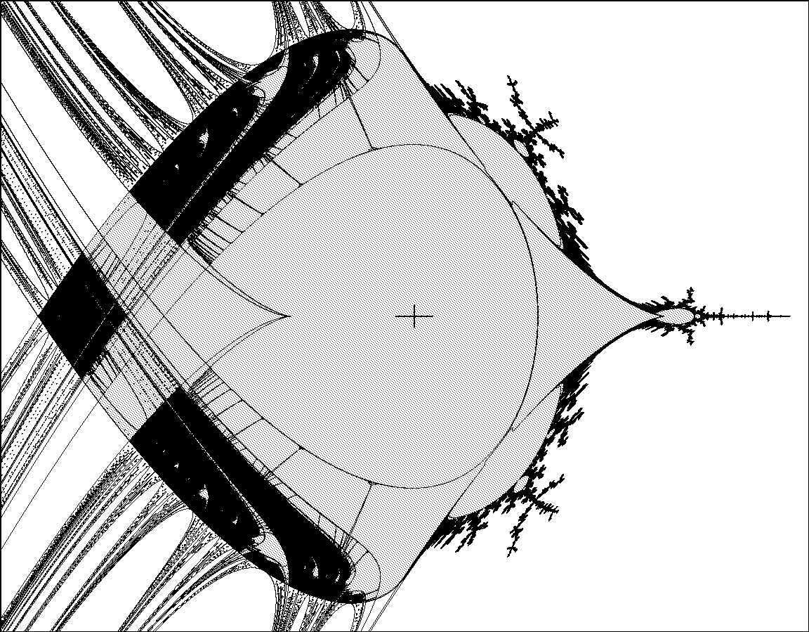
Using the formulation 6.1,we note that ˆG(2) is the direct sum of two cyclic groups of order two, and it follows easily that there are twosuitable antiholomorphic involutions, namely the standard involution γ0 : z 7→¯z and the exotic involutionγ1:z7→−¯z .Thus we consider the two spaces P2R(γj) consisting of monic centered cubic maps satisfying f(z) =(−1)jf(¯z) , for j = 0, 1 . Using the formulation 6.2, we consider instead the two spaces P2±Rconsist-ing of centered cubic maps with real coefficients, and with leading coefficient ±1 .

(Compare Figure 3. )There is a completely analogous discussion for any even w ≥2 .

The space P(w) of polynomials ofdegree w + 1 has exactly two real forms, up to isomorphism. In factˆG(w) is a dihedral group of order2w with two distinct conjugacy classes of anti-holomorphic involutions.

It is most convenient to identifythe corresponding real forms with the spaces P(w)+Rand P(w)−R, consisting of real centered polynomialswith leading coefficient +1 or −1 respectively. The associated groups GR((w)±) = ¯GR((w)±) are allcyclic of order two, generated by the symmetry f(z) 7→−f(−z) .

This symmetry is visible as the reflection(A, b) 7→(A, −b) in Figure 3. On the other hand, if w is odd, then the dihedral groupˆG(w) has just oneconjugacy class of antiholomorphic involutions.

Hence there is a unique real form, consisting of real moniccentered polynomials. In this case, the symmetry group GR((w)+) is trivial.For each reduced mapping schema S of weight two we can make a corresponding computation.

In eachcase it turns out that there are exactly two real forms, which it will be convenient to denote by S+ andS−. (Compare Figures 3-5.) Here S+ corresponds to the space made up out of monic real maps.

For S−,we need different descriptions in the various cases, as follows:For S−= (1, 1)−and S−= (1) + (1)−we must consider monic centered maps from |S| × C to itselfwhich commute with the antiholomorphic involution (v , z) 7→(3 −v , ¯z) . Such maps have the form(v1 , z) 7→(v2 , z2 + c) ,(v2 , z) 7→(v1 , z2 + ¯c)forS = (1, 1)(v1 , z) 7→(v1 , z2 + c) ,(v2 , z) 7→(v2 , z2 + ¯c)forS = (1) + (1) .The corresponding connectedness loci are shown in Figure 4.

In the first case this locus, known as the“tricorn”, has a symmetry group GR((1, 1)−) ∼= G(1, 1) which is non-abelian of order 6, as is visible in theFigure. (Compare [Wi].) For S−= (1) + (1)−, the associated connectedness locus is just a copy of theMandelbrot set, with the involution c 7→¯c as unique real automorphism.For S = ({1}1) , the situation is more confusing, since the connectedness loci for the two real forms({1}1)± are indistinguishable from each other.

We must consider real maps of the form(v1 , x) 7→(v1 , x2 + r1) ,(v2 , x) 7→(v1 , ±x2 + r2) ,22

e in pixelse in pixelsFigure 3. The spaces P(2)+Rand P(2)−Rof real cubic maps, intersected with thecomplex connectedness locus C(2) .These pictures show the (A, b)-plane wherex 7→±x3 −3Ax + b .

(Compare [M3]. )23

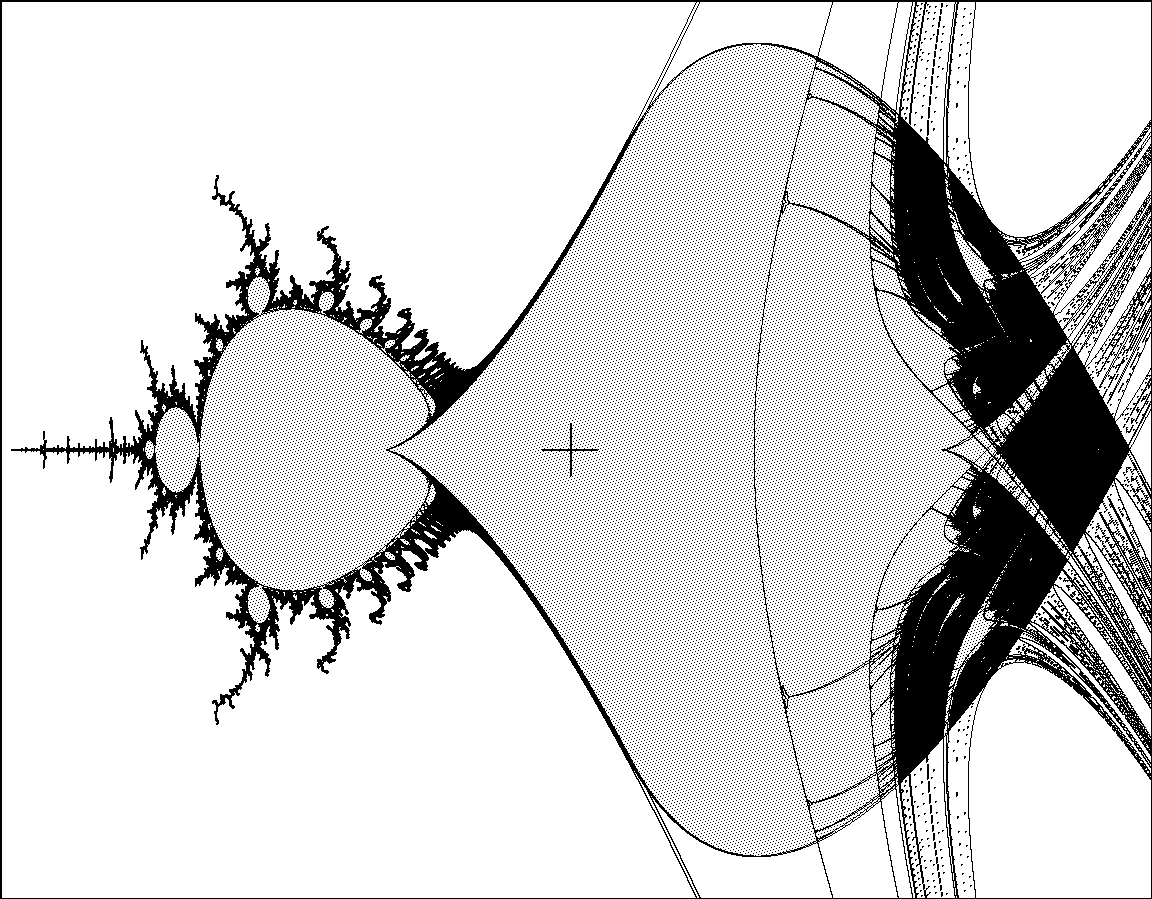
(1, 1)+(1, 1)−(1) + (1) +(1) + (1) −Figure 4. Connectedness loci for four real forms of weight two.wherethechoiceofsignhasverylittleeffectonthedynamics.Inthiscasethegroup¯GR(({1}1)±) of dynamic automorphisms is trivial, even though there is an evident set theoretic auto-morphism (r1 , r2) 7→(r1 , −r2) of the connectedness locus.Remark 6.3.

In analogy with 2.9, there is a partial ordering(2)±≻(1, 1)−≻(1) + (1)−(1, 1)+≻((1) + (1)+({1}1)±for the collection of real forms of total weight two.Our main result in the real case can be stated as follows.Theorem 6.4. Every hyperbolic component in a real connectedness locus of weight w is a topo-logical w-cell with a unique “center” point, and is real analytically homeomorphic to a uniquelydefined principal hyperbolic component HS0R(γ) , or to a suitably defined space BR(S, γ) ofBlaschke products, under a homeomorphism which is uniquely determined up to the action ofthe symmetry group¯GR(S, γ) .The proof involves going through the arguments in previous sections, keeping track of the extra involution,and is not difficult.⊔⊓24

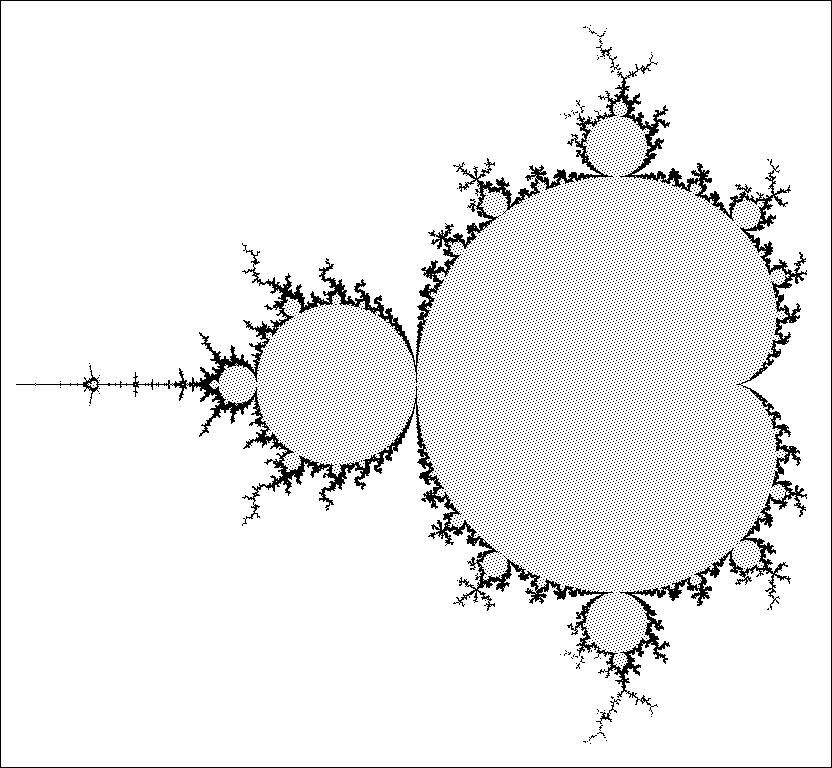
e in pixels({1}1)±Figure 5. Connectedness loci for the remaining two real forms of weight two.§7.

Polynomials with marked critical points.By a critically marked polynomial map of degree w + 1 we will mean a polynomial map f togetherwith an ordered list (c1 , . .

. , cw) of its critical points.

Even if fis a real polynomial, this list mustinclude all complex critical points, so that the derivative f ′(z) is a constant multiple of (z−c1) · · · (z−cw) .Similarly, we can define the concept of a “critically marked” Blaschke product.Branner and Hubbard have shown the utility of studying critically marked polynomial mappings. Allof the principal results of the previous sections extend to the marked case.

For any mapping schema S wecan define a space P♯(S) of marked polynomial maps and a space B♯(S) made up out of marked Blaschkeproducts. Then any hyperbolic component of type S in any marked connectedness locus C♯(S′) ⊂P♯(S′)is canonically homeomorphic to B♯(S) .

The one step in this program which cause additional difficulty isthe analogue of Lemma 3.5, showing that B♯(S) is a topological cell. However, Douady has supplied theauthor with a proof of the following key result.Lemma 7.1.

The space consisting of all critically marked Blaschke products of degree w + 1which fix the points 0 and 1 is a topological cell of dimension 2w .Proof.We will make use of the standard diffeomorphism h : D →C , given by h(z) = w =z/p1 −|z|2 , with inverse z = w/p1 + |w|2 . Let β : D →D be a proper holomorphic map fixing 0 and1 , with (not necessarily distinct) critical points c1 , .

. .

, cw . Consider the composition h ◦β : D →C .Pulling back the standard conformal structure of C under this composition, we obtain a new Riemannsurface Dβ , which has underlying space D but is none-the-less conformally isomorphic to C .

In factwe can choose the conformal isomorphism η : C →Dβ so that η(0) = 0 and limt→+∞η(t) = 1 . Thecomposition h ◦β ◦η will then be a polynomial map of the formz 7→h(β(η(z))) = λZ0(w + 1) (z −ˆc1) · · · (z −ˆcw)dzwith leading coefficient λ > 0 , where η(ˆck) = ck .

In fact, after replacing the function η(z) by η(z/λ1/(w+1)) ,we may assume that λ = 1 . Conversely, given such a monic polynomial with marked critical points whichfixes the origin, we can reverse this construction, thus obtaining a corresponding Blaschke product withmarked critical points.

This proves that the required space of Blaschke products is diffeomorphic to thespace of w-tuples (ˆc1 , . .

. , cw) ∈Cw .

⊔⊓Using 3.4, it follows easily that the space of critically centered Blaschke products with marked critical25

points and with β(1) = 1 is also a topological cell. The proof that the model space B♯(S) is a topologicalcell is now straightforward.For the case of marked polynomial maps, we must expect a group of symmetries which is much largerthan G(S) , and many more real forms than in §6.

The basic definitions are as follows. For any mappingschema S , let Π(S) be the cartesian product, over all vertices v , of the symmetric group of permutationsof the numbers {1, 2, .

. .

, w(v)} which are used to index the critical points in Wv . Then the affine spaceP♯(S) of marked centered polynomial maps from |S| × C to itself can be defined as a normal branchedcovering space of PS , with Π(S) acting as the group of deck transformations.Similarly, the spacesC♯(S) ⊃H♯0(S) and B♯(S) are Π(S)-branched coverings of CS ⊃HS0and of B(S) .

The full groupG♯(S) of symmetries of P♯(S) splits as a semidirect product1 →Π(S) →G♯(S) ←→G(S) →1or1 →N(S) × Π(S) →G♯(S) ←→Aut(S) →1 . (Compare §2.8.

)Rather than working out the full details of this, let me simply describe the simplest case S = (w) . Ifa1 , .

. .

, awarearbitrarycomplexnumberswithbarycentera = (a1 + · · · + aw)/w , then it may be convenient to use the notationz 7→f(z) = f(a1 , . .

. , aw ; z)for the unique marked centered monic map of degree d = w + 1 with critical pointsa1 −a , a2 −a , .

. .

, aw −aand with f(0) = a . Here the symmetric group Π(w) of order w!

acts by permuting the aj , and the groupN(w)ofw-throotsofunityηactsbytherulef(z) 7→ηf(z/η) , or equivalentlyf(a1 , . .

. , aw ; z)7→f(ηa1 , .

. .

, ηaw ; z) .The automorphism group Aut(w) is of course trivial, so that the full symmetry group G♯(w) is just thecartesian product N(w) × Π(w) of order w w! .In order to study real forms, we extend G♯(w) by the antiholomorphic involution γ0 , which commuteswith Π(w) , and look for conjugacy classes of antiholomorphic involutions in the resulting groupˆG♯(w) .For d even, it turns out that there are d/2 distinct real forms, corresponding to polynomial maps witheither 1 , 3 , .

. .

, or w real critical points. For d odd, there are d + 1 distinct real forms.

As an example,for d = 3 there are two marked real formsx 7→±(x3 −3a2x)+bwith real critical points (a, −a) and twomarked real formsx 7→±(x3 + 3a2x) + bwith imaginary critical points (ia, −ia) . (Compare [Brannerand Hubbard].) Further details will be left to the reader.26

AppendixRealizing Reduced Schemata.by Alfredo PoirierWe fix a reduced schema ¯S = (| ¯S|, F, w). The main purpose of this appendix is to show that there exista Postcritically Finite Polynomial f of degree d( ¯S) = w( ¯S) + 1, whose associated reduced schema ¯S(f)realizes ¯S :Theorem.

Every reduced schema ¯S = (| ¯S|, F, w) can be realized.We start by constructing a non reduced schema S which has ¯S as associated reduced schema (compareFigures A.1 and A.2). Let V be the set consisting of two copies of | ¯S|.

Thus to any v ∈| ¯S|, we associatev, v′ ∈V . We set wS(v) = w(v), and because we do not want to increase the degree we define wS(v′) = 0.Next, we define the function FS : V →V as follows.

Let FS(v) = v′ and FS(v′) = F(v). We will realizethis mapping schema S = (|S| = V, FS, wS) by constructing an expanding Hubbard tree (for the definitionsand main results in abstract Hubbard Trees we refer to [P1] or [P2]).In other words we have only inserted between every pair of (critical) vertices a third non-critical one.Clearly when restricted to the set | ¯S|, FS satisfies F ◦2S = F .

The next two lemmas follow directly from theabove construction.Lemma 1. The mapping schema S = (|S|, FS, wS) has reduced schema ¯S .Lemma 2.

Let v′ ∈V be a non critical vertex. If FS(ω) = v′ then v = ω.In other words every non critical vertex has exactly one preimage.S:+Figure A.1: A reduced schema.S:+V10U3V20V21Figure A.2: The associated non-reduced mapping schema.29

We begin the proof that the mapping schema S can be realized, with a preliminary construction. LetCi be the cycle vi0 7→v′i0 7→vi1 7→.

. .

vin = vi0 . For this cycle we will construct a (star-shaped) expandingHubbard Tree H(Ci) as follows.

Join the vertices vij and v′ij to a new vertex pi = pCi . We define the anglebetween consecutive edges at pi as 1/2n.

The new vertex pi will be by definition fixed of degree d(pi) = 1.At all other vertices the dynamics and degree is that induced by S (note that by definition d(v) = w(v)+1).As there is only one periodic point which does not belong to a critical cycle, this is trivially an expandingabstract Hubbard tree.Next, from each critical cycle Ci we choose a critical vertex vi = vi0 and form the collection {v1, . .

. , vm};where m ≥1 is the number of components of S .

Let um+1, . .

. , um+r be the critical vertices which do notbelong to critical cycles.

We construct an expanding abstract Hubbard tree which realizes S as follows.Join the vertices vi and uj to a new vertex q, by segments ℓi and ℓj . At q these segments should formangles of non trivial multiples of 1/(r + m).

Next, for every vertex uj , we join uj and u′j by an edge whichforms an angle of 1/d(uj) with ℓj . Also for every cycle Ci we paste the tree H(Ci) at vi forming an angleof 1/d(vi) with ℓi .

Because of lemma 2 this graph is a topological (angled) tree. If we define q as a fixedvertex of degree 1, then with the induced dynamics from S and all H(Ci) this tree is expanding (compareFigure A.3).

Now, as every expanding Hubbard Tree can be realized by a Postcritically Finite polynomial(see [P1] or [P2]), the result follows.H:*****V’10V10U3U’3qP1P2V’21V20V’20V21Figure A.3: An associated abstract Hubbard Tree which realizes this mapping schema.In this figure ∗represents a critical point (∗∗a double critical point). Dots correspondto points in the Julia set, and circles correspond to centers of Fatou components.

Asthere is no edge whose endpoints correspond to Julia set vertices, this tree is (trivially)by definition expanding.30

References. [AB] L. Ahlfors and L. Bers, The Riemann mapping theorem for variable metrics, Annals of Math.

72(1960), 385-404. [Bl] P. Blanchard, Complex analytic dynamics on the Riemann sphere, Bull.

Am. Math.

Soc. 11 (1984),85-141.

[BDK] P. Blanchard, R. Devaney and L. Keen, The dynamics of complex polynomials and automorphismsof the shift, to appear. [Br] B. Branner, The parameter space for cubic polynomials, pp.

169-179 of “Chaotic Dynamics and Frac-tals”, edit. Barnsley and Demko, Acad.

Press 1986. [BD] B. Branner and A. Douady, Surgery on complex polynomials, pp.

11-72 of “Holomorphic Dynamics,Mexico 1986”, ed. Gomez-Mont et al., Lect.

Notes Math. 1345, Springer 1988.

[BH] B. Branner and J. H. Hubbard, The iteration of cubic polynomials, Part 1: The global topology ofparameter space, Acta Math. 160 (1988) 143-206; Part 2: to appear.

[BM] R. Brooks and P. Matelski, The dynamics of 2-generator subgroups of PSL(2, C) , pp.65-71 of“Riemann Surfaces and Related Topics” (Proceedings 1978 Stony Brook Conference), edit.Kra andMaskit, Ann. Math.

Stud. 97 Princeton U.

Press 1981. [D1] A. Douady, Syst´emes dynamiques holomorphes, S´em.

Bourbaki 599, Ast´erisque 105-106 (1983), 39-63. [D2] A. Douady, L’´etude dynamique des polynˆomes quadratiques complexes et ses reinvestissements, Soc.Math.

France, Assembl. Gen. Jan. 1985, 21-42.

[DE] A. Douady and C. Earle, Conformally natural extension of homeomorphisms of the circle, Acta math.157 (1986), 23-48. [DH1] A. Douady and J. H. Hubbard, ´Etude dynamique des polynˆomes complexes I & II, Publ.

Math. Orsay(1984-85).

[DH2] A. Douady and J. H. Hubbard, On the dynamics of polynomial-like mappings, Ann. Sci.

Ec. Norm.Sup.

(Paris) 18 (1985), 287-343. [La] P. Lavaurs, Syst`emes dynamiques holomorphes: explosion de points p´eriodiques paraboliques, Thesis,Univ.

Paris-Sud Orsay 1989.[LV]O. Lehto and K. I. Virtanen, Quasiconformal Mappings in the Plane, Springer 1973.

[Ly1] M. Lyubich, The dynamics of rational transforms: the topological picture, Russian Math. Surveys41:4 (1986), 43-117.

[Ly2] M. Lyubich, Some typical properties of the dynamics of rational maps, Russian Math. Surveys 38(1983) 154-155.

[Ly3] M. Lyubich, An analysis of the stability of the dynamics of rational functions, Funk. Anal.

i. Pril. 421984), 72-91; Selecta Math.

Sovietica 9 (1990) 69-90. [MSS] R. Ma˜n´e, P. Sad and D. Sullivan, On the dynamics of rational maps, Ann.

Sci. ´Ec.

Norm. Sup.Paris, 16 (1983), 193-217.

[McM] C. McMullen, Automorphisms of rational maps, pp. 31-60 of “Holomorphic Functions and ModuliI”, ed.

Drasin, Earle, Gehring, Kra & Marden; MSRI Publ. 10, Springer 1988.

[M1] J. Milnor, Self-similarity and hairiness in the Mandelbrot set, pp. 211-257 of “Computers in Geometryand Topology”, edit.

Tangora, Lect. Notes Pure Appl.

Math. 114, Dekker 1989.

[M2] J. Milnor, Dynamics in one complex variable: Introductory lectures, Stony Brook IMS Preprint 1990/5. [M3] J. Milnor, Remarks on iterated cubic maps, Stony Brook IMS Preprint 1990/6 (to appear in Experi-mental Mathematics).

[M4] J. Milnor, Remarks on quadratic rational maps, in preparation.31

[P1] A. Poirier, On the realization of fixed point portraits, Stony Brook IMS Preprint 1991/20. [P2] A. Poirier, On postcritically finite polynomials, Thesis, Stony Brook, in preparation.

[P3] A. Poirier, Hubbard forests, in preparation. [R1] M. Rees, Components of degree two hyperbolic rational maps, Invent.

Math. 100 1990, 357-382.

[R2] M. Rees,A partial description of parameter space of rational maps of degree two, Part I: preprint,Univ. Liverpool 1990; and Part II: Stony Brook IMS preprints 1991/4.

[Sh1] M. Shishikura, Surgery of complex analytic dynamical systems, pp. 93-105 of “Dynamical Systemsand Nonlinear Oscillations”, ed.

G. Ikegami, World Scient. Series in Dyn.

Sys. 1, Singapore 1986.

[Sh2] M. Shishikura, On the quasiconformal surgery of rational functions, Ann. Sci.

´Ec. Norm.

Sup. Paris,20 (1987) 1-29.

[Su1] D. Sullivan, Conformal dynamical systems, pp. 725-752 of “Geometric Dynamics”, ed.

J. Palis, Lect.Notes Math. 1007, Springer 1983.

[Su2]D.Sullivan,Quasiconformalhomeomorphismsindynamics,topology,andgeometry,preprint 1986. [Su3] D. Sullivan, Quasiconformal homeomorphisms and dynamics, I, Annals of Math.

122 (1985) 401-418;II, Acta Math. 155 (1985) 243-260; III, to appear.

[Su4] D. Sullivan, Expanding endomorphisms in the complex plane, to appear. [Wi] R. Winters, Bifurcations in families of antiholomorphic and biquadratic maps, Thesis, Boston University1990.32

---

출처: arXiv:9202.210 • 원문 보기