Fast localization of anomalous patches in spatial data under dependence

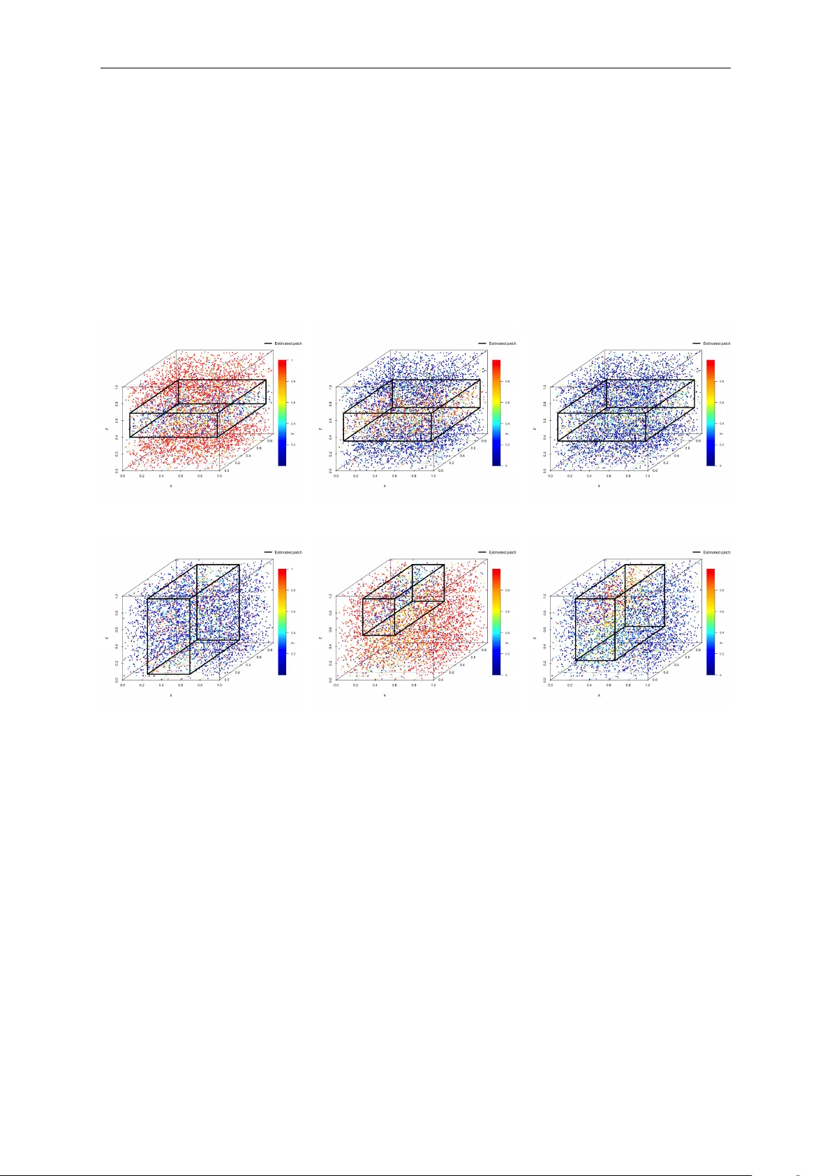
F ast lo calization of anomalous patc hes in spatial data under dep endence Soham Bonnerjee ∗ Sa yar Karmak ar ∗ George Mic hailidis University of Chic ago University of Florida UCLA Abstract W e prop ose a scalable, prov ably accurate metho d for lo calizing an unkno wn num b er of m ultiple axis-aligned anomalous patches in spatial data under a general class of spatial dep endence. Motiv ated b y the practical need to detect localized changes rather than completely segmen t large spatial grids, w e ﬁrst introduce b oth a naiv e and a signiﬁcantly faster in telligent-sampling-based estimator for a single patc h. W e then extend this methodology to the highly challenging m ultiple-patch setting and prop ose a tw o-stage Spatial P atch Lo calization of Anomalies under DEp endence procedure (SPLADE). Under mild conditions on signal strength, separation from the b oundary , in ter-patch separation, and a uniform Gaussian appro ximation, we establish sim ultaneous consistency for the estimated num ber of patches and for eac h individual patch b oundary . Extensiv e numerical results based on synthetic data scenarios demonstrate that the prop osed metho d exhibits signiﬁcant computational and accuracy gains ov er comp eting approaches, as well as robustness to mo derate and severe spatial dep endence. Finally , we demonstrate the real-w orld utilit y of the prop osed method by applying it to frame-to-frame video surveillance data, where it accurately detects small, closely separated sub jects, a task where existing metho ds are signiﬁcan tly slo wer and highly prone to spurious detections due to not accounting for spatial dep endence. A second application on 3D ﬁbrous media is deferred to the App endix. Keywor ds : Spatial dep endence, Anomaly detection, Boundary detection, Multiple change- p oin ts 1 In tro duction Inference for anomalous patches or clusters in spatial data has a long history , going back at least to Besag and Newell [ 1991 ]. The problem is ro oted in the earlier literature on epidemic c hange-p oin ts for time-ordered data [ Levin and Kline , 1985 , Y ao , 1993 , Inclán and Tiao , 1994 , Hušk ov á , 1995 , Csörgő and Horv áth , 1997 , Chen et al. , 2016 , Račk ausk as and Suquet , 2004 , 2006 , Ning et al. , 2012 ], aided b y mathematical tools such as those developed in Naus [ 1965 ]. In the spatial setting, one natural analogue is b oundary or partition reco very , where separating h yp ersurfaces divide the domain in to heterogeneous regions [ Hall et al. , 2001 , Han et al. , 2025 , Song et al. , 2011 , Otto and Schmid , 2016 , F an and Guan , 2018 , Chan et al. , 2022 ]. In man y applications, how ever, the practically relev an t departure is not a global partition, but a lo cal hotsp ot; namely , a small region whose b eha vior diﬀers from its surroundings. This viewp oin t is esp ecially natural in public health [ Hjalmars et al. , 1996 , Souza et al. , 2019 , Lord et al. , 2020 ], public safety and urban planning [ W arden , 2008 , Gao et al. , 2013 , Zeoli et al. , 2014 , Basu Sarbadhik ary et al. , 2025 ], and environmen tal monitoring [ Riitters and Coulston , 2005 , Shac kelford et al. , 2015 , V ega Orozco et al. , 2012 ], where the goal is to screen an en tire map for lo calized excess risk without sp ecifying the anomalous region in adv ance. ∗ Equal contributions 1 2 F ormally , w e mo del the observed data as a d -dimensional lattice ﬁeld X i = µ i + η i , i ∈ [ n ] , (1.1) where n = ( n 1 , . . . , n d ) ∈ N d and [ n ] := Q d ℓ =1 { 1 , 2 , . . . , n ℓ } . Let I := S K j =1 I j denote the union of K (pairwise disjoin t) anomalous patc hes, with each I j ⊆ [ n ] . W e mo del the mean ﬁeld b y a baseline level µ 0 outside the anomalous region and patc h-sp eciﬁc mean shifts inside: µ i = ( µ 0 + δ j , i ∈ I j , j = 1 , . . . , K, µ 0 , i ∈ [ n ] \ I , (1.2) where δ j  = 0 for anomalous patc hes (and δ j 1  = δ j 2 is allo wed). With this formulation, the tw o fundamen tal statistical problems are: (i) to test whether anomalous patc hes exist at all, and (ii) to lo calize them when they do. Lik eliho o d-based spatial scan statistics systematized anomalous patch detection b y computing lik eliho o d ratios ov er candidate regions and using Mon te Carlo calibrations to adjust for multiple testing [ Kulldorﬀ and Nagarwalla , 1995 , Glaz et al. , 2001 ]. Pioneered by Kulldorﬀ [ 1997 ] and p opularized b y the SaTScan soft ware [ Kulldorﬀ , 2006 , Blo c k , 2007 ], this framew ork has b een widely extended. Developmen ts include adaptations for count [ Neill et al. , 2004 , Neill , 2012 ], ordinal [ Jung et al. , 2007 ], and Bernoulli data [ Boutsik as and Koutras , 2006 , W alther , 2010 ], alongside minimax-optimal pro cedures for Gaussian settings [ Arias-Castro et al. , 2005 , 2011 , Chan and W alther , 2013 , Sharpnac k and Arias-Castro , 2016 , Datta and Sen , 2021 , W alther and P erry , 2022 ]. Drawing on limit theory for Gaussian random ﬁelds [ Jiang , 2002 , Kabluc hko , 2011 ], m uch of this literature primarily fo cuses on the testing problem [ W alther , 2010 , W alther and Perry , 2022 , Arias-Castro et al. , 2011 , Sharpnac k and Arias-Castro , 2016 , Gao et al. , 2016 , Arias-Castro et al. , 2018 , Datta and Sen , 2021 , Klein , 2022 , Sto epk er et al. , 2025 , Köhne and Mies , 2025 ], though recent adv ances also include non-parametric, rank-, and p erm utation-based metho ds [ Cucala , 2014 , Jung and Cho , 2015 , Arias-Castro et al. , 2018 , König et al. , 2020 , Sto epk er et al. , 2025 ]. F or comprehensiv e reviews of the extensive scan-statistics literature, see Arias-Castro et al. [ 2011 ], Ab olhassani and Prates [ 2021 ], Xie et al. [ 2022 ]. Conceptually , the “scan statistic” can b e argued to adopt a top-down p erspective: one sp eciﬁes a class of anomalous patterns a priori, and systematically scans the ﬁeld to detect regions consisten t with that structure. On the other hand, there has b een a stream of complementary literature stemming from partition recov ery or anomalous sub-graph or cluster detection problems [ Madrid Padilla et al. , 2021 , Y u et al. , 2022 , W ang and Chao , 2025 ], which usually proceeds via a b ottom-up approach by constructing the anomalous region incrementally from local, ﬁne-scale evidence. In suc h an approach, one can quantify uncertaint y in the b oundary b y constructing lo cation-wise “membership evidence” scores from the ensemble of near-optimal clusters, pro ducing a fuzzy b oundary map rather than a single hard con tour Oliveira and others [ 2018 ]. These distinctions are not mutually exclusive: for example, several subgraph or sub-matrix reco very problems Arias-Castro et al. [ 2011 ], Sharpnack et al. [ 2013 ], Butucea and Ingster [ 2013 ] also p erform scans of some statistics ov er a family of corresp onding candidates, blurring the b oundary b et w een the tw o approac hes. Nevertheless, w e ﬁnd this distinction con venien t for exp osition. Our framew ork aligns closely with the top-down scan-statistic persp ective, though we con textualize this work within b oth frameworks. The c ase for dep endent-data : A v ast ma jorit y of the literature on the “b ottom-up” approac h, p erhaps constrained b y the av ailable theoretical guarantees of the clustering algorithms, exclusiv ely consider indep enden tly distributed observ ations. A similar restriction app ears in a substantial p ortion of the scan-statistics literature as well. This assumption is kno wn to b e consequen tial in practice; for example, Loh and Zh u [ 2007 ] sho w that when spatial data exhibit unmo deled p ositiv e auto correlation, classical scan statistics that assume independence can yield o verly small p -v alues and spurious cluster detections. T o the b est of our knowledge, only a small 3 n umber of w orks consider spatial dep endence in anomalous patc h detection, including Chan et al. [ 2022 ], Dresvyanskiy et al. [ 2020 ], Makogin et al. [ 2024 ], Kirc h et al. [ 2025 ], W ang and Chao [ 2025 ]. Among these, W ang and Chao [ 2025 ] is, to our knowledge, the only w ork that directly addresses the lo calization problem, providing theoretical guarantees for consisten t estimation of both the n umber of anomalous patches and their lo cations; rest of these w orks primarily inv estigate the testing problem for existence of anomalous patc hes. Moreov er, Dresvyanskiy et al. [ 2020 ], Mak ogin et al. [ 2024 ], W ang and Chao [ 2025 ] can be viewed as adopting a b ottom-up p ersp ectiv e, using clustering-based metho ds to construct anomalous regions from lo cal evidence. In con trast, Chan et al. [ 2022 ], Kirc h et al. [ 2025 ] form ulate the problem in the scan-statistics framew ork and concentrate on testing for the presence of anomalous regions. Moreov er, Dresvy anskiy et al. [ 2020 ], Kirc h et al. [ 2025 ] assume M -dep enden t observ ations, which substantially restricts the class of admissible dep endence structures; for example, standard spatial autoregressiv e mo dels [ Anselin and Bera , 1998 , Smirnov and Anselin , 2001 ] generally do not satisfy this assumption. On the other hand, W ang and Chao [ 2025 ] assumes sub-Gaussian tails, which allows the analysis to pro ceed using techniques similar to those dev elop ed for the Gaussian case. This pap er fo cuses on the lo c alization of multiple anomalous p atches under gener al sp atial dep endenc e . Crucially , our metho dology requires only the existence of ﬁnite p -th moments , thereb y seamlessly accommo dating he avy-taile d noise distributions. As noted b y Arias-Castro et al. [ 2011 ], while testing and lo calization may share sup erﬁcial computational traits, they demand fundamentally distinct theoretical assumptions and techniques. By adv ancing the scan- statistics paradigm, we lev erage threshold calibration across spatial scales to establish sharp detection regimes alongside rigorous lo calization guaran tees for structured clusters. Consequently , our metho dology delineates the precise conditions under which anomalous b oundaries can b e reliably lo calized. The c ase for sc alability : Computational feasibilit y is a crucial issue often ov erlo ok ed in the pursuit of optimal detection. F or spatially dep enden t data, W ang and Chao [ 2025 ] prop oses a rank-based scan algorithm (similar to Sharpnack and Arias-Castro [ 2016 ]) that lo calizes arbitrarily shap ed patc hes in approximately O ( | n | 3 / 2 ) time, but lacks accompanying theoretical guarantees. In contrast, the detection algorithms in Chan et al. [ 2022 ] and Kirch et al. [ 2025 ] require O ( | n | 2 ) time. Bottom-up clustering approaches for general anomalous patches t ypically incur ev en higher computational cost, an issue highlighted by Y u et al. [ 2022 ] despite ac hieving optimal statistical rates. While Madrid P adilla et al. [ 2021 ] prescrib es an O ( | n | ) algorithm, our n umerical w ork rev eals its empirical runtime is considerably larger than the metho d prop osed in this pap er. Ultimately , most metho ds for detecting irr e gularly shap e d patc hes [ P atil et al. , 2004 , T ango and T ak ahashi , 2005 , Duczmal et al. , 2007 , T ak ahashi et al. , 2008 , Kim and Jung , 2017 , Otani and T ak ahashi , 2021 , Inoue et al. , 2023 , Oliveira et al. , 2025 ] suﬀer from at least one of four limitations: (i) substantial computational costs, (ii) restrictiv e assumptions on cluster size corresp onding to the anomalous patc h, (iii) reliance on knowing the true num b er of clusters, or (iv) in tractable analyses driv en by indep endence assumptions coupled with machine-learning mo dels that are hard to analyze theoretically . On the other hand, muc h of the scan-statistics literature alleviates computational costs b y restricting the search space to sp eciﬁc geometrical shap es for the anomalies. While the SaTScan soft ware Kulldorﬀ [ 2006 ] fo cuses on circular or elliptical patc hes [ T ango and T ak ahashi , 2005 , Kulldorﬀ et al. , 2006 ], another prominent approac h employs rectangular scan windows. A substan tial b o dy of w ork [ Neill and Mo ore , 2004 , Arias-Castro et al. , 2005 , W alther , 2010 , Arias-Castro et al. , 2011 , Bucchia , 2014 , Sharpnac k and Arias-Castro , 2016 , Bucc hia and W endler , 2017 , K önig et al. , 2020 , Dresvy anskiy et al. , 2020 , K ou , 2023 , Mak ogin et al. , 2024 ] has developed appro ximately linear-time algorithms for detecting axis-parallel (hyper)-rectangular patches in d-dimensional ﬁelds, primarily under indep endence. Theoretically , as noted by Sharpnack and Arias-Castro [ 2016 ], Bucchia and W endler [ 2017 ], scanning o ver rectangular windows facilitates the deriv ation of tight asymptotic results ev en under complex spatial dep endency structures. 4 Moreo ver, rectangular clusters arise naturally in certain applications, including ﬁbrous media [ Wirjadi et al. , 2014 , Dresvyanskiy et al. , 2019 , 2020 ] and data mining [ Huo , 2002 ]. In surv eillance, criminology , and geography , axis-aligned rectangles and related raster-style grids are also preferred for three primary reasons: (i) they are op erationally interpretable, allowing analysts to quic kly link hotsp ots to concrete action levels like street segmen ts [ Chainey et al. , 2008 , Eck et al. , 2005 ]; (ii) regular grids provide comparable micro-units for studying ﬁne-scale heterogeneity , whic h is essen tial since crime is often concen trated at sp eciﬁc micro-places [ Malleson et al. , 2019 , W eisburd , 2015 ]; and (iii) they p ermit fast multiscale scanning and rigorous statistical analysis, even if they are more restrictive than irregular shap es [ W alther , 2010 , Pei et al. , 2009 ]. This utility is also demonstrated in CA VIAR video surv eillance dataset [ Fisher , 2004 , Fisher et al. , 2005 ], where sub jects are iden tiﬁed via rectangular b ounding b oxes. The rectangular represen tation is computationally eﬃcient; as noted in the CA VIAR do cumentation, restricting pro cessing to suc h detection zones signiﬁcantly improv es sp eed while maintaining high p erformance. This shows wh y such b o x-based representations are attractive for surveillance analysis in general. Later, w e analyze a part of the data using our proposed scalable metho d and con trast it with other baselines through the lens of precise lo calization. Main con tributions and P ap er Organization: B y fo cusing on axis-parallel rectangles as a canonical structured class of anomalies, we develop a computationally eﬃcien t O ( | n | ) algorithm that pro vides rigorous detection and lo calization guarantees under signiﬁc antly richer sp atial dep endenc e structur es than previously studied. Our core contributions are organized as follows: • Optimal single-Patch lo c alization (Se ction 2.1 ): W e in tro duce a fast in telligent sub-sampling approac h for lo calizing a single anomalous patc h. Notably , for d = 1 , our method reco vers optimal minimax rates, oﬀering a highly scalable solution for epidemic time-series c hange p oin t lo calization. • Sc alable multi-Patch dete ction (Se ction 3 ): Building on the single-patc h localization algo- rithm, we dev elop a t wo-stage Spatial Patc h Lo calization of Anomalies under DEp endence pro cedure (SPLADE) to simultaneously estimate an unknown numb er of anomalous p atches and their pr e cise b oundaries . SPLADE enjoys strong theoretical guaran tees under mini- mal separation assumptions and is highly scalable, unlik e standard binary segmentation tec hniques that scale p oorly in spatial settings. • Str ong empiric al p erformanc e (Se ction 4 ): Extensive synthetic data experiments illustrate that SPLADE exhibits robustness to tuning parameters. More imp ortan tly , SPLADE enjo ys signiﬁcant gains in sp eed and accuracy across v arious patc h conﬁgurations, signal strength and types of spatial dep endence, compared to existing baselines, including DCAR T [ Madrid P adilla et al. , 2021 ] and recen t extensions DPLS-SAD [ W ang and Chao , 2025 ]. While comp eting metho ds falter under spatial dep endence, our approach consistently ac hieves high Adjusted Rand Indices and lo w normalized Hausdorﬀ distances, all the while main taining attractive computational eﬃciency . • R e al-world eﬃc acy (Se ction 5 and App endix H ): W e v alidate our framework on video surv eillance footage and 3D ﬁbrous media, tw o domains inheren tly characterized b y strong spatial dep endence. F or the ﬁrst application, on video surv eillance, w e demonstrate the abilit y to accurately resolve and bound closely situated sub jects in complex en vironments where baseline methods fail to distinguish individual en tities. In the second application on ﬁbrous media, w e explored b ey ond 2D images to a 3D use-case, underlining the scalability SPLADE enjoys ov er other baselines. All theoretical pro ofs, auxiliary lemmas, and additional simulation studies are deferred to the App endix. Notation: F or i ∈ Z d , | i | = i 1 . . . , i d . Deﬁne a R e ctangle I [ a , b ] ⊆ Z d with end-points a ∈ Z d and b ∈ Z d , given by I [ a , b ] = { x ∈ Z d : a < x ≤ b } , where for tw o v ectors x and y ∈ Z d , we 5 sa y x ≤ y if x j ≤ y j for j = 1(1) d . Note that, | I [ a , b ] | = | b − a | . W e denote I [ 0 , n ] as [ n ] . W e also denote the sample size n := | n | . F or tw o p oin ts a , b ∈ Z d , let | a / b | min := min 1 ≤ k ≤ d | a k /b k | , and corresp ondingly | a / b | ∞ := max 1 ≤ k ≤ d | a k /b k | . F or sequences { a n } and { b n } , a n = O ( b n ) and a n = Θ( b n ) imply lim n →∞ a n /b n < ∞ and lim n →∞ a n /b n → ∞ resp ectiv ely . A ∆ B denotes the symmetric diﬀerence of tw o sets A and B . 2 Lo calization of a single anomalous patc h Next, we introduce a generalized framework for spatial dep endency . This foundation motiv ates our t wo-step lo calization strategy: ﬁrst, a "naive" estimator with established theoretical consistency (Section 2.2 ), and second, an in telligen t-sampling algorithm that ensures computational scalability while main taining theoretical v alidit y (Section 2.3 ). These comp onen ts form the essen tial building blo c ks for our subsequent m ultiple-patch SPLADE methodology . 2.1 Preliminaries: dep enden t spatial ﬁelds Let ( ε i ) i ∈ Z d b e a mean-zero stationary random ﬁeld. W e accommodate a v ery general dep endence structure by assuming only that the ε i ’s satisfy a mild, maximal L p b ound for some p > 2 . F ormally , w e require: Assumption 2.1. F or any r e ctangle I ⊆ [ n ] , deﬁne its p artial sum S ε I := P j ∈ I ε j . Assume that ∥ ε 0 ∥ p < ∞ for some p > 2 . Then, we r e quir e that ∥ max I ⊆ [ n ] | S ε I |∥ p ≤ C ′ | n | 1 / 2 , wher e C ′ is indep endent of n , but may dep end on d and p . Assumption 2.1 serves as a spatial analogue of R osenthal’s or Do ob’s maximal ine quality [ Liu et al. , 2013 , Peligrad et al. , 2007 ]. Proving such inequalities for d ≥ 2 is non-trivial due to lack of total ordering; the independent case was pioneered b y Cairoli [ 1970 ] and extended to sp eciﬁc dep enden t martingales b y others [ Christoﬁdes and Serﬂing , 1990 , Hirsc h , 1995 , W alsh , 2006 ]. Giv en its relativ e obscurity in statistics, w e provide a pro of in App endix § A that also illustrates the mathematical tec hniques central to this pap er. Next, we show v alidit y of Assumption 2.1 across v arious spatial dep endency mec hanisms. Example (m-dependent linear ﬁeld) . Assumption 2.1 easily follows from Cairoli’s inequality for m -dep enden t ﬁelds (See Lemma A.1 ), recen tly studied by Kirc h et al. [ 2025 ]. Example (Linear random ﬁelds) . Assumption 2.1 also holds (Lemma A.2 ) for the broad class of linear random ﬁelds that are not m - dep enden t ε i = X s ∈ Z d a s e i − s , where X s ∈ Z d a s < ∞ , e k i.i.d. with ∥ e 0 ∥ p < ∞ , whic h encompasses the Sp atial Autor e gr essive Mo del (SAR) (See ( 4.1 )) [ Ord , 1975 ] widely used in econometrics and geography [ Anselin and Bera , 1998 , Cressie , 2015 , P aul and Nath , 2024 ]. Later in Section 4 , w e revisit this mo del for sim ulations. Mo ving beyond such sp eciﬁc classes of dep endence, arguably the most general represen tation for ( ε i ) i ∈ Z d is given by the functional form: ε i = g ( e i − s : s ∈ Z d ) , (2.1) where g : N ∞ i =1 R d → R d is a progressiv ely measurable function and the innov ations ( e i ) i ∈ Z d are i.i.d. This represen tation intuitiv ely allows for spatial dep endence from an y direction and 6 is directly inspired from writing the join t distribution of dep endent random v ariables in terms of comp ositions of conditional quantile functions of i.i.d. uniform random v ariables. How ev er, for meaningful analysis, w e m ust control the inﬂuence of distan t indices by imp osing a decay structure on spatial correlations. A standard approac h [ El Mac hkouri et al. , 2013 , Bucchia , 2014 , Steland , 2025 ] is to assume a ﬁnite long-run v ariance. Assumption 2.2. The me an-zer o sp atial r andom ﬁeld ( ε i ) i ∈ Z d has a ﬁnite long-run varianc e σ 2 , deﬁne d by σ 2 = E [ ε 2 0 ] + X i  = 0 E [ ε 0 ε i ] < ∞ A p ertinen t question is whether Assumption 2.2 suﬃces to guaran tee Assumption 2.1 . R emark 2.1 (Assumption 2.1 under general dep endency) . Under mild regularity conditions like Assumption 2.2 , ﬁelds of t yp e ( 2.1 ) satisfy a weak er version of Assumption 2.1 . F or instance, El Machk ouri et al. [ 2013 ] establish: L emma 2.1 (Abridged from Prop osition 1, El Machk ouri et al. [ 2013 ]) . Under Assumption 2.2 , for any r e ctangle I ⊆ [ n ] , ∥ S I ∥ p ≤ C | I | 1 / 2 , wher e C is indep endent of n . Ho wev er, conﬁrming the full maximal inequalit y of Assumption 2.1 under general dep endence remains an op en problem in probability theory , primarily due to the lack of total ordering in Z d . Existing results typically impose a causal structure to leverage Cairoli’s inequality . The most general form ulation currently av ailable (derived from Cuny et al. [ 2025 ] and recorded in Lemma B.1 ) restricts ( 2.1 ) to: ε i = g ( e i − s : s ∈ Z d , s ≥ 0 ) , whic h limits dep endence to sp eciﬁc axial directions. Despite this technical gap for the fully general case, the extensiv e evidence v alidating Assumption 2.1 across diverse settings mak es it a practical and reasonable condition. Under Assumption 2.1 , we next introduce a theoretically v alid but naive estimator for a single anomalous patc h, denoted I 0 . Analyzing its computational limitations naturally motiv ates the fast, scalable algorithm dev elop ed in Section 2.3 . 2.2 A naiv e estimator W e ﬁrst establish k ey notation. Let τ k = ( τ k, 1 , . . . , τ k,d ) ∈ [0 , 1] d for k = 1 , 2 , and denote the true rectangular anomalous patch by I 0 := Q d j =1 [ n j τ 1 ,j , n j τ 2 ,j ] . F or exp ositional simplicity , we assume n j τ k,j ∈ N , ignoring negligible fractional rounding since n − 1 ⌊ nγ ⌋ ∼ γ asymptotically . W e start with the “naive” least-squares estimator as: ˆ I LS ( λ 1 , λ 2 ) = arg min I ⊂ [ n ] nλ 1 < | I | 0 such that max {| a / n | min , 1 − | b / n | max } ≥ c . Generalizing the techniques of Bai [ 1994 ] to spatial random ﬁelds, we establish the consistency of ˆ I LS . Theorem 2.2. Consider the mo del in ( 1.1 ) satisfying Assumption 2.1 for some p > p 2( d − 1) ∨ 2 . L et I 0 satisfy Assumption 2.3 and deﬁne c n = min {| I 0 | /n, 1 − | I 0 | /n } . Pr ovide d nc 2 n δ 2 → ∞ as n → ∞ , the estimator ( 2.2 ) satisﬁes | I 0 ∆ ˆ I LS ( C 0 c n , 1 − C 1 c n ) | = O P ( r − 1 n,δ ) , r n,δ := δ 2 1 − 2( d − 1) /p 2  max { log 2 √ n δ , 1 }  − 2 p 2 / ( d − 1) − 2 , (2.4) for suﬃciently smal l c onstants C 0 , C 1 ∈ (0 , 1) . Theorem 2.2 introduces several imp ortant nuances regarding con vergence rates, suﬃcient conditions, and search space selection. R emark 2.2 (Conv ergence conditions and Assumption 2.3 ) . The suﬃcient condition for conv er- gence is nc 2 n δ 2 → ∞ . When | I 0 | ≍ n , this recov ers the standard optimal condition nδ 2 → ∞ . F or context, W ang and Chao [ 2025 ] ac hieves a lo calization rate of ( max k n k ) δ 2 ≫ log n , which is minimax optimal without the b oundary restrictions of Assumption 2.3 . Comparable rates app ear in Gaussian subgraph detection [ Addario-Berry et al. , 2010 , Y u et al. , 2022 ] and time-series literature, where the minimax b ound nδ 2 ≫ log n relaxes to nδ 2 → ∞ , when change-points are b ounded aw a y from the edges [ W ang et al. , 2020 ]. Crucially , while suc h minimax bounds typically rely on strict (sub-)Gaussian data, our results hold under the signiﬁcantly milder Assumption 2.1 , completely av oiding any reliance on fast tail decay . Of particular interest is the ﬁxed-alternativ e regime ( δ ≍ 1 ), where consisten t lo calization requires c n ≫ n − 1 / 2 . Conv ersely , for degenerate “ﬂat” rectangles (i.e., min k ∈ [ d ] | b k − a k | = 0 ), the patc h v olume satisﬁes | I | ≤ | n | min . Consistency here necessitates a diverging signal δ > n 1 / 2 | n | − 1 min . F or instance, if n = t 0 c for some t 0 ∈ N and c ∈ (0 , 1] d , consistency requires δ → ∞ whenev er d > 2 . Intuitiv ely , the sparse signal from a lo w er-dimensional ﬂat patch is easily o verwhelmed by surrounding baseline noise. More generally , if c n ≍ n − γ , the signal must b e suﬃciently strong suc h that γ < 1 2 + log δ log n . R emark 2.3 (Dualit y of anomalous patc h lo calization) . The rate nc 2 n δ 2 , go verned by c n = min {| I 0 | /n, 1 − | I 0 | /n } , reveals an interesting duality : localization is equally diﬃcult whether the patc h is v anishingly small ( | I 0 | /n → 0 ) or ov erwhelmingly large ( | I 0 | /n → 1 ). While upp er b ounds on patc h size hav e app eared in the literature [e.g., Assumption 2.iii in W ang and Chao , 2025 ], this explicit duality is rarely emphasized, though minimum size constraints o ccasionally app ear W alther [ 2010 ], Sharpnack and Arias-Castro [ 2016 ]. Conceptually , if an anomaly dominates the spatial domain, the baseline eﬀectiv ely corresp onds to the true “anomalous” patc h. R emark 2.4 . (Impact of spatial dimension and conv ergence rates) The rate r n,δ reﬂects an impact of d . F or d = 1 (dep enden t time series), Theorem 2.2 recov ers the standard δ − 2 lo calization rate. See Hušk ová [ 1995 ], Bucchia [ 2014 ] F urther, for a ﬁxed d , if the spatial ﬁeld ( ε i ) i ∈ Z d p ossesses suﬃcien tly many momen ts, such as sub-W eibull tails [ K ontoro vic h , 2014 ], we again reco ver the near-optimal δ − 2 rate, up to logarithmic factors. The primary limitation of ( 2.3 ) is computational: an exhaustive search ov er a grid Q d k =1 { 1 , · · · , n 0 } requires O ( n 2 d 0 ) op erations, whic h is sev erely prohibitive for real-w orld applications. 2.3 In telligen t Sampling for Spatial P atc h Lo calization T o o vercome the O ( n 2 d 0 ) computational b ottlenec k of ˆ I LS , we develop an eﬃcien t sub-sampling algorithm to lo calize I 0 . This metho d will also serv e as a foundational building blo c k for our 8 subsequen t m ulti-patc h algorithm. Building on the “intelligen t sampling” concept in tro duced by Lu et al. [ 2017 ] for univ ariate time series, we substantially generalize the framework to m ulti- dimensional spatial random ﬁelds. The core idea relies on a tw o-stage pro cess: ﬁrst, we apply the naiv e estimator to a coarsely sampled spatial grid to iden tify high-probability candidate regions con taining the patch b oundaries. Second, we restrict the reﬁned searc h space exclusively to these lo calized subsets. This strategy yields massive computational sp eedups without sacriﬁcing statistical accuracy . Figure 1: Illustration of the tw o-stage intelligen t subsampling pro cedure detailed in Algorithm 1 . T o build in tuition b efore formalizing the general algorithm, consider the d = 1 case un- der a ﬁxed-alternativ e regime ( δ ≥ c > 0 ). W e ﬁrst construct a coarse subsample Y = { X 1 , X ⌊ √ n ⌋ , X ⌊ 2 √ n ⌋ , . . . } of size O ( √ n ) . Computing the naiv e estimate ˆ I 1 := ˆ I LS ( Y ) requires only O ( n ) op erations, and by Theorem 2.2 , its endp oin ts are guaran teed to lie within O ( √ n ) of the true anomaly I 0 . Therefore, restricting our second-stage searc h to O ( √ n log n ) neighborho ods around the endp oin ts of ˆ I 1 guaran tees optimal lo calization of I 0 with high probabilit y . This restricted searc h reduces the second-stage complexity to just O ( n log 2 n ) , a stark improv emen t o ver the O ( n 2 ) naive approac h. Generalizing this tw o-stage reﬁnement strategy to d -dimensional ﬁelds yields the prop osed algorithm. Figure 1 provides a schematic illustration of Algorithm 1 . Algorithm 1 Single spatial patc h lo calization 1: Input: X = ( X i ) i ∈ [ n ] , α, κ . 2: for k = 1 to d do 3: L k ← ⌊ n α k ⌋ , M k ← ⌈ n k /L k ⌉ . 4: Y k ← { ( s − 1) L k + 1 : s ∈ [ M k ] } . 5: end for 6: Sub-sampled dataset: Y ← { X i : i ∈ Q d k =1 Y k } , m ← |Y | . 7: ˆ I [ a I ,b I ] ← the preliminary naive estimate based on Y . 8: ˆ L B ← Q d k =1 [ L k a I ,k − C L k n κ k (log n ) 1 /d , L k a I ,k + C L k n κ k (log n ) 1 /d ] . 9: ˆ R B ← Q d k =1 [ L k b I ,k − C L k n κ k (log n ) 1 /d , L k b I ,k + C L k n κ k (log n ) 1 /d ] . 10: ˜ I := arg max i ∈ ˆ L B , j ∈ ˆ R B r | j − i | ( n − | j − i | ) n 2   ¯ X I [ i , j ] − ¯ X I c [ i , j ]   . In particular, the v alidit y and consistency of ˜ I based on Algorithm 1 dep end hea vily on the coarseness of the initial grid. Intuitiv ely , a coarser subsample degrades the ﬁrst-stage estimate, increasing the risk that the local enlargemen t sets ˆ L B and ˆ R B fail to capture the true rectangle’s endp oints. Conv ersely , the initial grid size directly dictates the computational sp eedup of Algorithm 1 ov er ˆ I LS , introducing a fundamental computational-statistical trade-oﬀ. W e formalize this trade-oﬀ in the remarks following our next result, which establishes the consistency 9 of Algorithm 1 . Theorem 2.3. Consider the mo del in ( 1.1 ) . L et n b e suﬃciently lar ge such that r n,δ ≥ ( min k n k ) − κ for some κ > 0 , and assume n 1 − α c 2 n δ 2 → ∞ as n → ∞ . L et ˜ I b e the output of A lgorithm 1 with p ar ameters α, κ > 0 satisfying α + κ < 1 . Under the assumptions of The or em 2.2 , it holds that | ˜ I ∆ I 0 | = O P ( r − 1 n,δ ) . (2.5) The parameter α in Theorem 2.3 go verns a crucial statistical-computational tradeoﬀ. While a smaller α relaxes the suﬃcien t conditions for statistical consistency , a larger α reduces the computational cost of the preliminary estimate ˆ I [ a I ,b I ] at the exp ense of a more costly second-stage reﬁnemen t for ˜ I . W e formalize this tradeoﬀ b elo w. R emark 2.5 (Optimal choice of α ) . F or simplicity , assume p ≫ √ d (so r n,δ ≍ δ 2 up to logarithmic factors) and uniform dimensions n 1 ≍ . . . ≍ n d . Algorithm 1 ’s computational complexity is O ( n 2(1 − α ) + n 2( α + κ ) log 2 n ) . If the patc h size scales as c n ≍ n − γ for some γ ∈ (0 , 1) , consistency requires α ∈ (0 , 1 − 2 γ + 2 log δ log n ) . Balancing computational eﬃciency with this statistical constrain t yields the optimal choice α ⋆ : α ⋆ = ( 1 − κ 2 , γ ∈  0 , 1+ κ 4 + log δ log n  , 1 − 2 γ + 2 log δ log n , γ ∈  1+ κ 4 + log δ log n , 1 2 + log δ log n  . Since δ 2 ≳ n − κ/d , it follo ws that 1+ κ 4 + log δ log n ≥ 1 4 + κ ( 1 4 − 1 2 d ) . W e detail the following obser- v ations for regimes where the patch size is suﬃcien tly large ( γ ∈ (0 , 1 / 4) ). Note that this still accommo dates v anishing patc hes ( c n → 0 when γ > 0 ), provided they do not v anish to o rapidly . • F or d = 2 , arguably the most common practical setting, we hav e α ⋆ = 1 − κ 2 for all γ ∈ (0 , 1 / 4) , pro vided δ 2 ≳ n − κ/ 2 for κ > 0 . Consequently , Algorithm 1 ac hieves a computational complexity of O ( n 1+ κ ) . This represents a massiv e sp eed-up o ver the naiv e estimator ˆ I LS , while preserving the optimal statistical consistency rate for realistically sized anomalous patc hes. • As exp ected, computational complexit y naturally increases as the signal strength δ decreases (whic h corresp onds to a larger κ ). • Under a ﬁxed alternativ e ( δ ≍ 1 ), w e set κ ≈ 0 , making the ideal ﬁrst-stage blo c k length L k ( I ) ≈ √ n k . In this regime, Algorithm 1 achiev es a near-linear run time of O ( n ) up to logarith- mic factors. In contrast, under similar settings, existing approac hes [e.g., W ang and Chao , 2025 ] require O ( n 3 / 2 ) op erations for d = 2 , often without explicit theoretical guarantees for consistency . In summary , while Algorithm 1 successfully leverages subsampling to yield a computationally eﬃcien t and pro v ably v alid estimator, its curren t form ulation fundamen tally assumes the presence of only a single anomalous patch. Since the true n umber of anomalies is rarely kno wn a priori in practice, this framework must b e extended. Building on the foundations established in Section 2.3 , the subsequent section develops a generalized algorithm capable of lo calizing multiple spatial patc hes. 3 Multiple spatial patc h lo calization Next, we address the generalized multi-patc h lo calization problem in tro duced in ( 1.2 ) . T o leverage the computational and statistical eﬃciency of Algorithm 1 , w e decompose the m ultiple-patch problem into several disjoint single-patch lo calization tasks that can b e solved in parallel. This decomp osition relies on a preliminary blo ck-based testing pro cedure. Despite complex spatial dep endence, functional cen tral limit theorems t ypically yield an asymptotic Gaussian structure for the random ﬁeld. Assuming for simplicit y that the long-run v ariance is known , we derive an asymptotic threshold for a coarse screening step. This screening isolates a set of disjoin t candidate regions, eac h containing a single true anomalous patch. W e can then apply Algorithm 10 Figure 2: Illustration of the workings of Algorithm 2 . 1 piecemeal to eac h candidate region. W e in tro duce our prop osed metho d, for multiple patc h detection, as Spatial P atc h Localization of Anomalies under DEp endence (SPLADE), detailing its practical nuances and formal theoretical guarantees b elo w. Figure 2 pro vides a schematic of Algorithm 2 . Assuming the true anomalous patches are suﬃcien tly large and wel l-sep ar ate d (for instance, ov erlapping along the y-axis but separated along the x-axis as in Figure 2 , formalized later in Assumption 3.1 ) the key steps of Algorithm 2 pro ceed as follo ws: • Let µ 0 denote the baseline mean outside the anomalies. The algorithm b egins with a blo c k- based testing strategy using a threshold Q . The sample space [ n ] is partitioned in to n 1 − α equal-sized rectangles, and a simultaneous test of E [ X i ] = µ 0 is p erformed on eac h blo c k. Since the patches are large relative to the blo c k size, uniform Gaussian appro ximations (formalized in Assumption 3.2 ) ensure that all blo c ks substantially ov erlapping with an anomaly are ﬂagged with probabilit y approaching one. • Because the threshold con trols a pre-sp eciﬁed T yp e I error, isolated false p ositiv e blo cks will naturally o ccur. Ho wev er, the probability of these false p ositiv es forming large connected comp onen ts v anishes as n increases. Thus, we isolate only connected regions of blo c ks, denoted C j , that con tain a suﬃcien t n umber of samples. Giv en the separation assumption, eac h selected region C j captures exactly one anomalous patc h, sim ultaneously yielding an accurate estimate of the total n umber of anomalies. • Eac h connected region C j is then en v elop ed by a slightly larger rectangle D j suc h that all D j remain disjoint. Since each D j isolates a single true anomaly , w e can deploy Algorithm 1 in parallel across all D j to accurately lo calize the patches. R emark 3.1 (Computational complexit y of Algorithm 2 ) . As in Remark 2.5 , assume uniform dimensions n 1 ≍ . . . ≍ n d ≍ n 1 /d . The ﬁrst-stage testing requires O ( n ) computations, and the connected comp onents can be iden tiﬁed in O ( | M | ) time using standard graph trav ersal techniques [e.g., Cormen et al. , 2022 ]. Supp ose the mean-shift δ j of each patc h I j satisﬁes δ 2 j ≫ n − κ j /d . Applying Algorithm 1 with parameters ( α j , κ j ) indep enden tly to eac h en veloping region D j yields 11 a computational complexity of O  K X j =1 | I j | 2(1 − α j ) + | I j | 2( α j + κ j ) log 2 n  . Cho osing the optimal α ⋆ j = 1 − κ j 2 in accordance with Remark 2.5 reduces the total complexity to O ( n + P K j =1 | I j | 1+ κ j ) . If the num ber of anomalous patches K = O (1) , applying the trivial b ound max j | I j | ≤ n simpliﬁes this to O ( n 1+max j κ j ) . Algorithm 2 SPLADE: Spatial P atch Lo calization of Anomalies under DEp endence 1: Input: X = ( X i ) i ∈ [ n ] , blo c k length parameter α , ﬁrst-stage threshold Q . 2: for k = 1 to d do 3: L k ← ⌊ n α k ⌋ , M k ← ⌈ n k /L k ⌉ . 4: F or s ∈ [ M k ] , set 5: I k ( s ) :=  ( s − 1) L k + 1 , ( s − 1) L k + 2 , . . . , min { sL k , n k }  . 6: end for 7: F orm blo c ks B s := N d k =1 I k ( s k ) for s = ( s 1 , . . . , s d ) ∈ N d k =1 [ M k ] . 8: Set | B s | = Q d k =1  min { s k L k , n k } − ( s k − 1) L k  . 9: Deﬁne blo c k means X s := 1 | B s | P i ∈ B s X i , s ∈ N d k =1 [ M k ] . 10: Initialize ˜ M . 11: for each s ∈ N d k =1 [ M k ] do 12: if | ¯ X s | > Q then 13: ˜ M ← B s . 14: end if 15: end for 16: Let { C 1 , . . . , C ˆ K } b e the connected comp onen ts of ˜ M , with min j | C j | > n α log n . 17: for j = 1 to ˆ K do 18: for k = 1 to d do 19: ℓ j k ← min s ∈ C j s k ; r j k ← max s ∈ C j s k . 20: end for 21: l j ← [ L 1 ℓ j 1 − cL 1 log n, . . . , L d ℓ j d − cL d log n ] , r j ← [ L 1 r j 1 + cL 1 log n, . . . , L d r j d + cL d log n ] . 22: D j ← I [ l j , r j ] , d j ← | D j | . 23: ˆ I j ← Algorithm 1 ( X i ; i ∈ D j ) . 24: end for 25: return n um b er of patches ˆ K ; estimated patches ˆ I j , j ∈ [ ˆ K ] . Crucially , for ﬁxed alternativ es where all δ j ≍ 1 (implying κ j = 0 ), the o verall runtime is strictly O ( n ) . T o the b est of our kno wledge, this is the only algorithm that achieves line ar-time c omputation for the spatial anomaly lo calization problem. In contrast, existing approaches suc h as W ang and Chao [ 2025 ] require O ( n 3 / 2 ) op erations ev en when K is b ounded by a constan t. As an ticipated in our informal discussion, the v alidity of Algorithm 2 hinges on tw o key condi- tions: (i) the anomalous patches must b e well-separated, and (ii) a suﬃciently sharp Gaussian appro ximation must hold to enable sim ultaneous testing of the ﬁrst-stage blo c k means. W e formalize these assumptions b elow. Assumption 3.1 (Minimum separation) . F or any two r e ctangles I [ i 1 , i 2 ] and I [ j 1 , j 2 ] in [ n ] , deﬁne the pseudo-metric ρ ( I [ i 1 , i 2 ] , I [ j 1 , j 2 ] ) = max k ∈ [ d ] max { 0 , j 1 ,k − i 2 ,k , i 1 ,k − j 2 ,k } , 12 and let ν ( I [ i 1 , i 2 ] , I [ j 1 , j 2 ] ) denote the c orr esp onding maximizer over k ∈ [ d ] . Ther e exists an α ∈ (0 , 1) such that the K disjoint anomalous p atches I 1 , . . . , I K satisfy min j  = k ρ ( I j , I k ) ≥ c 0 n α ν ⋆ j k log n, wher e ν ⋆ j k = ν ( I j , I k ) and I j = Q d k =1 [ n k τ j 1 ,k , n k τ j 2 ,k ] . Assumption 3.1 ensures that any pair of anomalous patches is suﬃcien tly separated along at least one of the d co ordinate axes. The separation parameter α strictly go verns the ﬁrst-stage blo c k-based testing pro cedure in Algorithm 2 . Speciﬁcally , if we partition the domain into rectangular blo c ks with side lengths n α k for k ∈ [ d ] , Assumption 3.1 guarantees that an y tw o distinct patches I j and I k are separated by at least Θ( log n ) many blo cks along their axis of maximal separation, ν ⋆ j k . Assumption 3.2 (Uniform Gaussian approximation) . L et A b e the c ol le ction of r e ctangles in [0 , 1] d . F or some n 0 ∈ N , deﬁne A n 0 ( A ) := P i ∈{ 1 ,...,n 0 } d n 0 A ∩ I [ i − 1 , i ] . In a p ossibly enriche d pr ob ability sp ac e, ther e exists a standar d Br ownian she et W on [0 , 1] d such that sup A ∈A   S n ( A n 0 ( A )) − σ n d/ 2 0 W ( A )   = o P ( n d/q 0 ) , (3.1) for some q > 2 , wher e σ > 0 is deﬁne d as in Assumption 2.2 , and S n ( A n 0 ( A )) = P i ∈ A n 0 ( A ) ε i . Assumption 3.2 plays a cen tral role in our subsequent analysis b y enabling a sim ultaneously v alid, blo ck-based testing pro cedure. Next, we discuss its implications. R emark 3.2 (Discussion on Assumption 3.2 ) . Assumption 3.2 functions as a strengthened we ak invarianc e principle (or functional central limit theorem) for spatial random ﬁelds. The q = 2 case in ( 3.1 ) is well-established for a broad class of stationary spatial random ﬁelds satisfying ( 2.1 ) [ El Machk ouri et al. , 2013 , Bucc hia , 2014 ], building upon a ric h history of classical results [ Wic hura , 1969 , Poghosy an and Rœlly , 1998 , Bulinski and Shashkin , 2007 ]. Stronger uniform Gaussian approximations requiring q > 2 hav e b een extensiv ely dev elop ed primarily for the d = 1 (time series) setting. Beginning with the seminal work of K omios et al. [ 1975 ], a large b o dy of literature has established optimal exp onen ts q = p (with p deﬁned in Assumption 2.1 ) for general stationary time series [ Sakhanenk o , 1984 , 1989 , Zaitsev , 1998 , Sakhanenko , 2006 , Götze and Zaitsev , 2009 , Liu and Lin , 2009 , W u and Zhou , 2011 , Berkes et al. , 2014 , Karmak ar and W u , 2020 , Bonnerjee et al. , 2024 ]. Giv en this substan tial evidence in one dimension, w e adopt Assumption 3.2 as a standing condition for spatial ﬁelds ( d > 1 ). W e do not strictly require the optimal exp onen t q = p , although such rates may w ell b e attainable in higher dimensions. Rigorously establishing these uniform appro ximations for d > 1 remains a highly non-trivial open problem in probability theory , though recent adv ances in multiscale and high-dimensional spatial approximations [e.g., Proksch et al. , 2018 , Kurisu et al. , 2024 ] oﬀer promising steps tow ards this direction. The next result establishes the theoretical consistency guarantees of Algorithm 2 . Theorem 3.1. Supp ose Assumptions 2.1 , 2.2 , and 3.2 hold for the underlying sp atial r andom ﬁeld ( ε i ) i ∈ Z d . F urther, assume the b aseline me an is µ 0 = 0 . R e c al l the deﬁnition of blo cks B s in A lgorithm 2 . L et Q b e the (1 − κ ) -th quantile of max s ∈ Q d k =1 [ M k ( I )] | B s | − 1   σ W ( B s )   for some κ ∈ (0 , 1) . Consider the mo del ( 1.1 ) with a b ounde d numb er of anomalous p atches K ≤ C for some c onstant C > 0 , and let these p atches { I j } j ∈ [ K ] satisfy Assumption 2.3 . • (First stage guar ante e) Assume that the p ar ameter α ∈ (0 , 1) in the ﬁrst stage of A lgorithm 2 is smal l enough to satisfy Assumption 3.1 and min j ∈ [ K ] min k ∈ [ d ] n 1 − α k | τ j 2 ,k − τ j 1 ,k | = Θ(log 1 /d n ) , (3.2) 13 yet lar ge enough to satisfy min  n α log n min j ∈ [ K ] δ 2 j , n α/ 2 p log n | n | − d/q ∞  → ∞ as n → ∞ , (3.3) wher e q > 2 is as deﬁne d in Assumption 3.2 . Then, for Algorithm 2 , it holds that P ( ˆ K = K ) → 1 as n → ∞ . (3.4) • (Se c ond stage guar ante e) F or e ach j ∈ [ K ] , supp ose ther e exists κ j > 0 such that r | I j | ,δ j ≫ ( min k ∈ [ d ] | I j | k ) − κ j . Mor e over, supp ose e ach individual applic ation of A lgorithm 1 within A lgorithm 2 is p erforme d with p ar ameters α j smal l enough such that α j + κ j < 1 , and min j ∈ [ K ] n 2 α log 3 d n | I j | 1+ α j δ 2 j → ∞ . (3.5) Then, for any η > 0 , ther e exists an M η > 0 such that the estimates ˆ K and ˆ I j (for j ∈ [ ˆ K ] ) fr om Algorithm 2 satisfy P  | I j ∆ ˆ I j | > M η r − 1 n,δ j for al l j ∈ [ K ]   ˆ K = K  < η . (3.6) Theorem 3.1 ensures that Algorithm 2 accurately estimates the true num b er of anomalous patc hes while localizing each individual patc h at the optimal rate r n,δ j , matc hing the performance of the naiv e estimator. T o the b est of our knowledge, this establishes Algorithm 2 as the only metho d c ap able of c onsistently lo c alizing r e ctangular anomalies under sp atial dep endenc e, while p otential ly achieving an O ( n ) c omputational c omplexity . The theoretical guaran tees of Theorem 3.1 rely on sp eciﬁc tec hnical conditions gov erning the c hoice of α in the ﬁrst stage and the parameters { α j , κ j } K j =1 in the second stage. W e detail these requiremen ts b elo w. Throughout this discussion, we treat the true num b er of anomalies K as ﬁxed relative to n and n , and we condition on the even t that ˆ K = K . R emark 3.3 (Choice of ﬁrst-stage blo c k-size parameter α ) . The c hoice of α is closely tied to the true patch sizes | I j | and their mean-shifts δ j . F ollowing Remark 2.5 , assume uniform dimensions n 1 ≍ . . . ≍ n d ≍ n 1 /d , and supp ose the relativ e b oundaries τ j 1 ,k , τ j 2 ,k are indep enden t of n . Under these conditions, Assumption 3.1 and ( 3.2 ) are trivially satisﬁed for any α ∈ (0 , 1) , and ( 3.3 ) simpliﬁes to α ∈  max  2 q , − 2 min j ∈ [ K ] log | δ j | log n  , 1  . (3.7) Equation ( 3.7 ) requires q > 2 (from Assumption 3.2 ) and min j ∈ [ K ] | δ j | ≫ n − 1 / 2 . This is an extremely mild low er b ound, ensuring the anomalous patc hes remain discernible at the scale of the lattice Z d . As we detail next, this choice of α also fundamen tally constrains the individual patc h lo calizations in the second stage of Algorithm 2 . R emark 3.4 (Choice of second-stage tuning parameters α j ) . Analyzing ( 3.5 ) under the conditions of Remark 3.3 , the parameters α and α j m ust satisfy n 2 α − 1 − α j δ 2 j → ∞ . This condition is strictly stronger than the nδ 2 → ∞ requiremen t in Theorem 2.2 , reﬂecting the fundamen tal trade-oﬀ necessary to achiev e computational eﬃciency . Ignoring logarithmic factors, this requires α j ∈  0 , 2  α + log | δ j | log n  − 1  , whic h implicitly necessitates α > 1 / 2 − ( log | δ j | ) / log n . Our empirical ablation studies, presented in § 4.1 , highlight the robustness of SPLADE across diﬀerent c hoices of α for v arious ligh t-tailed 14 settings, provided the theoretical constrain ts are satisﬁed. T o further align with Theorem 2.3 , as- sume | δ j | ≍ n − κ j / (2 d ) for κ j ∈ (0 , 2 d ) , and let min j ∈ [ K ] κ j = 0 (meaning at least one patch exhibits a constant-order mean shift). F or suﬃciently large n , we ha ve 1 /q ≫ max j ∈ [ K ] κ j / (2 d log n ) , whic h simpliﬁes the feasible parameter range to: α ∈ (2 /q , 1) and α j ∈  0 , 2  α − κ j 2 d − 1 2  . (3.8) While the O ( n ) complexit y of the ﬁrst stage is independent of α , the eﬃciency of the second stage relies heavily on α j . Ha ving argued κ j ≈ 0 in § 2.3 , in light of ( 3.8 ) w e c ho ose α j = 1 / 2 , whic h yields a fully linear-time algorithm. The discussion on estimating the parameters µ 0 and σ is deferred to App endix F . 4 P erformance Ev aluation In this section, w e pro vide empirical evidence corrob orating the established theoretical guarantees. W e ﬁrst provide a sensitivity analysis on the stability of SPLADE across diﬀeren t c hoices of tuning parameters. Subsequen tly , we compare it extensively against three baselines: DCAR T [ Madrid Padilla et al. , 2021 ], a fused-lasso approac h denoted as TV [ T ansey and Scott , 2015 ], and, in selected settings, DPLS-SAD [ W ang and Chao , 2025 ]. An implemen tation of SPLADE is publicly av ailable at https://gith ub.com/soham b01/SPLADE . W e ev aluate computational eﬃciency , lo calization accuracy , and robustness across v arying grid sizes and anomalous patch la youts, spatial dep endence structures, and signal strengths. P erformance is assessed using the follo wing metrics: the mean n umber of detected patc hes, the empirical probability of correctly estimating the true n umber of patches, the Adjusted Rand Index (ARI), the av erage runtime p er iteration (in seconds 1 ), and the normalized Hausdorﬀ distance deﬁned as follows: F or G := { 1 , . . . , N } × { 1 , . . . , N } , Λ 0 := G \ S K k =1 Λ k , b Λ 0 := G \ S b K k =1 b Λ k , let C := { Λ k : 0 ≤ k ≤ K, Λ k  = ∅ } , b C := { b Λ k : 0 ≤ k ≤ b K , b Λ k  = ∅ } . F or A, B ⊆ G , deﬁne the Jaccard distance d J ( A, B ) := | A △ B | / | A ∪ B | with the conv ention d J ( ∅ , ∅ ) = 0 . The normalized t wo-sided Hausdorﬀ distance b et ween C and b C is d H ( C , b C ) := max ( max C ∈C min b C ∈ b C d J ( C, b C ) , max b C ∈ b C min C ∈C d J ( b C , C ) ) . All rep orted results are a veraged ov er 100 indep enden t replicates across div erse exp erimen tal conditions. 4.1 Sensitivit y analysis for SPLADE In this section, we consider the following setting. • Grid sizes ( N × N ): F or ablation, N = 500 , 750 and 1000 . • Conﬁgur ation 1 of anomalous p atches: La y out of 3 true patches (Figure 3a ). • Sp atial dep endenc e structur e: W e consider a SAR( ρ ) process deﬁned as ε i = ρ X j ∈N ( i ) w ij ε j + e i , (4.1) with e i iid ∼ N (0 , 1) and w ij = 1 { j ∈N ( i ) } |N ( i ) | , where neighborho od N ( i ) can hav e cardinality of 2, 3 or 4 dep ending on i -th pixel’s p osition at corner, edge or interior respectively . F or 1 All computations are run on 13th Gen in tel(R) Core(TM) i9-13900K 15 (a) Individual jumps are δ µ (left), δ µ (top right), and − δ µ (b ottom right) (b) Individual jumps are δ µ (b ottom left), 2 δ µ (top left), 3 δ µ (top right), 4 δ µ (b ottom right), and 5 δ µ (cen ter) Figure 3: Illustration of anomalous patch conﬁgurations used for p erformance assessmen t. the sensitivity analysis, w e v ary ρ ∈ { 0 . 25 , 0 . 5 } , and keep the signal strength δ µ in the anomalous patc hes ﬁxed at 1 . Some additional ablation studies for a non-linear distribution are deferred to App endix G.1 . A cross all exp erimen tal settings, w e implemen t SPLADE (Algorithm 2 ) with v arying α ∈ { 0 . 4 , 0 . 5 , 0 . 6 } , and we ﬁx the second-stage tuning parameters (Algorithm 1 ) to α j = 0 . 5 for all j ∈ [ ˆ K ] . The corresp onding results are presented in T able 1 . SPLADE seems to p erform equally well for all three choices of α . This result is not surprising based on ( 3.7 ) and ( 3.8 ) , whose prescrib ed ranges are b eing further widened by the light-tailed Gaussian distribution of the SAR( ρ ) errors. Importantly , our theoretical results require only the minimal assumption of a ﬁnite p -th momen t, and so the theoretically motiv ated c hoices of α ma y , prima facie, seem somewhat conserv ativ e. Nevertheless, SPLADE is robust across a wide range of α , highlighting its stability and further strengthening the consistent improv emen ts in b oth accuracy and sp eed o ver comp etitors in § 4.2 . T able 1: Sensitivity analysis of SPLADE (on α from Stage 1 of Algorithm 2 ) for Conﬁg. 1 with δ µ = 1 under SAR ρ . Each cell reports a verage o ver 100 replicates in the order α = 0 . 4 / α = 0 . 5 / α = 0 . 6 . N SAR( ρ ) ˆ K mean I ( ˆ K = 3) ARI Hausdorﬀ 500 0.25 3.01 / 3.02 / 3.00 0.99 / 0.98 / 1.00 0.986 / 0.975 / 0.977 0.051 / 0.090 / 0.063 0.50 3.01 / 3.02 / 3.00 0.99 / 0.98 / 1.00 0.977 / 0.967 / 0.969 0.078 / 0.111 / 0.085 750 0.25 3.00 / 3.00 / 3.00 1.00 / 1.00 / 1.00 0.982 / 0.985 / 0.983 0.034 / 0.044 / 0.050 0.50 3.00 / 3.00 / 3.00 1.00 / 1.00 / 1.00 0.979 / 0.984 / 0.977 0.049 / 0.048 / 0.065 1000 0.25 3.00 / 3.00 / 2.98 1.00 / 1.00 / 0.96 0.993 / 0.996 / 0.980 0.018 / 0.014 / 0.059 0.50 3.00 / 3.00 / 2.97 1.00 / 1.00 / 0.95 0.991 / 0.991 / 0.976 0.024 / 0.033 / 0.071 4.2 Comparativ e studies In this section, we provide a detailed comparison against other baseline approac hes across diverse settings. In particular, w e consider the follo wing. • Grid sizes ( N × N ): Owing to scalability and other restrictions in the comparative study (eg. the restriction of 2 k × 2 k for DCAR T), we choose N = 256 and 512 . • Conﬁgur ation 2 of anomalous p atches: In addition to Conﬁguration 1 in § 4.1 , we also consider a lay out of 5 true patches (Figure 3b ), closely mirroring Scenario 4 from DCAR T prop osed in Madrid P adilla et al. [ 2021 ]. 16 • Sp atial dep endenc e structur e: Similar to § 4.1 , we consider SAR( ρ ) pro cess with ρ ∈ { 0 . 04 , 0 . 4 , 0 . 8 } . Here, the ρ = 0 . 04 appro ximates the i.i.d. setting assumed by DCAR T. Some additional simulations for a non-linear distribution are deferred to App endix G . • Signal str engths: W e v ary the signal strength δ µ ∈ { 0 . 2 , 0 . 4 , 0 . 6 , 0 . 8 , 1 } for an exhaustiv e picture of the p erformance of SPLADE in b oth lo w and high SNR regimes. F or this section, across all exp erimen tal settings, we implement SPLADE (Algorithm 2 ) with the ﬁrst-stage parameter set to α = 0 . 5 , and we ﬁx the second-stage tuning parameters (Algorithm 1 ) to α j = 0 . 5 for all j ∈ [ ˆ K ] . F or the baseline metho ds, DCAR T and TV, we deﬁne the penalty parameter grids for λ as { 5 , 6 . 78 , . . . , 30 } and { 10 c : c ∈ {− 1 , − 0 . 785 , . . . , 3 }} , resp ectiv ely , follo wing the default recommendations in Madrid Padilla et al. [ 2021 ]. T able 2: Comparison of DCAR T, SPLADE and TV across grid sizes, jump sizes, and SAR ρ for Conﬁg. 1 (Fig 3a ). Each cell reports a verage o ver 100 replicates in the order DCAR T / SPLADE / TV. Jump ˆ K I ( ˆ K = 3) ARI Hausdorﬀ distance time/iter (sec) Grid = 256 × 256 ρ = 0 . 04 0.2 4.78 / 3.66 / 1.34 0.09 / 0.43 / 0.03 0.187 / 0.490 / 0.006 0.86 / 0.86 / 0.96 8.88 / 2.58 / 4.92 0.4 3.72 / 3.00 / 1.18 0.25 / 1.00 / 0.00 0.353 / 0.702 / 0.026 0.93 / 0.52 / 0.95 8.81 / 4.24 / 5.36 0.6 2.83 / 3.00 / 1.31 0.31 / 1.00 / 0.03 0.275 / 0.792 / 0.057 0.95 / 0.38 / 0.95 8.85 / 5.05 / 5.87 0.8 2.63 / 3.00 / 1.42 0.34 / 1.00 / 0.01 0.249 / 0.866 / 0.097 0.96 / 0.25 / 0.96 8.99 / 6.04 / 6.18 1.0 2.99 / 2.99 / 1.38 0.37 / 0.99 / 0.04 0.274 / 0.886 / 0.140 0.97 / 0.20 / 0.95 8.98 / 6.37 / 6.72 ρ = 0 . 40 0.2 7.74 / 1.68 / 1.32 0.04 / 0.12 / 0.04 0.040 / 0.108 / 0.005 0.99 / 0.95 / 0.95 16.38 / 1.21 / 8.85 0.4 7.02 / 3.07 / 1.39 0.09 / 0.93 / 0.05 0.052 / 0.685 / 0.022 0.99 / 0.58 / 0.96 8.93 / 3.77 / 5.60 0.6 6.21 / 3.00 / 1.37 0.07 / 1.00 / 0.04 0.013 / 0.789 / 0.049 1.00 / 0.39 / 0.96 9.00 / 4.89 / 6.07 0.8 5.82 / 3.00 / 1.45 0.09 / 1.00 / 0.03 0.022 / 0.858 / 0.083 1.00 / 0.26 / 0.96 9.03 / 5.56 / 6.33 1.0 5.26 / 3.00 / 1.40 0.14 / 1.00 / 0.05 0.028 / 0.892 / 0.123 1.00 / 0.20 / 0.95 9.12 / 6.04 / 6.83 ρ = 0 . 80 0.2 28.95 / 0.10 / 2.00 0.00 / 0.00 / 0.24 − 0 . 002 / 0.002 / 0.001 1.00 / 0.94 / 0.98 36.00 / 0.14 / 6.09 0.4 28.77 / 0.79 / 2.15 0.00 / 0.04 / 0.31 − 0 . 002 / 0.049 / 0.008 1.00 / 0.94 / 0.98 36.05 / 0.37 / 6.43 0.6 28.51 / 2.92 / 2.00 0.00 / 0.30 / 0.24 − 0 . 002 / 0.289 / 0.019 1.00 / 0.93 / 0.98 36.17 / 1.38 / 6.60 0.8 28.25 / 3.66 / 2.03 0.00 / 0.43 / 0.22 − 0 . 002 / 0.656 / 0.034 1.00 / 0.75 / 0.98 36.20 / 3.17 / 6.82 1.0 28.12 / 3.21 / 2.30 0.00 / 0.80 / 0.28 − 0 . 003 / 0.815 / 0.052 1.00 / 0.43 / 0.99 36.71 / 4.62 / 7.18 Grid = 512 × 512 ρ = 0 . 04 0.2 3.60 / 5.71 / 1.10 0.33 / 0.04 / 0.01 0.348 / 0.369 / 0.003 0.92 / 0.97 / 0.98 68.31 / 9.34 / 31.20 0.4 2.53 / 3.00 / 1.12 0.27 / 1.00 / 0.01 0.203 / 0.782 / 0.010 0.97 / 0.43 / 0.98 40.44 / 20.33 / 22.91 0.6 2.04 / 3.00 / 1.30 0.23 / 1.00 / 0.04 0.211 / 0.891 / 0.022 0.95 / 0.23 / 0.97 40.79 / 26.08 / 25.13 0.8 1.97 / 3.00 / 1.13 0.15 / 1.00 / 0.00 0.200 / 0.948 / 0.037 0.96 / 0.11 / 0.96 65.32 / 43.92 / 37.55 1.0 2.17 / 3.00 / 1.25 0.24 / 1.00 / 0.01 0.306 / 0.967 / 0.054 0.93 / 0.06 / 0.95 37.92 / 27.52 / 23.73 ρ = 0 . 40 0.2 9.57 / 0.06 / 1.25 0.01 / 0.00 / 0.02 0.107 / 0.002 / 0.002 1.00 / 0.94 / 0.98 68.99 / 0.36 / 31.79 0.4 8.40 / 3.23 / 1.28 0.05 / 0.81 / 0.02 0.019 / 0.764 / 0.009 1.00 / 0.53 / 0.98 40.68 / 15.34 / 23.71 0.6 6.99 / 3.00 / 1.24 0.08 / 1.00 / 0.02 0.036 / 0.877 / 0.021 1.00 / 0.28 / 0.97 40.84 / 22.12 / 24.99 0.8 7.12 / 3.00 / 1.26 0.14 / 1.00 / 0.04 0.045 / 0.934 / 0.035 1.00 / 0.15 / 0.96 66.66 / 40.63 / 40.27 1.0 6.36 / 3.00 / 1.32 0.13 / 1.00 / 0.05 0.061 / 0.963 / 0.052 1.00 / 0.07 / 0.95 38.13 / 26.40 / 25.07 ρ = 0 . 80 0.2 104.32 / 0.00 / 1.56 0.00 / 0.00 / 0.04 − 0 . 001 / 0.000 / 0.001 1.00 / 0.94 / 0.98 565.48 / 0.42 / 49.88 0.4 103.90 / 0.00 / 1.52 0.00 / 0.00 / 0.12 − 0 . 001 / 0.000 / 0.005 1.00 / 0.94 / 0.98 425.19 / 0.36 / 48.41 0.6 103.82 / 0.52 / 1.70 0.00 / 0.00 / 0.12 − 0 . 001 / 0.026 / 0.013 1.00 / 0.94 / 0.98 437.93 / 0.71 / 52.72 0.8 103.54 / 4.88 / 1.68 0.00 / 0.18 / 0.14 − 0 . 001 / 0.363 / 0.023 1.00 / 0.96 / 0.98 471.83 / 4.88 / 55.70 1.0 102.66 / 4.44 / 1.66 0.00 / 0.18 / 0.12 − 0 . 001 / 0.901 / 0.035 1.00 / 0.66 / 0.97 409.01 / 13.68 / 56.61 T ables 2 and 3 summarize the comparativ e p erformance of DCAR T, SPLADE, and TV across a diverse range of exp erimen tal conﬁgurations. Notably , DPLS-SAD [ W ang and Chao , 2025 ] is excluded from these comprehensiv e ev aluations due to its prohibitiv e computational run time; in 17 T able 3: Comparison of DCAR T, SPLADE and TV across grid sizes, jump sizes, and SAR ρ for Conﬁg. 2 (5 patches). Each cell reports a verage o ver 100 replicates in the order DCAR T / SPLADE / TV. Jump ˆ K I ( ˆ K = 5) ARI Hausdorﬀ distance time/iter (sec) Grid = 256 × 256 ρ = 0 . 04 0.2 6.30 / 4.78 / 1.33 0.14 / 0.68 / 0.00 0.621 / 0.752 / 0.059 0.84 / 0.75 / 0.97 9.94 / 4.01 / 4.93 0.4 5.72 / 5.00 / 1.54 0.34 / 1.00 / 0.00 0.797 / 0.877 / 0.194 0.89 / 0.40 / 0.98 9.69 / 4.99 / 5.38 0.6 5.52 / 5.00 / 6.00 0.34 / 1.00 / 0.34 0.851 / 0.930 / 0.831 0.73 / 0.21 / 0.99 9.76 / 5.36 / 3.76 0.8 5.86 / 5.00 / 6.72 0.27 / 1.00 / 0.18 0.878 / 0.951 / 0.852 0.73 / 0.13 / 0.99 9.67 / 5.65 / 4.00 1.0 6.16 / 5.00 / 7.32 0.22 / 1.00 / 0.05 0.905 / 0.958 / 0.902 0.74 / 0.10 / 0.99 9.85 / 5.77 / 3.97 ρ = 0 . 40 0.2 9.82 / 4.24 / 1.49 0.04 / 0.24 / 0.00 0.402 / 0.715 / 0.051 1.00 / 0.90 / 0.98 9.62 / 3.57 / 4.92 0.4 8.91 / 5.01 / 1.68 0.04 / 0.95 / 0.01 0.528 / 0.865 / 0.172 1.00 / 0.50 / 0.98 9.79 / 4.85 / 5.47 0.6 9.02 / 5.00 / 2.20 0.05 / 1.00 / 0.02 0.651 / 0.920 / 0.302 0.99 / 0.26 / 0.99 9.80 / 5.28 / 5.72 0.8 9.18 / 5.00 / 7.01 0.02 / 1.00 / 0.10 0.668 / 0.944 / 0.834 1.00 / 0.16 / 0.99 9.71 / 5.57 / 4.07 1.0 9.51 / 5.00 / 7.67 0.01 / 1.00 / 0.04 0.713 / 0.954 / 0.855 1.00 / 0.11 / 0.99 9.95 / 5.72 / 4.00 ρ = 0 . 80 0.2 29.07 / 2.85 / 2.13 0.00 / 0.03 / 0.00 − 0 . 002 / 0.456 / 0.020 1.00 / 0.96 / 0.99 37.35 / 2.23 / 5.34 0.4 28.72 / 4.13 / 2.29 0.00 / 0.18 / 0.01 − 0 . 002 / 0.738 / 0.078 1.00 / 0.92 / 0.99 37.34 / 3.86 / 5.83 0.6 28.79 / 4.43 / 2.89 0.00 / 0.39 / 0.05 − 0 . 001 / 0.818 / 0.147 1.00 / 0.80 / 1.00 37.58 / 4.57 / 6.10 0.8 28.83 / 4.74 / 3.82 0.00 / 0.68 / 0.19 − 0 . 001 / 0.865 / 0.203 1.00 / 0.61 / 1.00 38.00 / 4.96 / 6.40 1.0 29.41 / 4.97 / 5.71 0.00 / 0.89 / 0.20 0.043 / 0.908 / 0.239 1.00 / 0.38 / 1.00 38.60 / 5.28 / 6.37 Grid = 512 × 512 ρ = 0 . 04 0.2 5.86 / 4.89 / 1.22 0.30 / 0.67 / 0.00 0.729 / 0.822 / 0.023 0.82 / 0.78 / 0.97 36.43 / 18.76 / 20.76 0.4 5.91 / 5.00 / 1.27 0.27 / 1.00 / 0.00 0.849 / 0.944 / 0.059 0.79 / 0.27 / 0.97 37.15 / 23.49 / 22.81 0.6 6.03 / 5.00 / 1.39 0.25 / 1.00 / 0.00 0.895 / 0.969 / 0.080 0.78 / 0.14 / 0.97 36.94 / 24.09 / 24.46 0.8 5.86 / 5.00 / 1.40 0.30 / 1.00 / 0.00 0.929 / 0.981 / 0.103 0.59 / 0.07 / 0.97 37.57 / 24.61 / 26.88 1.0 5.87 / 5.00 / 1.43 0.19 / 1.00 / 0.00 0.940 / 0.986 / 0.162 0.47 / 0.04 / 0.97 39.75 / 28.11 / 30.21 ρ = 0 . 40 0.2 11.58 / 4.10 / 1.24 0.05 / 0.10 / 0.00 0.428 / 0.776 / 0.022 1.00 / 0.95 / 0.97 36.81 / 16.70 / 21.00 0.4 10.70 / 5.07 / 1.36 0.03 / 0.94 / 0.00 0.527 / 0.936 / 0.061 1.00 / 0.32 / 0.97 37.37 / 22.87 / 23.54 0.6 9.67 / 5.00 / 1.46 0.03 / 1.00 / 0.00 0.629 / 0.966 / 0.087 0.98 / 0.16 / 0.97 37.15 / 24.02 / 24.92 0.8 9.62 / 5.00 / 1.57 0.02 / 1.00 / 0.00 0.691 / 0.978 / 0.113 0.97 / 0.09 / 0.98 37.74 / 24.64 / 26.92 1.0 9.53 / 5.00 / 1.53 0.00 / 1.00 / 0.00 0.731 / 0.985 / 0.168 1.00 / 0.04 / 0.98 39.96 / 27.99 / 31.05 ρ = 0 . 80 0.2 103.40 / 2.25 / 1.72 0.00 / 0.02 / 0.00 − 0 . 001 / 0.360 / 0.014 1.00 / 0.96 / 0.98 404.87 / 4.33 / 42.81 0.4 102.85 / 3.71 / 1.79 0.00 / 0.04 / 0.00 − 0 . 001 / 0.732 / 0.051 1.00 / 0.95 / 0.98 404.71 / 14.33 / 48.50 0.6 103.18 / 4.04 / 1.92 0.00 / 0.04 / 0.00 − 0 . 001 / 0.845 / 0.095 1.00 / 0.94 / 0.99 419.63 / 20.06 / 53.21 0.8 106.10 / 4.70 / 2.00 0.00 / 0.58 / 0.00 − 0 . 001 / 0.876 / 0.139 1.00 / 0.77 / 0.99 383.13 / 20.81 / 55.35 1.0 112.32 / 5.20 / 2.16 0.00 / 0.82 / 0.00 0.019 / 0.963 / 0.187 1.00 / 0.28 / 0.99 317.32 / 25.55 / 51.02 18 man y of our exp erimental conﬁgurations, the algorithm failed to terminate within a practical time frame. Regarding computational eﬃciency , SPLADE is consistently the fastest metho d across nearly all settings; in the rare instances where TV marginally outp erforms it, TV incurs a sev ere cost in accuracy . While a verage iteration times naturally scale with grid size and spatial dep endence, SPLADE maintains a distinct adv antage in these more challenging scenarios, achieving speed-ups of up to 15–20x ov er DCAR T and 4x o ver TV. F urther, while the 5-patc h lay out (Conﬁguration 2) increases the computational burden for all metho ds, it concurrently highlights the most substan tial relative sp eed impro vemen ts for SPLADE. It is imp ortan t to note that DCAR T w as implemen ted with an Rcpp accelerator, which makes the contrast in sp eed even more stark. In terms of statistical performance, SPLADE generally yields the most accurate estimation of the true num b er of patches, struggling only when the baseline jump size is exceptionally small. Strong spatial dep endence ( ρ = 0 . 8 ) degrades the p erformance of all metho ds; ho wev er, as the jump size (and corresp ondingly , the signal-to-noise ratio) increases, SPLADE recov ers its count accuracy muc h more rapidly than comp eting metho ds. A similar trend is evident in the A djusted Rand Index (ARI). SPLADE comprehensively outp erforms the competing metho ds, and it is the only approac h whose ARI reliably approaches 1 under high dep endence as the signal strength gro ws. Finally , ev aluating lo calization accuracy via the normalized Hausdorﬀ distance reveals that SPLADE’s estimation error decreases signiﬁcan tly as the jump size increases, whereas the error rates of DCAR T and TV stagnate or exhibit only marginal improv emen ts. T able 4 compares DPLS-SAD and SPLADE on a reduced 64 × 64 grid, a necessary constrain t to b ypass the severe computational b ottlenec ks DPLS-SAD encoun ters on larger domains. Because the original co de is una v ailable, w e ev aluated DPLS-SAD using a custom implementation based directly on the authors’ pseudoco de. F or this targeted exp erimen t, we test dep endence levels ρ ∈ { 0 . 2 , 0 . 4 , 0 . 6 } and jump sizes δ µ ∈ { 0 . 5 , 0 . 75 , 1 } . The trends across all accuracy metrics align closely with our broader ﬁndings against DCAR T and TV. Computationally , SPLADE achiev es massiv e sp eedups of 50 to 100 × o ver our pure R implemen tation of DPLS-SAD (noting that, unlik e the pro vided DCAR T pac k age, our DPLS-SAD implemen tation lacks Rcpp acceleration). W e further contextualize this stark diﬀerence in time complexit y in the real data analysis (Section 5 ). 5 Real-w orld data application: video surveillance fo otage In this section, we demonstrate the practical utilit y of our prop osed metho d through the analysis of video surveillance fo otage. Sp eciﬁcally , we apply SPLADE to capture the spatial dynamics of t wo individuals meeting, ev aluating the metho d’s resolution and lo calization accuracy as the sub jects ph ysically approach one another. An additional real-world application concerning anomaly detection in ﬁb er systems is deferred to App endix H . The CA VIAR pro ject 2 serv es as a foundational b enchmark in the ﬁeld of public surv eillance. It pro vides staged indoor video sequences featuring realistic scenarios, frame-level annotations, and seman tically lab eled b eha viors suc h as walking alone, meeting, and windo w shopping. Due to its high-qualit y ground truth, the dataset has been widely adopted for the repro ducible ev aluation of detection, tracking and high-level activity analysis [ Fisher , 2004 , CA VIAR Pro ject , 2005 ]. F urther, it has signiﬁcan tly inﬂuenced the dev elopment of context-a w are p erception for am bient in telligence and h uman-centered video understanding [ Cro wley and Reignier , 2003 ]. Subsequen t research has utilized CA VIAR for diverse tasks, including short-term activity recognition [ Rib eiro and San tos-Victor , 2005 ], anomalous tra jectory detection [ Sillito and Fisher , 2008 ], and multi-target tracking with so cial grouping cues [ Qin and Shelton , 2012 ] and c hange p oin t analysis [ Bai et al. , 2020 ]. It remains a staple b enc hmark in contemporary surv eys of 2 EC F unded CA VIAR pro ject/IST 2001 37540, a v ailable at: http://homepages.inf.ed.ac.uk/rbf/CA VIAR/. 19 T able 4: Comparison of DPLS-SAD and SPLADE across grid sizes, jump sizes, and SAR ρ for Conﬁg. 1 (3 patches). Each cell rep orts a verage o ver 100 replicates in the order DPLS-SAD / SPLADE. Jump ˆ K I ( ˆ K = 3) ARI Hausdorﬀ distance time/iter (sec) Grid = 64 × 64 ρ = 0 . 2 0.50 0.56 / 2.29 0.00 / 0.44 0.003 / 0.372 0.96 / 0.83 41.40 / 1.15 0.75 0.69 / 2.77 0.00 / 0.75 0.006 / 0.534 0.96 / 0.64 38.10 / 0.72 1.00 0.76 / 2.40 0.00 / 0.50 0.010 / 0.511 0.96 / 0.71 43.51 / 2.42 ρ = 0 . 4 0.50 0.50 / 1.51 0.00 / 0.09 0.003 / 0.239 0.95 / 0.90 40.77 / 0.64 0.75 0.63 / 2.69 0.00 / 0.67 0.005 / 0.474 0.96 / 0.73 37.74 / 0.59 1.00 0.71 / 2.76 0.00 / 0.76 0.009 / 0.568 0.96 / 0.60 38.25 / 0.80 ρ = 0 . 6 0.50 0.36 / 0.67 0.00 / 0.01 0.002 / 0.088 0.95 / 0.92 38.63 / 0.30 0.75 0.50 / 1.80 0.00 / 0.15 0.004 / 0.306 0.95 / 0.88 40.15 / 0.86 1.00 0.69 / 2.58 0.00 / 0.57 0.008 / 0.484 0.96 / 0.77 13.35 / 0.24 Grid = 128 × 128 ρ = 0 . 2 0.50 0.00 / 3.02 0.00 / 0.96 0.000 / 0.597 0.93 / 0.64 121.46 / 3.87 0.75 0.00 / 3.00 0.00 / 0.98 0.000 / 0.749 0.93 / 0.42 168.22 / 2.89 1.00 0.00 / 2.98 0.00 / 0.96 0.000 / 0.820 0.93 / 0.31 110.97 / 2.49 ρ = 0 . 4 0.50 0.00 / 3.02 0.00 / 0.70 0.000 / 0.526 0.93 / 0.75 109.54 / 1.35 0.75 0.00 / 3.00 0.00 / 0.98 0.000 / 0.736 0.93 / 0.45 167.38 / 2.71 1.00 0.00 / 3.00 0.00 / 0.98 0.000 / 0.808 0.93 / 0.32 167.80 / 3.14 ρ = 0 . 6 0.50 0.00 / 1.79 0.00 / 0.23 0.000 / 0.240 0.93 / 0.93 126.89 / 1.30 0.75 0.00 / 3.12 0.00 / 0.80 0.000 / 0.649 0.93 / 0.64 69.53 / 0.96 1.00 0.00 / 3.01 0.00 / 0.97 0.000 / 0.782 0.93 / 0.38 160.13 / 2.71 20 surv eillance-oriented activit y recognition [ Chaquet et al. , 2013 ]. In this study , w e fo cus sp eciﬁcally on the clip "Two p e ople me et and walk to gether." This scenario provides a natural testb ed for our metho dology , as the in teraction betw een individuals can b e eﬀectively mo deled and lo calized as axis-aligned anomalous spatial patches within the video frames. The selected CA VIAR sequences w ere recorded at the en trance lobby of the INRIA Labs in Grenoble, F rance, using a wide-angle camera. The fo otage w as captured at half-resolution P AL quality ( 384 × 288 pixels) at 25 frames p er second and compressed via MPEG2. Our analysis fo cuses on 501 frames 1000-1550, whic h w e pro cess in R using the readJPEG function from the jpeg pack age. This yields a 288 × 384 × 3 array of normalized pixel in tensities in [0 , 1] , from which the red, green, and blue channels are extracted as distinct matrices. F or clarity of presentation in this pap er, all images are shown in their transp osed orientation. T o isolate motion-driven foreground v ariations from the static background, we center each channel by subtracting a baseline mean image, calculated b y av eraging frames 1000–1150. While this centering approach is similar in spirit to the preprocessing in Patra et al. [ 2020 ], we main tain the spatial matrix structure of the data rather than vectorizing the RGB c hannels and assuming inep endence across co-ordinates, thereby preserving the inherent spatial dep endence across coordinates. Figure 4: V ariogram in b oth directions compared to γ ( 0 ) for F rame 1315. In our supp ort, w e found signiﬁcan t spatial correlation as w e exhibit a v ariogram for frame 1315 in Figure 4 whic h also establishes a need for dev eloping a metho d that can handle spatial dep endence. Our ﬁndings ab out detected patch b oundaries are summarized in Figure 5 . In F rame 1151, no anomalies are detected as a sub- ject is just b eginning to en ter the scene. F rom F rame 1155 on ward, a single blo ck is consistently identiﬁed despite the sub ject moving through challenging ligh ting conditions (sunlight). By F rame 1250, a second individ- ual enters the ﬁeld of view; our metho d successfully captures b oth individuals as distinct en tities b y F rame 1278. SPLADE maintains this t wo-block detection with high precision ev en as the sub jects approac h one another, successfully resolving them as separate patches until F rame 1316. F rom F rame 1318, as they meet and walk together, the algorithm transitions to detecting a single merged blo c k. This detection p ersists until F rame 1446, after which the sub jects recede from the camera and the frames return to the baseline static bac kground. In contrast, DCAR T and DPLS-SAD fail to ac hieve this lev el of precision. T o accommo date their inherent limitations, w e provided b oth baselines with signiﬁcant adv an tages: DCAR T was restricted to a 256 × 256 b ottom-left subgrid (their algorithm is restricted to 2 k × 2 k lattices), and DPLS-SAD w as applied to a hand-cropp ed 111 × 121 subgrid sp eciﬁcally centered on the sub jects at F rame 1315 to mitigate its lack of scalabilit y . Despite these fav orable settings, Figure 6 illustrates their po or p erformance. A cross several grid c hoices for their tuning parameter λ , DCAR T iden tiﬁes n umerous spurious patches that fail to intersect with the sub jects, while DPLS- SAD fails to detect an y anomalies en tirely . These failures highligh t the inability of the baseline metho ds to accoun t for the signiﬁcan t spatial correlation presen t in real-world surv eillance data. 6 Conclusion Despite recen t attention, scalable spatial anomaly lo calization under general forms of spatial dep endence remains a challenging problem. Prior w ork largely fo cuses on testing for the mere existence of anomalies, assuming restrictive structures suc h as m -dep endence, and sacriﬁcing computational feasibility for shap e generality . In contrast, this pap er fo cuses on identifying axis-aligned rectangular anomalous patches, in tro ducing SPLADE: a fast, statistically accurate lo calization pro cedure robust to a wide class of spatially dep endent data generating mechanisms. SPLADE’s t wo-stage architecture lev erages intelligen t blo ck-based sub-sampling, yielding 21 (a) 1151: No one in the image (b) 1160: One p erson in the image (c) 1278: Second p erson in the image (d) 1315: T wo p ersons quite close (e) 1318: So close that one b o x is detected (f ) 1390: T wo p ersons but far apart (g) 1446: T wo p ersons but far apart (h) 1539: No dynamics Figure 5: R GB detection results for selected frames. 22 (a) DCAR T on cropp ed data (b) DPLS on cropp ed data Figure 6: DCAR T (256 x 256) and DPLS (111 x 121) on cropp ed image massiv e computational sp eed-ups while facilitating rigorous theoretical guarantees under spatial dep endence. Extensive experiments based on syn thetic data across div erse dep endence structures, anomalous patc h conﬁgurations and signal strengths, not only v alidate our theoretically established guaran tees, but also highligh t SPLADE’s signiﬁcant computational eﬃciency adv antage ov er comp eting metho ds. SPLADE’s p erformance do es not hinge on an y sp eciﬁc c hoice of tuning parameters; instead, it remains robust across a fairly broad range of settings, as supp orted by theoretical analysis and corrob orated by ablation studies. A natural av enue for future researc h is extending this framework to other parametric shap es, such as ellipsoids, whic h we an ticipate w ould primarily require careful mo diﬁcations to the second stage of our algorithm. References A. Ab olhassani and M. O. Prates. An up-to-date review of scan statistics. Statistic Surveys , 15: 111–153, 2021. L. A ddario-Berry , N. Broutin, L. Devro ye, and G. Lugosi. On combinatorial testing problems. The A nnals of Statistics , 38(5):3063–3092, 2010. ISSN 00905364, 21688966. URL http: //www.jstor.org/stable/29765255 . D. W. K. Andrews and J. C. Monahan. An impro ved heteroskedasticit y and auto correlation consisten t cov ariance matrix estimator. Ec onometric a , 60(4):953–966, 1992. ISSN 0012- 9682,1468-0262. doi: 10.2307/2951574. URL https://doi.org/10.2307/2951574 . L. Anselin and A. K. Bera. Spatial dep endence in linear regression mo dels with an introduction to spatial econometrics. Statistics textb o oks and mono gr aphs , 155:237–290, 1998. E. Arias-Castro, D. L. Donoho, and X. Huo. Near-optimal detection of geometric ob jects b y fast m ultiscale metho ds. IEEE T r ans. Inform. The ory , 51(7):2402–2425, 2005. ISSN 0018-9448,1557- 9654. doi: 10.1109/TIT.2005.850056. URL https://doi.org/10.1109/TIT.2005.850056 . E. Arias-Castro, E. J. Candès, and A. Durand. Detection of an anomalous cluster in a net work. A nn. Statist. , 39(1):278–304, 2011. ISSN 0090-5364,2168-8966. doi: 10.1214/10- AOS839. URL https://doi.org/10.1214/10- AOS839 . E. Arias-Castro, R. M. Castro, E. Tánczos, and M. W ang. Distribution-free detection of structured anomalies: p erm utation and rank-based scans. J. Amer. Statist. Asso c. , 113 (522):789–801, 2018. ISSN 0162-1459,1537-274X. doi: 10.1080/01621459.2017.1286240. URL https://doi.org/10.1080/01621459.2017.1286240 . 23 J. Bai. Least squares estimation of a shift in linear pro cesses. J. Time Ser. Anal. , 15(5):453–472, 1994. ISSN 0143-9782,1467-9892. doi: 10.1111/j.1467- 9892.1994.tb00204.x. P . Bai, A. Saﬁkhani, and G. Michailidis. Multiple change p oin ts detection in lo w rank and sparse high dimensional vector autoregressive mo dels. IEEE T r ansactions on Signal Pr o c essing , 68: 3074–3089, 2020. S. Basu Sarbadhik ary , A. Ro y , and S. Deb. A data-driven approach to spatial zoning and anomaly detection in the dynamic real estate netw ork. Envir onment and Planning B: Urb an A nalytics and City Scienc e , page 23998083251411954, 2025. I. Berkes, W. Liu, and W. B. W u. K omlós-Ma jor-Tusnády approximation under dependence. A nn. Pr ob ab. , 42(2):794–817, 2014. ISSN 0091-1798. doi: 10.1214/13- AOP850. URL http: //dx.doi.org/10.1214/13- AOP850 . J. Besag and J. Newell. The detection of clusters in rare diseases. Journal of the R oyal Statistic al So ciety: Series A (Statistics in So ciety) , 154(1):143–155, 1991. doi: 10.2307/2982708. R. Blo c k. Soft ware review: scanning for clusters in space and time: a tutorial review of satscan. So cial Scienc e Computer R eview , 25(2):272–278, 2007. doi: 10.1177/0894439307298562. S. Bonnerjee, S. Karmak ar, and W. B. W u. Gaussian approximation for nonstationary time series with optimal rate and explicit construction. Ann. Statist. , 52(5):2293–2317, 2024. ISSN 0090-5364,2168-8966. doi: 10.1214/24- aos2436. URL https://doi.org/10.1214/24- aos2436 . M. V. Boutsik as and M. V. Koutras. On the asymptotic distribution of the discrete scan statistic. J. Appl. Pr ob ab. , 43(4):1137–1154, 2006. ISSN 0021-9002,1475-6072. doi: 10.1239/jap/1165505213. URL https://doi.org/10.1239/jap/1165505213 . B. Bucchia. T esting for epidemic c hanges in the mean of a multiparameter sto c hastic pro cess. J. Statist. Plann. Infer enc e , 150:124–141, 2014. ISSN 0378-3758,1873-1171. doi: 10.1016/j.jspi. 2014.03.001. URL https://doi.org/10.1016/j.jspi.2014.03.001 . B. Bucc hia and M. W endler. Change-p oin t detection and b ootstrap for Hilb ert space v alued random ﬁelds. J. Multivariate Anal. , 155:344–368, 2017. ISSN 0047-259X,1095-7243. doi: 10.1016/j.jm v a.2017.01.007. URL https://doi.org/10.1016/j.jmva.2017.01.007 . A. Bulinski and A. Shashkin. Limit The or ems for Asso ciate d R andom Fields and R elate d Systems . W orld Scien tiﬁc, 2007. doi: 10.1142/6555. URL https://www.worldscientific.com/doi/ abs/10.1142/6555 . C. Butucea and Y. I. Ingster. Detection of a sparse submatrix of a high-dimensional noisy matrix. Bernoul li , 19(5B):2652–2688, 2013. ISSN 1350-7265,1573-9759. doi: 10.3150/12- BEJ470. URL https://doi.org/10.3150/12- BEJ470 . R. Cairoli. Une inégalité p our martingales à indices multiples et ses applications. Séminair e de pr ob abilités de Str asb our g , 4:1–27, 1970. URL http://eudml.org/doc/112900 . CA VIAR Pro ject. Caviar b eha viour lab eling schema summary . https://homepages.inf.ed.ac. uk/rbf/CAVIARDATA1/labelingstates.pdf , June 2005. Oﬃcial lab eling schema do cument. S. Chainey , L. T ompson, and S. Uhlig. The utility of hotsp ot mapping for predicting spatial patterns of crime. Se curity Journal , 21:4–28, 2008. doi: 10.1057/palgrav e.sj.8350066. H. P . Chan and G. W alther. Detection with the scan and the av erage likelihoo d ratio. Statist. Sinic a , 23(1):409–428, 2013. ISSN 1017-0405,1996-8507. 24 N. H. Chan, R. Zhang, and C. Y. Y au. Inference for structural breaks in spatial mo dels. Statist. Sinic a , 32(4):1961–1981, 2022. ISSN 1017-0405,1996-8507. J. M. Chaquet, E. J. Carmona, and A. F ernández-Caballero. A surv ey of video datasets for h uman action and activit y recognition. Computer Vision and Image Understanding , 117(6): 633–659, 2013. doi: 10.1016/j.cviu.2013.01.013. Z. Chen, Z. Li, and M. Zhou. Detecting c hange-p oin ts in epidemic mo dels. Journal of A dvanc e d Statistics , 1(4):181, 2016. T. C. Christoﬁdes and R. J. Serﬂing. Maximal inequalities for multidimensionally indexed submartingale arrays. The Annals of Pr ob ability , pages 630–641, 1990. T. Cormen, C. Leiserson, R. Rivest, and C. Stein. Intr o duction to Algorithms, fourth e di- tion . MIT Press, 2022. ISBN 9780262367509. URL https://books.google.com/books?id= RSMuEAAAQBAJ . N. Cressie. Statistics for sp atial data . John Wiley & Sons, 2015. J. L. Crowley and P . Reignier. An architecture for con text aw are observ ation of human activit y . In W orkshop on Computer Vision System Contr ol A r chite ctur es (VSCA 2003) , Graz, Austria, Apr. 2003. M. Csörgő and L. Horv áth. Limit the or ems in change-p oint analysis . Wiley Series in Probabilit y and Statistics. John Wiley & Sons, Ltd., Chichester, 1997. ISBN 0-471-95522-1. L. Cucala. A distribution-free spatial scan statistic for mark ed point pro cesses. Sp atial Statistics , 10:117–125, 2014. C. Cuny , J. Dedec ker, and F. Merlevède. On the weak in v ariance principle for random ﬁelds with comm uting ﬁltrations under l1-pro jective criteria. arXiv pr eprint arXiv:2503.20380 , 2025. P . Datta and B. Sen. Optimal inference with a multidimensional multiscale statistic. Ele ctr on. J. Stat. , 15(2):5203–5244, 2021. ISSN 1935-7524. doi: 10.1214/21- ejs1914. URL https: //doi.org/10.1214/21- ejs1914 . D. Dresvyanskiy , T. Karasev a, S. Mitrofano v, C. Redenbac h, S. Sch w aar, V. Mak ogin, and E. Spo darev. Application of clustering metho ds to anomaly detection in ﬁbrous media. In IOP Confer enc e Series: Materials Scienc e and Engine ering , v olume 537, page 022001. IOP Publishing, 2019. D. Dresvy anskiy , T. Karasev a, V. Makogin, S. Mitrofanov, C. Reden bach, and E. Sp o darev. Detecting anomalies in ﬁbre systems using 3-dimensional image data. Statistics and Computing , 30(4):817–837, 2020. L. Duczmal, A. L. F. Can ¸ cado, R. H. C. T ak ahashi, and L. F. Bessegato. A genetic algorithm for irregularly shap ed spatial scan statistics. Comput. Statist. Data A nal. , 52(1):43–52, 2007. ISSN 0167-9473,1872-7352. doi: 10.1016/j.csda.2007.01.016. URL https://doi.org/10.1016/ j.csda.2007.01.016 . J. E. Eck, S. Chainey , J. G. Cameron, M. Leitner, and R. E. Wilson. Mapping crime: Understand- ing hot sp ots. T echnical Rep ort NCJ 209393, National Institute of Justice, U.S. Department of Justice, 2005. M. El Mac hkouri, D. V oln` y, and W. B. W u. A central limit theorem for stationary random ﬁelds. Sto chastic Pr o c esses and their Applic ations , 123(1):1–14, 2013. 25 M. J. Emerson, K. M. Jesp ersen, A. B. Dahl, K. Conradsen, and L. P . Mikkelsen. Individual ﬁbre segmen tation from 3d x-ray computed tomography for characterising the ﬁbre orien tation in unidirectional comp osite materials. Comp osites Part A: Applie d Scienc e and Manufacturing , 97:83–92, 2017. Z. F an and L. Guan. Approximate ℓ 0 -p enalized estimation of piecewise-constant signals on graphs. The Annals of Statistics , 46(6B):3217 – 3245, 2018. doi: 10.1214/17- A OS1656. URL https://doi.org/10.1214/17- AOS1656 . Fisher, Hall, and V asquez. Caviar d23: Rep ort on top-down primed salience mechanisms. T ec hnical rep ort, CA VIAR Pro ject, W orkPac k age 3, 2005. URL https://homepages.inf.ed. ac.uk/rbf/CAVIAR/DELIVERABLES/d23.pdf . Public deliverable, dated Septem b er 30, 2005. R. B. Fisher. The p ets04 surv eillance ground-truth data sets. In Pr o c e e dings of the Sixth IEEE International W orkshop on Performanc e Evaluation of T r acking and Surveil lanc e (PETS04) , pages 1–5, 2004. Prague, Czech Republic, May 10, 2004. C. Gao, Y. Lu, Z. Ma, and H. H. Zhou. Optimal estimation and completion of matrices with biclustering structures. J. Mach. L e arn. R es. , 17:Paper No. 161, 29, 2016. ISSN 1532-4435,1533- 7928. P . Gao, D. Guo, K. Liao, J. J. W ebb, and S. L. Cutter. Early detection of terrorism outbreaks using prosp ectiv e space–time scan statistics. The Pr ofessional Ge o gr apher , 65(4):676–691, 2013. S. C. Garcea, Y. W ang, and P . J. Withers. X-ra y computed tomograph y of p olymer comp osites. Comp osites Scienc e and T e chnolo gy , 156:305–319, 2018. J. Glaz, J. Naus, and S. W allenstein. Sc an Statistics . Springer Series in Statistics. Springer, 2001. doi: 10.1007/978- 1- 4757- 3460- 7. F. Götze and A. Y. Zaitsev. Bounds for the rate of strong approximation in the multidimensional in v ariance principle. The ory of Pr ob ability & Its Applic ations , 53(1):59–80, 2009. doi: 10.1137/ S0040585X9798350X. URL https://doi.org/10.1137/S0040585X9798350X . P . Hall, L. Peng, and C. Rau. Lo cal lik eliho o d trac king of fault lines and b oundaries. J. R. Stat. So c. Ser. B Stat. Metho dol. , 63(3):569–582, 2001. ISSN 1369-7412,1467-9868. doi: 10.1111/1467- 9868.00299. URL https://doi.org/10.1111/1467- 9868.00299 . C. Han, N. H. Chan, and C. Y. Y au. An extreme-v alue test for structural breaks in spatial trends. Statist. Sinic a , 35(3):1301–1322, 2025. ISSN 1017-0405,1996-8507. F. Hirsch. Poten tial theory related to some m ultiparameter pro cesses. Potential Analysis , 4(3): 245–267, 1995. U. Hjalmars, M. Kulldorﬀ, G. Gustafsson, and N. Nagarwalla. Childho od leuk aemia in sw eden: using gis and a spatial scan statistic for cluster detection. Statistics in me dicine , 15(7-9): 707–715, 1996. X. Huo. Multiscale approximation metho ds (mame) to lo cate embedded consecutiv e subse- quences—its applications in statistical data mining and spatial statistics. Computers & industrial engine ering , 43(4):703–720, 2002. M. Huško vá. Estimators for epidemic alternatives. Comment. Math. Univ. Car olin. , 36(2): 279–291, 1995. ISSN 0010-2628,1213-7243. 26 M. Huško v á. Estimators for epidemic alternatives. Comment. Math. Univ. Car olin. , 36(2): 279–291, 1995. ISSN 0010-2628,1213-7243. C. Inclán and G. C. Tiao. Use of cum ulativ e sums of squares for retrosp ective detection of c hanges of v ariance. J. A mer. Statist. Asso c. , 89(427):913–923, 1994. ISSN 0162-1459,1537-274X. R. Inoue, S. Shio de, and N. Shio de. Detection of irregular-shap ed clusters on a net work by con trolling the shap e compactness with a p enalt y function. Ge oJournal , 88(4):3817–3832, 2023. T. Jiang. Maxima of partial sums indexed b y geometrical structures. Ann. Pr ob ab. , 30(4): 1854–1892, 2002. ISSN 0091-1798,2168-894X. doi: 10.1214/aop/1039548374. URL https: //doi.org/10.1214/aop/1039548374 . I. Jung and H. J. Cho. A nonparametric spatial scan statistic for contin uous data. International journal of he alth ge o gr aphics , 14(1):30, 2015. I. Jung, M. Kulldorﬀ, and A. C. Klassen. A spatial scan statistic for ordinal data. Statistics in me dicine , 26(7):1594–1607, 2007. Z. Kabluchk o. Extremes of the standardized Gaussian noise. Sto chastic Pr o c ess. Appl. , 121 (3):515–533, 2011. ISSN 0304-4149,1879-209X. doi: 10.1016/j.spa.2010.11.007. URL https: //doi.org/10.1016/j.spa.2010.11.007 . S. Karmak ar and W. B. W u. Optimal gaussian appro ximation for multiple time series. Statist. Sinic a , 30(3):1399–1417, 2020. ISSN 1017-0405,1996-8507. doi: 10.5705/ss.202017.0303. URL https://doi.org/10.5705/ss.202017.0303 . J. Kim and I. Jung. Ev aluation of the gini co eﬃcien t in spatial scan statistics for detecting irregularly shap ed clusters. PL oS One , 12(1):e0170736, 2017. C. Kirch, P . Klein, and M. Mey er. Scan statistics for the detection of anomalies in m-dep endent random ﬁelds with applications to image data. Journal of the A meric an Statistic al Asso ciation , pages 1–13, 2025. P . Klein. Sc an statistics for data se gmentation of sto chastic pr o c esses and anomaly dete ction in lar ge image data . PhD thesis, 2022. J. Köhne and F. Mies. A t the edge of donsker’s theorem: Asymptotics of multiscale scan statistics. arXiv pr eprint arXiv:2506.05112 , 2025. J. Komios, P . Ma jor, and G. T usnaldy . An approximation of partial sums of indep enden t random v ariables and sample df, i. zeit, 1975. C. K önig, A. Munk, and F. W erner. Multidimensional multiscale scanning in exponential families: limit theory and statistical consequences. A nn. Statist. , 48(2):655–678, 2020. ISSN 0090- 5364,2168-8966. doi: 10.1214/18- AOS1806. URL https://doi.org/10.1214/18- AOS1806 . A. Kon toro vich. Concen tration in un b ounded met ric spaces and algorithmic stability . In International c onfer enc e on machine le arning , pages 28–36. PMLR, 2014. J. Kou. Iden tifying the supp ort of rectangular signals in Gaussian noise. Comm. Statist. The ory Metho ds , 52(10):3262–3289, 2023. ISSN 0361-0926,1532-415X. doi: 10.1080/03610926.2021. 1970771. URL https://doi.org/10.1080/03610926.2021.1970771 . M. Kulldorﬀ. A spatial scan statistic. Comm. Statist. The ory Metho ds , 26(6):1481–1496, 1997. ISSN 0361-0926,1532-415X. doi: 10.1080/03610929708831995. URL https://doi.org/10. 1080/03610929708831995 . 27 M. Kulldorﬀ. SaTSc an ™ v7.0: Softwar e for the Sp atial and Sp ac e-Time Sc an Statistics . Informa- tion Management Services, Inc., Boston, MA, 2006. A v ailable at https://www.satscan.org/. M. Kulldorﬀ and N. Nagarw alla. Spatial disease clusters: Detection and inference. Statistics in Me dicine , 14(8):799–810, 1995. doi: 10.1002/sim.4780140809. M. Kulldorﬀ, L. Huang, L. Pickle, and L. Duczmal. An elliptic spatial scan statistic. Stat. Me d. , 25(22):3929–3943, 2006. ISSN 0277-6715,1097-0258. doi: 10.1002/sim.2490. URL https://doi.org/10.1002/sim.2490 . D. Kurisu, K. Kato, and X. Shao. Gaussian approximation and spatially dep endent wild b o otstrap for high-dimensional spatial data. J. Amer. Statist. Asso c. , 119(547):1820–1832, 2024. ISSN 0162-1459,1537-274X. doi: 10.1080/01621459.2023.2218578. URL https://doi.org/10.1080/ 01621459.2023.2218578 . B. Levin and J. Kline. The cusum test of homogeneity with an application in sp on taneous ab ortion epidemiology . Statistics in Me dicine , 4(4):469–488, 1985. W. Liu and Z. Lin. Strong appro ximation for a class of stationary pro cesses. Sto chastic Pr o c ess. Appl. , 119(1):249–280, 2009. ISSN 0304-4149,1879-209X. doi: 10.1016/j.spa.2008.01.012. URL https://doi.org/10.1016/j.spa.2008.01.012 . W. Liu, H. Xiao, and W. B. W u. Probabilit y and momen t inequalities under dep endence. Statist. Sinic a , 23(3):1257–1272, 2013. ISSN 1017-0405,1996-8507. J. M. Loh and Z. Zhu. Accoun ting for spatial correlation in the scan statistic. The Annals of Applie d Statistics , 1(2):560–584, 2007. doi: 10.1214/07- A OAS129. J. Lord, S. Rob erson, and A. Odoi. Inv estigation of geographic disparities of pre-diab etes and diab etes in ﬂorida. BMC Public He alth , 20(1):1226, 2020. Z. Lu, M. Banerjee, and G. Michailidis. Intelligen t sampling for m ultiple change-points in exceedingly long time series with rate guarantees. arXiv pr eprint arXiv:1710.07420 , 2017. O. H. Madrid Padilla, Y. Y u, and A. Rinaldo. Lattice partition recov ery with dyadic cart. A dvanc es in Neur al Information Pr o c essing Systems , 34:26143–26155, 2021. V. Makogin, D. Nguy en, and E. Sp odarev. A statistical metho d for crack pre-detection in 3d concrete images. arXiv pr eprint arXiv:2402.16126 , 2024. N. Malleson, W. Steen b eek, and M. A. Andresen. Identifying the appropriate spatial resolution for the analysis of crime patterns. PLOS ONE , 14(6):e0218324, 2019. doi: 10.1371/journal. p one.0218324. J. I. Naus. The distribution of the size of the maxim um cluster of p oin ts on a line. Journal of the A meric an Statistic al Asso ciation , 60(310):532–538, 1965. doi: 10.1080/01621459.1965.10480810. D. Neill, A. Mo ore, F. P ereira, and T. M. Mitchell. Detecting signiﬁcant m ultidimensional spatial clusters. A dvanc es in Neur al Information Pr o c essing Systems , 17, 2004. D. B. Neill. F ast subset scan for spatial pattern detection. J. R. Stat. So c. Ser. B. Stat. Metho dol. , 74(2):337–360, 2012. ISSN 1369-7412,1467-9868. doi: 10.1111/j.1467- 9868.2011.01014.x. URL https://doi.org/10.1111/j.1467- 9868.2011.01014.x . D. B. Neill and A. W. Moore. Rapid detection of signiﬁcan t spatial clusters. In Pr o c e e dings of the T enth ACM SIGKDD International Confer enc e on Know le dge Disc overy and Data Mining (KDD ’04) , pages 256–265, New Y ork, NY, USA, 2004. Asso ciation for Computing Mac hinery . doi: 10.1145/1014052.1014082. 28 W. K. Newey and K. D. W est. A simple, p ositiv e semi-deﬁnite, heteroskedasticit y and auto cor- relation consisten t cov ariance matrix. Ec onometric a , 55(3):703–708, 1987. ISSN 00129682, 14680262. URL http://www.jstor.org/stable/1913610 . W. Ning, J. P ailden, and A. Gupta. Empirical likelihoo d ratio test for the epidemic change mo del. J. Data Sci. , 10(1):107–127, 2012. ISSN 1680-743X,1683-8602. D. R. Oliv eira, G. J. Moreira, and A. R. Duarte. Arbitrarily shap ed spatial cluster detection via reinforcemen t learning algorithms: Drx oliv eira et al. Envir onmental and Ec olo gic al Statistics , 32(2):385–407, 2025. F. L. P . Oliveira and others. Border analysis for spatial clusters. International Journal of He alth Ge o gr aphics , 17(1):5, 2018. doi: 10.1186/s12942- 018- 0124- 1. K. Ord. Estimation metho ds for mo dels of spatial interaction. Journal of the Americ an Statistic al Asso ciation , 70(349):120–126, 1975. T. Otani and K. T ak ahashi. Flexible scan statistics for detecting spatial disease clusters: the rﬂexscan r pack age. Journal of Statistic al Softwar e , 99:1–29, 2021. P . Otto and W. Schmid. Detection of spatial change p oin ts in the mean and co v ariances of m ultiv ariate simultaneous autoregressive mo dels. Biometric al Journal , 58(5):1113–1137, 2016. G. Patil, J. Bishop, W. L. Myers, C. T aillie, R. V raney , and D. W ardrop. Detection and delineation of critical areas using ec helons and spatial scan statistics with synoptic cellular data. Envir onmental and Ec olo gic al Statistics , 11(2):139–164, 2004. R. K. Patra, M. Banerjee, and G. Mic hailidis. A semi-parametric mo del for target lo calization in distributed systems. arXiv pr eprint arXiv:2012.02025 , 2020. S. Paul and S. Nath. Spatial autoregressive mo del with measurement error in cov ariates. arXiv pr eprint arXiv:2402.04593 , 2024. T. P ei, A. Jasra, D. J. Hand, A.-X. Zhu, and C. Zhou. Deco de: a new metho d for discov ering clusters of diﬀeren t densities in spatial data. Data Mining and Know le dge Disc overy , 18(3): 337–369, 2009. doi: 10.1007/s10618- 008- 0120- 3. M. Peligrad, S. Utev, and W. B. W u. A maximal L p -inequalit y for stationary sequences and its applications. Pr o c e e dings of the A meric an Mathematic al So ciety , 135(2):541–550, 2007. S. P oghosy an and S. Rœlly . Inv ariance principle for martingale-diﬀerence random ﬁelds. Statistics & pr ob ability letters , 38(3):235–245, 1998. K. Proksch, F. W erner, and A. Munk. Multiscale scanning in in verse problems. 2018. Z. Qin and C. R. Shelton. Impro ving m ulti-target trac king via social grouping. In 2012 IEEE Confer enc e on Computer Vision and Pattern R e c o gnition , pages 1972–1978, 2012. doi: 10.1109/CVPR.2012.6247899. A. Račk ausk as and C. Suquet. Hölder norm test statistics for epidemic change. J. Statist. Plann. Infer enc e , 126(2):495–520, 2004. ISSN 0378-3758,1873-1171. doi: 10.1016/j.jspi.2003.09.004. A. Račk ausk as and C. Suquet. T esting epidemic c hanges of inﬁnite dimensional parameters. Stat. Infer enc e Sto ch. Pr o c ess. , 9(2):111–134, 2006. ISSN 1387-0874,1572-9311. doi: 10.1007/ s11203- 005- 0728- 5. 29 P . Rib eiro and J. Santos-Victor. Human activities recognition from video: Mo deling, feature selection and classiﬁcation architecture. In W orkshop on Human A ctivity R e c o gnition and Mo del ling (HAREM 2005, in c onjunction with BMVC 2005) , pages 61–70, Oxford, UK, Sept. 2005. K. H. Riitters and J. W. Coulston. Hot sp ots of p erforated forest in the eastern united states. Envir onmental management , 35(4):483–492, 2005. A. I. Sakhanenk o. The con vergence rate in the inv ariance principle for diﬀerently distributed v ariables with exp onential momen ts. Predel’ny e T eoremy dlya Summ Slucha jn ykh V elic hin, T r. Inst. Mat. 3, 4-49 (1984)., 1984. A. I. Sakhanenko. Accuracy of the normal approximation in the inv ariance principle. T r. Inst. Mat. , 13:40—66, 1989. A. I. Sakhanenk o. Estimates in the inv ariance principle in terms of truncated p o wer moments. Sibirsk. Mat. Zh. , 47(6):1355–1371, 2006. ISSN 0037-4474. doi: 10.1007/s11202- 006- 0119- 1. URL http://dx.doi.org/10.1007/s11202- 006- 0119- 1 . G. E. Shac kelford, P . R. Steward, R. N. German, S. M. Sait, and T. G. Ben ton. Conserv ation planning in agricultural landscap es: hotsp ots of conﬂict b et ween agriculture and nature. Diversity and Distributions , 21(3):357–367, 2015. J. Sharpnack and E. Arias-Castro. Exact asymptotics for the scan statistic and fast alternatives. Ele ctr on. J. Stat. , 10(2):2641–2684, 2016. ISSN 1935-7524. doi: 10.1214/16- EJS1188. URL https://doi.org/10.1214/16- EJS1188 . J. L. Sharpnack, A. Krishnamurth y , and A. Singh. Near-optimal anomaly detection in graphs using lov asz extended scan statistic. A dvanc es in Neur al Information Pr o c essing Systems , 26, 2013. R. R. Sillito and R. B. Fisher. Semi-supervised learning for anomalous tra jectory detection. In Pr o c e e dings of the British Machine Vision Confer enc e (BMVC) , pages 1035–1044, 2008. doi: 10.5244/C.22.103. O. Smirnov and L. Anselin. F ast maximum lik eliho o d estimation of very large spatial autoregres- siv e mo dels: a c haracteristic polynomial approac h. Computational Statistics & Data Analysis , 35(3):301–319, 2001. S. Song, Z. Zhan, Z. Long, J. Zhang, and L. Y ao. Comparative study of svm metho ds com bined with vo xel selection for ob ject category classiﬁcation on fmri data. PloS one , 6(2):e17191, 2011. R. C. Souza, R. M. Assunção, D. M. Oliveira, D. B. Neill, and W. Meira Jr. Where did i get dengue? detecting spatial clusters of infection risk with so cial netw ork data. Sp atial and sp atio-temp or al epidemiolo gy , 29:163–175, 2019. A. Steland. Inference in nonlinear random ﬁelds and non-asymptotic rates for threshold v ariance estimators under sparse dependence. Sto chastic Pr o c esses and their Applic ations , 186:104649, 2025. I. V. Sto epk er, R. M. Castro, and E. Arias-Castro. Sparse anomaly detection across referen tials: a rank-based higher criticism approach. Ann. Statist. , 53(2):676–702, 2025. ISSN 0090-5364,2168- 8966. doi: 10.1214/24- aos2477. URL https://doi.org/10.1214/24- aos2477 . K. T ak ahashi, M. Kulldorﬀ, T. T ango, and K. Yih. A ﬂexibly shap ed space-time scan statistic for disease outbreak detection and monitoring. International journal of he alth ge o gr aphics , 7 (1):14, 2008. 30 T. T ango and K. T ak ahashi. A ﬂexibly shap ed spatial scan statistic for detecting clusters. International Journal of He alth Ge o gr aphics , 4:11, 2005. doi: 10.1186/1476- 072X- 4- 11. W. T ansey and J. G. Scott. A fast and ﬂexible algorithm for the graph-fused lasso. arXiv pr eprint arXiv:1505.06475 , 2015. C. V ega Orozco, M. T onini, M. Conedera, and M. Kanv eski. Cluster recognition in spatial- temp oral sequences: the case of forest ﬁres. Ge oinformatic a , 16(4):653–673, 2012. J. B. W alsh. Martingales with a multidimensional parameter and stochastic integrals in the plane. In L e ctur es in Pr ob ability and Statistics: L e ctur es given at the Winter Scho ol in Pr ob ability and Statistics held in Santiago de Chile , pages 329–491. Springer, 2006. G. W alther. Optimal and fast detection of spatial clusters with scan statistics. The Annals of Statistics , 38(2):1010–1033, 2010. doi: 10.1214/09- A OS732. G. W alther and A. Perry . Calibrating the scan statistic: ﬁnite sample p erformance versus asymptotics. J. R. Stat. So c. Ser. B. Stat. Metho dol. , 84(5):1608–1639, 2022. ISSN 1369- 7412,1467-9868. B. W ang and Z. Chao. Optimal spatial anomaly detection. arXiv pr eprint arXiv:2510.22330 , 2025. D. W ang, Y. Y u, and A. Rinaldo. Univ ariate mean c hange p oint detection: P enalization, cusum and optimality . 2020. C. R. W arden. Comparison of poisson and b ernoulli spatial cluster analyses of p ediatric injuries in a ﬁre district. International Journal of He alth Ge o gr aphics , 7(1):51, 2008. D. W eisburd. The la w of crime concen tration and the criminology of place. Criminolo gy , 53(2): 133–157, 2015. doi: 10.1111/1745- 9125.12070. M. J. Wic hura. Inequalities with applications to the weak con vergence of random pro cesses with m ulti-dimensional time parameters. The A nnals of Mathematic al Statistics , pages 681–687, 1969. O. Wirjadi, M. Godehardt, K. Schladitz, B. W agner, A. Rac k, M. Gurk a, S. Nissle, and A. Noll. Characterization of multila y er structures in ﬁb er reinforced p olymer employing synchrotron and lab oratory x-ra y ct. International journal of materials r ese ar ch , 105(7):645–654, 2014. O. Wirjadi, K. Sc hladitz, P . Easwaran, and J. Ohser. Estimating ﬁbre direction distributions of reinforced comp osites from tomographic images. Image A nalysis and Ster e olo gy , 35(3):167–179, 2016. W. B. W u and Z. Zhou. Gaussian appro ximations for non-stationary m ultiple time series. Statistic a Sinic a , 21(3):1397–1413, 2011. ISSN 10170405, 19968507. URL http://www.jstor. org/stable/24309567 . Y. Xie, S. Shekhar, and Y. Li. Statistically-robust clustering tec hniques for mapping spatial hotsp ots: A surv ey . ACM Computing Surveys (CSUR) , 55(2):1–38, 2022. Q. W. Y ao. T ests for c hange-p oin ts with epidemic alternatives. Biometrika , 80(1):179–191, 1993. ISSN 0006-3444,1464-3510. doi: 10.1093/biomet/80.1.179. Y. Y u, O. Madrid, and A. Rinaldo. Optimal partition reco very in general graphs. In International Confer enc e on Artiﬁcial Intel ligenc e and Statistics , pages 4339–4358. PMLR, 2022. 31 A. Y. Zaitsev. Multidimensional v ersion of the results of Komlós, Ma jor and T usnády for v ectors with ﬁnite exp onen tial moments. ESAIM: Pr ob ability and Statistics , 2:41–108, 1998. URL http://www.numdam.org/item/PS_1998__2__41_0/ . A. M. Zeoli, J. M. Pizarro, S. C. Grady , and C. Melde. Homicide as infectious disease: Using public health metho ds to in v estigate the diﬀusion of homicide. Justic e quarterly , 31(3):609–632, 2014. 32 App endix The App endix contains all deferred discussions, including theoretical pro ofs and additional n umerical exp eriments. In particular, App endix A contains examples satisfying our key assump- tion quan tifying a general dependence structure. Some auxiliary results follo w in App endix B that will be used in pro ofs subsequen tly . App endixes C , D , and E con tains the pro ofs of the Theorems 2.2 , 2.3 and 3.1 respectively . App endix F contains some deferred, ﬁner details regarding implemen tation of SPLADE; Finally Appendices G and H contain some additional sim ulation study , and one interesting application of SPLADE on ﬁbre anomaly detection, resp ectiv ely . A Assumption 2.1 and deferred discussion In the following, we illustrate the ubiquity of Assumption 2.1 through examples dra wn from commonly o ccurring spatial pro cesses. Lemma A.1. Consider an m -dep endent r andom ﬁeld ( ε i ) i ∈ Z d satisfying ε i and ε j ar e indep endent if | i − j | ∞ > m . Then Assumption 2.1 is satisﬁe d for ( ε i ) i ∈ Z d . of L emma A.1 . Let q := m + 1 . F or each a ∈ { 0 , . . . , m } d , deﬁne Γ a := { i ∈ Z d : i r ≡ a r (mo d q ) , r ∈ [ d ] } . Then (Γ a ) a ∈{ 0 ,...,m } d forms a partition of Z d . Hence for ev ery rectangle I ⊆ [ n ] , S ε I = X i ∈ I ε i = X a ∈{ 0 ,...,m } d X j ∈ I ∩ Γ a ε j . (A.1) Fix a . If i  = j ∈ Γ a , then there exist k i , k j ∈ Z d suc h that s = q k s + a for s ∈ { i , j } . Consequen tly , | i − j | ∞ = q | k i − k j | ∞ ≥ q = m + 1 . By m -dep endence, ε i and ε j are indep enden t. Deﬁne the coarse-lattice ﬁeld ε ( a ) k := ε a + q k , k ∈ Z d . Then ( ε ( a ) k ) k ∈ Z d is an indep enden t ﬁeld. Let I = Q d r =1 [ u r , v r ] ∩ Z d . Deﬁne α r ( I , a ) = l u r − a r q m , β r ( I , a ) = j v r − a r q k . Set J ( I , a ) := d Y r =1 [ α r ( I , a ) , β r ( I , a )] ∩ Z d . Then I ∩ Γ a = { a + q k : k ∈ J ( I , a ) } , and therefore X j ∈ I ∩ Γ a ε j = X k ∈ J ( I , a ) ε ( a ) k . Hence, ( A.1 ) can b e re-written as S ε I = X a ∈{ 0 ,...,m } d X k ∈ J ( I , a ) ε ( a ) k . 33 Since J ( I , a ) ranges ov er rectangles con tained in a box with side lengths at most ⌈ n r /q ⌉ , Cairoli’s maximal inequality for indep endent random ﬁelds yields    max I ⊆ [ n ] | S ε I |    p ≤ X a ∈{ 0 ,...,m } d    max I ⊆ [ n ]    X k ∈ J ( I , a ) ε ( a ) k       p ≤ C p,d ( m + 1) d ∥ ε 0 ∥ p d Y r =1 l n r m + 1 m 1 / 2 = O ( | n | 1 / 2 ) , whic h completes the pro of. Lemma A.2. Consider the line ar r andom ﬁeld ε i = P s ∈ Z d a s e i − s , wher e ( e s ) s ∈ Z d ar e i.i.d. me an-zer o r andom variables and P s ∈ Z d | a s | < ∞ . Then Assumption 2.1 is satisﬁe d by ( ε i ) i ∈ Z d . of L emma A.2 . Observ e that S ε I = P s ∈ Z d a s P i ∈ I e i − s , which immediately implies, via another application of Cairoli’s maximal inequalit y for indep endent random ﬁelds, ∥ max I ⊆ [ n ] | S ε I |∥ p ≤ X s ∈ Z d | a s |    max I ⊆ [ n ] X i ∈ I e i − s    p = O ( | n | 1 / 2 ) . B Auxiliary Results In this section we record some crucial auxiliary results in supp ort of our theoretical arguments and broader analysis. Firstly , we address the feasibility of Assumption 2.1 by deriving it for a relatively broad class of spatial dep endence. Sp eciﬁcally , Cuny et al. [ 2025 ] establishes a Rosen thal inequality for the following dep endence class: ε i = g ( e i − s : s ∈ Z d , s ≥ 0 ) . In § 2.1 we brieﬂy discuss this mo del as an example of additional structures ( for example, s ≥ 0 ) imp osed on spatial dep endence in order to derive control on maximal partial sums. In Lemma B.1 , we formalize this b y proving Assumption 2.1 for this class. Lemma B.1. F or me an-zer o sp atial stationary r andom ﬁeld ( ε i ) i ∈ Z d , and a r e ctangle I ⊆ [ n ] , let S ε I := P j ∈ I ε j , and supp ose ∥ ε 0 ∥ p < ∞ for some p > 2 . Then, under the Assumptions of The or em 17 of Cuny et al. [ 2025 ], it fol lows that ∥ max I | S I |∥ p ≤ C ′ | n | 1 / 2 , wher e C ′ is indep endent of n , and p ossibly dep endent on d and p . Pr o of. The result follo ws more-or-less straigh tforwardly from Theorem 17 of Cuny et al. [ 2025 ]; nev ertheless w e provide a pro of for completeness. F or a ∈ Z d , a > 0 , let S ε a = P 0 ≤ i ≤ a ε i . Note that, from equation (6.1) in Cun y et al. [ 2025 ], it follows that that    max k ≤ n | S ε k |    p ≲ | n | 1 /p ∥ ε 0 ∥ p + h n 1 X k 1 =1 . . . n d X k d =1 ∥ S ε k 1 ,...,k d ∥ 2 δ p k 1+2 δ /p 1 . . . k 1+2 δ /p d i 1 / (2 δ ) ! ≤ | n | 1 /p ∥ ε 0 ∥ p + h n 1 X k 1 =1 . . . n d X k d =1 k δ 1 . . . k δ d k 1+2 δ /p 1 . . . k 1+2 δ /p d i 1 / (2 δ ) ! ≤ | n | 1 /p ∥ ε 0 ∥ p + h n 1 X k 1 =1 . . . n d X k d =1 ( k 1 . . . k d ) δ p − 2 p − 1 i 1 / (2 δ ) ! ≤ | n | 1 /p ( ∥ ε 0 ∥ p + | n | 1 / 2 − 1 /p ) ≲ | n | 1 / 2 . (B.1) 34 The result follo ws from ( B.1 ) b y observing that for a , b ∈ Z d with a ≤ b , an y rectangle I [ a , b ] can b e represented as: I [ a , b ] = X η ∈{ 0 , 1 } d ( − 1) P j η j S ε b − η ⊙ ( a − 1 ) , where ⊙ is comp onent-wise dot-pro duct. This completes the pro of. Lemma B.2 deliv ers con trol o ver sums ov er a sp ecial class of “anc hored” rectangles that serv es as building blo c ks in our pro of of Theorem 2.2 . Lemma B.2. Gr ant Assumption 2.1 . F or a , l ∈ Z d ≥ 0 , deﬁne the anchor e d r e ctangle I ( a , l ) = d − 1 Y k =1 [ a k , a k + l k ] ⊗ [1 , l d ] , wher e the anchoring is along the c anonic al axes in the d -th dimension. Given an inte ger m > 0 , c onsider the class M ( m ) = { I : I = I ( a , l ) , a , l ∈ Z d ≥ 0 , | I | ≤ m } . Then it fol lows that ∥ max I ∈M ( m ) | S ε I |∥ p ≤ C ′′ √ m (log m ) d − 1 p ( d − 1 Y k =1 n k ) 1 /p . Pr o of. F or eac h r = ( r 1 , r 2 , . . . , r d − 1 ) ∈ Z d − 1 ≥ 0 , deﬁne I ( r ) = { I ∈ M ( m ) : 2 r k ≤ l k < 2 r k +1 , k ∈ [ d − 1] } . F or eac h I ( a , l ) ∈ I ( r ) , it is eviden t that l d ≤ H ( r ) := ⌈ m 2 P d − 1 k =1 r k ⌉ . F or eac h k ∈ [ d ] , let B k,s ( r ) = [ s 2 r k +1 , ( s + 1)2 r k +1 ] , s ∈ { 1 , . . . , ⌈ n k 2 r k +1 ⌉} , denote a partition of [1 , n k ] into interv als of length 2 r k +1 . Finally , to complete our notational preparation, for t = ( t 1 , . . . , t d − 1 ) ∈ Q d − 1 k =1 { 1 , . . . , ⌈ n k 2 r k +1 ⌉} , let us deﬁne the rectangles Q ( r , t ) = d − 1 Y k =1 B k,t k ( r ) × [1 , H ( r )] . T ak e any rectangle I ( a , l ) ∈ I ( r ) . Deﬁne t k :=  a k − 1 2 r k +1  , k ∈ [ d − 1] . Then the interv al { a k , . . . , a k + ℓ k − 1 } ⊆ B k,t k ( r ) , and consequen tly , I ( a , l ) ⊆ Q ( r , t ) . Therefore, one writes ∥ max I ∈M ( m ) | S ε I |∥ p ≤     max r max t ∈{ 1 ,..., ⌈ n k 2 r k +1 ⌉} d − 1 sup I ⊆Q ( r , t ) | S ε I |     p . (B.2) Let us deal with the righ t-hand side of ( B.2 ) . Firstly , for a ﬁxed r , t , Assumption 2.1 instructs that ∥ sup I ⊆Q ( r , t ) | S ε I |∥ p ≲ |Q ( r , t ) | 1 / 2 ≤  H ( r ) d − 1 Y k =1 2 r k +1  1 / 2 ≲ √ m, (B.3) where, ≲ hides constants p ertaining to d . On the other hand, for each r , the num b er of t ’s are at most Q d − 1 k =1 n k / Finally , noting that | l | ≤ m if I ( a , l ) ∈ M ( m ) , the n umber of p ossible r ’s are at most ( log 2 m ) d − 1 . The pro of is completed by inv oking an union b ound on ( B.2 ) in view of ( B.3 ). 35 Prop osition 1 is arguably the most vital cog in the general strategy of our pro of of Theorem 2.2 , and derives a weak er upp er b ound that is then leveraged in a ﬁner analysis in App endix C to conclude the theorem. Prop osition 1. Under the assumptions of The or em 2.2 , it holds that | I 0 ∆ ˆ I LS ( C 0 c n , 1 − C 1 c n ) | = O P ( n 1 / 2 δ − 1 ) . (B.4) of Pr op osition 1 . W e b orro w notation from the proof of Theorem 2.2 . One can simplify V µ I as b ( | I | ) − 1 V µ I = δ  x 3 x 2 + x 3 − x 4 x 1 + x 4  . (B.5) Consider the following series of simpliﬁcation: | V µ I 0 | 2 − | V µ I | 2 = n − 2 δ 2  ( x 3 + x 4 )( x 1 + x 2 ) − ( x 2 + x 3 )( x 1 + x 4 )( x 3 x 2 + x 3 − x 4 x 1 + x 4 ) 2  = n − 2 δ 2 ( x 2 + x 3 )( x 1 + x 4 )  (1 − x 2 x 2 + x 3 + x 4 x 2 + x 3 )(1 − x 4 x 1 + x 4 + x 2 x 1 + x 4 ) − (1 − x 2 x 2 + x 3 − x 4 x 1 + x 4 )(1 − x 4 x 1 + x 4 − x 2 x 2 + x 3 )  = n − 2 δ 2 ( x 2 + x 3 )( x 1 + x 4 )  x 2 x 3 + x 1 x 4 ( x 2 + x 3 )( x 1 + x 4 ) + x 2 x 3 ( x 2 + x 3 ) 2 + x 1 x 4 ( x 1 + x 4 ) 2  = n − 2 δ 2 ( x 2 + x 3 )( x 1 + x 4 )  ( x 2 x 3 x 2 + x 3 + x 1 x 4 x 1 + x 4 ) n ( x 2 + x 3 )( x 1 + x 4 )  = n − 1 δ 2  x 2 x 3 x 2 + x 3 + x 1 x 4 x 1 + x 4  . (B.6) Apart from characterizing the explicit diﬀerence b et w een | V µ I 0 | 2 and | V µ I | 2 , ( B.6 ) also gives a v ery useful information: that | V µ I 0 | ≥ | V µ I | ; this is of course exp ected, since at the p opulation level, | V µ I | should b e maximizing at the true in terv al I 0 . W e can exploit this equalit y as follo ws. | V µ I 0 | − | V µ I | = | V µ I 0 | 2 − | V µ I | 2 | V µ I 0 | + | V µ I | ≥ n − 1 δ 2 ( x 2 x 3 x 2 + x 3 + x 1 x 4 x 1 + x 4 ) 2 δ p τ n (1 − τ n ) ≥ 4 − 1 δ n p τ n (1 − τ n ) min { x I , x 1 + x 3 , nc n } , (B.7) where c n := min { τ n , 1 − τ n } . Next, we will show that there exists a constant C 0 > 0 suc h that x 1 + x 3 ≥ C 0 nc n . Otherwise, there exist a sequence { r n } n ≥ 1 ∈ N , r n → ∞ , and a sequence of rectangles ( I r n ) n ≥ 1 ∈ R suc h that x 1 + x 3 r n c r n → 0 , (B.8) as n → ∞ ; note that here w e ha ve k ept the dep endence of x i on n implicit; nevertheless, they are still sequences v arying with n . Without loss of generality assume that τ n ≤ 1 / 2 for all suﬃciently large n , whic h implies c r n = τ r n for all suﬃcien tly large n . Therefore, b y deﬁnition of x i ’s, w e also must hav e x 3 + x 4 r n c r n → 1 as n → ∞ . Therefore, in light of ( B.8 ), w e hav e | I c r n | | I 0 ,r n | = x 1 + x 4 r n c r n → 1 , as n → ∞ , 36 whic h is in direct contradiction | I r n | | I 0 ,r n | ≥ C 0 . Therefore, from ( B.7 ), one has | V µ I 0 | − | V µ I | ≥ 4 − 1 δ n p τ n (1 − τ n ) min { x I , C 0 nc n } . (B.9) Consider equation (10) of Bai [ 1994 ] , which yields | V ε ˆ I 0 | + | V ε I 0 | ≥ | V µ I 0 | − | V µ ˆ I 0 | . (B.10) Let κ b e given. Denoting by ˆ x I = | I 0 ∆ ˆ I 0 ( λ n ) | , ( B.9 ) and ( B.10 ) pro vides, for some approprately c hosen M κ , that P ( ˆ x I > M κ n 1 / 2 δ − 1 ) ≤ P ( | V ε ˆ I 0 | + | V ε I 0 | ≥ δ c n p τ n (1 − τ n ) ) + P ( sup I ∈R : n (1 − λ n ) > | I | >nλ n | V ε I | > M κ ( n 1 − 4 /p c n ) − 1 / 2 ) := ( B.11 ).1 + ( B.11 ).2 . (B.11) F or ( B.11 ).1, note that ( B.11 ).1 ≤ P  sup I ∈R : | I | >nλ n b ( | I | ) | S I | I | − S I c | I c | | ≥ δ c n p τ n (1 − τ n )  ≤ P  sup I ∈R : n (1 − λ n ) > | I | >nλ n r n − | I | n | S I | p | I | ≥ √ nδ c n 2 p τ n (1 − τ n )  + P  sup I ∈R : n (1 − λ n ) > | I | >nλ n r | I | n | S I c | p | I c | ≥ √ nδ c n 2 p τ n (1 − τ n )  = ( B.11 ).1.1 + ( B.11 ).1.2 Let us ﬁrst fo cus on ( B.11 ).1.1. In view of τ n (1 − τ n ) ≍ c n and Assumption 2.1 , we obtain P  sup n (1 −C 1 c n ) > | I | >n C 0 c n r n − | I | n | S I | p | I | ≥ C √ nδ √ c n  ≤ P  sup n (1 −C 1 c n ) > | I | >n C 0 c n | S I | ≥ C nδ s c 2 n 1 − C 1 c n  ≤ C n p/ 2 (1 − C 1 c n ) p/ 2 n p δ p c p n ≲ ( nc 2 n δ 2 ) − p/ 2 . (B.12) Note that ( B.11 ).1.2 can b e similarly tac kled b y noting that n (1 − C 0 c n ) > | I | > n C 1 c n and sup I | S I c | ≤ | S I [ 1 , n ] | + sup I | S I | . Henceforth, w e shift fo cus to ( B.11 ).2 . Note that, for a given κ > 0 and appropriately chosen M κ , P ( sup n (1 −C 1 c n ) > | I | >n C 0 c n | V ε I | > M κ ( n 1 − 4 /p c n ) − 1 / 2 ) ≤ P ( sup n (1 −C 1 c n ) > | I | >n C 0 c n r n − | I | n | S I | p | I | > M κ c − 1 / 2 n ) + P ( sup n (1 −C 1 c n ) > | I | >n C 0 c n r | I | n | S I c | p | I c | > M κ c − 1 / 2 n ) ≤ 2 P ( sup n (1 −C 1 c n ) > | I | >n C 0 c n | S I | > √ C 0 M κ n 1 / 2 ) + o (1) ≤ 4 C − p/ 2 0 M − p κ . (B.13) Finally , ( B.12 ) and ( B.13 ) in conjunction with ( B.11 ) completes the pro of. 37 C Pro of of Theorem 2.2 Without loss of generalit y , we assume δ > 0 , since otherwise we can replace X i with − X i to lea ve ( 2.3 ) unc hanged. Let I 0 := Q d j =1 [ n j τ 1 ,j , n j τ 2 ,j ] . F or ease of exp osition, w e will also omit the niceties of ⌈ n j τ j ⌉ , and pretend that n j τ j ∈ N . This of course, raises no issue in asymptotic analysis, since for γ ∈ (0 , 1) , n − 1 ⌊ nγ ⌋ ≍ γ ≍ n − 1 ⌈ nγ ⌉ . Let τ 1 = ( τ 1 , 1 , . . . , τ 1 ,d ) , and likewise τ 2 = ( τ 2 , 1 , . . . , τ 2 ,d ) . Without loss of generality , we further assume that τ n := | τ 2 − τ 1 | < 1 2 , so that c n = τ n . The other case can b e treated similarly . T o explain our argument eﬀectively , we require some notations. F or a candidate in terv al I , denote x 1 = | I c ∩ I c 0 | , x 2 = | I ∩ I c 0 | , x 3 = | I ∩ I 0 | , and x 4 = | I c ∩ I 0 | , where A c = I [1 ,n ] \ A . F or I ∈ R , call x I = | I ∆ I 0 | . Note that x I = x 2 + x 4 , x 1 + x 2 = n (1 − τ n ) , and x 3 + x 4 = nτ n . Denote by V X I = b ( | I | )( ¯ X I − ¯ X I c ) , where b ( k ) = p k ( n − k ) n − 2 . Let us further deﬁne V µ I = b ( | I | )( ¯ µ I − ¯ µ I c ) . Note that, for a ﬁxed I ∈ R , V µ I = E [ V X I ] , and in particular, V µ I 0 = b ( | I 0 | ) δ . W e likewise deﬁne V ε I . Recall r n,δ from Theorem 2.2 . Consider the sets D := { I : C 0 nc n < | I | < n (1 − c n ) , x I > M η r − 1 n,δ } , 0 < C 0 < 1 is a small constant, and , D 0 := D ∩ { I : x I < C η n 1 / 2 δ − 1 } , where, the c hoice of M η > 0 will be sp eciﬁed later, and C η is such that P ( | x I | > C η n 1 / 2 δ − 1 ) < η up on inv oking Prop osition 1 . Therefore, it is suﬃcient to con trol the probability P ( sup I ∈D 0 | V I | ≥ | V I 0 | ) . Clearly , P ( sup I ∈D 0 | V I | ≥ | V I 0 | ) ≤ P ( sup I ∈D 0 V I − V I 0 ≥ 0) + P ( sup I ∈D 0 V I + V I 0 ≤ 0) := ( C.1 ) . 1 + ( C.1 ) . 2 . (C.1) W e deal with the t wo terms sequentially . C.1 Con trol on ( C.1 ) . 1 W e write P ( sup I ∈D 0 V I − V I 0 ≥ 0) ≤ P ( sup I ∈D 0 V ε I − V ε I 0 − V µ I 0 + V µ I ≥ 0) ≤ P ( sup I ∈D 0 V ε I − V ε I 0 − 2 − 1 δ n p τ n (1 − τ n ) min { x I , C 0 nc n } ≥ 0) (C.2) ≤ P ( sup I ∈D 0 x I > C 0 nc n ) + P ( sup I ∈D 0 V ε I − V ε I 0 x I ≥ 2 − 1 δ n √ c n ) := ( C.1 ) . 1 . 1 + ( C.1 ) . 1 . 2 , where ( C.2 ) follo ws from ( B.9 ) . Now, since | x I | < C η n 1 / 2 δ − 1 , it follo ws ( C.1 ) . 1 . 1 = 0 for all suﬃcien tly large n , as n c 2 n δ 2 → ∞ . So we mov e on to tackling ( C.1 ) .1.2. F ollowing the notations of x i , i = 1(1)4 , w e deﬁne the follo wing for a candidate in terv al I ∈ D 0 . Let S ε 1 ( I ) = X i ∈ I c ∩ I c 0 ε i ; S ε 2 ( I ) = X i ∈ I ∩ I c 0 ε i ; S ε 3 ( I ) = X i ∈ I ∩ I 0 ε i ; S ε 4 ( I ) = X i ∈ I c ∩ I 0 ε i . F or conv enience, subsequen tly w e k eep the dep endence of S ε i ’s on I implicit. With these notations in place, let us rewrite ( C.1 ).1.2 as follows V ε I − V ε I 0 x I = x − 1 I   b ( x 2 + x 3 ) S ε 2 + S ε 3 x 2 + x 3 − b ( x 3 + x 4 ) S ε 3 + S ε 4 x 3 + x 4  −  b ( x 3 + x 4 ) S ε 1 + S ε 2 x 1 + x 2 − b ( x 2 + x 3 ) S ε 1 + S ε 4 x 1 + x 4   := G ( I ) x I + H ( I ) x I . 38 In the following, w e establish a control ov er G ( I ) x I ; the term H ( I ) x I can b e dealt with similarly . T o that end, we further express G ( I ) as follows. G ( I ) = b ( | I | ) S ε I | I | − b ( | I 0 | ) S ε I 0 | I 0 | = b ( | I 0 | ) S ε I 0 ( 1 | I | − 1 | I 0 | ) − b ( | I 0 | ) S ε I − ( S 2 − S 4 ) | I | + b ( | I | ) S I | I | = b ( | I 0 | ) S ε I 0 x 4 − x 2 | I || I 0 | + ( b ( | I | ) − b ( | I 0 | )) S I | I | + b ( | I 0 | ) S 2 − S 4 | I | := G 1 ( I ) + G 2 ( I ) + G 3 ( I ) . Clearly , P ( sup I ∈D 0 G 1 ( I ) x I ≥ δ n √ c n ) ≤ P ( S ε I 0 p | I 0 | ≥ √ nδ C 0 ) = O (( nc 2 n δ 2 ) − 1 ) = o (1) , (C.3) where ( C.3 ) follo ws from n 1 − 4 /p c 2 n δ 2 → ∞ . On the other hand, note that | b ( | I | ) − b ( | I 0 | ) | ≤ || I |−| I 0 || n ≤ x I n . Therefore, P ( sup I ∈D 0 G 2 ( I ) x I ≥ δ n √ τ n ) ≤ P ( sup I ∈D 0 S ε I | I | ≥ δ √ τ n ) = O (( nc 2 n δ 2 ) − 1 ) = o (1) . (C.4) Finally , for G 3 , w e pro ceed via considering a carefully orchestrated partitioning argumen t. T o in tro duce this, let us ﬁrst consider a co ordinate-wise partition of in terv als in the k -th dimension. F or an interv al I with I k := [ a k , b k ] denoting its slice in the k -th dimension, let L k ( I ) = [ a k , b k ∧ n k τ 1 ,k ]; M k ( I ) = [ a k ∨ n k τ 1 ,k , b k ∧ n k τ 2 ,k ] , and R k ( I ) = [ a k ∨ n k τ 2 ,k , b k ] . Here, for notational con v enience w e assume that [ a, b ] is empty is b < a . Clearly , for eac h k , L k ( I ) , M k ( I ) and R k ( I ) are disjoint, and I k = L k ( I ) ∪ M k ( I ) ∪ R k ( I ) . Observe that I ∩ I 0 = Q d k =1 M k ( I ) . Therefore, if σ = ( σ 1 , . . . , σ d ) ∈ { L, M , R } d and σ ( k ) ( I ) =      L k ( I ) , if σ k = L M k ( I ) , if σ k = M R k ( I ) , if σ k = R, it follows that I ∩ I 0 = ∪ σ  =( M,...,M ) d Y k =1 σ ( k ) ( I ) . (C.5) Note that the σ ( k ) ( I ) ’s dep end on I through the L k ( I ) , M k ( I ) and R k ( I ) ’s. The representation ( C.5 ) facilitates a piecemeal application of Assumption 2.1 and B.2 . W e call ( C.5 ) a Pe eling represen tation of I ∩ I 0 , in that it resembles p eeling I ∩ I 0 in to an union of disjoint rectangles along diﬀeren t axes; the name is also justiﬁed since it is on the individual rectangles I ( σ ) := Q d k =1 σ ( k ) ( I ) that w e will apply the “p eeling” trick of dyadic decomp ositions. T o that end, let us introduce another, more general partition of the set of rectangles R := { I [ a,b ] : 1 ≤ a ≤ n , a, b ∈ Z d } . Let R k = { I : I = [ a, b ] , 1 ≤ a < b ≤ n } , k ∈ [ d ] b e the set of corresponding k -th dimension slice. In particular, with I k 0 = I [ n k τ 1 ,k ,n k τ 2 ,k ] , k ∈ [ d ] , let 39 • P k 1 := { I : I ⊆ I k 0 } ; • P k 2 := { I : I ⊇ I k 0 } ; • P k 3 := { I : I ∩ I k 0 = ϕ } ; • P k 4 := { I : a < n k τ 1 ,k < b < n k τ 2 ,k } ; • P k 5 := { I : n k τ 1 ,k < a < n k τ 2 ,k < b } ; Clearly , R k = ∪ 5 i =1 P k i . Then, a partition of R can b e represented as  d Y k =1 P k α k : α := ( α 1 , α 2 , . . . , α d ) ∈ { 1 , . . . , 5 } d  . (C.6) In view of ( C.6 ) , we essen tially ha ve to deal with 5 d cases. Fix some α ∈ [5] d , and let P α = Q d k =1 P k α k . Observ e that if α k = 3 for some k ∈ [ d ] , then I ∩ I 0 = ϕ . Therefore, for the sak e of exposition, w e consider the hardest case α ∈ { 1 , 2 , 4 , 5 } d . P ( sup I ∈D 0 ∩P α G 3 ( I ) x I ≥ δ n √ τ n ) ≤ P ( sup I ∈D 0 ∩P α S ε 2 − S ε 4 | x I | ≥ C 0 δ ) ≤ ⌈ log 2 √ nδ − 1 ⌉ X j = ⌊ log 2 M η r − 1 n,δ ⌋  P ( sup I ∈D 0 ∩P α 2 j < | x I | < 2 j +1 | S ε 2 | > C 0 δ 2 j ) + P ( sup I ∈D 0 ∩P α 2 j < | x I | < 2 j +1 | S ε 4 | > C 0 δ 2 j )  . (C.7) Due to the similarity of the tw o terms in ( C.7 ), w e only elaborate on the treatment of P  sup I ∈D 0 ∩P α 2 j < | x I | < 2 j +1 | S ε 2 | > C 0 δ 2 j  . (C.8) Dep ending on α k , w e can further restrict the set of σ ’s in the corresponding Pe eling representation of I ∩ I c 0 for a candidate rectangle I . Let σ k ( α k ) denote the particular set of choices for σ k giv en a α = ( α 1 , . . . , α d ) . • α k = 1 = ⇒ σ k ( α k ) = { M } , σ ( k ) ( I ) = M k ( I ) = [ a k , b k ] . • α k = 2 = ⇒ σ k ( α k ) = { L, M , R } , σ ( k ) ( I ) ∈ { L k ( I ) , M k ( I ) , R k ( I ) } , where L k ( I ) = [ a k , n k τ 1 ,k ]; M k ( I ) = [ n k τ 1 ,k , n k τ 2 ,k ] , and R k ( I ) = [ n k τ 2 ,k , b k ] . • α k = 4 = ⇒ σ k ( α k ) = { L, M } , σ ( k ) ( I ) ∈ { L k ( I ) , M k ( I ) } , where L k ( I ) = [ a k , n k τ 1 ,k ]; M k ( I ) = [ n k τ 1 ,k , b k ] . • α k = 5 = ⇒ σ k ( α k ) = { M , R } , σ ( k ) ( I ) ∈ { M k ( I ) , R k ( I ) } , where M k ( I ) = [ a k , n k τ 2 ,k ] , R k ( I ) = [ n k τ 2 ,k , b k ] . F urther, denote σ ( α ) := { ( σ 1 , . . . , σ d ) : σ k ∈ σ k ( α k ) } \ { M , . . . , M } . Note that, due to the Pe eling representation ( C.5 ), sup I ∈P α | S ε 2 | ≤ X σ ∈ σ ( α ) sup I ∈P α | S ε I ( σ ) | , I ( σ ) := d Y k =1 σ ( k ) ( I ) . (C.9) 40 F or each σ , there exists k 0 suc h that σ k 0 = L or σ k = R . W e focus on the ﬁrst case, since the other case can be tac kled symmetrically . Without loss of generality , let k 0 = d . Evidently , then I ( σ ) ∈ M (2 j +1 ) , where M ( m ) is deﬁned as in Lemma B.2 . At this p oin t, the end-p oints a , l of the rectangles I ( a , l ) in M ( m ) may seem to be unrestricted, but w e can further restrict the b o x b y exploiting the condition | x I | < 2 j +1 . Indeed, for a generic I := I [ a,b ] with I ∩ I 0  = ϕ , | x I | < 2 j +1 immediately implies that max j ∈ [ d ] ( | a j − n j τ 1 ,j | ∨ | b j − n j τ 2 ,j | ) < 2 j +1 . Consequen tly , I ( σ ) can b e enclosed in the follo wing b o x: I ⊆ B := d Y k =1 [ n k τ 2 ,k − 2 j +2 , n k τ 2 ,k + 2 j +1 ] . (C.10) F rom ( C.8 )-( C.10 ), one obtains, for eac h σ ∈ σ ( α ) , that P  sup I ∈D 0 ∩P α | x I | < 2 j +1 | S ε I ( σ ) | > C 0 δ 2 j  ≤ P  sup I ∈M (2 j +1 ) I ⊆B | S ε I | > C 0 δ 2 j  ≲ 2 j p/ 2 (log 2 j ) d − 1 p (2 j ) d − 1 p δ p 2 j p (C.11) ≲ j d − 1 p (2 j ) d − 1 p − p 2 δ p , (C.12) where, ( C.11 ) inv olv es an application of Lemma B.2 . Plugging ( C.12 ) into ( C.7 ) yields that P ( sup I ∈D 0 ∩P α G 3 ( I ) x I ≥ δ n √ τ n ) ≲ δ − p ⌈ log 2 √ nδ − 1 ⌉ X j = ⌊ log 2 M η r − 1 n,δ ⌋ j d − 1 p (2 j ) d − 1 p − p 2 ≲ δ − p (log 2 √ nδ − 1 ) d − 1 p ( M η r − 1 n,δ ) d − 1 p − p 2 (C.13) ≤ M d − 1 p − p 2 η , (C.14) where we hav e used r n,δ = δ 2 1 − 2( d − 1) /p 2 (log 2 √ n δ ) − 2 p 2 / ( d − 1) − 2 , to simplify ( C.13 ) in to ( C.14 ) . Finally , since p > p 2( d − 1) implies that d − 1 p − p 2 < 0 , hence, M η can b e c hosen to mak e ( C.14 ) arbitrarily small. Therefore, from ( C.3 ) , ( C.4 ) , ( C.7 ) and ( C.14 ) , one obtains P ( sup I ∈D 0 G ( I ) x I > δ n √ c n ) < η for all suﬃciently large n . This completes the pro of by establishing a control on ( C.1 ).1.2. C.2 Con trol on ( C.1 ) . 2 W e further divide this in to tw o sub-cases as follows. P ( sup I ∈D 0 V I + V I 0 ≤ 0) ≤ P ( sup I ∈D 0 : V I ≥ 0 V I + V I 0 ≤ 0) + P ( sup I ∈D 0 : V I ≤ 0 V I + V I 0 ≤ 0) := ( C.1 ) . 2 . 1 + ( C.1 ) . 2 . 2 . (C.15) W rite V I = V ε I + V µ I . When V I > 0 , it is immediate that V I + V I 0 ≤ 0 ⇐ ⇒ V ε I + V ε I 0 ≤ − V µ I − V µ I 0 ≤ − V µ I 0 , and therefore, from V µ I 0 = δ τ n (1 − τ n ) , one obtains, ( C.1 ) . 2 . 1 ≤ P ( sup I ∈D 0 : V I ≥ 0 | V ε I | ≥ δ p τ n (1 − τ n ) 2 ) + P ( | V ε I 0 | ≥ δ p τ n (1 − τ n ) 2 ) ≤ 2 P ( sup I : | I | >nc n | V ε I | ≥ δ p τ n (1 − τ n ) 2 ) = o (1) , 41 where o (1) b ound o ccurs by a treatment following verbatim from the corresp onding analysis of the term ( B.11 ).1 in ( B.11 ) . Next, we sho w that ( C.1 ) .2.2 is exactly zero. Indeed, from ( B.5 ) , V µ I < 0 trivially reduces to x 3 x 1 < x 4 x 2 ⇐ ⇒ x 3 x 2 < τ n 1 − τ n ⇐ ⇒ | I | < x 2 1 − τ n , whic h, light of I ∈ D 0 , implies that C 0 nτ n < | I | < C η (1 − τ n ) − 1 √ nδ − 1 ≤ 2 − 1 C η √ nδ − 1 . (C.16) Clearly , in view of nc 2 n δ 2 → ∞ , ( C.16 ) constitutes a contradiction for all suﬃciently large n , sho wing that ( C.1 ) . 2 . 2 = 0 . D Pro of of Theorem 2.3 Recall m from Algorithm 1 . A direct application of Theorem 2.2 yields the error rate for our ﬁrst stage estimators. More formally , let r m,δ b e deﬁned as r n,δ in Theorem 2.2 , but with n replaced by m ≍ n 1 − α . Since mc 2 n → ∞ , given ε > 0 , Theorem 2.2 instructs that there exists M η suﬃcien tly large, suc h that for ev ery k ∈ [ d ] , a I ,k ∈ L k := [ M k τ 1 ,k − M η r − 1 m,δ , M k τ 1 ,k + M η r − 1 m,δ ] , and b I ,k ∈ R k := [ M k τ 2 ,k − M η r − 1 m,δ , M k τ 2 ,k + M η r − 1 m,δ ] , (D.1) holds with probability ≥ 1 − η , i.e. P ( A ) ≥ 1 − η , where the even t in ( D.1 ) is denoted by A . Let L B = Q d k =1 L k , and R B = Q d k =1 R k . Clearly , at the second stage, it holds that P ( | ˜ I ∆ I 0 | > G η r − 1 n,δ ) ≤ sup s ∈L B , t ∈R B P ( | ˜ I ∆ I 0 | > G η r − 1 n,δ | a I = s , b I = t ) + η . (D.2) W e note that conditional on A , ( D.1 ) instructs | b I ,k − a I ,k | ≥ M k ( τ 2 ,k − τ 1 ,k ) − 2 M η r − 1 m,δ . (D.3) Conditional on the even t { a I = s , b I = t } , deﬁne the set of rectangles P s , t = ( I [ i , j ] : i ∈ d Y k =1 h s k L k − C L k n κ k (log n ) 1 /d , s k L k + C L k n κ k (log n ) 1 /d i , j ∈ d Y k =1 h t k L k − C L k n κ k (log n ) 1 /d , t k L k + C L k n κ k (log n ) 1 /d i ) . (D.4) Eviden tly , P s , t is motiv ated directly from the deﬁnitions of ˆ L B and ˆ R B from Algorithm 1 . Let n b e suﬃcien tly large that ( min k n k ) κ > M η r − 1 m,δ . Crucially , note that r m,δ ≍ r n,δ , since log m ≍ log n . Then, conditional on A ∩ { a I = s , b I = t } , I 0 ∈ P s , t . Let D s , t := { I : I ∈ P s , t , | I ∆ I 0 | > G η r − 1 n,δ } . Then, for a ﬁxed s < t , it holds that P ( | ˜ I ∆ I 0 | > G η r − 1 n,δ | a I = s, b I = t ) ≤ P ( sup I ∈D s , t | V I | ≥ | V I 0 | | a I = s , b I = t ) , 42 where V I = b ( | I | )( ¯ X I − ¯ X I c ) , where b ( k ) = p k ( n − k ) n − 2 . Note that, if I ∈ P s , t , then with τ k = τ 2 ,k − τ 1 ,k it follows | I | ≥ d Y k =1  ( t k − s k ) L k − 2 C L k n κ k (log n ) 1 /d  ( a ) ≥ d Y k =1 ( n k τ k − 2 M η L k r − 1 n,δ − 2 L k n κ k (log n ) 1 /d ) ( b ) ≥ k Y k =1 ( n k τ k − 4 L k n κ k (log n ) 1 /d ) ≥ C 0 nc n , a.s. (D.5) where, ( a ) follo ws from ( D.3 ) ; ( b ) follo ws from ( min k n k ) κ > M η r − 1 m,δ , and ( D.5 ) is the consequence of the choice of α guaran teeing α + κ < 1 , culminating in the ﬁnal b ound for a small enough constan t C 0 . Similarly , it can b e shown that if I ∈ P s,t , then | I | ≤ n (1 − C 1 c n ) for a small constan t C 1 . Therefore, it follows that conditional on A ∩ { a I = s , b I = t } , D s,t ⊆ D , where we recall D from the proof of Theorem 2.2 . Clearly , Theorem 2.2 instructs that, P ( sup I ∈D s , t | V I | ≥ | V I 0 | | a I = s , b I = t ) ≤ P ( sup I ∈D | V I | ≥ | V I 0 | ) < η , up on choosing G η appropriately . This completes the proof in ligh t of ( D.2 ). E Pro of of Theorem 3.1 The pro of of Theorem E , while quite inv olved, mostly consists of sequential v alidation of eac h step of Algorithm 2 . In particular, in Step 1, we establish the v alidit y of our testing mec hanism in iden tifying small blo c ks inside anomalous rectangles. In Step 2, we lev erage the uniform Gaussian appro ximation assumption 3.2 along with our careful deletion steps, to argue that the blo cks with signiﬁcan t intersection with the background noise will not b e selected by our mechanism. Steps 1 and 2 together show that we will select the correct n umber of patc hes in our algorithm with probability approaching 1 . Finally , in Step 3, we provide individual level lo calization rate for each anomalous patch, rounding oﬀ the theoretical analysis of SPLADE. E.1 Step 1 Let for each j ∈ [ K ] , e B j = { s : B s ⊆ I j } , and let e B = ∪ K j =1 B j . Recall that, | B s | ≍ n α , and from Assumption 3.1 , min j ∈ [ K ] | b j l − a j l | ≫ n α l log 1 /d n for all l ∈ [ d ] . Therefore for all suﬃcien tly large n , it must hold that for eac h j ∈ [ K ] , | e B j | ≫ log n . Let ¯ X s b e deﬁned the same as in Step 9 of Algorithm 2 . In the following, we sho w that P  min j ∈ [ K ] min s ∈ e B j | ¯ X s | > Q  → 1 , as n → ∞ . (E.1) Indeed, it follows that for a ﬁxed j ∈ [ K ] , and s ∈ e B j P ( | ¯ X s | < Q ) ≤ P ( | ¯ ε s | > | δ j | − Q ) ≤ O ( n − pα/ 2 ) ( | δ j | − Q ) p , whic h directly implies P  min j ∈ [ K ] min s ∈ e B j | ¯ X s | ≤ Q  ≲ max j ∈ [ K ] | I j | n α O ( n − pα/ 2 ) ( | δ j | − Q ) p ( a ) = O ( max j ∈ [ K ] n 1 − α ( p − 1) / 2 c nj δ − p j ) → 0 , 43 where in ( a ) w e used ( 3.3 ) together with the Gaussian tail b ound Q ≍ q log n n α to conclude that min j ∈ [ K ] | δ j | ≫ Q . This shows ( E.1 ). E.2 Step 2 In this step, w e show that P ( ˆ K = K ) → 1 as n → ∞ . T o that end, note that by the construction of ¯ M , and since C j ’s and e B j ’s are resp ectiv ely disjoint, it holds P  min j ∈ [ K ] min s ∈ e B j | ¯ X s | > Q  ≤ P ( A n 1 ) , where A n 1 := { F or ev ery j ∈ [ K ] , there exists i j ∈ [ ˆ K ] , such that e B j ⊆ C i j } ., (E.2) Let P E ,F ( · ) = P ( · ∩ E ∩ F ) for any even ts E , F . At this stage, the relationship b et ween ˆ K and K is still not en tirely clear. Subsequen tly , we will sho w that under the even t A n 1 , the mapping j 7→ i j is injectiv e, establishing that ˆ K ≥ K with high probability . T o that end, supp ose there exists k 1 < k 2 ∈ [ K ] such that i k 1 = i k 2 . Let the common comp onen t C i k 1 = C i k 2 b e denoted b y C . Without loss of generality , supp ose that ν ⋆ I k 1 ,I k 2 = 1 . F urther, without loss of generality , w e can assume that max { 0 , a k 2 , 1 − b k 1 , 1 , a k 1 , 1 − b k 2 , 1 } := a k 2 , 1 − b k 1 , 1 . Let s k 1 , 1 = ⌈ b k 1 , 1 /L 1 ⌉ , s k 2 , 1 = ⌈ a k 2 , 1 /L 1 ⌉ . Note that s k 2 , 1 − s k 1 , 1 computes the gap b et ween the rectangles I k 1 and I k 2 pro jected into the ﬁrst dimension. Moreov er, b y Assumption 3.1 , s k 2 , 1 − s k 1 , 1 ≥ n α 1 log 1 /d n . Consider the set A = { l ∈ d Y k =1 [ M k ( I )] : s 1 , 1 < l 1 < s 2 , 1 } . Because C is connected in R d , its pro jection π 1 ( C ) = { x 1 : x ∈ C } ⊂ R is connected and hence an in terv al; moreo ver, we hav e [ b 1 , 1 , a 2 , 1 ] ⊂ π 1 ( C ) . Hence, for each integer r with s 1 , 1 ≤ r ≤ s 2 , 1 , there exists s r ∈ [ n ] with s r, 1 = r and B s r ∈ C . Clearly , by deﬁnition of rectangles, s k 1 , 1 and s k 2 , 1 , B s r / ∈ I k 1 ∪ I k 2 for all s 1 , 1 ≤ r ≤ s 2 , 1 . How ev er, Assumption 3.2 instructs that P A n 1 ( There exists s s 1 , 1 , . . . , s s 2 , 1 suc h that B s r ∈ I c 1 ∩ I c 2 ∩ C ) ≤ P ( There exists at least log n man y points s ∈ d Y k =1 [ M k ( I )] with ¯ ε s > Q ) ( b ) ≤ o (1) + P ( There exists at least log n man y points s ∈ d Y k =1 [ M k ( I )] with | B s | − 1 W s > Q /σ ) ≲ o (1) + (log n ) − log n = o (1) , (E.3) where ( b ) follows from Assumption 3.2 and n α/ 2 ≫ ( log n ) − 1 / 2 | n | d/q ∞ . Therefore, from ( E.2 ) and ( E.3 ) , jointly with Step 1, it follows that P ( ˆ K ≥ K ) → 1 . Before we sho w the other direction, w e recalibrate b y letting A n 2 = { C i k ’s are mutually disjoint for k ∈ [ K ] } , and realizing that w e ha ve shown P ( A n 1 ∩ A n 2 ) → 1 , as n → ∞ . No w if ˆ K > K , then under the ev ent A n 1 ∩ A n 2 , there exists j ∈ [ ˆ K ] such that C j and ∪ s ∈B B s are disjoint. Consequen tly , it m ust b e true that | C j ∩ ( ∪ K k =1 I k ) | ≤ n α . Note that, by construction of C j ’s in Algorithm 2 , | C j | ≥ cn α √ log n . Therefore it must b e true that there are at least 2 − 1 c √ log n man y s ’s suc h that B s ∩ C j ∩ ( ∪ K k =1 I j ) = ϕ , and ¯ X s > Q . Hence it follows similar to ( E.3 ) that P A n 1 , A n 2 ( ˆ K > K ) → 0 , as n → ∞ , whic h immediately implies ( 3.4 ). 44 E.3 Step 3 In this step, w e show ( 3.6 ) conditional on A n 3 := { ˆ K = K } . Under A n 3 , without loss of generalit y , we can assume i j = j , j ∈ [ K ] . Conditional on A n 3 , in this step we establish the piecewise consistency of ˆ I j in estimating the true rectangle I j . Recall that ˆ I j is obtained b y implemen ting Algorithm 1 on the random rectangle D j . The sets D j ’s themselves can be though t of as an enlargement of the random sets C j ’s in to rectangles, so as to enable an application of Algorithm 1 . T o facilitate further analysis, it is imperative that the sets D j ’s are disjoint with high probability . T o that end, ﬁrst observ e that under A n 1 , I j ⊆ C j , and therefore, I j ⊆ D j . Consider the deterministic rectangles D † j := d Y k =1 [ n k τ j 1 ,k − c 0 2 n α k log 3 / 2 n, n k τ j 2 ,k + c 0 2 n α k log 3 / 2 n ] , where c 0 is as in Assumption 3.1 . Clearly , D † j are disjoint by inv oking Assumption 3.1 . W e will sho w that D j ⊆ D † j with high probabilit y . Observe that, a pro of similar to ( E.3 ) can b e emplo y ed to deduce that under, P A n 1 , A n 2 , A n 3 ( | C j \ I j | ≤ log n ) → 1 . Let A n 4 := {| C j \ I j | ≤ log n } . Recall from Algorithm 2 that ℓ j k = min s ∈ C j s k , r j k = max s ∈ C j s k . Under A n 4 it follows that min {| L k ℓ j k − n k τ j 1 ,k | , | L k r j k − n k τ j 2 ,k |} < log n. (E.4) F rom the deﬁnition of D j and D † j , it follows from ( E.4 ) that P A n 1 , A n 2 , A n 3 , A n 4 ( I j ⊆ D j ⊆ D † j ) → 1 , as n → ∞ . (E.5) Let A n 5 := { I j ⊆ D j ⊆ D † j , j ∈ [ K ] } . F or our ﬁnal step, w e analyze Algorithm 1 in the context of D j and D † j . T o that end, let us consider the naiv e, least-square based estimator on D j . More formally , let ˜ I j := arg max I ⊂ D j , | D j | λ 2 > | I | > | D j | λ 1 s | I | ( | D j | − | I | ) | D j | 2 | ¯ X I − ¯ X I c | (E.6) Fix ε > 0 . Observ e that, in light of | I j | ≫ n α log n , one deriv es r | D † j | ,δ j ≍ r | I j | ,δ j ≍ r n,δ j . Consequen tly , it is immediate that P ∩ 4 u =1 A n,u ( | ˜ I j ∆ I j | > M η r | I j | ,δ j ) ≤ P ∩ 4 u =1 A n,u  sup I ⊆ D j : | I ∆ I j | >M η r | I j | ,δ j | V I | ≥ | V I j |  ≤ P ( sup I ⊆ D † j : | I ∆ I j | >M η r | I j | ,δ j | V I | ≥ | V I j | ) < η (E.7) where the choice of M η ascertains the control b y η via Theorem 2.2 . Therefore, for the sub- sampling step of Algorithm 1, as long as the c hoice of α j in Algorithm 1 satisﬁes ( 3.5 ) , the ﬁrst stage lo calization around the end-p oin ts of I j , similar to ( D.1 ) , is ac hieved with high probability , conditional on ∩ 5 u =1 A n,u . Thereafter, an argument verbatim to that of Theorem 2.3 can b e emplo yed to conclude ( 3.6 ), and thus we omit the details. 45 F Deferred implemen tation details for SPLADE: Ho w to get µ 0 and σ ? An imp ortan t asp ect of Theorem 3.1 is the requirement that the baseline mean µ 0 and long-run v ariance σ 2 b e kno wn, which ma y not hold in man y practical applications. Therefore, we brieﬂy discuss a pro cedure for estimating b oth the parameters even in presence of anomalous patc hes. Consider the b oundary layer with thickness β I bdry n = n i = ( i 1 , . . . , i d ) ∈ I n : ∃ j ∈ [ d ] s.t. i j ≤ n β j or i j ≥ n j − n β j + 1 o . Figure 7 depicts I bdry n in the case of d = 2 . In ligh t of Assumption 2.3 , I bdry n is disjoint from any of the anomalous patc hes, and therefore, can b e safely emplo yed to estimate b oth µ 0 and σ 2 . In particular, we replace µ 0 b y the corresponding sample mean ov er I bdry n , which is consistent via Prop osition 1 of El Machk ouri et al. [ 2013 ]. On the other hand, for σ 2 , w e employ the Kernel- based estimators from Steland [ 2025 ], whic h can also b e understo o d as generalizations of HAC estimator (see New ey and W est [ 1987 ], Andrews and Monahan [ 1992 ]). F ormally , let K : R → R Figure 7: Example for d = 2 : estimate µ 0 and σ 2 based on the blue shaded area . b e a symmetric k ernel with bounded supp ort [ − ω , ω ] , with K ∈ C 1 , and sup x | K ′ ( x ) | ⩽ C . With a slight abuse of notation, for v ∈ R d , let K ( v ) := K ( v 1 ) . . . K ( v d ) . Our long-run v ariance estimator reads b σ 2 = 1 | I bdry n | X i,j ∈ S K  ( i − j ) / B n   X i − X I bdry n   X j − X I bdry n  , where B n = ( B n, 1 , . . . , B n,d ) with B n,k → ∞ and B n,k /n 1 /d k → 0 . Since the theoretical prop erties of ˆ σ 2 for diﬀerent choices of kernel functions and bandwidths B n,k follo ws directly from Steland [ 2025 ], we omit that discussion for brevity . G A dditional Sim ulation results In this section we pro vide some more sensitivit y analysis and an extensive comparative study for a non-linear spatial distribution. F or ˜ α > 2 , let P ε ( ˜ α ) denote the distribution of the random v ariable Z − E [ Z ] , where Z ∼ F réchet ( ˜ α ) . Let P s ∈ Z d | a s | < ∞ . Deﬁne max stable distribution as Y t = max s ∈ Z d a s ε t − s , ε t i.i.d. ∼ P ε ( ˜ α ) . W e set, in this part of our sim ulation, a s = 0 . 6 s 1 + s 2 . In contrast to the experiments on SAR mo del in § 4 , where an increasing ρ indicates increasing spatial dep endence, the relation b etw een dep endence and the parameter α is more nuanced for the F réchet scenario. In particular, a larger α means lighter tails, so naively sp eaking, increasing α results in less extremal v alues under no anomalous patch, whic h might mean o verall a weak er level of dep endence. T o further 46 in vestigate this, w e choose ˜ α = 2 . 75 and 3 for the sensitivit y analysis and ˜ α = 2 . 5 , 2 . 75 and 3 for comparativ e study . In b oth cases w e demean the data to keep it comparable with the mean-zero SAR ( ρ ) cases in the main draft. The sensitivit y analysis results for δ µ = 1 are presented in T able 5 and the comparativ e studies are deferred to T ables 6 and 7 . G.1 Sensitivit y analysis for SPLADE- Max Stable Distribution One sees, from T able 5 that our metho d SPLADE enjoys reasonable robustness across diﬀeren t c hoices of α parameter in the ﬁrst-stage of Algorithm 2 SPLADE. In particular, ARI is consistently high and close to 1 across grid size and F réchet parameter ˜ α . When con trasted with T able 1 , T able 5 pro vides an interesting insight in to the p erformance of SPLADE in the heavy-tailed set-ups, along with p oten tially hinting at the optimalit y of the theoretical assumptions in Theorem 3.1 . In particular, the max stable distribution is heavy-tailed, and therefore, the moment-based prescriptions in ( 3.7 ) and ( 3.8 ) are p erhaps more accurately applicable in this scenario. Note that ( 3.8 ) will b e satisﬁed only if α > 1 / 2 , which corresp onds to the p erformance b o ost SPLADE enjo ys in T able 5 for α = 0 . 5 and 0 . 6 (esp ecially in estimating K , and in terms of Hausdorﬀ distance). As N increases, the asymptotic regime kic ks in, and for N = 1000 , the p erformance of SPLADE stabilizes for α > 0 . 5 , reﬂecting back the same robustness prop ert y display ed in T able 1 . This further vindicates our cho ice of α = 1 / 2 in all our exp erimen ts. T able 5: Ablation study of SPLADE (on α from Stage -1 of Algorithm 2 ) for Conﬁg. 1 with δ µ = 1 under F réchet ( ˜ α ). Each cell reports a verage o ver 100 replicates in the order α = 0 . 4 / α = 0 . 5 / α = 0 . 6 . N F réchet ( ˜ α ) ˆ K mean I ( ˆ K = 3) ARI Hausdorﬀ 500 2.75 4.19 / 3.34 / 2.91 0.33 / 0.7 / 0.91 0.991 / 0.974 / 0.976 0.674 / 0.338 / 0.093 3.00 4.06 / 3.38 / 2.94 0.36 / 0.72 / 0.978 0.993 / 0.974 / 0.982 0.643 / 0.352 / 0.064 750 2.75 4.73 / 3.50 / 3.00 0.19 / 0.61 / 1.00 0.984 / 0.982 / 0.991 0.816 / 0.402 / 0.022 3.00 4.50 / 3.41 / 3.00 0.23 / 0.69 / 1.00 0.985 / 0.982 / 0.991 0.770 / 0.327 / 0.022 1000 2.75 4.86 / 3.09 / 2.83 0.17 / 0.91 / 0.72 0.993 / 0.998 / 0.933 0.829 / 0.093 / 0.260 3.00 4.67 / 3.08 / 2.83 0.19 / 0.92 / 0.75 0.994 / 0.998 / 0.942 0.813 / 0.077 / 0.232 G.2 Comparing SPLADE with other comp eting metho ds-Max Stable Distri- bution F or b oth the grid sizes 256 × 256 and 512 × 512 , the p erformance of SPLADE is comparable across diﬀerent ˜ α v alue; sp eciﬁcally for the larger grid, SPLADE may even seem to p erform b etter as ˜ α increases. This vindicates our earlier notion that increasing ˜ α migh t mean weak ening the dependency structure. T o compare with other metho ds, ﬁrstly we fo cus on conﬁguration 1, presen ted in T able 6 . Here, the Hausdorﬀ metric for SPLADE shows dramatic impro v ement compared to other metho ds while maintaining great ARI and accuracy for num b er of patches. Moreo ver, sp eed-wise, SPLADE b eats DCAR T uniformly . How ev er, it is slow er than TV in all cases across tw o tables. One could also see that TV fails in other accuracy metrics compared to SPLADE almost everywhere. The sp eed-up of SPLADE compared to DCAR T is roughly b et w een 1.2x-2x. As exp ected, SPLADE outp erforms b oth metho ds in all 4 accuracy metrics almost uniformly . F or conﬁguration 2, displa y ed in T able 7 , although sometimes for larger jump sizes, DCAR T catc hes up or marginally b eats SPLADE in ARI or Hausdorﬀ metric, they ha ve a tendency to o verestimate num b er of patc hes uniformly . H A dditional Real-w orld dataset analysis Compression in glass ﬁbre-reinforced p olymers often leads to unreliable or potentially deformed ﬁbre clusters. Recen tly , multi-computed T omography has b een hea vily used to pro duce three- 47 T able 6: Comparison of DCAR T, SPLADE and TV across grid sizes, jump sizes, and F réchet ˜ α for Conﬁg. 1 (3 patches). Each cell rep orts a vg. ov er 100 replicates in the order DCAR T / SPLADE / TV. Jump ˆ K I ( ˆ K = 3) ARI Hausdorﬀ distance time/iter (sec) Grid = 256 × 256 F réc het ˜ α = 2 . 50 0.2 6.11 / 3.20 / 2.30 0.08 / 0.70 / 0.18 0.233 / 0.895 / 0.036 0.98 / 0.39 / 0.98 10.54 / 7.88 / 2.29 0.4 5.98 / 3.11 / 2.95 0.06 / 0.67 / 0.25 0.286 / 0.899 / 0.206 0.99 / 0.41 / 0.98 9.89 / 8.54 / 2.29 0.6 6.02 / 3.04 / 3.38 0.09 / 0.63 / 0.36 0.355 / 0.882 / 0.313 0.99 / 0.45 / 0.98 13.15 / 11.40 / 3.14 0.8 7.59 / 3.01 / 3.96 0.01 / 0.62 / 0.26 0.500 / 0.872 / 0.593 1.00 / 0.46 / 0.98 17.30 / 14.64 / 4.00 1.0 6.63 / 2.98 / 4.53 0.01 / 0.65 / 0.24 0.511 / 0.869 / 0.839 1.00 / 0.44 / 0.98 10.04 / 9.12 / 2.48 F réc het ˜ α = 2 . 75 0.2 5.04 / 3.14 / 1.77 0.14 / 0.75 / 0.12 0.337 / 0.910 / 0.032 0.94 / 0.34 / 0.98 9.75 / 8.06 / 2.00 0.4 4.37 / 2.99 / 2.53 0.23 / 0.70 / 0.22 0.372 / 0.885 / 0.261 0.98 / 0.39 / 0.97 9.87 / 8.92 / 2.13 0.6 4.23 / 2.96 / 3.09 0.32 / 0.71 / 0.43 0.413 / 0.871 / 0.526 0.98 / 0.40 / 0.97 17.34 / 14.71 / 3.83 0.8 6.28 / 2.94 / 3.68 0.00 / 0.71 / 0.49 0.614 / 0.874 / 0.836 1.00 / 0.40 / 0.97 15.32 / 13.20 / 3.40 1.0 4.91 / 2.92 / 3.97 0.04 / 0.69 / 0.37 0.572 / 0.871 / 0.890 0.99 / 0.41 / 0.98 10.00 / 9.06 / 2.36 F réc het ˜ α = 3 . 00 0.2 4.62 / 3.07 / 1.45 0.13 / 0.75 / 0.05 0.392 / 0.902 / 0.027 0.92 / 0.34 / 0.97 9.77 / 8.48 / 1.91 0.4 3.99 / 2.96 / 2.37 0.30 / 0.71 / 0.15 0.452 / 0.877 / 0.315 0.97 / 0.39 / 0.97 9.84 / 9.00 / 2.06 0.6 3.76 / 2.92 / 3.10 0.29 / 0.69 / 0.66 0.428 / 0.871 / 0.770 0.97 / 0.40 / 0.96 14.15 / 12.25 / 3.02 0.8 5.88 / 2.91 / 3.47 0.01 / 0.68 / 0.63 0.639 / 0.869 / 0.890 0.99 / 0.41 / 0.97 9.94 / 9.01 / 2.20 1.0 4.44 / 2.91 / 3.57 0.07 / 0.68 / 0.58 0.594 / 0.869 / 0.897 0.99 / 0.41 / 0.97 9.99 / 8.98 / 2.23 Grid = 512 × 512 F réc het ˜ α = 2 . 50 0.2 12.30 / 3.15 / 3.10 0.00 / 0.77 / 0.19 0.132 / 0.927 / 0.008 1.00 / 0.25 / 1.00 50.78 / 29.19 / 11.12 0.4 12.23 / 3.09 / 3.10 0.00 / 0.84 / 0.22 0.192 / 0.953 / 0.023 1.00 / 0.19 / 1.00 72.38 / 48.84 / 15.60 0.6 12.70 / 3.14 / 3.67 0.00 / 0.86 / 0.32 0.434 / 0.972 / 0.198 1.00 / 0.17 / 1.00 73.36 / 51.69 / 16.44 0.8 12.90 / 3.14 / 4.18 0.00 / 0.86 / 0.28 0.554 / 0.972 / 0.300 1.00 / 0.17 / 1.00 72.35 / 51.92 / 16.77 1.0 13.29 / 3.13 / 4.53 0.00 / 0.87 / 0.19 0.667 / 0.972 / 0.421 1.00 / 0.16 / 1.00 42.14 / 31.57 / 10.70 F réc het ˜ α = 2 . 75 0.2 5.92 / 3.04 / 2.27 0.15 / 0.89 / 0.13 0.226 / 0.954 / 0.009 0.99 / 0.14 / 0.99 68.27 / 44.11 / 13.27 0.4 5.77 / 3.08 / 2.47 0.11 / 0.92 / 0.15 0.297 / 0.974 / 0.110 0.99 / 0.11 / 0.99 72.34 / 51.29 / 14.34 0.6 6.21 / 3.08 / 3.15 0.09 / 0.92 / 0.24 0.511 / 0.974 / 0.276 0.99 / 0.11 / 0.99 72.96 / 51.87 / 15.25 0.8 6.51 / 3.08 / 3.57 0.10 / 0.92 / 0.32 0.693 / 0.974 / 0.419 0.96 / 0.11 / 0.99 68.26 / 49.50 / 15.09 1.0 6.70 / 3.08 / 4.28 0.02 / 0.92 / 0.26 0.749 / 0.974 / 0.818 0.96 / 0.11 / 0.99 42.09 / 31.62 / 9.86 F réc het ˜ α = 3 . 00 0.2 3.95 / 3.07 / 1.85 0.33 / 0.93 / 0.11 0.278 / 0.974 / 0.010 0.97 / 0.10 / 0.99 71.02 / 49.17 / 12.86 0.4 3.96 / 3.06 / 2.51 0.22 / 0.94 / 0.23 0.401 / 0.974 / 0.233 0.98 / 0.09 / 0.99 72.33 / 51.37 / 13.71 0.6 3.96 / 3.08 / 2.68 0.22 / 0.92 / 0.28 0.585 / 0.973 / 0.327 0.94 / 0.11 / 0.99 73.26 / 51.91 / 14.59 0.8 4.45 / 3.05 / 3.65 0.34 / 0.95 / 0.43 0.765 / 0.975 / 0.808 0.84 / 0.08 / 0.99 41.66 / 31.61 / 8.83 1.0 4.52 / 3.06 / 4.00 0.32 / 0.94 / 0.46 0.774 / 0.976 / 0.934 0.95 / 0.09 / 0.99 41.85 / 31.72 / 9.23 48 T able 7: Comparison of DCAR T, SPLADE and TV across grid sizes, jump sizes, and F réchet ˜ α for Conﬁg. 2 (5 patches). Each cell rep orts a vg. ov er 100 replicates in the order DCAR T / SPLADE / TV. Jump ˆ K I ( ˆ K = 5) ARI Hausdorﬀ distance time/iter (sec) Grid = 256 × 256 F réc het ˜ α = 2 . 50 0.2 7.64 / 5.04 / 2.02 0.11 / 0.86 / 0.03 0.725 / 0.946 / 0.093 0.98 / 0.22 / 0.98 9.49 / 5.81 / 2.66 0.4 8.31 / 5.01 / 4.21 0.03 / 0.99 / 0.22 0.898 / 0.963 / 0.661 0.91 / 0.08 / 0.97 9.67 / 5.70 / 2.87 0.6 8.79 / 5.01 / 6.25 0.03 / 0.99 / 0.28 0.941 / 0.965 / 0.817 0.92 / 0.07 / 0.98 9.65 / 5.67 / 2.85 0.8 8.63 / 5.00 / 6.98 0.00 / 1.00 / 0.07 0.951 / 0.965 / 0.907 0.89 / 0.06 / 0.97 9.75 / 5.69 / 2.94 1.0 8.72 / 5.00 / 7.75 0.00 / 1.00 / 0.00 0.961 / 0.965 / 0.953 0.89 / 0.06 / 0.99 9.69 / 5.68 / 2.72 F réc het ˜ α = 2 . 75 0.2 6.28 / 5.03 / 1.49 0.24 / 0.97 / 0.01 0.786 / 0.961 / 0.083 0.88 / 0.10 / 0.97 9.46 / 5.71 / 2.46 0.4 6.77 / 5.01 / 4.84 0.06 / 0.99 / 0.49 0.933 / 0.965 / 0.780 0.63 / 0.07 / 0.96 9.61 / 5.69 / 2.72 0.6 7.18 / 5.00 / 6.12 0.02 / 1.00 / 0.35 0.963 / 0.965 / 0.866 0.70 / 0.06 / 0.96 9.57 / 5.68 / 2.67 0.8 7.07 / 5.00 / 6.77 0.00 / 1.00 / 0.00 0.972 / 0.965 / 0.957 0.60 / 0.06 / 0.98 9.63 / 5.67 / 2.61 1.0 7.11 / 5.00 / 7.28 0.00 / 1.00 / 0.00 0.975 / 0.965 / 0.967 0.61 / 0.06 / 0.99 9.66 / 5.67 / 2.55 F réc het ˜ α = 3 . 00 0.2 5.61 / 5.01 / 1.27 0.36 / 0.99 / 0.00 0.811 / 0.964 / 0.089 0.78 / 0.07 / 0.96 9.54 / 5.68 / 2.34 0.4 6.20 / 5.00 / 5.13 0.11 / 1.00 / 0.71 0.946 / 0.965 / 0.818 0.40 / 0.06 / 0.96 9.59 / 5.68 / 2.56 0.6 6.58 / 5.00 / 6.26 0.03 / 1.00 / 0.07 0.971 / 0.965 / 0.943 0.49 / 0.06 / 0.96 9.59 / 5.67 / 2.49 0.8 6.37 / 5.00 / 6.49 0.02 / 1.00 / 0.00 0.974 / 0.965 / 0.968 0.32 / 0.06 / 0.99 9.66 / 5.69 / 2.50 1.0 6.39 / 5.00 / 6.76 0.01 / 1.00 / 0.00 0.975 / 0.965 / 0.971 0.33 / 0.06 / 0.99 9.66 / 5.66 / 2.47 Grid = 512 × 512 F réc het ˜ α = 2 . 50 0.2 14.61 / 5.06 / 2.64 0.00 / 0.83 / 0.04 0.798 / 0.974 / 0.024 1.00 / 0.19 / 0.99 43.0 / 30.3 / 11.4 0.4 15.70 / 5.16 / 2.30 0.00 / 0.84 / 0.04 0.897 / 0.984 / 0.072 1.00 / 0.18 / 0.99 38.6 / 28.2 / 11.6 0.6 15.94 / 5.16 / 4.60 0.00 / 0.84 / 0.22 0.950 / 0.984 / 0.676 1.00 / 0.17 / 0.99 38.8 / 28.3 / 11.8 0.8 15.56 / 5.14 / 6.88 0.00 / 0.88 / 0.15 0.966 / 0.986 / 0.826 1.00 / 0.14 / 0.99 39.0 / 28.4 / 12.0 1.0 15.66 / 5.14 / 8.24 0.00 / 0.88 / 0.04 0.975 / 0.986 / 0.864 1.00 / 0.14 / 1.00 38.9 / 28.3 / 12.5 F réc het ˜ α = 2 . 75 0.2 8.46 / 5.08 / 1.81 0.06 / 0.91 / 0.00 0.850 / 0.983 / 0.025 0.96 / 0.12 / 0.99 38.3 / 28.0 / 9.8 0.4 9.14 / 5.10 / 2.71 0.02 / 0.91 / 0.09 0.958 / 0.986 / 0.473 0.94 / 0.11 / 0.97 38.4 / 28.2 / 10.7 0.6 9.24 / 5.10 / 5.31 0.01 / 0.91 / 0.38 0.981 / 0.986 / 0.812 0.92 / 0.11 / 0.98 38.5 / 28.2 / 10.8 0.8 9.30 / 5.10 / 6.65 0.00 / 0.91 / 0.19 0.985 / 0.986 / 0.865 0.91 / 0.11 / 0.99 38.7 / 28.2 / 10.9 1.0 9.30 / 5.10 / 7.77 0.00 / 0.91 / 0.02 0.986 / 0.986 / 0.953 0.91 / 0.11 / 0.99 38.7 / 28.3 / 11.6 F réc het ˜ α = 3 . 00 0.2 6.52 / 5.10 / 1.32 0.23 / 0.91 / 0.01 0.881 / 0.986 / 0.025 0.80 / 0.11 / 0.98 38.3 / 28.0 / 9.4 0.4 7.13 / 5.10 / 4.04 0.03 / 0.91 / 0.24 0.978 / 0.986 / 0.727 0.63 / 0.11 / 0.97 38.4 / 28.1 / 9.8 0.6 7.19 / 5.10 / 5.55 0.00 / 0.91 / 0.54 0.988 / 0.986 / 0.853 0.61 / 0.11 / 0.98 38.5 / 28.2 / 10.1 0.8 7.18 / 5.10 / 6.66 0.00 / 0.91 / 0.09 0.988 / 0.986 / 0.947 0.60 / 0.11 / 0.99 38.6 / 28.1 / 10.4 1.0 7.18 / 5.10 / 7.17 0.00 / 0.91 / 0.00 0.989 / 0.986 / 0.978 0.59 / 0.11 / 0.99 38.7 / 28.1 / 11.0 49 dimensional v oxelized images of the ﬁbre microstructure [ Emerson et al. , 2017 , Garcea et al. , 2018 ] , whic h are further pro cessed via MA VI (Modular Algorithms for V olume Images - Wirjadi et al. [ 2016 ]) o ver a scanning window to pro duce three-dimensional ﬁbre directions. The key idea, as illustrated in Dresvyanskiy et al. [ 2020 ] is that ﬁbres are just cylinders without a distinct “head" or “tail"; therefore, on a high level, MA VI constructs a cube around some vo xel ( m 1 , m 2 , m 3 ) , and av erages the lo cal ﬁbre direction v ectors ( x, y , z ) inside the cube. Finally , corresp onding to eac h of the directions x, y , and z , the absolute v alue of the corresp onding direction is assigned to the vo xel ( m 1 , m 2 , m 3 ) . Concretely , given a tomographic image of size m 1 × m 2 × m 3 v oxels, a MA VI scan using equal-sized cubic blo cks of side length b pro duces three 3-dimensional datasets, corresp onding to ﬁbre directions parallel to the x -, y -, and z -axes, each of size  m 1 b  ×  m 2 b  ×  m 3 b  . Based on the three-dimensional ﬁbre-detection datasets, one can emplo y algorithms for anomalous patc h detections to identify deformations on ﬁbre systems. This key idea was analyzed in Dresvy anskiy et al. [ 2019 , 2020 ] with the spatial dep endence b etw een the ﬁbre directions b eing assumed to b e m -dep enden t. In contrast, w e employ Algorithm 2 that allows general form of spatial dep endence, along with providing an estimate of the anomalous region, rather than tac kling a testing problem. T o that end, we consider the ﬁbre directions datasets 3 corresp onding to 3D-images of a glass ﬁbre reinforced polymer, collected b y the Institute for Comp osite Materials(IVW) in Kaiserslautern. In particular, w e look at t wo images: • a simulate d glass-ﬁbre image of 2000 × 2000 × 2100 v oxels, analyzed b y MA VI with blo c k-size b = 24 to provide three datasets (corresp onding to 3 ﬁbre-directions), eac h of size 83 × 83 × 87 v oxels. This simulated dataset acts as a baseline sanit y chec k for the p erformance of Algorithm 2 against the detection algorithms in Dresvy anskiy et al. [ 2020 ]. • Mo ving b eyond simulated dataset, we also analyze a real glass-ﬁbre image of 970 × 1469 × 1217 v oxels, whic h w as further pro cessed b y MA VI with b = 15 to pro duce three ﬁbre-directions datasets, each of size 65 × 98 × 81 vo xels. Mimic king main drafts setting, for eac h of the dataset, we employ Algorithm 2 SPLADE with α = 0 . 5 , with the corresp onding parameters for the application of Algorithm 1 inside Algorithm 2 b eing α j = 0 . 5 , κ j = 0 . 01 , for ev ery j ∈ [ ˆ K ] . The identiﬁed anomalous patches for b oth the sim ulated and real datasets are shown in Figure 8 . Firstly , w e discuss the results on simulated dataset (Figure 8 , subﬁgures (a)-(b)-(c)). As a sanit y chec k, we note that the anomalous hyper-rectangular patch is uniformly lo calized across eac h of three ﬁbre-directions, which also corresp onds almost identically to Figures 7 and 8 in Dresvy anskiy et al. [ 2020 ]. This indicates the accuracy of our algorithm, alb eit in syn thetic settings where ﬁbre deformations are uniform across diﬀerent directions. Moreov er, as can b e seen in T able 5 in the aforementioned pap er, their cluster-based anomaly detection algorithm fails to detect an y anomalous patch along the direction of z -axis. On the other hand, Algorithm 2 disco vers the same anomalous rectangle for the z -axis ﬁbre direction as with the other tw o directions, indicating the increased accuracy and p o wer of our algorithm. The situation is m uch more nuanced for the real glass-ﬁbre reinforced p olymer dataset, corresp onding to §6.2 in Dresvy anskiy et al. [ 2020 ]. Therein, in T able 6, the authors show that they fail to detect any anomalous patc h along x -axis direction, whereas anomalous patches are disco vered along the y - and z - axes directions. In contrast, our results for the x -axis direction (depicted in Figure 8 , subﬁgures (d)) reco ver the same anomalous patc h as highligh ted b y Dresvyanskiy et al. [ 2020 ], yet again highlighting the elev ated accuracy of our algorithm 3 The authors gratefully thank Prof. Claudia Reden bach for providing this dataset in p ersonal communication. The dataset is a v ailable up on request contingen t on p ermission from Prof. Redenbac h. 50 compared to a v ailable metho ds. Moving on, in Dresvyanskiy et al. [ 2020 ], the discov ered patc hes are then com bined to produce Figures 14-15-16 therein, where the disco vered anomalous regions are mostly identical. How ev er, our results show that suc h combinations of means of local ﬁbre directions ma y b e to o simplistic to represent the total characteristics of the anomalous region. F or example, Figure 8 , subﬁgures (d)-(e)-(f ) clearly show that the anomaly is anisotropic, and diﬀeren t spatial ﬁbre directions exhibit diﬀerent directional biases. This ma y highligh t lo cal shear or ﬂow causing ﬁbres to rotate mainly in one planar direction; compression or warping causing more change in vertical orientation; la y ered structure where one comp onent pic ks up the b oundary more strongly than another, or even diﬀuse orientation disorder - requiring further inv estigations and in-depth physical analysis. In light of this, Algorithm 2 can accurately predict complex anomalies o ccurring ev en in three-dimensional systems, marrying scalability with performance. (a) Simulated; ﬁbre-direction: x -axis (b) Simulated; ﬁbre-direction: y -axis (c) Simulated; ﬁbre-direction: z -axis (d) Real data; ﬁbre-direction: x -axis (e) Real data; ﬁbre-direction: y -axis (f ) Real data; ﬁbre-direction: z -axis Figure 8: Application of Algorithm 2 to the ﬁbre systems dataset.

Fast localization of anomalous patches in spatial data under dependence

Original Paper

Comments & Academic Discussion

Leave a Comment

Original Paper

Related Papers

Comments & Academic Discussion

Leave a Comment