Optimal Demixing of Nonparametric Densities

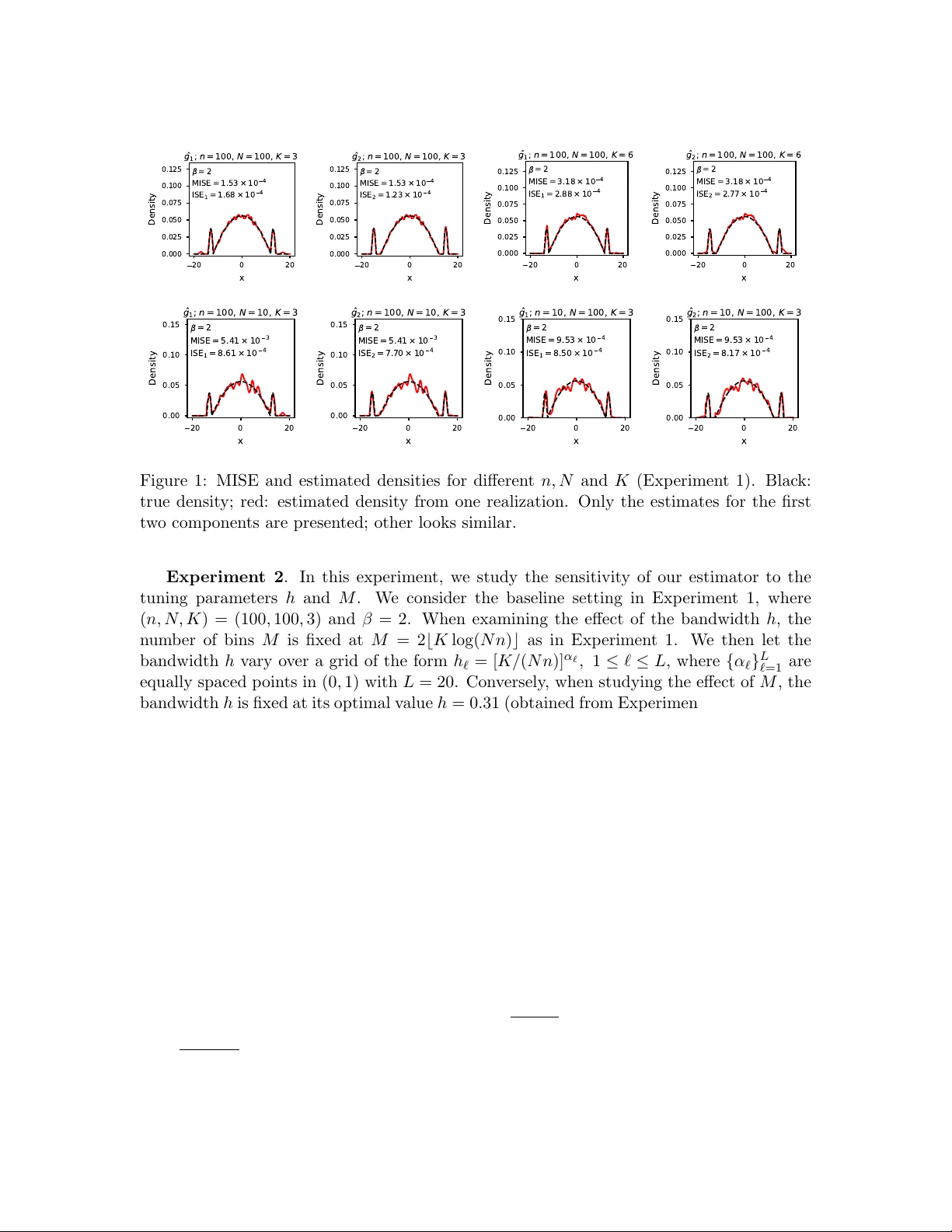
Optimal Demixing of Nonparametric Densities Jianqing F an jqf an@princeton.edu Dep artment of Op er ations R ese ar ch and Financial Engine ering Princ eton University Zheng T racy Ke zke@f as.har v ard.edu Dep artment of Statistics Harvar d University Zhao yang Shi zshi@f as.har v ard.edu Dep artment of Statistics Harvar d University Abstract Motiv ated by applications in statistics and machine learning, w e consider a problem of unmixing conv ex com binations of nonparametric densities. Supp ose we observe n groups of samples, where the i th group consists of N i indep enden t samples from a d -v ariate density f i ( x ) = P K k =1 π i ( k ) g k ( x ). Here, eac h g k ( x ) is a nonparametric density , and each π i is a K - dimensional mixed mem b ership v ector. W e aim to estimate g 1 ( x ) , . . . , g K ( x ). This problem generalizes topic mo deling from discrete to contin uous v ariables and ﬁnds its applications in LLMs with w ord em b eddings. In this pap er, w e propose an estimator for the abov e problem, which mo diﬁes the classical kernel densit y estimator b y assigning group-sp eciﬁc weigh ts that are computed b y topic mo deling on histogram vectors and de-biased by U-statistics. F or any β > 0, assuming that each g k ( x ) is in the Nikol’ski class with a smooth parameter β , we sho w that the sum of integrated squared errors of the constructed estimators has a conv ergence rate that dep ends on n , K , d , and the p er-group sample size N . W e also provide a matching lo wer b ound, which suggests that our estimator is rate-optimal. Keyw ords: Arc hetypal analysis, incomplete U statistics, kernel density estimation, min- imax analysis, topic modeling Con tents 1 In tro duction 3 1.1 Wh y classical approac hes do not work . . . . . . . . . . . . . . . . . . . . . 4 1.2 The induced topic mo dels . . . . . . . . . . . . . . . . . . . . . . . . . . . . 5 1.3 A new estimator . . . . . . . . . . . . . . . . . . . . . . . . . . . . . . . . . 5 1.4 The minimax optimal rate . . . . . . . . . . . . . . . . . . . . . . . . . . . . 6 1.5 Summary , organization and notations . . . . . . . . . . . . . . . . . . . . . 7 2 T opic-W eigh ted Kernel Density Estimator 7 2.1 An oracle estimator when Π is known . . . . . . . . . . . . . . . . . . . . . 7 2.2 Estimation of Π and the plug-in estimator . . . . . . . . . . . . . . . . . . . 8 2.3 De-biasing the plug-in estimator . . . . . . . . . . . . . . . . . . . . . . . . 9 2.4 The choice of tuning parameters and bins . . . . . . . . . . . . . . . . . . . 10 1 Jianqing F an, Zheng Tracy Ke, Zhao y ang Shi 2.5 Comparison with existing estimators . . . . . . . . . . . . . . . . . . . . . . 12 3 T opic Mo deling: Bac kground and Algorithms 13 3.1 T opic mo deling algorithms and their error rates . . . . . . . . . . . . . . . . 13 3.2 The T opic-SCORE algorithm . . . . . . . . . . . . . . . . . . . . . . . . . . 14 4 Main Results 14 4.1 Regularit y conditions . . . . . . . . . . . . . . . . . . . . . . . . . . . . . . . 15 4.2 A p erturbation b ound for our estimator . . . . . . . . . . . . . . . . . . . . 16 4.3 The error for estimating G . . . . . . . . . . . . . . . . . . . . . . . . . . . . 17 4.4 The rate of conv ergence of our estimator . . . . . . . . . . . . . . . . . . . . 17 4.5 A matching low er b ound . . . . . . . . . . . . . . . . . . . . . . . . . . . . . 18 4.6 Extension to a general d . . . . . . . . . . . . . . . . . . . . . . . . . . . . . 19 5 Sim ulations 20 6 Pro of of the Minimax Upp er Bound 22 6.1 Preliminaries . . . . . . . . . . . . . . . . . . . . . . . . . . . . . . . . . . . 23 6.2 A decomp osition of the error . . . . . . . . . . . . . . . . . . . . . . . . . . 23 6.3 The non-sto chastic ‘bias’ term . . . . . . . . . . . . . . . . . . . . . . . . . . 24 6.4 The main sto chastic error . . . . . . . . . . . . . . . . . . . . . . . . . . . . 25 6.5 The secondary sto chastic error, and pro of of Theorem 4.1 . . . . . . . . . . 27 7 Pro of sk etch of the Minimax Low er Bound 28 8 Discussion 30 A Analysis of our estimator 31 A.1 General to ols . . . . . . . . . . . . . . . . . . . . . . . . . . . . . . . . . . . 31 A.2 A useful lemma and its pro of . . . . . . . . . . . . . . . . . . . . . . . . . . 31 A.3 Proof of Lemma 6.3 . . . . . . . . . . . . . . . . . . . . . . . . . . . . . . . 33 A.4 Proof of Lemma 6.4 . . . . . . . . . . . . . . . . . . . . . . . . . . . . . . . 35 A.5 Proof of Lemma 6.1 . . . . . . . . . . . . . . . . . . . . . . . . . . . . . . . 35 A.6 Proof of Lemma 6.5 . . . . . . . . . . . . . . . . . . . . . . . . . . . . . . . 36 A.7 Proof of Lemma 6.2 . . . . . . . . . . . . . . . . . . . . . . . . . . . . . . . 38 A.8 Proof of Lemma 6.6 . . . . . . . . . . . . . . . . . . . . . . . . . . . . . . . 39 A.9 Proof of Lemma 6.7 . . . . . . . . . . . . . . . . . . . . . . . . . . . . . . . 43 A.10 Proof of Lemma 6.9 . . . . . . . . . . . . . . . . . . . . . . . . . . . . . . . 46 A.11 Proof of Lemma 6.10 . . . . . . . . . . . . . . . . . . . . . . . . . . . . . . . 46 A.12 Proof of Lemma 6.11 . . . . . . . . . . . . . . . . . . . . . . . . . . . . . . . 50 A.13 Proof of Theorem 4.2 . . . . . . . . . . . . . . . . . . . . . . . . . . . . . . . 52 A.13.1 Pro of of Theorem A.2 . . . . . . . . . . . . . . . . . . . . . . . . . . 56 A.13.2 Pro of of Theorem A.3 . . . . . . . . . . . . . . . . . . . . . . . . . . 62 A.13.3 Pro of of Theorem A.4 . . . . . . . . . . . . . . . . . . . . . . . . . . 62 A.14 Proof of Theorem 4.3 . . . . . . . . . . . . . . . . . . . . . . . . . . . . . . . 62 2 Unmixing Nonp arametric Densities B Pro of of the lo wer b ound 63 B.1 Pro of of Theorem 4.4 . . . . . . . . . . . . . . . . . . . . . . . . . . . . . . . 63 C Extension to the case of a general d 70 C.1 Pro of of Theorem C.1 . . . . . . . . . . . . . . . . . . . . . . . . . . . . . . 70 1 In tro duction Linear unmixing is a technique widely used in hypersp ectral imaging ( Bioucas-Dias et al. , 2012 ), chemical engineering ( Kwan et al. , 2006 ; Ayhan et al. , 2015 ), and biomedical data analysis ( Dey et al. , 2017 ; W ang and Zhao , 2022 ). Given n data p oin ts, it aims to ﬁnd K base vectors (‘end mem b ers’) such that eac h data p oin t is a conv ex com bination of base vectors, where K is often muc h smaller than n . In this pap er, w e consider a linear unmixing problem on the space of nonparametric densities. Supp ose f 1 ( x ) , . . . , f n ( x ) and g 1 ( x ) , . . . , g K ( x ) are densities on R d satisfying that f i ( x ) = K X k =1 π i ( k ) g k ( x ) , for 1 ≤ i ≤ n, (1.1) where each π i tak es v alue in the standard probability simplex S 0 ⊂ R K (i.e., the en tries of π i are nonzero and sum to 1). W e further assume that N i samples are drawn from eac h f i ( x ): X i 1 , X i 2 , . . . , X iN i iid ∼ f i ( x ) . (1.2) The goal is to use { X ij } 1 ≤ i ≤ n, 1 ≤ j ≤ N i to estimate the base densities g 1 ( x ) , . . . , g K ( x ). When K = 1, all X ij ’s are independent samples from a single density g 1 ( x ), so the problem reduces to classical nonparametric density estimation. When K > 1, ho wev er, the setting is fundamen tally diﬀeren t, with few results in the literature. In this pap er, we dev elop both new metho dology and minimax theory for the ab ov e problem. Our study is motiv ated by sev eral application examples: • T opic mo deling with wor d emb e ddings : T raditional topic mo deling is based on word coun t data. Modern large language models (LLMs) pro vide word embeddings that con tain ric her information than w ord coun ts. Recently , Austern et al. ( 2025 ) in tro duce a new topic mo del that is equiv alent to ( 1.1 )-( 1.2 ), where X ij is the con textualized w ord em b edding of the j th word in the i th do cument, and each g k ( x ) represents an abstract “topic”, depicting the distribution of the word em b edding in topic k . The estimated g 1 ( x ) , . . . , g K ( x ) are useful for uncov ering the underlying topic structure in a corpus. • Ar chetyp al analysis on distributional data : Archet ypal analysis ( Cutler and Breiman , 1994 ) aims to express n data p oin ts as conv ex com binations of K laten t archet yp es. In the original setting, ‘data’ and ‘archet yp es’ are feature v ectors, but in certain applications they can b e distributional data ( Bauckhage and Manshaei , 2014 ; W u and T abak , 2017 ). Existing metho ds typically apply the kernel tric k, but the formulation in ( 1.1 )-( 1.2 ) provides an alternative solution to archet ypal analysis on distributional data. 3 Jianqing F an, Zheng Tracy Ke, Zhao y ang Shi • De c ontamination of mutual c ontamination mo dels : Katz-Sam uels et al. ( 2019 ) con- sider mutual con tamination mo dels, in which a learner observes random samples from diﬀeren t conv ex com binations of a set of unknown base distributions. The goal is to infer the base distributions (i.e., decontamination). Our mo del in ( 1.1 )-( 1.2 ) can b e viewed a sp ecial mutual contamination mo del, where each base distribution has a con tinuous density . The decontamination problem has several applications, such as in multi-source domain adaption ( Zhan et al. , 2024 ) 1.1 Wh y classical approac hes do not work Kernel densit y estimator (KDE) is a text-b o ok metho d for nonparametric density estima- tion. It assumes that i.i.d. samples are observed from the density to b e estimated. Let K ( · ) b e a k ernel function suc h that R K ( x ) dx = 1, and write K h ( x ) := 1 h d K  1 h x  for brevit y . In ligh t of ( 1.2 ), the KDE for f i ( x ) is ˆ f KDE i ( x ) = 1 N i N i X j =1 K h ( X ij − x ) , 1 ≤ i ≤ n. (1.3) Ho wev er, ho w to use ˆ f KDE 1 ( x ) , . . . , ˆ f KDE n ( x ) to estimate g 1 ( x ) , . . . , g K ( x ) is unclear. More- o ver, the rate of estimating each f i ( x ) only dep ends on N i , but w e exp ect a muc h faster rate of conv ergence on estimating g k ( x ), which should dep end on P n i =1 N i . In the mixture densit y estimation (MDE) problem, we observe i.i.d. samples from a den- sit y f ( x ) = P K k =1 β k g ( x ; λ k ), where g ( x ; λ ) is a parametric densit y family , and β 1 , β 2 , . . . , β K are the mixing weigh ts. This mo del can b e recast as a latent v ariable mo del and solv ed by the exp ectation-maximization (EM) algorithm. In a similar spirit, w e introduce a paramet- ric version of the mo del in ( 1.1 )-( 1.2 ) by π 1 , . . . , π n iid ∼ Diric hlet( α ) , X i 1 , . . . , X iN i | π i iid ∼ f i ( x ) = K X k =1 π i ( k ) g ( · ; λ k ) , (1.4) and the parameters can b e estimated by the v ariational EM algorithm ( Blei and Jordan , 2004 ). Unfortunately , this requires eac h g k ( x ) to hav e a parametric form. There exist approaches that approximate a nonparametric density b y parametric ones, primarily for the case of estimating a single densit y g ( x ). The Dirichlet Pro cess Mixture Mo del (DPMM) ( Escobar and W est , 1995 ) expresses a nonparametric densit y as an inﬁnite mixture of parametric densities, with mixing w eights generated from a ‘stic k-breaking con- struction’ pro cess. The v ariational auto-enco der (V AE) expresses a nonparametric densit y as an inﬁnite mixture of normal densities ( Demange-Chryst et al. , 2023 ), parametrized by neural netw orks. Ho wev er, if w e use these ideas to extend the model in ( 1.4 ) to a non- parametric version, several issues arise: Ho w to design a v alid estimation procedure? Is the obtained ˆ g k ( x ) smooth? What rate of con vergence can b e guaran teed? There are no clear answ ers. In the mac hine learning literature, Katz-Sam uels et al. ( 2019 ) prop ose an interesting metho d for estimating g 1 ( x ) , . . . , g K ( x ) when n = K . Let ˆ F i ( x ) b e the empirical distri- bution asso ciated with X i 1 , . . . , X iN i . This metho d computes the “residual” of eac h ˆ F i 4 Unmixing Nonp arametric Densities after remo ving a maximal linear eﬀect of { ˆ F j : j  = i } . These “residuals” are then used to construct estimators of base distributions. How ev er, the estimated distributions typically do not admit smo oth densities; moreo v er, this metho d relies on strong conditions on the mixing weigh ts π i , which may be hard to satisfy in practice. 1.2 The induced topic mo dels In terestingly , the model in ( 1.1 )-( 1.2 ) has a connection to the topic model ( Blei et al. , 2003 ), whic h is widely used in text analysis. In detail, ﬁx a partition of R d in to M bins, R d = ∪ M m =1 B m , (1.5) and construct a ‘multiv ariate histogram’ vector Y i ∈ R M for the i th group of samples by Y i ( m ) = |{ X ij : 1 ≤ j ≤ N i } ∩ B m | , 1 ≤ m ≤ M . (1.6) F ollowing ( 1.2 ), it is easy to see that Y i ∼ Multinomial( N i , Ω B i ), where Ω B i ∈ R M is a vector suc h that Ω B i ( m ) = R x ∈B m f i ( x ) dx . Com bining this with the expression of f i ( x ) in ( 1.1 ), w e immediately hav e the follo wing result: Y i ∼ Multinimial  N i , K X k =1 π i ( k ) g B k  , where g B k ( m ) = Z x ∈B m g k ( x ) dx. (1.7) This is in fact a topic mo del with n do cumen ts, K topics, and a size- M v o cabulary , where g B 1 , . . . , g B K ∈ R M are the “topic v ectors” and π 1 , . . . , π n ∈ R K are the “topic w eight vectors.” Inspired by this connection, Austern et al. ( 2025 ) prop ose a tw o-step metho d for esti- mating the densities g 1 ( x ) , . . . , g K ( x ): • Apply topic mo deling on the matrix Y = [ Y 1 , Y 2 , . . . , Y n ] to obtain ˆ g B 1 , . . . , ˆ g B K . • F or eac h 1 ≤ k ≤ K , construct ˆ g k ( x ) from the entries of ˆ g B k b y k ernel smo othing. This pro vides the ﬁrst metho d for the nonparametric linear unmixing problem in ( 1.1 )-( 1.2 ) with a pro v able rate of con vergence. Unfortunately , the rate do es not match the information- theoretic low er b ound when g 1 ( x ) , . . . , g K ( x ) hav e high smo othness (see Section 4.4 ). In this paper, w e introduce a new estimator, which also lev erages the induced topic mo del in ( 1.7 ), but in a fundamentally diﬀeren t manner. W e show that the new estimator addresses the ab ov e limitation and is minimax optimal. 1.3 A new estimator Let Y b e the same as deﬁned in ( 1.6 ). Suppose we hav e applied an existing topic mo deling algorithm on Y , and let b G = [ ˆ g B 1 , . . . , ˆ g B K ] be the estimated topic matrix. Our estimator is inspired by several k ey insights: • First, w e consider an idealized case where π 1 , . . . , π n are known. In this case , w e construct an ideal estimator for g k ( x ), whic h is a weigh ted KDE b y leveraging these kno wn π i ’s. 5 Jianqing F an, Zheng Tracy Ke, Zhao y ang Shi • Next, we develop an estimator of π 1 , . . . , π n based on the estimated topic matrix b G and w e plug ˆ π 1 , . . . , ˆ π n in to the ideal estimator. This is a natural plug-in estimator for g k ( x ), but unfortunately it has a large bias. • Finally , we de-bias the ab ov e plug-in estimator b y replacing some quadratic terms b y corresp onding U-statistics. The detailed deriv ation and rationale are deferred to Section 2 , but let us describe the estimator ﬁrst. With the notation in ( 1.5 )-( 1.6 ), w e deﬁne a matrix T ∈ R M × M with elemen ts T mm ′ = n X i =1 1 N i ( N i − 1) X 1 ≤ j  = j ′ ≤ N i U ij m U ij ′ m ′ , where U ij m = 1 { X ij ∈ B m } . (1.8) F or any x ∈ R d , we deﬁne a matrix S ( x ) ∈ R M × n b y S mi ( x ) = 1 N i ( N i − 1) X 1 ≤ j  = j ′ ≤ N i K ij ( x ) U ij ′ m , where K ij ( x ) = K h ( x − X ij ) , (1.9) where K h is deﬁned in ( 1.3 ). Our prop osed estimator has the form: b g ( x ) = b G ′ b G ( b G ′ T b G ) − 1 b G ′ S ( x ) 1 n , (1.10) where for each 1 ≤ k ≤ K , ˆ g k ( x ) is the k th entry of b g ( x ). Here, eac h ˆ g k ( x ) is a w eighted U-statistic, with weigh ts dep ending on the estimated topic matrix b G . It has an en tirely diﬀerent form from the estimator in Austern et al. ( 2025 ). As a consequence, the choice of the bin size M is also fundamentally diﬀerent. They choose M as a p ow er of N n , whereas we simply set M ≍ K log ( N n ); see Section 2 . 1.4 The minimax optimal rate F or any ﬁxed β > 0, let Θ ∗ β denote the Nik ol’ski class ( Nikol’skii , 2012 ) of smo oth probability densities with a smo othness parameter β . W rite for brevity g ( x ) = ( g 1 ( x ) , . . . , g K ( x )) ′ and b g ( x ) = ( ˆ g 1 ( x ) , . . . , ˆ g K ( x )) ′ . W e denote g ( x ) ∈ Θ ∗ β when eac h individual g k ( x ) belongs to the Nikol’ski class. One of our main results is the minimax rate of conv ergence for the in tegrated squared error: Supp ose N i ≍ N for 1 ≤ i ≤ n . As nN → ∞ , if K = O (( N n ) c ∗ β ,d ), where c ∗ β ,d ∈ (0 , 1 / 4) is a constant that only dep ends on β , then up to a p ermutation of ˆ g 1 ( x ) , . . . , ˆ g K ( x ), inf b g ( x ) sup g ( x ) ∈ Θ ∗ β E " K X k =1 Z [ ˆ g k ( x ) − g k ( x )] 2 dx # ≍ K  K N n  2 β 2 β + d . (1.11) T o establish ( 1.11 ), w e need a minimax upp er b ound and a minimax low er b ound. The minimax upper b ound is obtained b y analyzing the error rate of our estimator. In the proof, w e hav e developed a large-deviation inequality for a sp eciﬁc class of incomplete U-statistics and an integrated v ariance b ound for incomplete U-pro cesses. The minimax low er b ound is prov ed b y choosing a least-fa v orable conﬁguration to uncov er the role of a div erging K . 6 Unmixing Nonp arametric Densities 1.5 Summary , organization and notations W e consider unmixing conv ex combinations of nonparametric densities, a problem with ap- plications in topic mo deling, archet ypal analysis and multi-source domain adaption. Com- pared to classical nonparametric density estimation, this problem is more challenging and m uch less studied. Our con tributions include: • W e prop ose a new estimator, which are signiﬁcantly diﬀerent from existing metho ds (e.g., Katz-Samuels et al. ( 2019 ); Austern et al. ( 2025 )). • W e derive an explicit rate of conv ergence for our estimator. Our results allow b oth N and K to grow with n and cov er a full range of smo othness on the base densities. • W e pro vide a matc hing lo w er b ound and show that our estimator is optimal. In con trast, existing estimators either hav e no explicit error rate or suﬀer a non-optimal rate. • As a component of our analysis, w e also pro vide a new theoretical result on estimating a topic mo del under a gro w ing K , which is of indep endent interest. The remainder of this pap er is organized as follows: In Section 2 , we deriv e our esti- mator and explain the insights. Section 3 discusses the topic mo deling on Y , fo cusing an existing algorithm T opic-SCORE. Our main theoretical results are presented in Section 4 . Sim ulation studies are contained in Section 5 . Sections 6 - 7 pro ve the minimax upp er b ound and the minimax lo wer bound, resp ectively . Section 8 concludes the pap er with discussions. Pro ofs of secondary lemmas are relegated to the s upplemen tary material. 2 T opic-W eigh ted Kernel Densit y Estimator In this section, we explain the rationale of our prop osed estimator ( 1.10 ). W e show that it is equiv alent to a de-biased w eighted kernel densit y estimator with estimated w eights from topic mo deling. 2.1 An oracle estimator when Π is known W e ﬁrst consider an oracle setting where the mixed membership matrix Π = [ π 1 , . . . , π n ] ′ ∈ R n × K is giv en. Let g ( x ) = ( g 1 ( x ) , . . . , g K ( x )) ′ ∈ R K and f ( x ) = ( f 1 ( x ) , . . . , f n ( x )) ′ ∈ R n . It follows from the mo del in ( 1.1 ) that f ( x ) = Π g ( x ) or g ( x ) = (Π ′ Π) − 1 Π ′ f ( x ) The unknown density vector f ( x ) can be estimated b y b f KDE ( x ) = ( ˆ f KDE 1 ( x ) , . . . , ˆ f KDE n ( x )) ′ , where ˆ f KDE i ( x ) is given by ( 1.3 ). This leads naturally to b g oracle ( x ) = (Π ′ Π) − 1 Π ′ b f KDE ( x ) . The k th comp onen t of the ab ov e estimator can b e written as ˆ g oracle k ( x ) = 1 n n X i =1 b i ( k ) ˆ f KDE i ( x ) , (2.1) 7 Jianqing F an, Zheng Tracy Ke, Zhao y ang Shi where b i ( k ) is given b y B = ( n − 1 Π ′ Π) − 1 Π ′ := [ b 1 , b 2 , . . . , b n ] ∈ R K × n . (2.2) It is the weigh t on the i th group of samples when they are used to estimate g k ( x ). Putting more explicitly , w e prop ose a w eigh ted k ernel density estimator (KDE): ˆ g oracle k ( x ) = 1 n n X i =1 b i ( k ) 1 N i N i X j =1 K h ( x − X ij ) , 1 ≤ k ≤ K, (2.3) The rate of con vergence of this oracle estimator can b e fairly easily deriv ed (see the supplemen t), and it matches the low er b ound to b e introduced in Section 4 . W e thereby use this estimator as a go o d starting p oint. 2.2 Estimation of Π and the plug-in estimator T o extend the oracle estimator to the real case, we need an estimate of Π. In ligh t of the induced topic mo del in ( 1.7 ), we can apply topic mo deling to Y . How ever, if we directly apply an existing topic mo deling algorithm on estimating Π, the rate of conv ergence is not fast enough. Assuming K is ﬁnite, the minimax optimal rate is ( Klopp et al. , 2023 ; W u et al. , 2023 ) max 1 ≤ i ≤ n ∥ ˆ π i − π i ∥ 1 = O P  N − 1 / 2  . This rate do es not ev en decrease with n ; consequen tly , the plug-in error caused by estimating Π is to o large. In order to get the desirable rate, w e m ust accoun t for the dependence among ˆ π i ’s. This is made p ossible if eac h ˆ π i can b e well-appro ximated by a simple function of X . (2.4) T o ﬁnd an estimator to satisfy ( 2.4 ), we notice that, while the rate on estimating π i is slo w, the rate on estimating the topic matrix G can be made very fast. In fact, the minimax optimal rate ( Ke and W ang , 2024b ; Bing et al. , 2020 ) is K X k =1 ∥ ˆ g k − g k ∥ 1 = e O P K r K M N n ! . (2.5) Here, M is the bin size that a user can choose. If w e c ho ose M appropriately small, then the rate on estimating G can b e muc h faster than the optimal rate in ( 1.11 ), so that we can almost treat G as kno wn. The ab o ve observ ation inspires us to consider a regression estimator of Π. In detail, let L ∈ R n × n b e a diagonal matrix whose i th diagonal entry is equal to N i . It follows from ( 1.7 ) that E Y = G Π ′ L . W e thereby estimate Π by b Π = L − 1 Y ′ b G ( b G ′ b G ) − 1 . (2.6) Since the plug-in error rate in b G is muc h faster than the desirable rate, we can almost treat G as known and appro ximate the b Π in ( 2.6 ) by b Π ≈ b Π ∗ := L − 1 Y ′ G ( G ′ G ) − 1 . (2.7) 8 Unmixing Nonp arametric Densities The righ t hand side of ( 2.7 ) is a linear function of Y , and Y is constructed from X ij ’s explicitly . Hence, the estimator b Π satisﬁes ( 2.4 ) as w e hop e. Note that this estimator does not yield a faster rate on estimating Π than existing estimators (e.g., Klopp et al. ( 2023 ); W u et al. ( 2023 )). The adv antage lies in a voiding a ma jor analytical h urdle when w e use b Π to construct other estimators: Since the dep endence among ˆ π 1 , . . . , ˆ π n can b e quan tiﬁed explicitly as in ( 2.7 ), w e obtain a m uch tighter con trol on the plug-in error. On the other hand, this adv antage is tied to our problem: As the c hoice of bins v ary , we hav e man y induced topic mo dels, and all of them share the same Π. This gives us the freedom to pick a prop er induced topic mo del so that ( 2.7 ) holds. W e now plug the b Π in ( 2.6 ) into the oracle estimator in ( 2.2 )-( 2.3 ). W rite for brevity b Q := b G ( b G ′ b G ) − 1 , f W := n ( b Q ′ Y L − 2 Y ′ b Q ) − 1 b Q ′ . (2.8) W e use ˜ w ′ i ∈ R K to denote the i th ro w of f W . It is not hard to see that the plug-in estimator has the following form: ˆ g plug-in k ( x ) := 1 n n X i =1 1 N 2 i N X j =1 M X m =1 ˜ w m ( k ) K h ( x − X ij ) Y i ( m ) , 1 ≤ k ≤ K. (2.9) W e write b g plug-in ( x ) = ( ˆ g plug-in 1 ( x ) , . . . , ˆ g plug-in K ( x )) ′ for brevity . 2.3 De-biasing the plug-in estimator Unfortunately , the plug-in estimator in ( 2.9 ) has a non-negligible bias. In this subsection, w e explain where the bias comes from and in tro duce a de-biasing tec hnique. The following lemma is prov ed in the supplemental material: Lemma 2.1. L et R d = ∪ M m =1 B m b e the bins and b Q b e as in ( 2.8 ) . Write U ij m = 1 { X ij ∈ B m } , for al l 1 ≤ i ≤ n , 1 ≤ j ≤ N i and 1 ≤ m ≤ M . Then, the plug-in estimator in ( 2.9 ) satisﬁes that b g plug-in ( x ) = e Σ − 1 e h ( x ) , wher e e h ( x ) ∈ R K and e Σ ∈ R K × K ar e deﬁne d by e h k ( x ) = 1 n n X i =1 1 N 2 i M X m =1 N i X j,j ′ =1 b Q mk K h ( x − X ij ) U ij ′ m , 1 ≤ k ≤ K, e Σ kℓ = 1 n n X i =1 1 N 2 i M X m,m ′ =1 N i X j,j ′ =1 b Q mk b Q m ′ ℓ U ij m U ij ′ m ′ , 1 ≤ k , ℓ ≤ K . Lemma 2.1 gives an equiv alent form of the plug-in estimator. W e ﬁrst study the matrix e Σ . Let U ij ∈ R M b e the v ector consisting of { U ij m : 1 ≤ m ≤ M } . F or eac h i , U i 1 , . . . , U iN i are i.i.d. from Multinomial(1 , ξ i ), with ξ i := E [ U i 1 ]. It is seen that e Σ = b Q ′  1 n n X i =1 d ξ i ξ ′ i  b Q, where d ξ i ξ ′ i := 1 N 2 i N i X j,j ′ =1 U ij U ′ ij ′ . Ho wev er, E [ U ij U ′ ij ′ ]  = ξ i ξ ′ i when j = j ′ . Therefore, the estimator d ξ i ξ ′ i is biased. T o ﬁx this issue, w e consider the follo wing U-statistics, which employ a diagonal deletion strategy by 9 Jianqing F an, Zheng Tracy Ke, Zhao y ang Shi excluding j = j ′ in the sum: d ξ i ξ ′ i ∗ := 1 N i ( N i − 1) X 1 ≤ j  = j ′ ≤ N i U ij U ′ ij ′ . This is an un biased estimator of ξ i ξ ′ i . Replacing d ξ i ξ ′ i b y this estimator gives a mo diﬁcation of e Σ in ( 2.10 ) b elow. W e also mo dify e h k ( x ) by a similar diagonal deletion strategy . Let b h ( x ) ∈ R K and b Σ ∈ R K × K b e such that b h k ( x ) = 1 n n X i =1 1 N i ( N i − 1) M X m =1 X 1 ≤ j  = j ′ ≤ N i b Q mk K h ( x − X ij ) U ij ′ m , 1 ≤ k ≤ K, b Σ kℓ = 1 n n X i =1 1 N i ( N i − 1) M X m,m ′ =1 X 1 ≤ j  = j ′ ≤ N i b Q mk b Q m ′ ℓ U ij m U ij ′ m ′ , 1 ≤ k , ℓ ≤ K . (2.10) Our ﬁnal estimator of g ( x ) is the diagnonal deletion version: b g ( x ) = ( ˆ g 1 ( x ) , . . . , ˆ g K ( x )) ′ := b Σ − 1 b h ( x ) . (2.11) Recall that b Q = b G ( b G ′ b G ) − 1 and Q = G ( G ′ G ) − 1 . Using the matrices S and T deﬁned in ( 1.8 )-( 1.9 ), we can re-express b h ( x ) and b Σ in ( 2.10 ) b y b h ( x ) = n − 1 b Q ′ S ( x ) 1 n = n − 1 ( b G ′ b G ) − 1 b G ′ S ( x ) 1 n , b Σ = n − 1 b Q ′ T b Q = n − 1 ( b G ′ b G ) − 1 b G ′ T b G ( b G ′ b G ) − 1 . (2.12) It follows immediately that b g ( x ) = b G ′ b G ( b G ′ T b G ) − 1 b G ′ S ( x ) 1 n . (2.13) This simpliﬁes the expression in ( 2.11 ), which is also the one we in tro duce in ( 1.10 ). 2.4 The choice of tuning parameters and bins Our metho d requires tw o tuning parameters, the bandwidth h and the bin size M . In addition, giv en M , we need to choose the bins B 1 , . . . , B M . In this subsection, we discuss ho w to determine them in practice. First, based on our theory in Section 4 , the optimal M is at the order of K log( N n ), whic h do es not dep end on unkno wn parameters. In Section 5 , we also observ e that the p erformance of our estimator is insensitiv e to M in a wide range (see Figure 2 ). W e th us ﬁx M as M = 2 ⌊ K log( N n ) ⌋ . (2.14) Next, we discuss how to choose the bins B 1 , . . . , B M . Let ¯ g ( x ) = 1 K P K k =1 g k ( x ). F or our theoretical analysis to carry through, w e hop e: Z x ∈B m ¯ g ( x ) dx ≍ 1 / M , for all bins B 1 , B 2 , . . . , B M . (2.15) 10 Unmixing Nonp arametric Densities When ¯ g ( x ) has a b ounded supp ort and is uniformly lo w er b ounded by a constant, w e can use a simple equi-size cubic bins, whic h guarantees ( 2.15 ). In the more general case where ¯ g ( x ) has unbounded supp ort, w e can sho w that as long as the K en tries of α = Π ′ diag( N 1 , . . . , N n ) 1 n are of the same order, ( 2.15 ) is equiv alent to E [# { X ij ∈ B m } ] ≍ ¯ N n/ M . (2.16) This inspires a practical c hoice of bins: we make sure that the total num b er of samples falling into each bin is of the order ¯ N n/ M . F or example, when d = 1, w e can sort X ij ’s and let δ m b e the m/ M quan tile. The bins are ( −∞ , δ 1 ] ∪ ( δ 1 , δ 2 ] ∪ . . . ∪ ( δ M − 2 , δ M − 1 ] ∪ ( δ M − 1 , ∞ ) . (2.17) Finally , w e describe ho w to select h . The optimal h dep ends on the unkno wn smoothness of base densities. Therefore, w e face the same challenge as in classical nonparametric density estimation. F ortunately , there is a careful study of bandwidth selection in that literature. One approach is to minimize the asymptotic mean integrated error squared error (AMISE), whic h can b e estimated by lea ve-one-out cross v alidation (abbreviated as CV; e.g., see Park ( 1993 )) or plug-in estimators (e.g., see Hall et al. ( 1991 )). Another approach is the Lepski’s metho d ( Lepskii , 1992 ), whic h takes an ordered sequence of h and ﬁnds ˆ h suc h that the resulting estimator do es not diﬀer to o m uch from all estimators from smaller bandwidths. W e can p ossibly extend these approac hes to our setting. F or con v enience, we only consider the CV approach. F ollo wing W asserman ( 2006 , Page 135-137), w e deﬁne AMSE as AMISE( h ; b g ) = Z ∥ b g ( x ) ∥ 2 dx − 2 Z  g ( x ) , b g ( x )  dx := Z ∥ b g ( x ) ∥ 2 dx − J ( h ; b g ) . Only the second term g ( x ) = B f ( x ) is unknown, where B = ( n − 1 Π ′ Π) − 1 Π ′ = [ b 1 , b 2 , . . . , b n ] is as in ( 2.2 ). Let { X ∗ ij } b e an indep enden t cop y of { X ij } . It is seen that J ( h ; b g ) = 2 n n X i =1 Z b ′ i b g ( x ) f i ( x ) dx = 2 n n X i =1 ( 1 N i N i X j =1 b ′ i E  b g ( X ∗ ij )  ) . Borro wing the CV idea, w e leav e-out each X ij and use the remaining samples to construct b g ( − ij ) . This also yields b Π − ( ij ) as an in termediate quantit y , whic h we plug in to ( 2.6 ) to obtain b B − ( ij ) = [ ˆ b 1( − ij ) , . . . , ˆ b n ( − ij ) ]. W e select h b y minimizing the follo wing criteria: \ AMISE( h ; b g ) = Z ∥ b g ( x ) ∥ 2 dx − 2 n n X i =1 " 1 N i N i X j =1 ˆ b ′ i ( − ij ) b g ( − ij ) ( X ij ) # . (2.18) This pro cedure requires conducting topic mo deling for P n i =1 N i times. T o sav e the com- putational cost, w e prop ose a mo diﬁed version that only runs topic mo deling once. Note that B = Σ − 1 Π ′ . W e plug in b Σ in ( 2.12 ) and b Π in ( 2.6 ) to get b B = n ( b G ′ b G )( b G ′ T b G ) − 1 b G ′ Y L − 1 . Here, only b G comes from topic mo deling. Similarly , in the expression of b g in ( 2.13 ), only b G comes from topic mo deling. Therefore, we use all data to obtain b G but p erform lea ve-one- out in the remaining quan tities. This gives the follo wing lea ve-one-out estimators: e B ( − ij ) = n ( b G ′ b G )  b G ′ T ( − ij ) b G  − 1 b G ′ ( Y L − 1 ) − ( ij ) , 11 Jianqing F an, Zheng Tracy Ke, Zhao y ang Shi e g − ( ij ) ( x ) = b G ′ b G  b G ′ T ( − ij ) b G  − 1 b G ′ S ( − ij ) ( x ) 1 n , (2.19) where T ( − ij ) , S ( − ij ) ( x ) and ( Y L − 1 ) − ( ij ) are the corresp onding leav e-one-out v ersions of T , S ( x ) and Y L − 1 , resp ectively . Let ^ AMISE( h ; b g ) b e a coun terpart of ( 2.18 ), where w e mo dify the second term using the quantities in ( 2.19 ). W e select h by minimizing ^ AMISE( h ; b g ). This pro cedure only requires conducting topic mo deling once. 2.5 Comparison with existing estimators There are few existing methods for our problem. Katz-Samuels et al. ( 2019 ) consider a similar mo del where the base distributions do not necessarily ha ve smo oth densities. They deﬁne a quantit y κ ∗ ( f i |{ f j , j  = i } ) = max  κ ∈ [0 , 1] : there exists R i suc h that f i = κR i + P j  = i ν j f j for some ν j ≥ 0 with P j  = i ν j = 1 − κ.  The resulting R i is also a distribution and called a “residual” of f i . Katz-Samuels et al. ( 2019 ) show that R i can b e estimated from the empirical CDFs ˆ F 1 , . . . , ˆ F n . They also show that when n = K and when Π satisﬁes certain conditions, the base distributions can b e reco vered b y recursively computing such “residuals.” The k ey insight is to exploit a simplex geometry in the distribution space. Ho wev er, this approac h imp oses restrictive conditions on Π, which essen tially requires that each π i is close to b eing degenerate. In con trast, our metho d bypasses this limitation b y considering the induced topic mo del. While topic modeling also relies on a simplex geometry , the geometry arises in the standard Euclidean space, whic h can b e eﬀectiv ely exploited using existing topic mo deling algorithms, hence requiring very mild conditions on Π. In theory , Katz-Sam uels et al. ( 2019 ) only establish a consistency guarantee but do not pro vide an y explicit rate of conv ergence. In contrast, we not only derive the explicit rate of con vergence for our estimator but also sho w that it is minimax optimal. Our method is connected to the one in Austern et al. ( 2025 ) in lev eraging the induced topic mo del. How ever, the tw o metho ds diﬀer fundamen tally in how to use the estimated topic mo del. Austern et al. ( 2025 ) treat the topic matrix G as a “discretization” of the con tinuous densities g 1 ( x ) , . . . , g K ( x ). The bin size M leads to a bias-v ariance trade-oﬀ: on one hand, M needs to b e properly large so that G con tains suﬃcien t information of g 1 ( x ) , . . . , g K ( x ); on the other hand, since M aﬀects the estimation error on G , it cannot b e to o large. Unfortunately , in some parameter regime (e.g., when β > 1), there do es not exist a sweet sp ot of M . This explains why their metho d cannot b e optimal across the whole parameter regime. In con trast, our estimator builds on the oracle estimator in ( 2.3 ), which is already minimax optimal across the whole parameter regime. W e only need to dev elop a b Π such that the plug-in error is negligible. This seems c hallenging, as Π is a large matrix. F ortunately , w e leverage the induced topic mo del to design a b Π in whic h the dependence among its en tries can b e well c haracterize d. This allows us to hav e a sharp control of the plug-in error and ev entually prov e that our estimator has the same error rate as the oracle estimator, th us being optimal. 12 Unmixing Nonp arametric Densities 3 T opic Mo deling: Bac kground and Algorithms One step in our estimator is to conduct topic mo deling on the matrix Y . In this section, we review the topic mo del and existing topic modeling algorithms. In particular, w e describ e T opic-SCORE ( Ke and W ang , 2024b ), the algorithm we use in our n umerical exp eriments and theoretical analysis. 3.1 T opic mo deling algorithms and their error rates Supp ose we observ e n do cuments written on a vocabulary of M w ords. Let Y i ∈ R M b e the w ord count vector for the i th do cument, where Y i ( m ) is the coun t of the m th word, and N i = P M m =1 Y i ( m ) is the total length of this do cument. Let g 1 , g 2 , . . . , g K ∈ R M b e K topic v ectors, eac h b eing a probability mass function (PMF) and represen ting a discrete distribution on the v o cabulary . Eac h do cument i is asso ciated with a topic weigh t vector π i ∈ R K , where π i ( k ) is the fractional weigh t this document puts on the k th topic, for 1 ≤ k ≤ K . The topic mo del assumes that Y 1 , Y 2 , . . . , Y n are indep endent, and Y i ∼ Multinomial( N i , Ω i ) , Ω i = K X k =1 π i ( k ) g k . (3.1) The goal of topic mo deling is to use the data matrix Y = [ Y 1 , . . . , Y n ] to estimate the parameters G = [ g 1 , . . . , g K ] and Π = [ π 1 , . . . , π n ] ′ . There are many existing metho ds for this problem. They can b e roughly divided into t wo categories depending on the k ey assumption: In the ﬁrst category , it is assumed that π i ’s are i.i.d. from a Dirichlet prior. A p opular metho d in this category is the latent Dirichlet allo cation ( Blei et al. , 2003 ). In the second category , it is assumed that each topic has at least one anchor w ord, where a word m is an anchor word if the m th row of G has only one nonzero entry . Representativ e metho ds include the NMF approach ( Arora et al. , 2012 ), the T opic-SCORE algorithm ( Ke and W ang , 2024b ), and the LOVE algorithm ( Bing et al. , 2020 ). W e can plug in any of these algorithms in to our estimator. How ever, to achiev e the b est p erformance, we prefer a topic mo deling algorithm that has a fast rate of conv ergence. Deﬁne the ℓ 1 -error as (sub ject to a column permutation of b G ) L ( b G, G ) = X 1 ≤ m ≤ M X 1 ≤ k ≤ K | b G mk − G mk | . Assuming K is ﬁxed, Ke and W ang ( 2024a ) summarize the rates of conv ergence of L ( b G, G ) for diﬀeren t algorithms and ﬁnd that only T opic-SCORE ( Ke and W ang , 2024b ) and LOVE ( Bing et al. , 2020 ) attain the optima rate p M / ( ¯ N n ), up to logarithmic factors. In com- parison, LOVE requires that M ≪ ¯ N , while T opic-SCORE do es not hav e this requirement. When K gro ws with n , LOVE has the following rate of con vergence, L ( b G, G ) ≤ C ( ¯ N n ) − 1 / 2 q K 3 M log ( ¯ N n ) , (3.2) whic h is again under the assumption of M ≪ ¯ N . The rate of con vergence of T opic-SCORE for gro wing K has not b een given in the literature. In Section 4.3 , w e close this gap and 13 Jianqing F an, Zheng Tracy Ke, Zhao y ang Shi sho w that T opic-SCORE also attains the rate in ( 3.2 ); and this is true for b oth the case of M ≪ ¯ N and M = O ( ¯ N ). The rate in ( 3.2 ) is minimax optimal sub ject to a logarithm factor, according to the low er b ound in Bing et al. ( 2020 ). Based on these observ ations, w e recommend using T opic-SCORE. 3.2 The T opic-SCORE algorithm T opic-SCORE ( Ke and W ang , 2024b ) b elongs to the category of topic mo deling algorithms that assume the anchor w ord condition. A word 1 ≤ m ≤ M is called an anc hor word of topic k if and only if g k ( m )  = 0 , and g ℓ ( m ) = 0 for all ℓ  = k . (3.3) The anchor word condition requires that each topic has at least one anc hor word. W e now brieﬂy describ e the key idea b ehind T opic-SCORE. Let L = diag( N 1 , N 2 , . . . , N n ) and e Y = Y L − 1 . Let ˆ ξ 1 , . . . , ˆ ξ K ∈ R M b e the ﬁrst K left singular v ectors of e Y and deﬁne b R = [diag ( ˆ ξ 1 )] − 1 [ ˆ ξ 2 , . . . , ˆ ξ K ] ∈ R M × ( K − 1) . Ke and W ang ( 2024b ) sho w that there exists a lo w-dimensional K -v ertex simplex associated with the ro ws of b R . As long as each topic has at least one anchor word, this simplex can b e estimated from b R . Once this simplex is av ailable, it can b e used to obtain an explicit form ula for con verting the singular v ectors to v alid estimates of the topic v ectors. The full algorithm is as follows: 1. (SVD) . Let D = diag ( e Y 1 n ). Obtain the ﬁrst K left singular vectors D − 1 / 2 e Y , and denote them by ˆ ξ 1 , . . . , ˆ ξ K ∈ R M . Construct a matrix b R = [diag ( ˆ ξ 1 )] − 1 [ ˆ ξ 2 , . . . , ˆ ξ K ]. 2. (Simplex vertex hunting) . Apply a v ertex hun ting algorithm ( Ke and Jin , 2023 , Section 3.4) to the rows of b R to obtain ˆ v 1 , ˆ v 2 , . . . , ˆ v K . W rite b V = [ ˆ v 1 , ˆ v 2 , . . . , ˆ v K ]. 3. (T opic matrix estimation) . F or each 1 ≤ m ≤ M , obtain ˆ u m b y solving the equations: 1 ′ K ˆ u m = 1, and b V ˆ u m = ˆ r m . If ˆ u m con tains negativ e entries, set these en tries to zero and renormalize the whole vector to hav e a unit ℓ 1 -norm. F or eac h 1 ≤ k ≤ K , estimate g k b y normalizing the k th column of D 1 / 2 diag( ˆ ξ 1 )[ ˆ u 1 , ˆ u 2 , . . . , ˆ u M ] ′ to ha ve a unit ℓ 1 -norm. In Section 4.3 , we pro vide a tight error b ound for this algorithm, which extends the existing b ounds from ﬁxed K ( Ke and W ang , 2024a ) to growing K . This result is not only useful for the analysis of our estimator but also of indep enden t in terest. 4 Main Results In this section, w e presen t our main theoretical results. F or technical reasons, w e in tro duce a slightly mo diﬁed v ersion of the estimator in ( 1.10 ): b g + ( x ) = b G ′ b G  b G ′ T b G + ϵI K  − 1 b G ′ S ( x ) 1 n , (4.1) 14 Unmixing Nonp arametric Densities where ϵ = ϵ n = K n M 2 · 1  λ min ( b G ′ T b G ) < K n M 2 log 2 ( N n )  . In fact, λ min ( b G ′ T b G ) is often muc h larger than K n M 2 log 2 ( N n ) , so that b g + ( x ) and b g ( x ) are iden tical except for a negligible probability . Ho wev er, when we b ound the expected error of b g ( x ), w e m ust study the b eha vior of our estimator on this small-probabilit y ev ent, which is tec hnically c hallenging. T o a void this h urdle, w e study the ab o v e modiﬁed v ersion. In Sections 4.1 - 4.5 , we fo cus on d = 1, for which the regularity conditions and main results are b oth easy to presen t and in terpret. The extension to d > 1 is deferred to Section 4.6 . 4.1 Regularity conditions When d = 1, eac h g k ( x ) is a contin uous density on R . W e assume they are smo oth. Some commonly used smooth classes include the H¨ older class, the Sob olev class, and the Nik ol’ski class. The H¨ older class fo cuses on a form of local smoothness, whereas the other tw o pro vide a form of integrated smo othness, with the Nikol’ski class broader than the Sob olev class. Since w e aim to control the in tegrated estimation error, we use the Nikol’ski class, with a smo othness parameter β : Assumption 1 (Nikol’ski Smo othness) . Fix β > 0 and L 0 > 0 . L et ⌊ β ⌋ denote the lar gest inte ger that is strictly smal ler than β . F or e ach 1 ≤ k ≤ K , the ⌊ β ⌋ th or der derivative of g k exists and satisﬁes:  Z    g ( ⌊ β ⌋ ) k ( x + t ) − g ( ⌊ β ⌋ ) k ( x )    2 dx  1 / 2 ≤ L 0 | t | β −⌊ β ⌋ , for al l t ∈ R . Under this assumption, we use an order- β kernel. Besides requiring that R K ( u ) du = 1 as in ( 1.3 ), we also require: Z u j K ( u ) du = 0 , 1 ≤ j ≤ ⌊ β ⌋ , Z | u | β |K ( u ) | du + Z |K ( u ) | du + sup u |K ( u ) | < ∞ . (4.2) W e also need an assumption to guarantee that the mo del is iden tiﬁable: Assumption 2. F or 1 ≤ k ≤ K , let S k = { x ∈ R : g k ( x ) > 0 , g ℓ ( x ) = 0 for al l ℓ  = k } . Supp ose the L esb e gue me asur e of e ach S k is lower b ounde d by a c onstant c 3 > 0 . Eac h S k is called the anchor region of g k ( x ). It is analogous to the anc hor word def- inition (see ( 3.3 )) in a classical topic mo del. Under this assumption, g 1 ( x ) , . . . , g K ( x ) are iden tiﬁable ( Austern et al. , 2025 ). While other identiﬁabilit y conditions may b e used, a k ey adv an tage of adopting Assumption 2 is that it naturally implies the anchor-w ord condi- tion in the induced topic mo del. This allows us to apply existing anchor-w ord-based topic mo deling algorithms, such as T opic-SCORE. Note that unlike the classical nonparametric densit y estimation setting, we hav e K diﬀeren t densities that are mixed together. W e need additional conditions to ensure that “unmixing” them is p ossible. Intuitiv ely , we require that (a) the K densities are not to o “similar”, and (b) the “eﬀectiv e sample size” for estimating eac h individual g k ( x ) is properly large. W e formally state these conditions as follows: 15 Jianqing F an, Zheng Tracy Ke, Zhao y ang Shi Assumption 3. L et ¯ g ( x ) = 1 K P K k =1 g k ( x ) dx and Σ g = 1 K R g ( x ) g ( x ) ′ dx . Ther e exists a c onstant c 1 ∈ (0 , 1) such that c 1 ≤ λ min (Σ g ) ≤ λ max (Σ g ) ≤ c − 1 1 , and max x ¯ g ( x ) ≤ c − 1 1 . L et Σ Π = ( K/n )Π ′ Π and η = Π ′ 1 n . Denote by η max and η min the maximum and minimum entries of η . Ther e exists a c onstant c 2 ∈ (0 , 1) such that c 2 < λ min (Σ Π ) ≤ λ max (Σ Π ) ≤ c − 1 2 , and c 2 K − 1 n ≤ η min ≤ η max ≤ c − 1 2 K − 1 n. The K × K matrix Σ g captures the ‘similarit y’ of K densities. If Σ g is ill-conditioned, some of the g k ( x ) are to o similar to each other, making the unmixing task to o diﬃcult. The K × K matrix Σ Π and the v ector 1 ′ n Π b oth describe the ‘sample size balance’ on K densities. When Σ Π is ill-conditioned or when 1 ′ n Π has severely unbalanced entries, there exists at least one g k ( x ) so that the n samples’ total weigh ts on this densit y are signiﬁcantly smaller than n/K ; in such a case, this density cannot b e estimated accurately enough. With the ab o ve b eing said, Assumption 3 is almost necessary for the success of the unmixing task. 4.2 A p erturbation b ound for our estimator Similarly as in Section 3.1 , let L ( b G, G ) = P 1 ≤ m ≤ M P 1 ≤ k ≤ K | b G mk − G mk | be the ℓ 1 - estimation error in the topic mo deling step, whose order will b e δ n b elo w. The following theorem is our main tec hnical result and will b e prov ed in Section 6 . 1 Theorem 4.1. Fix d = 1 . Consider the mo del ( 1.1 ) - ( 1.2 ) , wher e K 2 log( N n ) = O ( N n ) and Assumption 1 holds. L et Σ G = ( M /K ) G ′ G and Σ Π = ( K/n )Π ′ Π . L et δ n b e a se quenc e such that M δ 2 n = o ( K ) . Supp ose: (i) λ min (Σ G ) ≍ λ max (Σ G ) ≍ 1 , and ∥ G 1 K ∥ ∞ = O ( M − 1 K ) . 2 (ii) λ min (Σ Π ) ≍ λ max (Σ Π ) ≍ 1 , and ∥ 1 ′ n Π ∥ ∞ = O ( K − 1 n ) . (iii) N i ≍ N for al l 1 ≤ i ≤ n . (iv) h → 0 and N nh → ∞ . (v) Ther e is a c onstant C > 0 such that L ( b G, G ) ≤ C δ n with pr ob ability 1 − o (( N n ) − 5 ) . L et b g + ( x ) b e the estimator in ( 4.1 ) . Supp ose K ≤ M ≤ [ N n/ log 2 ( N n )] 1 / 2 and ( N n ) − 1 K ≪ h ≪ log − 1 ( N n ) . Then, ther e exists a c onstant C 0 > 0 such that E  Z ∥ b g + ( x ) − g ( x ) ∥ 2 dx  ≤ C 0 · K  h 2 β + K N nh + M K δ 2 n + K 2 N n  . (4.3) 1. The estimation error on g 1 ( x ) , . . . , g K ( x ) is measured up to a p ermutation of the K estimated densities. F or notational con venience, throughout this section, w e omit this permutation in our theorem statemen ts. 2. This condition on Σ G is implied b y the condition on Σ g in Assumption 3 , as long as M → ∞ and the bins are prop erly chosen (see Lemma A.4 in the supplement). On the other hand, even when the condition on Σ g is not satisﬁed, the condition on Σ G ma y still hold. T o main tain the broadness of this theorem, w e choose to present the condition on Σ G directly . 16 Unmixing Nonp arametric Densities In ( 4.3 ), the ﬁrst t wo terms are analogous to the ‘bias’ and ‘v ariance’ in classical non- parametric densit y estimation, which can be optimized by choosing a proper bandwidth h : Corollary 4.1. Under the c onditions of The or em 4.1 , if h ≍ [ K/ ( N n )] 1 2 β +1 , then E  Z ∥ b g + ( x ) − g ( x ) ∥ 2 dx  ≤ C 0 · K   K N n  2 β 2 β +1 + M K δ 2 n + K 2 N n  . The last t wo terms in ( 4.3 ) still persist here. They are the extra price paid for ‘unmixing’ densities. Speciﬁcally , the third term comes from the error of estimating the topic matrix G , and the last term is the additional error of using b G to estimate Π. 4.3 The error for estimating G W e no w study the topic modeling error and deriv e the order of δ n . As explained in Section 3 , w e apply the T opic-SCORE algorithm. The following theorem is prov ed in the supplement: Theorem 4.2. Consider the topic mo del in ( 3.1 ) . Deﬁne Σ Π = ( K/n )Π ′ Π , and Σ G = ( M /K ) G ′ G . We assume: (i’) λ min (Σ G ) ≍ λ max (Σ G ) ≍ 1 , and the smal lest entry of G 1 K is of the or der M − 1 K . (ii’) λ min (Σ Π ) ≍ λ max (Σ Π ) ≍ 1 , and al l of the K entries of Π ′ 1 n ar e of the or der K − 1 n . A dditional ly, supp ose al l N i ’s ar e of the or der N , and e ach topic has at le ast one anchor wor d (se e ( 3.3 ) ). L et b G = [ ˆ g 1 , . . . , ˆ g K ] b e the output of T opic-SCORE. Supp ose min { M , N } ≥ log 3 ( N n ) , log( N ) = O (log ( n )) , K ≤ M , and K 3 M log 2 ( N n ) ≤ N n . Ther e exists a c onstant C TM > 0 such that with pr ob ability 1 − o (( N n ) − 5 ) , ∥ e ′ m ( b G − G ) ∥ 1 ≤ ∥ e ′ m G ∥ 1 · C TM r K M log ( N n ) N n ; F urthermor e, with pr ob ability 1 − o (( N n ) − 5 ) , the ℓ 1 -err or satisﬁes that L ( b G, G ) ≤ C r K 3 M log ( N n ) N n . (4.4) Theorem 4.2 extends the analysis of T opic-SCORE from ﬁnite K ( Ke and W ang , 2024b , a ) to growing K . A low er b ound for the rate of conv ergence is presen ted in Bing et al. ( 2020 ), whic h is p K 3 M / ( nN ). Therefore, our result shows that T opic-SCORE is rate-optimal (up to a logarithmic factor) in the gro wing- K setting. This is also the ﬁrst method that ac hieves the optimal rate in b oth regimes of M = O ( N ) and M ≫ N (in con trast, the metho d in Bing et al. ( 2020 ) only applies to the regime of M = O ( N )). 4.4 The rate of conv ergence of our estimator W e insert the topic mo deling error b ound from Section 4.3 into the error bound from Section 4.2 . It follows that E  Z ∥ b g + ( x ) − g ( x ) ∥ 2 dx  ≤ C 0 · K   K N n  2 β 2 β +1 + K 2 M 2 log( N n ) N n + K 2 N n  . 17 Jianqing F an, Zheng Tracy Ke, Zhao y ang Shi This b ound holds under the conditions of Theorem 4.1 and Theorem 4.2 . These conditions are implied b y Assumptions 1 - 3 , if M → ∞ and the bins are prop erly c hosen (see Section 2.4 and Lemma A.4 in the supplemen t). Moreov er, when K satisﬁes some conditions, the second and third terms are dominated b y the ﬁrst term. Com bining these observ ations gives the follo wing theorem: Theorem 4.3. Consider the mo del ( 1.1 ) - ( 1.2 ) with d = 1 , wher e Assumptions 1 - 3 hold, and N i ≍ N for al l i . Supp ose K = O  max  ( N n ) 1 4 [log( N n )] − 1 , ( N n ) 1 4 β +3 log − 4 β +2 4 β +3 ( N n )  , N ≥ log ( n ) , and log( N ) = O (log( n )) . L et b g + ( x ) b e the estimator in ( 4.1 ) , wher e the kernel K ( · ) satisﬁes ( 4.2 ) , the plug-in b G is obtaine d fr om T opic-SCORE, and the bin size M and the b andwidth h satisfy that M ≍ K log ( N n ) and h ≍ [ K / ( N n )] 1 2 β +1 . Then, E  Z ∥ b g ( x ) + − g ( x ) ∥ 2 dx  ≤ C · K  K N n  2 β 2 β +1 . It is interesting to compare this rate with those of existing metho ds. The metho d in Katz-Sam uels et al. ( 2019 ) is only sho wn to b e consisten t under a relativ ely w eak guaran tee, without an explicit error rate. When K is ﬁxed, the metho d in Austern et al. ( 2025 ) has an error rate of ( N n ) − θ ∗ ( β ) , where 3 θ ∗ ( β ) =      2 β / (2 β + 1) , when β ≤ 1 , 2 / 3 , when 1 < β ≤ 2 , 2 β / (5 β + 2) , when β > 2 . Their rate is strictly slo wer than ours for β > 1. Moreov er, they don’t provide any result for the growing- K setting. 4.5 A matching lo w er b ound T o sho w the optimalit y of the error rate established ab ov e, we also provi de a matching low er b ound: Theorem 4.4. L et Θ β b e the c ol le ction of al l ( g ( x ) , Π) such that Assumptions 1 - 3 ar e satisﬁe d. Under the mo del in ( 1.1 ) - ( 1.2 ) , ther e exists a c onstant C ′ 0 > 0 such that inf b g ( x ) sup ( g ( x ) , Π) ∈ Θ β E  Z ∥ b g ( x ) − g ( x ) ∥ 2 dx  ≥ C ′ 0 K  K N n  2 β 2 β +1 . Comparing Theorem 4.4 with Theorem 4.3 , we obtain the optimalit y of our estimator. The proof of Theorem 4.4 is more subtle than that of the low er bound for standard nonparametric densit y estimation, b ecause we need the rate to dep end on K . W e address this by using a prop er least-fav orable conﬁguration. See Section 7 for details. 3. Precisely , the pap er considers a H¨ older class with smoothness parameter β (a more specialized class when the supp ort is b ounded), but the rate is transferable. 18 Unmixing Nonp arametric Densities 4.6 Extension to a general d Our results can b e extended to an y ﬁxed dimension d . In this case, each g k ( x ) is a m ulti- v ariate density . W e assume that g 1 ( x ) , . . . , g K ( x ) b elong to the anisotropic Nikol’ski class ( Lepski , 2013 ) deﬁned as follo ws. Assumption 1 ′ (Multiv ariate Nik ol’ski Smo othness) . Fix d ≥ 1 , β = ( β 1 , . . . , β d ) ∈ (0 , ∞ ) d and L > 0 . F or e ach j ∈ { 1 , . . . , d } , let r j = ⌊ β j ⌋ denote the lar gest inte ger strictly smal ler than β j , and write r = ( r 1 , . . . , r d ) . F or e ach 1 ≤ k ≤ K , the mixe d p artial derivative ∂ r g k = ∂ r 1 1 · · · ∂ r d d g k exists and satisﬁes  Z R d | ∂ r g k ( x + t ) − ∂ r g k ( x ) | 2 dx  1 / 2 ≤ L d X j =1 | t j | β j − r j , for al l t ∈ R d . Our estimator requires having a m ultiv ariate k ernel K ( x ) to obtain K ij ( x ) = K h ( x − X ij ) (see ( 1.9 )), where K h ( x ) = 1 h d K ( x h ) for a bandwidth h > 0. Ho wev er, under Assumption 1 ′ , w e should use diﬀeren t bandwidths for diﬀeren t coordinates. Let h = ( h 1 , h 2 , . . . , h d ) ′ b e a bandwidth matrix. W e deﬁne K h ( x ) = d Y j =1 1 h j K j  x j h j  , where K j satisﬁes ( 4.2 ) for β = β j . (4.5) In the supplementary material, w e present a counterpart of Theorem 4.1 when Assumption 1 is replaced by Assumption 1 ′ . The error b ound has the follo wing form: E  Z R d ∥ b g + ( x ) − g ( x ) ∥ 2 d x  ≤ C 0 · K   d X j =1 h 2 β j j + K N n Q d j =1 h j + M K δ 2 n + K 2 N n   . Compared to ( 4.3 ), only the ﬁrst tw o terms are diﬀerent. The last tw o terms, which corre- sp ond to the extra price paid for “unmixing” densities, are the same as b efore. W e recall that these tw o terms arise from the error of estimating G and the additional error of us- ing b G to estimate Π. These errors are only related to the induced topic mo del, which are indep enden t of the dimension d (esp ecially , the bin size M do es not dep end on d ). Similarly as in the case of d = 1, we choose h to optimize the ﬁrst tw o terms; in addition, when K gro ws with N n at a sp eed not to o fast, the last t wo terms will b e negligible. W e th us ha ve the follo wing theorem: Theorem 4.5. Fix d ≥ 1 and c onsider the mo del ( 1.1 ) - ( 1.2 ) , wher e Assumptions 1 ′ and Assumptions 2 - 3 hold, and N i ≍ N for al l 1 ≤ i ≤ n . Deﬁne the harmonic me an ( β ∗ ) − 1 = d − 1 P d j =1 β − 1 j . Supp ose K = O  max  ( N n ) 1 4 [log( N n )] − 1 , ( N n ) d 4 β ∗ +3 d log − 4 β ∗ +2 d 4 β ∗ +3 d ( N n )  , N ≥ log ( n ) , and log( N ) = O (log( n )) . L et b g + ( x ) b e the estimator in ( 4.1 ) , wher e K h ( x ) has the pr o duct form in ( 4.5 ) , the plug-in b G is obtaine d by T opic-SCORE, and the bin size M and the b andwidth ve ctor h satisfy that M ≍ K log ( N n ) and h j ≍ [ K / ( N n )] 1 2 β j + d ( β ∗ ) − 1 β j for al l 1 ≤ j ≤ d . Then, E  Z R d ∥ b g ( x ) + − g ( x ) ∥ 2 d x  ≤ C · K  K N n  2 β ∗ 2 β ∗ + d . 19 Jianqing F an, Zheng Tracy Ke, Zhao y ang Shi A sp ecial case is that g 1 ( x ) , . . . , g K ( x ) b elong to the isotropic Nikol’ski class, corre- sp onding to β j = β for all 1 ≤ j ≤ d . The rate b ecomes K [ K / ( N n )] 2 β 2 β + d . A matc hing low er b ound can also b e pro ved. It is a straightforw ard extension of Theorem 4.4 (see Section 7 ). Com bining these observ ations, we conclude the minimax optimal of our estimator under isotropic Nikol’ski smo othness. 5 Sim ulations W e inv estigate the p erformance of our estimator on syn thetic data. F or a given K , we construct g 1 ( x ) , . . . , g K ( x ) as follows. F or any a, β > 0, let Φ β ( x ; a ) b e a bump function deﬁned as follows: Φ β ( x ; a ) =  1 − | x/a | β  1 {| x | < a } . (5.1) It can b e veriﬁed that Φ β ( x ; a ) is in the Nikol’ski class with a smo othness parameter β . F or k = 1 , . . . , K , let a k = 11 + 2 k , and deﬁne the unnormalized density as ˜ g k ( x ) = 3 Φ β ( x ; 12) + 2 Φ β ( x − a k ; 1) + 2 Φ β ( x + a k ; 1) . (5.2) Let g k ( x ) =  R R ˜ g k ( u ) du  − 1 ˜ g k ( x ). By construction, all densities are in the Nikol’ski class with smo othness of β , and they share a common central supp ort [ − 12 , 12]. Additionally , eac h g k ( x ) has an anc hor region as deﬁned in Assumption 2 . The membership v ectors { π i } n i =1 are generated from a m ultiv ariate logistic-normal mo del: π i = softmax( Z i /τ ) , Z i ∼ N (0 , I K ) , where the temperature parameter is τ = 0 . 5. Finally , w e generate X ij from the model ( 1.1 )-( 1.2 ), letting N i = N for all 1 ≤ i ≤ n . W e measure the p erformance of estimators b y the mean in tegrated squared error (MISE), deﬁned by R ∥ b g ( x ) − g ( x ) ∥ 2 dx . Here, the in tegral is n umerically appro ximated by a ﬁne ev aluation grid with 400 p oin ts. Exp erimen t 1 . In this exp eriment, we study the p erformance of our method under diﬀeren t v alues of ( n, N , K ). In the baseline setting, ( n, N , K ) = (100 , 100 , 3). W e then consider three other se ttings by (i) ﬁxing ( n, N ) as in the baseline and changing K to 6, (ii) ﬁxing ( n, K ) as in the baseline and c hanging N to 10, and (iii) ﬁxing ( N , K ) as in the baseline and changing n to 10. In each setting, the true densities g 1 ( x ) , . . . , g K ( x ) are constructed as in ( 5.2 ), where the bump function is Φ β ( x ; a ) in ( 5.1 ) with β = 2. In our metho d, we use a Gaussian kernel. W e set M = 2 ⌊ K log( N n ) ⌋ as in ( 2.14 ) and select the bins as in ( 2.17 ). The bandwidth is selected by minimizing the the data-driven criteria, ^ AMISE( h ; b g ) (see ( 2.18 ) and Section 2.4 ). Recall that the optimal bandwidth is h ≍ [ K / ( N n )] 1 / (2 β +1) . W e thus re-parametrize h = h t = [ K / ( N n )] t and minimize ov er t on a grid of 20 equally spaced p oints on (0 , 1). This grid choice do es not use any knowledge of β and cov ers a wide range of h . In Figure 1 , for each of the four settings, w e plot ˆ g k ( x ) (red solid line) in one realization and the true g k ( x ) (blac k dashed line); to sav e space, we only show these plots for the ﬁrst t wo densities, whic h results in a total of 8 plots. W e also report the integrated squared error (ISE k ) for individual ˆ g k ( x ) and the MISE (equal to 1 K P K k =1 ISE k ), av eraged on 100 rep etitions. The results suggest that the p erformance decreases as K increases and as N or n decreases. This is consistent with our theory . 20 Unmixing Nonp arametric Densities 20 0 20 x 0.000 0.025 0.050 0.075 0.100 0.125 Density = 2 M I S E = 1 . 5 3 × 1 0 4 I S E 1 = 1 . 6 8 × 1 0 4 g 1 ; n = 1 0 0 , N = 1 0 0 , K = 3 20 0 20 x 0.000 0.025 0.050 0.075 0.100 0.125 Density = 2 M I S E = 1 . 5 3 × 1 0 4 I S E 2 = 1 . 2 3 × 1 0 4 g 2 ; n = 1 0 0 , N = 1 0 0 , K = 3 20 0 20 x 0.000 0.025 0.050 0.075 0.100 0.125 Density = 2 M I S E = 3 . 1 8 × 1 0 4 I S E 1 = 2 . 8 8 × 1 0 4 g 1 ; n = 1 0 0 , N = 1 0 0 , K = 6 20 0 20 x 0.000 0.025 0.050 0.075 0.100 0.125 Density = 2 M I S E = 3 . 1 8 × 1 0 4 I S E 2 = 2 . 7 7 × 1 0 4 g 2 ; n = 1 0 0 , N = 1 0 0 , K = 6 20 0 20 x 0.00 0.05 0.10 0.15 Density = 2 M I S E = 5 . 4 1 × 1 0 3 I S E 1 = 8 . 6 1 × 1 0 4 g 1 ; n = 1 0 0 , N = 1 0 , K = 3 20 0 20 x 0.00 0.05 0.10 0.15 Density = 2 M I S E = 5 . 4 1 × 1 0 3 I S E 2 = 7 . 7 0 × 1 0 4 g 2 ; n = 1 0 0 , N = 1 0 , K = 3 20 0 20 x 0.00 0.05 0.10 0.15 Density = 2 M I S E = 9 . 5 3 × 1 0 4 I S E 1 = 8 . 5 0 × 1 0 4 g 1 ; n = 1 0 , N = 1 0 0 , K = 3 20 0 20 x 0.00 0.05 0.10 0.15 Density = 2 M I S E = 9 . 5 3 × 1 0 4 I S E 2 = 8 . 1 7 × 1 0 4 g 2 ; n = 1 0 , N = 1 0 0 , K = 3 Figure 1: MISE and estimated densities for diﬀerent n, N and K (Exp erimen t 1). Blac k: true density; red: estimated densit y from one realization. Only the estimates for the ﬁrst t wo comp onen ts are presen ted; other lo oks similar. Exp erimen t 2 . In this exp eriment, we study the sensitivity of our estimator to the tuning parameters h and M . W e consider the baseline setting in Exp eriment 1, where ( n, N , K ) = (100 , 100 , 3) and β = 2. When examining the eﬀect of the bandwidth h , the n umber of bins M is ﬁxed at M = 2 ⌊ K log( N n ) ⌋ as in Experiment 1. W e then let the bandwidth h v ary ov er a grid of the form h ℓ = [ K / ( N n )] α ℓ , 1 ≤ ℓ ≤ L , where { α ℓ } L ℓ =1 are equally spaced p oin ts in (0 , 1) with L = 20. Con versely , when studying the eﬀect of M , the bandwidth h is ﬁxed at its optimal v alue h = 0 . 31 (obtained from Experiment 1) and w e also let M v ary ov er a logarithmically spaced grid cen tered at M 0 : M = M 0 · 10 t , t ∈ [ − 0 . 2 , 0 . 8], where 10 p oin ts are uniformly spaced in t . This tw o-step pro cedure isolates the inﬂuence of eac h tuning parameter while holding the other at the optimal lev el. The results are shown in Figure 2 . As h increases, the p erformance of our estimator initially improv es and then deteriorates, leading to a sweet sp ot. This is consistent with our theory , as h con trols the bias-v ariance trade-oﬀ. The p erformance is insensitive to M in a wide range. This is also as anticipated, b ecause by the design of our estimator, M only aﬀects the topic mo deling error, which is not the leading error term. Exp erimen t 3 . In this experiment, we compare our estimator with the one in Austern et al. ( 2025 ). Let ( n, N , K ) = (100 , 100 , 3). W e construct g 1 ( x ) , . . . , g K ( x ) as in ( 5.1 )-( 5.2 ). W e take t wo v alues of β : β = 2 (high smo othness) and β = 0 . 6 (mo derate smo othness). Both metho ds ha ve tw o tuning parameters, the bandwidth h and the bin size M . F or a fair comparison, w e use the ideal tuning parameters for b oth metho ds, whic h are determined b y minimizing the true MISE. In detail, for the estimator in Austern et al. ( 2025 ), the optimal M is of the order M ′ 0 = ⌊ ( N n/ (log n )) 1 2 θ 1 ( β )+1 ⌋ , with θ 1 ( β ) = ( β ∧ 1) · 1( β < 2) + 2 β · 1( β ≥ 2) 2+ β . W e consider a grid, M = M ′ 0 · 10 t , for 10 points of t that are uniformly spaced in [ − 0 . 2 , 0 . 8]. Similarly , let h ′ 0 = ( N n ) − 1 / (2 β +1) and consider a grid, h = h ′ 0 · 10 t , for 21 Jianqing F an, Zheng Tracy Ke, Zhao y ang Shi 1 0 3 1 0 2 1 0 1 B a n d w i d t h h 1 0 3 1 0 2 MISE M I S E = 1 . 5 3 × 1 0 4 M I S E v s B a n d w i d t h ( n = 1 0 0 , N = 1 0 0 , K = 3 ) 1 0 2 N u m b e r o f b i n s M 1 0 4 1 0 3 1 0 2 MISE M I S E = 1 . 4 8 × 1 0 4 M I S E v s M ( n = 1 0 0 , N = 1 0 0 , K = 3 ) Figure 2: Eﬀect of the bandwidth h and the n um b er of bins M on MISE for n = 100, N = 100 and K = 3 (Exp eriment 2). 20 p oints of t that are uniformly spaced in [ − 0 . 7 , 0 . 7]. Combining them gives 10 × 20 = 200 pairs of ( M , h ). F or all pairs, M and h are at their optimal orders, and the diﬀerences across pairs lie in the constants. W e select the ( M ∗ , h ∗ ) that minimizes the true MISE o ver 100 rep etitions. F or our estimator, the optimal M is of the order M 0 = ⌊ K log ( N n ) ⌋ and the optimal h is of the order h 0 = ( K / ( N n )) 1 / (2 β +1) . Since the p erformance is insensitiv e to M , w e ﬁx M = 2 M 0 . Mean while, we consider a grid, h = h 0 · 10 t , for 20 equally spaced t in [ − 0 . 7 , 0 . 7]. W e select the h ∗ that minimizes the true MISE ov er 100 rep etitions. By using suc h ideal tuning parameters, we can compare the b est p erformances of these methods, without worrying ab out the eﬀect of data-driven tuning parameter selection. In Figure 3 , the ﬁrst and second plots corresp ond to the case of β = 2, and the third and the fourth plots correspond to β = 0 . 6. The estimated densities by our method (from one realization) are plotted in red, and the ones by the metho d in Austern et al. ( 2025 ) are plotted in blue. As discussed righ t below Theorem 4.3 , tw o estimators ha v e similar p erformances when 0 < β < 1, while our metho d has a strictly b etter p erformance when β > 1. The numerical results here supp ort our theoretical argumen ts. 20 0 20 x 0.00 0.02 0.04 0.06 0.08 0.10 0.12 Density = 2 M I S E = 1 . 5 0 × 1 0 4 I S E 1 = 1 . 6 4 × 1 0 4 20 0 20 x 0.000 0.025 0.050 0.075 0.100 0.125 Density = 2 M I S E = 7 . 7 1 × 1 0 4 I S E 1 = 7 . 7 0 × 1 0 4 20 0 20 x 0.00 0.05 0.10 0.15 0.20 Density = 0 . 6 M I S E = 2 . 4 1 × 1 0 4 I S E 1 = 1 . 3 7 × 1 0 4 20 0 20 x 0.00 0.05 0.10 0.15 0.20 Density = 0 . 6 M I S E = 2 . 6 6 × 1 0 3 I S E 1 = 1 . 9 1 × 1 0 3 Figure 3: Comparison of our estimator, which corresp onds to the ﬁrst and third plots, with the one in Austern et al. ( 2025 ), whic h corresp onds to the second and fourth plots (Exp erimen t 3). 6 Pro of of the Minimax Upper Bound In this section, w e prov e Theorem 4.1 . Sp eciﬁcally , Section 6.1 con tains preliminary lemmas, Section 6.2 presen ts a decomp osition of the error in to three terms, and Sections 6.3 - 6.5 22 Unmixing Nonp arametric Densities analyze each of the three terms separately . Proofs of secondary lemmas are relegated to the supplemen tary material. 6.1 Preliminaries Our analysis frequently uses properties of a certain t yp e of incomplete U -statistics. Suppose w e ha ve random v ariables: { x ij } 1 ≤ i ≤ n, 1 ≤ j ≤ N i are indep endent across i ; for any ﬁxed i , they are i.i.d. across j . (6.1) W e ﬁrst consider an incomplete U-process deﬁned by these random v ariables and an arbitrary triv ariate function h ( x ; y , z ): H n,N ( x ) = 1 nN ( N − 1) n X i =1 X 1 ≤ j  = j ′ ≤ N h ( x ; x ij , x ij ′ ) . (6.2) Lemma 6.1 (Integrated v ariance b ound for incomplete U -pro cesses) . Consider the inc om- plete U -pr o c ess in ( 6.2 ) . Supp ose ther e exists b i > 0 such that E [ R h 2 ( x ; x i 1 , x i 2 ) dx ] ≤ b 2 i , for e ach 1 ≤ i ≤ n . L et θ i ( x ) = E [ h ( x ; x i 1 , x i 2 )] and θ ( x ) = n − 1 P n i =1 θ i ( x ) . Then, E  Z ( H n,N ( x ) − θ ( x )) 2 dx  ≤ 4( σ 2 + b 2 ) nN , wher e σ 2 = n − 1 P n i =1 E  R ( h ( x ; x i 1 , x i 2 ) − θ i ( x )) 2 dx  and b 2 = n − 1 P n i =1 b 2 i . W e then consider an incomplete U-statistics deﬁned by x ij ’s and an arbitrary bi-viarate function h ∗ ( x 1 , x 2 ): H ∗ n,N = 1 nN ( N − 1) n X i =1 X 1 ≤ j  = j ′ ≤ N h ∗ ( x ij , x ij ′ ) . (6.3) Lemma 6.2 (Bernstein inequality for incomplete U -statistics) . Consider the inc omplete U - statistic in ( 6.3 ) . Supp ose ther e exists b > 0 such that max 1 ≤ i ≤ n, 1 ≤ j  = j ′ ≤ N | h ∗ ( x ij , x ij ′ ) | ≤ b . L et θ = n − 1 P n i =1 E h ∗ ( x i 1 , x i 2 ) and σ 2 = n − 1 P n i =1 V ar ( h ∗ ( x i 1 , x i 2 )) . F or al l δ ∈ (0 , 1) , with pr ob ability 1 − δ , | H ∗ n,N − θ | ≤ 2 σ r 2 log (2 /δ ) nN + 16 b log (2 /δ ) 3 nN . Both lemmas are prov ed in the supplemen tary material. The pro ofs use some known tec hniques for analyzing U-statistics, sp ecially tailored to our setting where the random v ariables satisfy ( 6.1 ). F or instance, the pro of of Lemma 6.2 relies on decoupling the ran- domness in the tuple ( x ij , x ij ′ , x iℓ , x iℓ ′ ) for j  = j ′ and ℓ  = ℓ ′ . 6.2 A decomp osition of the error F or any ¯ ϵ > 0 and matrices ¯ G ∈ R M × K , ¯ S ∈ R n × M , and ¯ T ∈ R M × M , w e deﬁne a mapping: g ( ¯ G, ¯ S , ¯ T , ¯ ϵ ) := ¯ G ′ ¯ G  ¯ G ′ ¯ T ¯ G + ¯ ϵ I K  − 1 ¯ G ′ ¯ S 1 n . (6.4) 23 Jianqing F an, Zheng Tracy Ke, Zhao y ang Shi Our estimator in ( 4.1 ) is deﬁned as b g + ( x ) = g  b G, S ( x ) , T , ϵ  . T o facilitate the analysis, we further in tro duce tw o intermediate quan tities: g ∗ ( x ) = g  G, E [ S ( x )] , E [ T ] , 0  , b g ∗ ( x ) = g  G, S ( x ) , T , ϵ  . (6.5) The ﬁrst estimator g ∗ ( x ) is the p opulation counterpart of our estimator. The second one b g ∗ ( x ) is an ideal v ersion of our estimator assuming that the true topic matrix G is giv en. No w, w e decomp ose the error b g ( x ) − g ( x ) into three terms: b g + ( x ) − g ( x ) = g ∗ ( x ) − g ( x ) | {z } bias + b g ∗ ( x ) − g ∗ ( x ) | {z } v ariance + b g + ( x ) − b g ∗ ( x ) | {z } secondary error . (6.6) The ﬁrst term is the non-sto chastic ‘bias’ term, the second term is the main sto chastic error term, arising from the randomness in ( S , T ), and the third term is the secondary sto c hastic error term, due to estimating G by b G . W e will control these three terms separately . 6.3 The non-sto chastic ‘bias’ term W e b ound the ﬁrst term in ( 6.6 ). Recall that T and S ( x ) are deﬁned in ( 1.8 )-( 1.9 ). Let K ij ( x ) and U ij m b e the same as in those deﬁnitions. W e introduce a vector k ( x ) =  K 11 ( x ) , K 21 ( x ) , . . . , K n 1 ( x )  ′ ∈ R n . (6.7) F or an y ﬁxed ( i, m ), E [ U ij m ] and E [ K ij ( x )] are the same across j . In addition, ( U ij m , K ij ( x )) is indep enden t of U ij ′ m ′ when j  = j ′ (this is true even when m = m ′ ). W e immediately ha ve: E [ T mm ′ ] = n X i =1 E [ U i 1 m ] · E [ U i 1 m ′ ] , E [ S mi ( x )] = E [ k i ( x )] · E [ U i 1 m ] . Moreo ver, we note that E [ U i 1 m ] = P ( X ij ∈ B m ) = P K k =1 π i ( k ) G mk = ( G Π ′ ) mi . Combining it with the ab ov e equations giv es E [ S ( x )] = G Π ′ diag  E [ k ( x )]  , E [ T ] = G Π ′ Π G ′ . W e plug ( ¯ G, ¯ S , ¯ T ) = ( G, E [ S ( x )] , E [ T ]) in to ( 6.4 ). It follo ws by direct calculations that g ∗ ( x ) = (Π ′ Π) − 1 Π ′ E [ k ( x )] . (6.8) Mean while, since our mo del implies that f ( x ) = Π g ( x ), we can write g ( x ) = (Π ′ Π) − 1 Π ′ f ( x ) . (6.9) Comparing ( 6.9 ) with ( 6.8 ), the ‘bias’ term comes from appro ximating f ( x ) b y E [ k ( x )]. Using prop erties of the k ernel function K ( · ), we can pro ve the following lemma: Lemma 6.3. Under Assumptions 1 - 3 , ther e exists a c onstant C 1 > 0 such that Z ∥ g ∗ ( x ) − g ( x ) ∥ 2 dx ≤ C 1 K h 2 β . 24 Unmixing Nonp arametric Densities 6.4 The main sto chastic error W e study the second term in ( 6.6 ). Deﬁne an ev ent F =  λ min ( b G ′ T b G ) ≥ ˜ cK n M 2 log 2 ( n )  . (6.10) Let I F b e a Bernoulli v ariable indicating that the even t F happens. W e write ∥ b g ∗ ( x ) − g ∗ ( x ) ∥ 2 = ∥ b g ∗ ( x ) − g ∗ ( x ) ∥ 2 · I F + ∥ b g ∗ ( x ) − g ∗ ( x ) ∥ 2 · I F c ≤ ∥ b g ∗ ( x ) − g ∗ ( x ) ∥ 2 · I F + 2 ∥ b g ∗ ( x ) ∥ 2 · I F c + 2 ∥ g ∗ ( x ) ∥ 2 · I F c . It follows that E  Z ∥ b g ∗ ( x ) − g ∗ ( x ) ∥ 2 dx  ≤ E  Z ∥ b g ∗ ( x ) − g ∗ ( x ) ∥ 2 dx · I F  + 2 E  Z ∥ b g ∗ ( x ) ∥ 2 dx · I F c  + 2 P ( F c ) · Z ∥ g ∗ ( x ) ∥ 2 dx. (6.11) On the right hand side of ( 6.11 ), the ﬁrst term is dominating. Therefore, w e focus on con- trolling the ﬁrst term. The other tw o terms will b e considered in the end of this subsection. T o study the ﬁrst term in ( 6.11 ), w e notice that on the even t F , the quantit y ϵ in ( 4.1 ) is exactly zero, so that b g ∗ ( x ) = g  G, S ( x ) , T , 0  . (6.12) When ( 6.12 ) holds, we can express b g ∗ ( x ) in terms of g ∗ ( x ) and some error terms. Recall that Q = G ( G ′ G ) − 1 . W e further write Ω = Q (Π ′ Π) − 1 for brevity . Lemma 6.4. L et b g ∗ ( x ) and g ∗ ( x ) b e as deﬁne d in ( 6.5 ) . On the event F , b g ∗ ( x ) =  I K + Ω ′ ( T − E T ) Q  − 1  g ∗ ( x ) + Ω ′ ( S − E S ) 1 n  . (6.13) When Ω ′ ( S − E S ) 1 n and Ω ′ ( T − E T ) Q are zero, the right hand side of ( 6.13 ) is exactly equal to g ∗ ( x ). Consequen tly , the diﬀerence b etw een b g ∗ ( x ) and g ∗ ( x ) can b e controlled by ∥ Ω ′ ( S − E S ) 1 n ∥ and ∥ Ω ′ ( T − E T ) Q ∥ . Belo w, w e study these t wo error terms separately . First, w e consider the K -dimensional random vector Ω ′ ( S − E S ) 1 n . F or eac h 1 ≤ k ≤ K , deﬁne a tri-v ariate function h k ( x ; x 1 , x 2 ) = M X m =1 Ω mk K h ( x − x 1 )1 { x 2 ∈ B m } . Using the deﬁnition of S = S ( x ) in ( 1.9 ), we can immediately deduce that e ′ k Ω ′ ( S − E S ) 1 n = u k ( x ) − E u k ( x ) , u k ( x ) := n X i =1 P 1 ≤ j  = j ′ ≤ N i h k ( x ; X ij , X ij ′ ) N i ( N i − 1) . (6.14) Here, the v ariables { X ij } 1 ≤ i ≤ n, 1 ≤ j ≤ N are indep endent across i ; and for any ﬁxed i , they are i.i.d. across j . Hence, u k ( x ) is an incomplete U -pro cess indexed by x . Applying Lemma 6.1 to the sp eciﬁc form in ( 6.14 ), we can pro ve the follo wing result: 25 Jianqing F an, Zheng Tracy Ke, Zhao y ang Shi Lemma 6.5. Under Assumption 3 , ther e exists a c onstant C 2 > 0 such that E  Z   Ω ′ [ S ( x ) − E S ( x )] 1 n   2 dx  ≤ C 2 ( N nh ) − 1 K 2 . Next, w e study Ω ′ ( T − E T ) Q . This is an asymmetric matrix. W e ﬁrst shift our atten tion to a symmetric matrix as follows: Note that Ω = Q (Π ′ Π) − 1 . Since ∥ (Π ′ Π) − 1 ∥ ≤ C n − 1 K b y Assumption 3 (a), it follows that ∥ Ω ′ ( T − E T ) Q ∥ ≤ C n − 1 K · ∥ Q ′ ( T − E T ) Q ∥ . (6.15) It remains to b ound ∥ Q ′ ( T − E T ) Q ∥ . W e apply the approac h in V ersh ynin ( 2010 ) to bound the sp ectral norm of the symmetric matrix Q ′ ( T − E T ) Q . Let N ϵ denote an ϵ -net of the unit sphere of R K . By ( V ershynin , 2010 , Lemma 5.4), ∥ W ∥ ≤ (1 − 2 ϵ ) − 1 max v ∈N ϵ | v ′ W v | , for any symmetric matrix W ∈ R K × K . (6.16) T o this end, the analysis reduces to b ounding | v ′ Q ′ ( T − E T ) Qv | for a ﬁxed unit-norm vector v ∈ R K . By ( 1.8 ), T = n X i =1 1 N i ( N i − 1) X 1 ≤ j  = j ′ ≤ N Q ′ U ij U ′ ij ′ Q. Let s ij = v ′ Q ′ U ij . W e hav e v ′ Q ′ ( T − E T ) Qv = 1 N ( N − 1) n X i =1 X 1 ≤ j  = j ′ ≤ N  s ij s ′ ij ′ − E [ s ij s ′ ij ′ ]  . (6.17) Since { s ij } 1 ≤ i ≤ n, 1 ≤ j ≤ N are indep enden t random v ariables, the ab o ve deﬁnes an incomplete U -statistic. W e apply Lemma 6.2 to b ound the righ t hand side of ( 6.17 ) and further combine this result with ( 6.16 ). It leads to the following lemma: Lemma 6.6. Under the c onditions of The or em 4.1 , ther e exists a c onstant C 3 > 0 such that with pr ob ability 1 − o (( N n ) − 5 ) , ∥ Ω ′ ( T − E T ) Q ∥ ≤ C 3 ( nN ) − 1 / 2 p K (log( N n ) + K ) . Finally , w e com bine Lemmas 6.5 - 6.6 with the expression in ( 6.13 ). By some elemen tary analysis, we can prov e the follo wing lemma. Lemma 6.7. Under the c onditions of The or em 4.1 , ther e is a c onstant C 4 > 0 such that E  Z ∥ b g ∗ ( x ) − g ∗ ( x ) ∥ 2 dx · I F  ≤ C 4 K  K 2 N n + K N nh  . Lemma 6.7 b ounds the ﬁrst term in ( 6.11 ). W e still need to b ound the other tw o terms. In our analysis, we ﬁrst deduce a high-probabilit y lo wer b ound for λ min ( b G ′ T b G ). It implies that P ( F c ) = o (( N n ) − 5 ) . 26 Unmixing Nonp arametric Densities This p ermits us to control the third term in ( 6.11 ). Moreov er, on the even t F c , λ min ( b G ′ T b G ) is either larger than K n M 2 log 3 ( n ) , or smaller. In the ﬁrst case, ϵ = 0; and in the second case, ϵ = K n/ M 2 . In b oth cases, it holds that λ min  b G ′ T b G + ϵI K  ≥ K n M 2 log 3 ( n ) . Using this result, we can derive an upp er b ound for ∥ b g ∗ ( x ) ∥ 2 o ver the even t F c . Denote this upp er b ound by ζ n . Then, the second term in ( 6.11 ) is upp er b ounded by ζ 2 n · P ( F c ), whic h can also b e well-con trolled. W e formally pro ve the follo wing lemma: Lemma 6.8. Under the c onditions of The or em 4.1 , ther e is a c onstant C ′ 4 > 0 such that E  Z ∥ b g ∗ ( x ) − g ∗ ( x ) ∥ 2 dx  ≤ C ′ 4 K  K 2 N n + K N nh  . 6.5 The secondary sto chastic error, and pro of of Theorem 4.1 W e now con trol the last term in ( 6.6 ). This error arises from not knowing G and estimating it by b G . Let F b e the even t in ( 6.10 ). Ov er the even t F , w e re-write b g ( x ) as a more explicit expression of b g ∗ ( x ). Lemma 6.9. Write for br evity R = ( Q ′ T Q ) − 1 ( G ′ G ) − 1 , ∆ 1 = b G ′ b G − G ′ G , and ∆ 2 = b G ′ T b G − G ′ T G . Over the event F , b g ( x ) =  I K + ( R ∆ 2 − ∆ 1 )( G ′ G + ∆ 1 ) − 1  − 1  b g ∗ ( x ) + R ( b G − G ) ′ S 1 n  . (6.18) W e note that the matrix R is relatively easy to study , using the result of Lemma 6.6 . What remains is to study the matrices ∆ 1 and ∆ 2 and the v ector R ( b G − G ) ′ S 1 n . All three quan tities are related to the deviation of b G from G and T from E [ T ]. W e need the following lemma: Lemma 6.10. Supp ose the c onditions of The or em 4.1 hold. L et E denote the event that ∥ T − E [ T ] ∥ ≤ M − 1 n and ∥ Q ′ ( T − E [ T ]) Q ∥ ≤ n/ ( K log 1 / 2 ( N n )) , and let I E b e the Bernoul li variable indic ating that this event happ ens. Ther e exist p ositive c onstants C 5 - C 7 such that the fol lowing statements ar e true: • ∥ ∆ 1 ∥ ≤ C 5 q K M ∥ b G − G ∥ , over the event E . • ∥ R ∆ 2 ∥ ≤ C 6 q K M ∥ b G − G ∥ , over the event E . • E h R ∥ R ( b G − G ) ′ S 1 n ∥ 2 dx · I E i ≤ C 7 M ∥ b G − G ∥ 2 . In order to apply Lemma 6.10 , we must study the probability of the even t E . This is con tained in Lemma A.5 of the supplement, where we b ound ∥ T − E [ T ] ∥ and ∥ Q ′ ( T − E [ T ]) Q ∥ and show that the ev ent E has an o verwhelming probabilit y . 27 Jianqing F an, Zheng Tracy Ke, Zhao y ang Shi W e now com bine the statements in Lemma 6.10 with the expression of b g ( x ) in Lemma 6.9 . Since this expression is only correct on the ev ent F and the statemen ts in Lemma 6.10 are with resp ect to the ev ent E , we will consider an even t F ∗ = F ∩ E . W e then decomp ose the error similarly as in ( 6.11 ). W e no longer pro vide these details but directly present the following lemma, whose pro of is in the supplementary material. Lemma 6.11. Under the c onditions of The or em 4.1 , ther e is a c onstant C 8 > 0 such that E  Z ∥ b g ∗ ( x ) − b g ( x ) ∥ 2 dx  ≤ C 8  M δ 2 n + K M 4 log 4 ( N n ) ( N n ) 5 h  . The conclusion of Theorem 4.1 follows immediately b y plugging Lemma 6.3 , Lemma 6.8 and Lemma 6.11 into the decomp osition in ( 6.6 ). 7 Pro of sk etch of the Minimax Lo wer Bound In this section, w e pro vide a sketc h of the pro of of Theorem 4.4 , leaving the full version in the supplementary material. Let F ∗ K b e the space of K -densities, i.e., eac h element in F ∗ K tak es the form of g ( x ) = ( g 1 ( x ) , . . . , g K ( x )) ′ . F or any g , e g ∈ F ∗ K , let d ( g , e g ) :=  Z ∥ g ( x ) − e g ( x ) ∥ 2 dx  1 / 2 = K X k =1 ∥ g k − ˜ g K ∥ 2 L 2 ! 1 / 2 , where ∥ · ∥ L 2 is the standard L 2 -norm. It is easy to see that d ( · , · ) is a distance deﬁned on Θ ∗ (i.e., the triangular inequalit y holds). Recall that Θ β is the collection of all ( g , Π) such that Assumptions 1 - 3 are satisﬁed. W e ﬁx Π ∗ suc h that π ∗ i = e k for n k out of n groups, where n k ≍ n/K and n 1 + n 2 + · · · + n K = n . Let F K ( β , Π ∗ ) b e the collection of g such that ( g , Π ∗ ) ∈ Θ β . T o show the claim, it is suﬃcient to sho w that inf b g sup g ∈F K ( β , Π ∗ ) E ( g , Π ∗ )  d 2 ( b g , g )  ≥ cϵ 2 n , with ϵ 2 n := K  K N n  2 β 2 β +1 . (7.1) According to Theorem 2.7 of Tsybako v ( 2009 ), ( 7.1 ) holds if for some integer J ≥ 2, we can construct g (0) , g (1) , . . . , g ( J ) suc h that min 0 ≤ s  = s ′ ≤ J d 2 ( g ( s ) , g ( s ′ ) ) ≥ cϵ 2 n , 1 J J X s =1 KL( P s , P 0 ) = O (log( J )) , (7.2) where P s denotes the probability measure asso ciated with the mo del ( 1.1 )-( 1.2 ) with pa- rameters g ( s ) and Π ∗ , and KL( · , · ) is the Kullback-Leibler div ergence. W e outline how to construct { g ( s ) } J s =0 . In the ﬁrst step, we ﬁx a prop erly large constant T > 0 and construct g (0) suc h that (i) each g (0) k is in the Nik ol’ski class with smo othness β 28 Unmixing Nonp arametric Densities (i.e., satisfying Assumption 1 ), (b) eac h g (0) k has an anchor region (see Assumption 2 ) that is lo cated in ( −∞ , − T ) ∪ ( T , ∞ ), and (c) each g (0) k is uniformly lo wer bounded by a constan t in [ − T , T ]. This step uses certain bump functions as in ( 5.1 ), and the construction details are in the supplement. In the second step, w e p erturb each g (0) k in the region of [ − T , T ]. Let B = l N n K  1 2 β +1 m , δ = a 0  K N n  β 2 β +1 , for a prop erly small constan t a 0 > 0 . W e divide [ − T , T ] in to B equal in terv als, and let x 1 , x 2 , . . . , x B b e the cen ters of these in terv als. Let ψ b e a function that is in the Nik ol’ski class with smo othness β and satisﬁes: Supp ort( ψ ) = [ − 1 , 1] , Z 1 0 ψ ( x ) dx = 0 , Z 1 0 ψ 2 ( x ) dx = 1 , ∥ ψ ∥ ∞ < ∞ . It can b e shown that such ψ exists. W e let ϕ b ( x ) := δ · ψ ( B x − x b ) , 1 ≤ b ≤ B . It is seen that { ϕ b } B b =1 ha ve disjoin t supp ort within [ − T , T ], R ϕ b ( u ) du = 0, and Z ϕ 2 b ( u ) du ≍ δ 2 B − 1 . Let J = ⌈ 2 K B/ 8 ⌉ . The Gilb ert-V arshamo v b ound implies that there exist ( J + 1) binary v ectors ν (0) , . . . , ν ( J ) ∈ { 0 , 1 } K B , suc h that ν (0) = 0 and ∥ ν ( s ) − ν ( s ′ ) ∥ 1 ≥ K B / 8 for all 0 ≤ s  = s ′ ≤ J . W e re-arrange each ν ( s ) in to an K × B matrix Ω ( s ) , and let ω ( s ) k,b denote its ( k , b )th en try , for 1 ≤ k ≤ K and 1 ≤ b ≤ B . It follows that | Ω ( s ) − Ω ( s ′ ) | 1 := K X k =1 B X b =1 | ω ( s ) k,b − ω ( s ′ ) k,b | ≥ K B / 8 . (7.3) W e then construct g (1) , . . . , g ( J ) b y g ( s ) k ( x ) = g (0) k ( x ) + B X b =1 ω ( s ) k,b ϕ b ( x ) , for 1 ≤ s ≤ J and 1 ≤ k ≤ K . (7.4) T o show that these constructed g ( s ) satisfy ( 7.2 ), we note that b y our construction, each ϕ b b elongs to the Nikol’ski class with smoothness β , ϕ b ’s hav e disjoint supp orts, R ϕ b ( u ) du = 0, and ∥ ϕ b ∥ 2 L 2 = ∥ ϕ 1 ∥ 2 L 2 ≍ δ 2 B − 1 . It follows that each g ( s ) k is a density b elonging to the Nik ol’ski class, and by direct calculations, d 2  g ( s ) , g ( s ′ )  = | Ω ( s ) − Ω ( s ′ ) | · ∥ ϕ 1 ∥ 2 L 2 ≥ C K δ 2 ≥ cϵ 2 n . This pro ves the ﬁrst part of ( 7.2 ). F urthermore, in the supplementary material, we show that max 1 ≤ s ≤ J KL( P s , P 0 ) = O ( N nδ 2 ) . 29 Jianqing F an, Zheng Tracy Ke, Zhao y ang Shi Noticing that N nδ 2 = K 2 β 2 β +1 ( N n ) 1 2 β +1 = K B , we immediately obtain: 1 J J X s =1 KL( P s , P 0 ) = O ( N nδ 2 ) = O ( K B ) = O (log J ) . This prov es the second part of ( 7.2 ) and completes the pro of. 8 Discussion W e consider linearly unmixing n con vex combinations of nonparametric densities. W e pro- p ose a no vel estimator and show that it attains the optimal rate of con v ergence in the whole smo oth regime, oﬀering a muc h stronger theoretical guarantee than existing metho ds in the literature. One limitation of our w ork is that w e need K = O (( N n ) c ∗ β ,d ) for some constant c ∗ β ,d ∈ (0 , 1 / 4), in order to achiev e the optimal rate. When K ≫ ( N n ) c ∗ β d , we still obtain an upp er b ound (b y letting M = K log ( N n ) in the ﬁrst equation of Section 4.4 ): E  Z ∥ b g + ( x ) − g ( x ) ∥ 2 dx  ≤ C 0 · K   K N n  2 β 2 β +1 + K 4 log 2 ( N n ) N n  . Compared to the low er b ound, there is an extra term. Whether this term can be improv ed is unclear. The ﬁrst term ab ov e arises from the oracle estimator that is given Π, and the second term comes from the error of estimating Π. W e conjecture that when K grows with N n at a fast sp eed, the plug-in error of Π is fundamen tally non-negligible. T o supp ort this conjecture, we may need tighter low er b ound and/or tigh ter upp er b ound. W e leav e it to future work. In our framework, the dimension d is ﬁxed. When d gro ws with N n , we may assume that X ij ’s are mappings of latent low-dimensional v ariables (e.g., this may hold in the ﬁrst application in Section 1 , where X ij ’s represent the contextual word em b eddings from a pre- trained language mo del). Supp ose the latent v ariables Z ij are in dimension r . Let ϵ ij b e i.i.d. v ariables from N (0 , σ 2 I d ), and let B b e a d × r matrix suc h that B ′ B = I r . A simple mo del is X ij = B Z ij + ϵ ij , where Z ij follo w the mo del in ( 1.1 )-( 1.2 ). In this set-up, we let X vect ∈ R d × ¯ N n b e obtained by re-arranging all data p oin ts into a matrix. W e can estimate Z ij ’s from the ﬁrst r righ t singular v ectors of X vect . Then, estimating g 1 ( z ) , . . . , g K ( z ) based on ˆ Z ij ’s is an error-in-v ariable v ersion of our problem. It is p ossible to adapt our estimator to this setting. This is an in teresting future direction. While w e focus on the nonparametric setting, our metho dology is also useful in the parametric setting where g k ( x ) = g ( x ; λ k ) (e.g., see Zhang ( 2009 ); Doss et al. ( 2023 ) ab out related problems). The tw o steps of binning data in to coun ts and applying topic mo deling to estimate Π are still applicable. In the last step, instead of using KDE, w e can consider a plug-in maximum likelihoo d estimator (MLE) for λ 1 , . . . , λ K , possibly with de-biasing. Compared to the v ariational EM, this approac h will b e computationally more eﬃcien t, due to leveraging existing topic mo deling algorithms. Our mo del is closely related to mixed mem b ership mo dels in v arious applications ( Agter- b erg and Zhang , 2025 ; Ma et al. , 2021 ). In these problems, the s ettings are typically fully parametric. Our metho dology and theory together oﬀer a p ossible w ay of extending them 30 Unmixing Nonp arametric Densities to nonparametric settings. In a broad context, our mo del is also related to many statisti- cal problems inv olving latent structure and nonparametric comp onents, where the estima- tion diﬃculty dep ends join tly on structural complexity and function smo othness; see, e.g., graphon estimation ( Gao et al. , 2015 ), semiparametric latent v ariable mo dels ( Liu et al. , 2012 ), and smo othed tensor estimation ( Lee and W ang , 2025 ; Han et al. , 2024 ). In this paper, we assume the data are i.i.d. within each of the n groups, and our analysis relies on prop erties of incomplete U-statistics and incomplete U-processes. When the data within each group are non-indep enden t, we ma y contin ue to apply our estimator, but the analysis will require more sophisticated tec hnical to ols (e.g., W u ( 2008 )). App endix A. Analysis of our estimator A.1 General to ols Lemma A.1 (Mink owski’s in tegral inequality) . Supp ose that ( S 1 , µ 1 ) and ( S 2 , µ 2 ) ar e two sigma-ﬁnite me asur e sp ac es and F : S 1 × S 2 → R is me asur able. Then, it holds that  Z S 2     Z S 1 F ( x, y ) µ 1 ( dx )     p µ 2 ( dy )  1 /p ≤ Z S 1  Z S 2 | F ( x, y ) | p µ 2 ( dy )  1 /p µ 1 ( dx ) , for 1 ≤ p < ∞ . Lemma A.2 (Lemma 7.26 in Laﬀert y et al. ( 2008 )) . Supp ose that | X | ≤ c , E X = 0 and V ar ( X ) = σ 2 . Then, for any t > 0 , E e tX ≤ exp  t 2 σ 2  e tc − 1 − tc ( tc ) 2  . Lemma A.3 (Bernstein inequality) . L et Z 1 , Z 2 , . . . , Z m b e indep endent me an-zer o vari- ables. Supp ose | Z i | ≤ b and P m i =1 V ar( Z i ) ≤ σ 2 . F or any δ ∈ (0 , 1) , with pr ob ability 1 − δ ,    m X i =1 Z i    ≤ 2 σ p log(2 /δ ) + (4 b/ 3) log (2 /δ ) . A.2 A useful lemma and its pro of In this subsection, we presen t a technical lemma. It con tains a collection of statements that will b e used rep eatedly in the later pro ofs. Let f hist i ∈ R M b e deﬁned such that f hist i ( m ) = R x ∈B m f i ( x ) dx . Then, we write F hist = [ f hist 1 , . . . , f hist n ] ∈ R M × n . By our mo del, for 1 ≤ i ≤ n, 1 ≤ j ≤ N , 1 ≤ m ≤ M , E [ U ij m ] = f hist i ( m ) = K X k =1 π i ( k ) g hist k ( m ) . W e can pro ve the follo wing lemma: Lemma A.4. Under Assumption 3 , ther e exist p ositive c onstants c 5 - c 7 with c 5 ≥ 1 and c 6 ≥ 1 such that the fol lowing statements ar e true: 31 Jianqing F an, Zheng Tracy Ke, Zhao y ang Shi (a) E [ S ( x )] = diag( N − 1 E [ K ( x )] 1 N )Π G ′ , and E [ T ] = G Π ′ Π G ′ . (b) Ther e exists a set of bins {B m } M m =1 such that for al l 1 ≤ m ≤ M , if M /K → ∞ , n − 1 P n i =1 f hist i ( m ) ≤ c 5 M − 1 . A dditional ly, if we assume min 1 ≤ k ≤ K P n i =1 π ik ≥ c − 1 2 K − 1 n and min 1 ≤ m ≤ M P k =1 G mk ≥ c − 1 4 M − 1 K for some c onstants c 2 > 1 and c 4 > 1 , then n − 1 P n i =1 f hist i ( m ) ≥ c − 1 5 M − 1 . (c) If M /K → ∞ , ther e exists a set of bins {B m } M m =1 such that λ min (Σ G ) ≍ λ max (Σ G ) ≍ 1 , ∥ G 1 K ∥ ∞ = O ( M − 1 K ) and the smal lest entry of G 1 K is of the or der M − 1 K . Conse quently, c − 1 6 ( K/ M ) 1 / 2 ≤ ∥ G ∥ ≤ c 6 ( K/ M ) 1 / 2 , ∥ Q ∥ ≤ c 7 ( M /K ) 1 / 2 . Pr o of of L emma A.4 : F or (a), w e ha ve: for 1 ≤ i ≤ n and 1 ≤ m ≤ M , E [ S mi ( x )] = 1 N ( N − 1) X 1 ≤ j  = j ′ ≤ N E [ K ij ( x )] E [ U ij ′ m ] = 1 N X 1 ≤ j ≤ N E [ K ij ( x )] K X k =1 π i ( k ) g hist k ( m ) . This prov es the ﬁrst identit y . Moreov er, for 1 ≤ m, m ′ ≤ M , we also ha ve: E [ T mm ′ ] = 1 N ( N − 1) n X i =1 X 1 ≤ j  = j ′ ≤ N E [ U ij m ] E [ U ij ′ m ′ ] = n X i =1 E [ U i 1 m ] E [ U i 2 m ′ ] = K X k,k =1 g hist k ( m ) " n X i =1 π i ( k ) π i ( k ′ ) # g hist k ′ ( m ′ ) . This prov es the second equality . In the following, we ﬁrst pro ve the last statement (c) as the pro of of statement (b) relies on it. This is actually a discretized version of Assumption 3 . Recall ¯ g ( x ) = K − 1 P K k =1 g k ( x ). Deﬁne a CDF H ( x ) := R x −∞ ¯ g ( x ) dx . Using the change of v ariable u = H ( x ), we ha ve: Σ g = 1 K Z g ( x ) g ( x ) ′ dx = 1 K Z 1 0 ˜ g ( u ) ˜ g ( u ) ′ ω ( u ) du, ω ( u ) := ¯ g ( x ( u )) , where ˜ g ( u ) = ( ˜ g 1 ( u ) , . . . , ˜ g K ( u )) ′ with ˜ g k ( u ) = g k ( x ( u )) /ω ( u ) for 1 ≤ k ≤ K . Now, w e ha ve translated the integral from R to [0 , 1]. Letting I m =  m − 1 M , m M  , we then construct B m = H − 1 ( I m ) = x ( I m ). Hence, b y construction, it holds that Z B m ¯ g ( x ) dx = | I m | = 1 M . This implies for an y 1 ≤ m ≤ M , ( G 1 K ) m = P K k =1 R B m g k ( x ) dx = K M . Then, w e fo cus on pro ving the eigenv alue b ounds for Σ G . Its pro of mainly follows ( Austern et al. , 2025 , Proof of Lemma C.3), which w e extend to the full domain R instead of a compact set and growing K here. Using the same change of v ariable ab ov e, we ha ve: G mk = Z B m g k ( x ) dx = Z I m ˜ g k ( u ) du, 32 Unmixing Nonp arametric Densities and Σ G = M K M X m =1  Z I m ˜ g ( u ) du   Z I m ˜ g ( u ) du  ′ . No w, w e deﬁne Σ ˜ g = 1 K Z 1 0 ˜ g ( u ) ˜ g ( u ) ′ du. Since b oth the integrals in Σ G and Σ ˜ g are deﬁned on [0 , 1], following ( Austern et al. , 2025 , Pro of of Lemma C.3), w e immediately obtain ∥ Σ G − Σ ˜ g ∥ ≤ C K M − β ∧ 1 = o (1) for some constant C > 0. Using Assumption 3 , this implies λ min (Σ G ) ≥ λ min (Σ ˜ g ) − o (1) and λ max (Σ G ) ≤ λ max (Σ ˜ g ) + o (1). It then remains to pro ve λ max (Σ ˜ g ) ≍ λ min (Σ ˜ g ) ≍ 1. Since max x ¯ g ( x ) = O (1), w e ha ve C − 1 λ min (Σ g ) ≤ λ min (Σ ˜ g ) for some constant C > 0. This pro ves the lo wer b ound for the smallest eigen v alue. As for the upp er b ound for the largest eigen v alue, ﬁx ϵ > 0 and let S ϵ = { x : ¯ g ( x ) ≥ ϵ } and U ϵ = H ( S ϵ ) ⊂ [0 , 1]. W e then immediately hav e | U c ϵ | = R S c ϵ ¯ g ( x ) dx → 0 as ϵ → 0. W e decomp ose: Σ ˜ g = Σ ( ϵ ) ˜ g + R ϵ , where Σ ( ϵ ) ˜ g = K − 1 R U ϵ ˜ g ( u ) ˜ g ( u ) ′ du and R ϵ = K − 1 R U c ϵ ˜ g ( u ) ˜ g ( u ) ′ du . As a result, w e ha ve λ max (Σ ˜ g ) ≤ λ max (Σ ( ϵ ) ˜ g ) + λ max ( R ϵ ). First, on S ϵ , it holds that λ max (Σ ( ϵ ) ˜ g ) ≤ ϵ − 1 λ max (Σ g ) . Moreo ver, on S c ϵ , we can trivially bound λ max ( R ϵ ) = ∥ R ϵ ∥ ≤ K − 1 | U c ϵ |∥ ˜ g ( u ) ∥ 2 ≤ C | U c ϵ | → 0 as ϵ → 0 for some constant C > 0. Hence, b y pic king ϵ prop erly large, we obtain λ max (Σ ˜ g ) = O (1). Putting all b ounds together, w e prov ed the ﬁrst statemen t in (c). F or the rest of the b ounds for ∥ G ∥ and ∥ Q ∥ , the b ound on ∥ G ∥ is a direct consequence of the bound on eigen v alues of Σ G . As for Q , it is seen that ∥ Q ∥ = ∥ G ( G ′ G ) − 1 ∥ ≤ ∥ G ∥∥ ( G ′ G ) − 1 ∥ = O (( K/ M ) 1 / 2 ) · O ( M /K ) = O (( M /K ) 1 / 2 ). Finally , for (b), note that for all 1 ≤ m ≤ M , n X i =1 f hist i ( m ) = K X k =1 g hist k ( m ) h n X i =1 π i ( k ) i ≤  K X k =1 g hist k ( m )  | {z } ≤ c 4 M − 1 K max k  n X i =1 π i ( k )  | {z } ≤ c 2 K − 1 n = O ( M − 1 n ) , where we ha ve used Assumption 3 and Lemma A.4 (c) in the inequality . The low er bound is similar. A.3 Pro of of Lemma 6.3 Let B = Σ − 1 Π ′ , where Σ = n − 1 Π ′ Π. Com bining these notations with ( 6.8 ), we ha ve g ∗ ( x ) = ( N n ) − 1 B E [ K ( x )] 1 N . Therefore, for each 1 ≤ k ≤ K , g ∗ k ( x ) = 1 nN n X i =1 b i ( k ) N X j =1 E [ K h ( x − X ij )] = 1 n n X i =1 b i ( k ) E [ K h ( x − X i 1 )] , 33 Jianqing F an, Zheng Tracy Ke, Zhao y ang Shi where the last equality is because { X ij } N j =1 are i.i.d. v ariables. Recall that f i ( x ) is the densit y of X i 1 ; and under our mo del, f i ( x ) = P K ℓ =1 π i ( ℓ ) g ℓ ( x ). It follo ws that g ∗ k ( x ) = 1 n n X i =1 b i ( k ) Z K h ( x − y ) f i ( y ) dy = K X ℓ =1 1 n n X i =1 b i ( k ) π i ( ℓ ) ! Z K h ( x − y ) g ℓ ( y ) dy . Since n − 1 B Π = n − 1 ( n − 1 Π ′ Π) − 1 Π ′ Π = I , we hav e 1 n P n i =1 b i ( k ) π i ( ℓ ) is equal to 1 if k = ℓ and 0 otherwise. It follows that g ∗ k ( x ) = Z K h ( x − y ) g k ( y ) dy . (A.1) W e no w use ( A.1 ) to b ound the diﬀerence b et ween g ∗ k ( x ) and g k ( x ). Recall that K h ( x ) = 1 h K ( x h ). F or 1 ≤ k ≤ K , it is seen that e ′ k ( g ∗ ( x ) − g ( x )) = g ∗ k ( x ) − g k ( x ) is actually the bias of the KDE of g k with bandwidth h . Therefore, it is b ounding the mean in tegrated squared error (MISE). The pro of is relatively standard. See ( Tsybako v , 2009 , Prop osition 5.1). F or completeness, w e include it in the follo wing. Since w e assume all g k ’s b elong to the Nikol’ski class with smoothness β > 0, using T a ylor expansion (with in tegral form of the remainder, see Ap ostol ( 1991 )), it holds that g k ( uh + x ) = g ( x ) + g ′ ( x ) uh + . . . + ( uh ) ℓ ( ℓ − 1)! Z 1 0 (1 − τ ) ℓ − 1 g ( ℓ ) ( x + τ uh ) dτ , where ℓ = ⌊ β ⌋ . Then, using the assumption that the kernel K is of order ℓ (Assumption 3 (c)) that R u j K ( u ) du = 0 for j = 1 , . . . , ℓ , we hav e: g ∗ k ( x ) − g k ( x ) = Z K ( u )( g k ( uh + x ) − g k ( x )) du = Z K ( u ) ( uh ) ℓ ( ℓ − 1)! Z 1 0 (1 − τ ) ℓ − 1 g ( ℓ ) ( x + τ uh ) dτ du = Z K ( u ) ( uh ) ℓ ( ℓ − 1)! Z 1 0 (1 − τ ) ℓ − 1 ( g ( ℓ ) ( x + τ uh ) − g ( ℓ ) ( x )) dτ du. Then, using Minko wski’s in tegral inequality in Lemma A.1 twice and the assumption that the k ernel K is of order ℓ (Assumption 3 (c)) that R | u | β |K ( u ) | du < ∞ , w e can further obtain the b ound: Z ( g ∗ k ( x ) − g k ( x )) 2 dx ≤ Z Z |K ( u ) | ( uh ) ℓ ( ℓ − 1)! × Z 1 0 (1 − τ ) ℓ − 1 | g ( ℓ ) ( x + τ uh ) − g ( ℓ ) ( x ) | dτ du ! 2 dx ≤ Z |K ( u ) | ( uh ) ℓ ( ℓ − 1)! × 34 Unmixing Nonp arametric Densities " Z  Z 1 0 (1 − τ ) ℓ − 1 | g ( ℓ ) ( x + τ uh ) − g ( ℓ ) ( x ) | dτ  2 dx # 1 2 du ! 2 ≤  Z |K ( u ) | ( uh ) ℓ ( ℓ − 1)!  Z 1 0 (1 − τ ) ℓ − 1 L | uh | β − ℓ dτ  du  2 ≤  L ℓ ! Z | u | β |K ( u ) | du  2 h 2 β , where R | u | β |K ( u ) | du < ∞ . T aking the sum o ver all 1 ≤ k ≤ K , it then implies the desired b ound. A.4 Pro of of Lemma 6.4 Using the deﬁnitions in ( 6.5 ), w e immediately ha ve: b g ∗ ( x ) − g ∗ ( x ) = G ′ G ( G ′ T G ) − 1 G ′ S 1 n − G ′ G ( G ′ E T G ) − 1 G ′ E S 1 n = G ′ G ( G ′ E T G ) − 1 G ′ ( S − E S ) 1 n + G ′ G  ( G ′ T G ) − 1 − ( G ′ E T G ) − 1  G ′ S 1 n = G ′ G ( G ′ E T G ) − 1 h G ′ ( S − E S ) 1 n + ( G ′ E T G − G ′ T G )( G ′ T G ) − 1 G ′ S 1 n i = (Π ′ Π) − 1  Q ′ ( S − E S ) 1 n + Q ′ ( E T − T ) Q b g ∗ ( x )  = Ω ′ ( S − E S ) 1 n − Ω ′ ( T − E T ) Q b g ∗ ( x ) , (A.2) where in the third line we hav e used the equality of A − 1 − B − 1 = B − 1 ( B − A ) A − 1 (for any symmetric matrices A and B ), in the fourth line we hav e plugged in the expression of E [ T ] in Lemma A.4 (a), in the ﬁfth line we hav e used Q = G ( G ′ G ) − 1 and the deﬁnition of b g ∗ ( x ), and the last line is due to the deﬁnition of Ω = Q (Π ′ Π) − 1 . Note that ( A.2 ) is a linear equation on b g ∗ ( x ). Solving this equation giv es the claim. A.5 Pro of of Lemma 6.1 W e decomp ose H n,N ( x ) as follows: H n,N ( x ) = 1 n n X i =1 H i ( x ) , H i ( x ) := 1 N ( N − 1) X 1 ≤ j  = j ′ ≤ N h ( x ; x ij , x ij ′ ) , where H i ( x )’s are indep endent across i . Mean while, θ ( x ) = 1 n P n i =1 θ i ( x ). Hence, using F ubini’s theorem, E  Z ( H n,N ( x ) − θ ( x )) 2 dx  = Z E  1 n n X i =1 ( H i ( x ) − θ i ( x ))  2 dx = 1 n 2 X 1 ≤ i,i ′ ≤ n Z E  ( H i ( x ) − θ i ( x ))( H i ′ ( x ) − θ i ′ ( x ))  dx = 1 n 2 n X i =1 Z E  ( H i ( x ) − θ i ( x )) 2 ] dx, (A.3) 35 Jianqing F an, Zheng Tracy Ke, Zhao y ang Shi where in the third line we hav e used the indep endence across H i ( x ) and the fact that E [ H i ( x )] = θ i ( x ). It remains to b ound R E [( H i ( x ) − θ i ( x )) 2 ] dx . Let ¯ h i,j,j ′ ( x ) := h ( x ; x ij , x ij ′ ) − θ i ( x ). Then, H i ( x ) − θ i ( x ) = 1 N ( N − 1) P 1 ≤ j  = j ′ ≤ N ¯ h i,j,j ′ ( x ). W e immediately hav e Z E  ( H i ( x ) − θ i ( x )) 2 ] dx = 1 N 2 ( N − 1) 2 X j  = j ′ X l  = l ′ Z E  ¯ h i,j,j ′ ( x ) ¯ h i,l,l ′ ( x )  dx. (A.4) No w, w e divide the double sum into three parts. Case 1. The disjoint pairs are { j, j ′ } ∩ { l, l ′ } = ∅ . Due to indep endence, suc h terms are zero. Case 2. The diagonal terms corresp ond to the pairs ( j, j ′ ) = ( l, l ′ ). There are N ( N − 1) terms and each of them satisﬁes (using F ubini’s theorem) Z E [ ¯ h i,j,j ′ ( x ) ¯ h i,l,l ′ ( x )] dx = E  Z ¯ h i,j,j ′ ( x ) ¯ h i,l,l ′ ( x ) dx  = σ 2 i . Case 3. The o verlapping pairs corresp ond to the case |{ j, j ′ } ∩ { l , l ′ }| = 1, where ¯ h i,j,j ′ ( x ) and ¯ h i,l,l ′ ( x ) are still dep endent. There are at most 4 N ( N − 1)( N − 2) suc h pairs with each satisfying     Z E [ ¯ h i,j,j ′ ( x ) ¯ h i,l,l ′ ( x )] dx     ≤  Z E [ ¯ h 2 i,j,j ′ ( x )] dx  1 2  Z E [ ¯ h 2 i,l,l ′ ( x )] dx  1 2 ≤ 4 b 2 i , where we used Cauc hy–Sc h warz inequality and the assumption R E [ h 2 ( x ; x i 1 , x i 2 )] dx = E [ R h 2 ( x ; x i 1 , x i 2 ) dx ] ≤ b 2 i for 1 ≤ i ≤ n by F ubini’s theorem. Finally , combing all cases, there exists a constan t C > 0 suc h that E  Z ( H i ( x ) − θ i ( x )) 2 dx  ≤ 1 N 2 ( N − 1) 2  N ( N − 1) σ 2 i + 4 N ( N − 1)( N − 2) b 2 i  ≤ 4( σ 2 i + b 2 i ) N . Plugging it in ( A.3 ), it yields that E  Z ( H n,N ( x ) − θ ( x )) 2 dx  ≤ 4( σ 2 + b 2 ) nN . This is the desired in tegrated v ariance b ound. A.6 Pro of of Lemma 6.5 Recall that in ( 6.14 ), it is seen that for eac h 1 ≤ k ≤ K , n − 1 e ′ k Ω ′ ( S − E [ S ]) 1 n can be written as a (centered) U-pro cess in ( 6.2 ) indexed by x with h ( x ; X ij , X ij ′ ) = M X m =1 Ω mk K h ( x − X ij )1 { X ij ′ ∈ B m } . 36 Unmixing Nonp arametric Densities Hence, for each 1 ≤ k ≤ K , w e shall aply Lemma 6.1 . T o this end, in the following, we will b ound the quantities b 2 and σ 2 giv en in Lemma 6.1 . First, we fo cus on b 2 . F or each 1 ≤ k ≤ K and 1 ≤ i ≤ n , b 2 i = E  Z h 2 ( x ; x i 1 , x i 2 ) dx  = E  Z K 2 h ( x − x i 1 ) dx  · E   M X m =1 Ω mk 1 { x i 2 ∈ B m } ! 2   = h − 1 Z K 2 ( z ) dz · M X m =1 f hist i ( m )Ω 2 mk ≤ C h − 1 M X m =1 f hist i ( m )Ω 2 mk , where we hav e used the condition ( 4.2 ). Using Lemma A.4 (b), it then yields that b 2 = 1 n n X i =1 b 2 i ≤ C h − 1 M − 1 M X m =1 Ω 2 mk . Moreo ver, for an y 1 ≤ k ≤ K and 1 ≤ i ≤ n , note that by F ubini’s theorem, σ 2 i = E  Z ( h ( x ; X i 1 , X i 2 ) − E [ h ( x ; X i 1 , X i 2 )]) 2 dx  = Z V ar[ h ( x ; X i 1 , X i 2 )] dx ≤ Z E [ K 2 h ( x − X i 1 )] dx · E " M X m =1 γ km 1 { X i 2 ∈ B m } # 2 . This is the exactly the same b ound in b 2 i ab o ve. Using the same argument, we obtain: σ 2 = 1 n n X i =1 σ 2 i ≤ C h − 1 M − 1 M X m =1 Ω 2 mk . Finally , using the b ound in Lemma 6.1 and summing ov er k = 1 , . . . , K , it yields that E  Z   n − 1 Ω ′ [ S ( x ) − E S ( x )] 1 n   2 dx  ≤ C ( N nh ) − 1 M − 1 K X k =1 M X m =1 Ω 2 mk . Note that the deﬁnition of the operator norm is ∥ Ω ∥ = sup ∥ v ∥ =1 ∥ Ω v ∥ . T aking a special case v = e k for 1 ≤ k ≤ K , it holds that P M m =1 Ω 2 mk ≤ ∥ Ω ∥ 2 for 1 ≤ k ≤ K . Thus, w e conclude E  Z   n − 1 Ω ′ [ S ( x ) − E S ( x )] 1 n   2 dx  ≤ C ( N nh ) − 1 M − 1 K ∥ Ω ∥ 2 . F urthermore, using Lemma A.4 (c), we ha ve: ∥ Ω ∥ 2 ≤ ∥ Q ∥ 2 ∥ (Π ′ Π) − 1 ∥ 2 = n − 2 ∥ Q ∥ 2 ∥ Σ − 1 ∥ 2 ≤ C n − 2 M K K 2 = C n − 2 K M . Therefore, we obtain: E  Z   Ω ′ [ S ( x ) − E S ( x )] 1 n   2 dx  ≤ C ( N nh ) − 1 K 2 . 37 Jianqing F an, Zheng Tracy Ke, Zhao y ang Shi A.7 Pro of of Lemma 6.2 Let k = ⌈ N 2 ⌉ , the smallest integer not less than N 2 . F or each 1 ≤ i ≤ n , set W i ( x i 1 , . . . , x iN ) := h ( x i 1 , x i 2 ) + h ( x i 3 , x i 4 ) + . . . + h ( x i, 2 k − 1 , x i, 2 k ) k , where w e simply set h ( x i, 2 k − 1 , x i, 2 k ) = 0 if 2 k > N . Here, for each 1 ≤ i ≤ n , w e break our sample into k non-o verlapping blo c ks of size 2. W e then ha ve: k X σ =( σ (1) ,...,σ ( N )) ∈ S N W i ( x iσ (1) , . . . , x iσ ( N ) ) = k ( N − 2)! X 1 ≤ j  = j ′ ≤ N h ( x ij , x ij ′ ) , where S N is the p ermutation group on { 1 , . . . , N } . This implies: H n,N = 1 nN ! n X i =1 X σ =( σ 1 ,...,σ n ) ∈ S N W i ( x iσ (1) , . . . , x iσ ( N ) ) . Let T i,σ := W i ( x iσ (1) , . . . , x iσ ( N ) ) − θ i . Note that for eac h i , W i ( x iσ (1) , . . . , x iσ ( N ) ) is an a verage of k i.i.d. random v ariables with mean θ i suc h that T i,σ is mean zero. W e then obtain: H n,N − θ =: 1 n n X i =1 H i , where H i is given by H i = 1 N ! X σ =( σ 1 ,...,σ n ) ∈ S N T i,σ . No w, for t > 0, w e apply the Chernoﬀ technique: for any λ > 0, P ( H n,N − θ > t ) = P n X i =1 H i > nt ! ≤ e − λnt E e λ P n i =1 H i = e − λnt n Y i =1 E e λH i ≤ e − λnt n Y i =1   1 N ! X σ ∈ S N E e λT i,σ   , (A.5) where the last step is from Jensen’s inequalit y . Here, note that according to the deﬁnition of T i,σ , it is an av erage of k i.i.d. random v ariables. By independence and Lemma A.2 , we ha ve: E e λT i,σ = k Y j =1 E e λ 1 k ( h ( x i, 2 j − 1 ,x i, 2 j ) − θ i ) ≤ exp λ 2 ˜ σ 2 i e 2 ˜ bλ − 1 − 2 ˜ bλ (2 ˜ bλ ) 2 ! , where ˜ b = k − 1 b and ˜ σ 2 i = k − 1 σ 2 i . Plugging this back in ( A.5 ), it yields that P ( H n,N − θ > t ) ≤ e − λnt n Y i =1 exp λ 2 ˜ σ 2 i e 2 ˜ bλ − 1 − 2 ˜ bλ (2 ˜ bλ ) 2 ! 38 Unmixing Nonp arametric Densities = e − λnt exp λ 2 n ˜ σ 2 e 2 ˜ bλ − 1 − 2 ˜ bλ (2 ˜ bλ ) 2 ! , where ˜ σ 2 = n − 1 P n i =1 ˜ σ 2 i = n − 1 P n i =1 k − 1 σ 2 i . T ake λ = (2 ˜ b ) − 1 log  1 + 2 ˜ bt ˜ σ − 2  to obtain P ( H n,N − θ > t ) ≤ exp − n ˜ σ 2 (2 ˜ b ) 2 ϕ 2 ˜ bt ˜ σ 2 !! , where ϕ ( x ) = (1 + x ) log (1 + x ) − x and it holds that ϕ ( x ) ≥ x 2 / (2 + 2 x/ 3) for all x ≥ 0. Then, it implies P ( H n,N − θ > t ) ≤ exp  − nt 2 2 ˜ σ 2 + 4 ˜ bt/ 3  ≤ exp  − 1 2 min  nt 2 2 ˜ σ 2 , 3 nt 2 4 ˜ bt  . Rep eating for the other side giv es us: P ( | H n,N − θ | > t ) ≤ 2exp  − nt 2 2 ˜ σ 2 + 4 ˜ bt/ 3  ≤ 2exp  − 1 2 min  nt 2 2 ˜ σ 2 , 3 nt 4 ˜ b  . (A.6) Setting t = max ( 2 ˜ σ r log(2 /δ ) n , 8 ˜ b log (2 /δ ) 3 n ) = max ( 2 σ r log(2 /δ ) nk , 8 b log (2 /δ ) 3 nk ) , and noting that k ≥ N / 2, we obtain the ﬁrst concentration inequalit y . A.8 Pro of of Lemma 6.6 W e present a tec hnical lemma as follows: Lemma A.5. Under the c onditions of The or em 4.1 , ther e exists a c onstant C 3 > 0 such that with pr ob ability 1 − o (( N n ) − 5 ) simultane ously, ∥ T − E [ T ] ∥ ≤ C 3 r nK (log( N n ) + M ) N M 2 + log( N n ) + M N ! , (A.7) ∥ Q ′ ( T − E [ T ]) Q ∥ ≤ C 3 ( N K ) − 1 / 2 p n (log( N n ) + K ) . (A.8) F urthermor e, it holds that P ( E ) ≥ 1 − o (( N n ) − 5 ) . Giv en Lemma A.5 , Lemma 6.6 follows immediately by inserting ( A.8 ) into ( 6.15 ). W e now pro ve Lemma A.5 . Recall that T − E [ T ] = 1 N ( N − 1) n X i =1 X 1 ≤ j  = j ′ ≤ N  U ij U ′ ij ′ − E [ U ij ] E [ U ′ ij ]  . 39 Jianqing F an, Zheng Tracy Ke, Zhao y ang Shi W e use the to ol in V ershynin ( 2010 ) to b ound the sp ectral norm. Fix an ϵ -net, N ϵ , of the unit sphere of R M . By ( V ershynin , 2010 , Lemma 5.4), ∥ T − E [ T ] ∥ ≤ (1 − 2 ϵ ) − 1 max v ∈N ϵ | v ′ ( T − E T ) v | = 2 max v ∈N ϵ | v ′ ( T − E T ) v | if we set ϵ = 1 / 4. Then, note that n − 1 v ′ ( T − E T ) v = 1 nN ( N − 1) n X i =1 X 1 ≤ j  = j ′ ≤ N  ( v ′ U ij )( v ′ U ij ′ ) − ( v ′ E [ U ij ])( v ′ E [ U ij ′ ])  can b e viewed as a U-statistic in ( 6.3 ) with h ( X ij , X ij ′ ) = ( v ′ U ij )( v ′ U ij ′ ) . In order to apply Lemma 6.2 , we will bound b and σ in Lemma 6.2 in the follo wing. First, it is seen that | v ′ U ij | ≤ ∥ v ∥∥ U ij ∥ . Here, ∥ v ∥ = 1 and ∥ U ij ∥ 2 = P M m =1 U 2 ij m = 1. It yields that | v ′ U ij || v ′ U ij ′ | ≤ ∥ v ∥ 2 ∥ U ij ∥∥ U ij ′ ∥ ≤ 1 =: b Next, for 1 ≤ i ≤ n , due to the indep endence of U ij and U ij ′ for j  = j ′ , we hav e: V ar  ( v ′ U ij )( v ′ U ij ′ )  ≤ E  ( v ′ U ij ) 2  E  ( v ′ U ij ′ ) 2  . Then, it is seen that E  ( v ′ U ij ) 2  = E " M X m =1 v m U ij m # 2 = M X m =1 v 2 m f hist i ( m ) . The same b ound also holds for j ′ similarly . Thus, we obtain: n X i =1 V ar  ( v ′ U ij )( v ′ U ij ′ )  ≤ M X m =1 M X m ′ =1 v 2 m v 2 m ′ n X i =1 f hist i ( m ) f hist i ( m ′ ) . W e’d like to bound the entrywise maxim um norm of the M × M matrix F hist ( F hist ) ′ . Lemma A.4 (c) implies that ∥ G ′ e m ∥ 1 = O ( K/ M ) for each 1 ≤ m ≤ M . As a result, for an y 1 ≤ m, s ≤ M , e ′ m F hist ( F hist ) ′ e s = e ′ m G (Π ′ Π) G ′ e s ≤ ∥ Π ′ Π ∥ max ∥ G ′ e m ∥ 1 ∥ G ′ e s ∥ 1 = O ( n/K ) · O ( K 2 / M 2 ) = O ( nK M − 2 ) . Since ∥ Q ∥ 2 = O ( M /K ) b y Lemma A.4 (c), we immediately ha ve n X i =1 V ar  ( v ′ U ij )( v ′ U ij ′ )  ≤ ∥ v ∥ 4 · ∥ ( F hist ) ′ F hist ∥ max = O ( nK M − 2 ) . This then implies σ 2 = n − 1 P n i =1 V ar  ( v ′ U ij )( v ′ U ij ′ )  ≤ C K M − 2 . Therefore, using Lemma 6.2 , it holds that P | n − 1 v ′ ( T − E T ) v | ≥ 2 σ r 2 log (2 /δ ) nN + 16 b log (2 /δ ) 3 nN ! < δ. 40 Unmixing Nonp arametric Densities T aking the union b ound ov er all vectors in N ϵ , we hav e: P max v ∈N ϵ | n − 1 v ′ ( T − E T ) v | ≥ 2 σ r 2 log (2 /δ ) nN + 16 b log (2 /δ ) 3 nN ! < |N ϵ | δ. Here, since we set ϵ = 1 / 4, according to ( V ersh ynin , 2010 , Lemma 5.2), |N 1 / 4 | ≤ 9 M . It then yields that P max v ∈N ϵ | n − 1 v ′ ( T − E T ) v | ≥ 2 σ r 2 log (2 /δ ) nN + 16 b log (2 /δ ) 3 nN ! < 9 M δ. Setting 9 M δ = o (( N n ) − 5 ) and plugging in the b ounds of b and σ 2 ab o ve, we then hav e: with probability 1 − o (( N n ) − 5 ), ∥ n − 1 ( T − E [ T ]) ∥ ≤ 2 max v ∈N ϵ | n − 1 v ′ ( T − E T ) v | ≤ 4 σ r 2 log (2 /δ ) nN + 32 b log (2 /δ ) 3 nN ≤ C r K (log( N n ) + M ) N nM 2 + log( N n ) + M nN ! . This shows that ∥ T − E [ T ] ∥ ≤ C r nK (log( N n ) + M ) N M 2 + log( N n ) + M N ! . Moreo ver, under the assumption that K ≤ M ≤ [ N n/ log 2 ( N n )] 1 / 2 , it implies: ∥ T − E [ T ] ∥ ≤ C M − 1 n. (A.9) The proof for the second bound on ∥ Ω ′ ( T − E [ T ]) Q ∥ is similar. Let V ij = Q ′ U ij . Recall that Q ′ ( T − E [ T ]) Q = 1 N ( N − 1) n X i =1 X 1 ≤ j  = j ′ ≤ N  V ij V ′ ij ′ − π i π ′ i  . Fix an ϵ -net, N ϵ , of the unit sphere of R K . By ( V ershynin , 2010 , Lemma 5.4), ∥ Q ′ ( T − E [ T ]) Q ∥ ≤ (1 − 2 ϵ ) − 1 max v ∈N ϵ | v ′ Q ′ ( T − E T ) Qv | = 2 max v ∈N ϵ | v ′ Q ′ ( T − E T ) Qv | if we set ϵ = 1 / 4. Then, note that n − 1 v ′ Q ′ ( T − E T ) Qv = 1 nN ( N − 1) n X i =1 X 1 ≤ j  = j ′ ≤ N  ( v ′ V ij )( v ′ V ij ′ ) − ( v ′ π i )( v ′ π i )  can b e viewed as a U-statistic in ( 6.3 ) with h ( X ij , X ij ′ ) = ( v ′ V ij )( v ′ V ij ′ ) . In order to apply Lemma 6.2 , we will bound b and σ in Lemma 6.2 in the follo wing. 41 Jianqing F an, Zheng Tracy Ke, Zhao y ang Shi First, it is seen that | v ′ V ij | ≤ ∥ v ∥∥ V ij ∥ ≤ ∥ v ∥∥∥ ( G ′ G ) − 1 ∥∥ G ′ U ij ∥ . Here, ∥ v ∥ = 1 and according to Lemma A.4 (c), ∥ ( G ′ G ) − 1 ∥ = O ( M K − 1 ). Moreo ver, according to Lemma A.4 (c), we hav e: ∥ G ′ U ij ∥ ≤ ∥ G ′ U ij ∥ 1 ≤ max 1 ≤ m ≤ M ∥ G ′ e m ∥ 1 ≤ C M − 1 K. Then, it yields that | v ′ V ij | ≤ C for some constant C > 0. Similarly , we also ha ve | v ′ π i | ≤ C . Then, it is seen that w e can tak e b = C for some constant C > 0. Next, for 1 ≤ i ≤ n , due to the indep endence of V ij and V ij ′ for j  = j ′ , we hav e: V ar  ( v ′ V ij )( v ′ V ij ′ )  ≤ E  ( v ′ V ij ) 2  E  ( v ′ V ij ′ ) 2  . Let ˜ v = Qv such that v ′ V ij = ˜ v ′ U ij . Then, it is seen that E  ( v ′ V ij ) 2  = E " M X m =1 ˜ v m U ij m # 2 = M X m =1 ˜ v 2 m f hist i ( m ) . The same b ound also holds for j ′ similarly . Thus, we obtain: n X i =1 V ar  ( v ′ V ij )( v ′ V ij ′ )  ≤ n X i =1 M X m =1 ˜ v 2 m f hist i ( m ) ! 2 = M X m,m ′ =1 ˜ v 2 m ˜ v 2 m ′ n X i =1 f hist i ( m ) f hist i ( m ′ ) . Since ∥ Q ∥ 2 = O ( M /K ) b y Lemma A.4 (c) and w e hav e sho wn ab ov e that ∥ ( F hist ) ′ F hist ∥ max = O ( nK M − 2 ), we immediately hav e n X i =1 V ar  ( v ′ V ij )( v ′ V ij ′ )  ≤ ∥ Qv ∥ 4 · ∥ ( F hist ) ′ F hist ∥ max ≤ O ( M 2 /K 2 ) · O ( nK M − 2 ) = O ( nK − 1 ) . This implies σ 2 = n − 1 P n i =1 V ar  ( v ′ V ij )( v ′ V ij ′ )  ≤ C K − 1 . Therefore, using Lemma 6.2 , it holds that P | n − 1 v ′ Q ′ ( T − E T ) Qv | ≥ 2 σ r 2 log (2 /δ ) nN + 16 b log (2 /δ ) 3 nN ! < δ. T aking the union b ound ov er all vectors in N ϵ , we hav e: P max v ∈N ϵ | n − 1 v ′ Q ′ ( T − E T ) Qv | ≥ 2 σ r 2 log (2 /δ ) nN + 16 b log (2 /δ ) 3 nN ! < |N ϵ | δ. Here, since we set ϵ = 1 / 4, according to ( V ershynin , 2010 , Lemma 5.2), |N 1 / 4 | ≤ 9 K . It then yields that P max v ∈N ϵ | n − 1 v ′ Q ′ ( T − E T ) Qv | ≥ 2 σ r 2 log (2 /δ ) nN + 16 b log (2 /δ ) 3 nN ! < 9 K δ. 42 Unmixing Nonp arametric Densities Setting 9 K δ = o (( N n ) − 5 ) and plugging in the bounds of b and σ 2 ab o ve, w e then hav e: with probability 1 − o (( N n ) − 5 ), ∥ n − 1 Q ′ ( T − E [ T ]) Q ∥ ≤ 2 max v ∈N ϵ | n − 1 v ′ Q ′ ( T − E T ) Qv | ≤ 4 σ r 2 log (2 /δ ) nN + 32 b log (2 /δ ) 3 nN ≤ C r log( N n ) + K K N n + log( N n ) + K nN ! ≤ C r log( N n ) + K N nK , where we ha ve used the assumptions K ≤ M ≤ [ N n/ log 2 ( N n )] 1 / 2 and ( N n ) − 1 K ≪ h ≪ log − 1 ( N n ) in the last step. Then we hav e: ∥ Q ′ ( T − E [ T ]) Q ∥ ≤ C r n (log n + K ) N K . (A.10) Finally , since Ω ′ = (Π ′ Π) − 1 Q ′ with ∥ (Π ′ Π) − 1 ∥ = O ( n − 1 K ) b y Assumption 3 , we hav e: ∥ Ω ′ ( T − E T ) Q ∥ ≤ O ( n − 1 K ) · ∥ Q ′ ( T − E T ) Q ∥ . This leads to the desired b ound with ( A.10 ). Moreo ver, under the assumption that K ≤ M ≤ [ N n/ log 2 ( N n )] 1 / 2 , we further hav e: ∥ Q ′ ( T − E [ T ]) Q ∥ ≤ n/ ( K log 1 / 2 ( N n )) . (A.11) Com bing ( A.9 ) and ( A.11 ), it sho ws P ( E ) ≥ 1 − o (( N n ) − 5 ). A.9 Pro of of Lemma 6.7 W e divide the error into tw o parts as follo ws: E  Z ∥ b g ∗ ( x ) − g ∗ ( x ) ∥ 2 dx  = E  1 { ∆ } Z ∥ b g ∗ k ( x ) − g ∗ ( x ) ∥ 2 dx  + E  1 { ∆ c } Z ∥ b g ∗ k ( x ) − g ∗ ( x ) ∥ 2 dx  , where ∆ is the ev ent on whic h Lemma 6.6 holds with P (∆) ≥ 1 − o (( N n ) − 5 ). W e ﬁrst bound the error on ∆. Recall the expression of b g ∗ ( x ) in ( 6.13 ): b g ∗ ( x ) =  I K + Ω ′ ( T − E T ) Q  − 1  g ∗ ( x ) + Ω ′ ( S − E S ) 1 n  . (A.12) W e claim the follo wing auxiliary lemma. Lemma A.6. L et u and ν b e two ve ctors in R K for K ≥ 1 . Mor e over, let E ∈ R K × K b e a matrix such that ∥ E ∥ < 1 and e ∈ R K b e a ve ctor. They satisfy the fol lowing identity: u = ( I K + E ) − 1 ( ν + e ) . Then, it holds that ∥ u − ν ∥ ≤ ∥ E ∥ 1 − ∥ E ∥ ( ∥ ν ∥ + ∥ e ∥ ) + ∥ e ∥ . 43 Jianqing F an, Zheng Tracy Ke, Zhao y ang Shi Pr o of of L emma A.6 : T o prov e it, using the fact that A − 1 − B − 1 = B − 1 ( B − A ) A − 1 , w e ha ve: u − ν = ( I K + E ) − 1 ( ν + e ) − ( ν + e ) + e = (( I K + E ) − 1 − I K )( ν + e ) + e = E ( I K + E ) − 1 ( ν + e ) + e. Here, since ∥ E ∥ < 1, the Neumann series ( I K + E ) − 1 = P ∞ k =0 ( − E ) k con verges absolutely in op erator norm, and it yields that ∥ ( I K + E ) − 1 ∥ ≤ ∞ X k =0 ∥ E ∥ k = 1 1 − ∥ E ∥ . Th us, w e obtain: ∥ u − ν ∥ ≤ ∥ E ∥ 1 − ∥ E ∥ ( ∥ ν ∥ + ∥ e ∥ ) + ∥ e ∥ . Recall ( A.12 ). W e can set u = u ( x ) = b g ∗ ( x ), ν = ν ( x ) = g ∗ ( x ), E = Ω ′ ( T − E T ) Q and e = e ( x ) = Ω ′ ( S − E S ) 1 n . According to Lemma 6.6 , there exists a constant C 3 > 0 such that ∥ E ∥ ≤ C 3 ( N n ) − 1 2 p K (log( N n ) + K ) = o (1) . Moreo ver, Lemma 6.3 implies that R ∥ ν ( x ) ∥ 2 dx = R ∥ g ∗ ( x ) ∥ 2 dx ≤ R ∥ g ( x ) ∥ 2 dx + o ( K ) = O ( K ) and it is seen in Lemma 6.5 that Z E [ ∥ e ( x ) ∥ 2 ] dx ≤ C ( N nh ) − 1 K 2 = O ( K ) . Consequen tly , with the b ounds about E , ν ( x ) and e ( x ) abov e, using Lemma A.6 and the fact that ( a + b ) 2 ≤ 2( a 2 + b 2 ), w e ha ve: on the ev ent ∆, there exists a constan t C > 0 suc h that E  1 { ∆ } Z ∥ b g ∗ ( x ) − g ∗ ( x ) ∥ 2 dx  ≤ 2 E "  ∥ E ∥ 1 − ∥ E ∥  2 Z ( ∥ ν ( x ) ∥ + ∥ e ( x ) ∥ ) 2 dx # + 2 E  Z ∥ e ( x ) ∥ 2 dx  ≤ C  h ( N n ) − 1 2 p K (log( N n ) + K ) i 2 · K + ( N nh ) − 1 K 2  ≤ C K 2  log( N n ) + K N n + 1 N nh  . On the even t ∆ c , we will directly b ound Z ∥ b g ∗ ( x ) − g ∗ ( x ) ∥ 2 dx ≤ Z ∥ g ∗ ( x ) ∥ 2 dx + Z ∥ b g ∗ ( x ) ∥ 2 dx. 44 Unmixing Nonp arametric Densities Lemma 6.3 implies that R ∥ g ∗ ( x ) ∥ 2 dx ≤ R ∥ g ( x ) ∥ 2 dx + o ( K ) = O ( K ). Next, note that b g ∗ ( x ) = G ′ G ( G ′ T G ) − 1 G ′ S 1 n . Since w e add a small-order p erturbation in ( 4.1 ) , it then implies ∥ ( G ′ T G ) − 1 ∥ ≤ C K − 1 M 2 n − 1 log( N n ). Then, w e ha ve: almost surely , Z ∥ b g ∗ k ( x ) ∥ 2 dx ≤ C ∥ G ′ G ∥ 2 ∥ ( G ′ T G ) − 1 ∥ 2 ∥ G ∥ 2 Z ∥ S ( x ) 1 n ∥ 2 dx ≤ C K 2 M 2 M 4 log 2 ( N n ) K 2 n 2 K M Z ∥ S ( x ) 1 n ∥ 2 dx ≤ C K M log 2 ( N n ) n 2 Z ∥ S ( x ) 1 n ∥ 2 dx, where w e hav e used Lemma A.4 (c) in the ab ov e b ound. It then remains to b ound R ∥ S ( x ) 1 n ∥ 2 dx . W e hav e: Z ∥ S ( x ) 1 n ∥ 2 dx = Z M X m =1   1 N ( N − 1) n X i =1 X j  = j ′ K h ( x − X ij ) U ij ′ m   2 dx ≤ h − 1 n ∥K∥ ∞ 1 N ( N − 1) n X i =1 X j  = j ′ M X m =1 U ij ′ m Z |K h ( x − X ij ) | dx. Since P M m =1 U ij ′ m = 1 and R |K h ( x − X ij ) | dx = R |K ( u ) | du < ∞ , we ha ve: almost surely , Z ∥ S ( x ) 1 n ∥ 2 dx ≤ C h − 1 n 2 . (A.13) Then, we obtain: almost surely , Z ∥ b g ∗ ( x ) ∥ 2 dx ≤ C K M h − 1 log 2 ( N n ) . (A.14) T ogether, it yields that almost surely , Z ∥ b g ∗ ( x ) − g ∗ ( x ) ∥ 2 dx ≤ C K M h − 1 log 2 ( N n ) . Consequen tly , on the ev ent ∆ c , we hav e: E  1 { ∆ c } Z ∥ b g ∗ ( x ) − g ∗ ( x ) ∥ 2 dx  ≤ C K M log 2 ( N n ) ( N n ) 5 h . Finally , combining all b ounds ab ov e, we conclude there exists a constant C > 0 such that E  Z ∥ b g ∗ ( x ) − g ∗ ( x ) ∥ 2 dx  ≤ C K  K (log( N n ) + K ) N n + K N nh + M log 2 ( N n ) ( N n ) 5 h  . Using the assumption K ≤ M ≤ [ N n/ log 2 ( N n )] 1 / 2 and ( N n ) − 1 K ≪ h ≪ log − 1 ( N n ), w e obtain the ﬁnal b ound. 45 Jianqing F an, Zheng Tracy Ke, Zhao y ang Shi A.10 Pro of of Lemma 6.9 By deﬁnitions, b g ( x ) = b G ′ b G ( b G ′ T b G ) − 1 b G ′ S 1 n , and b g ∗ ( x ) = G ′ G ( G ′ T G ) − 1 G ′ S 1 n , Therefore, w e can write b g ( x ) − b g ∗ ( x ) = I 1 + I 2 + I 3 , where I 1 = G ′ G ( G ′ T G ) − 1 ( b G − G ) ′ S 1 n , I 2 = G ′ G  ( b G ′ T b G ) − 1 − ( G ′ T G ) − 1  b G ′ S 1 n , I 3 = ( b G ′ b G − G ′ G )( b G ′ T b G ) − 1 b G ′ S 1 n . F or I 1 , the deﬁnition of Q = G ( G ′ G ) − 1 implies that I 1 = ( Q ′ T Q ) − 1 ( G ′ G ) − 1 ( b G − G ) ′ S 1 n = R ( b G − G ) ′ S 1 n . (A.15) F or I 3 , using b g ( x ) = b G ′ b G ( b G ′ T b G ) − 1 b G ′ S 1 n again, we deduce that I 3 = ( b G ′ b G − G ′ G )( b G ′ b G ) − 1 b g ( x ) = ∆ 1 ( G ′ G + ∆ 1 ) − 1 b g ( x ) . (A.16) F or I 2 , using the equality that A − 1 − B − 1 = B − 1 ( B − A ) A − 1 , we hav e: I 2 = G ′ G ( G ′ T G ) − 1 ( G ′ T G − b G ′ T b G )( b G ′ T b G ) − 1 b G ′ S 1 n = G ′ G ( G ′ T G ) − 1 ( G ′ T G − b G ′ T b G )( b G ′ b G ) − 1 b g ( x ) , = ( Q ′ T Q ) − 1 ( G ′ G ) − 1 ( G ′ T G − b G ′ T b G )( b G ′ b G ) − 1 b g ( x ) = − R ∆ 2 ( G ′ G + ∆ 1 ) − 1 b g ( x ) . (A.17) Com bining ( A.15 )-( A.16 ) gives b g ( x ) − b g ∗ ( x ) = R ( b G − G ) ′ S 1 n + (∆ 1 − R ∆ 2 )( G ′ G + ∆ 1 ) − 1 b g ( x ) . This gives a linear equation on b g ( x ). The claim follows from solving this equation. A.11 Pro of of Lemma 6.10 W e ﬁrst presen t an auxiliary lemma as follows. Lemma A.7. Under Assumption 3 , ther e exists a c onstant C 2 > 0 such that E  Z   [ S ( x ) − E S ( x )] 1 n   2 dx  ≤ C 2 n ( N h ) − 1 . Pr o of of L emma A.7 : It is seen that for eac h 1 ≤ m ≤ M , n − 1 e ′ m ( S − E [ S ]) 1 n can be written as a (centered) U-pro cess in ( 6.2 ) indexed b y x with h ( x ; X ij , X ij ′ ) = K h ( x − X ij )1 { X ij ′ ∈ B m } . Hence, for eac h 1 ≤ m ≤ M , we shall aply Lemma 6.1 . T o this end, in the follo wing, we will b ound the quantities b 2 and σ 2 giv en in Lemma 6.1 . First, we fo cus on b 2 . F or each 1 ≤ m ≤ M and 1 ≤ i ≤ n , b 2 i = E  Z h 2 ( x ; x i 1 , x i 2 ) dx  = E  Z K 2 h ( x − x i 1 ) dx  · E [1 { x i 2 ∈ B m } ] 46 Unmixing Nonp arametric Densities = h − 1 Z K 2 ( z ) dz · f hist i ( m ) ≤ C h − 1 f hist i ( m ) , where we hav e used the condition of the k ernel ( 4.2 ) that R K 2 ( z ) dz < ∞ . With Lemma A.4 (b), it then implies: b 2 = 1 n n X i =1 b 2 i ≤ C h − 1 1 n n X i =1 f hist i ( m ) ≤ C h − 1 M − 1 . Moreo ver, for an y 1 ≤ m ≤ M and 1 ≤ i ≤ n , note that b y F ubini’s theorem, σ 2 i = E  Z ( h ( x ; X i 1 , X i 2 ) − E [ h ( x ; X i 1 , X i 2 )]) 2 dx  = Z V ar[ h ( x ; X i 1 , X i 2 )] dx ≤ Z E [ K 2 h ( x − X i 1 )] dx · E [1 { X i 2 ∈ B m } ] . This is the exactly the same b ound in b 2 i ab o ve. Using the same argument, we obtain: σ 2 = 1 n n X i =1 σ 2 i ≤ C h − 1 M − 1 . Finally , using the b ound in Lemma 6.1 and summing ov er m = 1 , . . . , M , it yields that E  Z   n − 1 [ S ( x ) − E S ( x )] 1 n   2 dx  ≤ C ( N nh ) − 1 . Therefore, we obtain: E  Z   [ S ( x ) − E S ( x )] 1 n   2 dx  ≤ C n ( N h ) − 1 . W e now focus on the main b ounds. F or simplicit y , let ∆ G = b G − G . F or the ﬁrst b ound, note that b G ′ b G = ( G + ∆ G ) ′ ( G + ∆ G ) = G ′ G + G ′ ∆ G + (∆ G ) ′ G + (∆ G ) ′ ∆ G. Then, we hav e: ∥ ∆ 1 ∥ = ∥ b G ′ b G − G ′ G ∥ ≤ 2 ∥ G ∥∥ ∆ G ∥ + ∥ ∆ G ∥ 2 ≤ C ∥ ∆ G ∥ r K M + ∥ ∆ G ∥ ! ≤ C r K M ∥ ∆ G ∥ , where we hav e used Lemma A.4 (c) and the assumption M δ 2 n = o ( K ). F or the second b ound, letting ∆ T = T − E [ T ], note that R ∆ 2 = ( Q ′ T Q ) − 1 ( G ′ G ) − 1 ( b G ′ T b G − G ′ T G ) = ( Q ′ E [ T ] Q + Q ′ ∆ T Q ) − 1 ( G ′ G ) − 1  ( G + ∆ G ) ′ T ( G + ∆ G ) − G ′ T G  = ( Q ′ E [ T ] Q + Q ′ ∆ T Q ) − 1 ( G ′ G ) − 1 ( G ′ T ∆ G + (∆ G ) ′ T G + (∆ G ) ′ T ∆ G ) 47 Jianqing F an, Zheng Tracy Ke, Zhao y ang Shi =: ( Q ′ E [ T ] Q + Q ′ ∆ T Q ) − 1 ( G ′ G ) − 1 ( J 1 + J 2 + J 3 ) . In the following, we analyze J 1 , J 2 , J 3 and ( Q ′ E [ T ] Q + Q ′ ∆ T Q ) − 1 resp ectiv ely . First, for J 1 , it is seen that J 1 = G ′ T ∆ G = G ′ (∆ T + E [ T ])∆ G = G ′ E [ T ]∆ G + G ′ ∆ T ∆ G. According to Assumption 3 , Lemma A.4 (a) and (c) as well as the assumption that ∥ T − E [ T ] ∥ ≤ M − 1 n , we further hav e: ∥ J 1 ∥ ≤ ∥ G ′ G Π ′ Π G ′ ∥∥ ∆ G ∥ + ∥ G ∥∥ ∆ T ∥∥ ∆ G ∥ ≤ C n r K M 3 + r K M 3 ! ∥ ∆ G ∥ = 2 C n r K M 3 ∥ ∆ G ∥ . Similarly , the same b ound also holds for J 2 . Also, it holds that J 3 = (∆ G ) ′ T ∆ G = (∆ G ) ′ (∆ T + E [ T ])∆ G = (∆ G ) ′ E [ T ]∆ G + (∆ G ) ′ ∆ T ∆ G. Then, we hav e: ∥ J 3 ∥ ≤ ∥ ∆ G ∥ 2  ∥ G Π ′ Π G ′ ∥ + ∥ ∆ T ∥  ≤ C n  1 M + 1 M  ∥ ∆ G ∥ 2 = 2 C n 1 M ∥ ∆ G ∥ 2 . Th us, com bining all the b ounds ab ov e, we hav e: ∥ J 1 + J 2 + J 3 ∥ ≤ C n r K M 3 ∥ ∆ G ∥ + 1 M ∥ ∆ G ∥ 2 ! ≤ C n r K M 3 ∥ ∆ G ∥ 1 + r M K ∥ ∆ G ∥ ! ≤ C n r K M 3 ∥ ∆ G ∥ , where in the last step, w e ha ve used the assumption M δ 2 n = o ( K ). Next, we fo cus on ( Q ′ E [ T ] Q + Q ′ ∆ T Q ) − 1 . Note that ( Q ′ E [ T ] Q + Q ′ ∆ T Q ) − 1 = ( Q ′ E [ T ] Q ) − 1 ( I K + Q ′ ∆ T Q ( Q E [ T ] Q ) − 1 ) − 1 . Here, according to Assumption 3 , Lemma A.4 (a) and (c), and the assumption that ∥ Q ′ ( T − E [ T ]) Q ∥ ≤ n/ ( K log 1 / 2 ( N n )), it holds that ∥ Q ′ ∆ T Q ( Q ′ E [ T ] Q ) − 1 ∥ ≤ n ( K log 1 / 2 ( N n )) − 1 ∥ ( Q ′ G Π ′ Π G ′ Q ) − 1 ∥ ≤ C log − 1 / 2 ( N n ) = o (1) . Th us, letting F = Q ′ ∆ T Q ( Q ′ E Q ) − 1 , the Neumann series ( I K + F ) − 1 = P ∞ k =0 ( − F ) k con- v erges absolutely in op erator norm, and it yields that ∥ ( I K + F ) − 1 ∥ ≤ ∞ X k =0 ∥ F ∥ k = 1 1 − ∥ F ∥ . 48 Unmixing Nonp arametric Densities Hence, with Assumption 3 , Lemma A.4 (a) and (c), it holds that ∥ ( Q ′ E [ T ] Q + Q ′ ∆ T Q ) − 1 ∥ = ∥ ( Q ′ E [ T ] Q ) − 1 ( I K + Q ′ ∆ T Q ( Q ′ E [ T ] Q ) − 1 ) ∥ ≤ C ∥ ( Q ′ G Π ′ Π G ′ Q ) − 1 ∥ 1 1 − ∥ F ∥ ≤ C K n . Ev entually , putting all b ounds ab ov e together, w e obtain: ∥ R ∆ 2 ∥ ≤ C K n M K n r K M 3 ∥ ∆ G ∥ ≤ C r K M ∥ ∆ G ∥ . F or the third b ound, note that ∥ R ( b G − G ) ′ S 1 n ∥ ≤ ∥ R ∥∥ ∆ G ∥∥ S 1 n ∥ . W e hav e already studied ∥ R ∥ ab ov e. It is seen that ∥ R ∥ = ∥ ( Q ′ E [ T ] Q + Q ′ ∆ T Q ) − 1 ( G ′ G ) − 1 ∥ ≤ C K n M K = C M n . It remains to study ∥ S 1 n ∥ . Note that E  Z ∥ S ( x ) 1 n ∥ 2 dx  ≤ Z ∥ E [ S ( x )] 1 n ∥ 2 dx + E  Z ∥ ( S ( x ) − E [ S ( x )]) 1 n ∥ 2 dx  . According to Lemma A.7 , w e hav e: E  Z ∥ ( S ( x ) − E [ S ( x )]) 1 n ∥ 2 dx  ≤ C n ( N h ) − 1 . Moreo ver, note that ∥ E [ S ( x )] 1 n ∥ 2 = M X m =1   1 N ( N − 1) n X i =1 X j  = j ′ E [ K h ( x − X ij )] E [ U ij ′ m ]   2 = M X m =1   1 N ( N − 1) n X i =1 X j  = j ′ E [ K h ( x − X i 1 )] f hist i ( m )   2 = M X m =1 n X i =1 E [ K h ( x − X i 1 )] f hist i ( m ) ! 2 . Here, it is seen that E [ K h ( x − X i 1 )] = Z h − 1 K  x − z h  f i ( z ) dz = Z K ( u ) f i ( uh + x ) du. W e further ha ve: Z ∥ E [ S ( x )] 1 n ∥ 2 dx 49 Jianqing F an, Zheng Tracy Ke, Zhao y ang Shi = M X m =1 Z Z K ( u ) n X i =1 f i ( uh + x ) f hist i ( m ) du ! 2 dx = M X m =1 Z Z Z K ( u ) K ( u ′ ) n X i =1 f i ( uh + x ) f hist i ( m ) n X i ′ =1 f i ′ ( u ′ h + x ) f hist i ′ ( m ) dudu ′ dx. W e ﬁrst tak e integral with resp ect to x . Note that Z f i ( uh + x ) f i ′ ( uh + x ) dx ≤  Z f 2 i ( uh + x ) dx  1 2  Z f 2 i ′ ( uh + x ) dx  1 2 = O (1) , where it holds that R f 2 i ( uh + x ) dx = R f 2 i ( z ) dz = O (1) since w e assume R g 2 k ( z ) dz = O (1) and f i ( z ) = P K k =1 π i ( k ) g k ( z ). Then, using the kernel condition ( 4.2 ) and Lemma A.4 (b), w e ha ve: Z ∥ E [ S ( x )] 1 n ∥ 2 dx ≤ M X m =1 Z K ( u ) du Z K ( u ′ ) du ′ n X i =1 f hist i ( m ) n X i ′ =1 f hist i ′ ( m ) ≤ C n 2 M − 1 . Consequen tly , it holds that E  Z ∥ S ( x ) 1 n ∥ 2 dx  ≤ C n 2  ( N nh ) − 1 + M − 1  ≤ C n 2 M − 1 . Putting the ab ov e b ounds together, w e hav e: E  Z ∥ R ( b G − G ) ′ S ( x ) 1 n ∥ 2 dx  ≤ C M 2 n 2 ∥ ∆ G ∥ 2 n 2 M − 1 ≤ C M ∥ ∆ G ∥ 2 . A.12 Pro of of Lemma 6.11 Recall that in Lemma 6.10 , w e let E b e the even t on which ∥ T − E [ T ] ∥ ≤ M − 1 n and ∥ Q ′ ( T − E [ T ]) Q ∥ ≤ n/ ( K log 1 / 2 ( N n )). Moreo ver, in Lemma A.5 , it is seen that P ( E ) ≥ 1 − o (( N n ) − 5 ). In addition, let ∆ ∗ b e the ev ent on which the last assumption of Theorem 4.1 holds, i.e., on ∆ ∗ , ∥ b G − G ∥ ≤ δ n with P (∆ ∗ ) ≥ 1 − o (( N n ) − 5 ). Our pro of strategy is to divide the error into t wo parts as follows: E  Z ∥ b g ∗ ( x ) − b g ( x ) ∥ 2 dx  = E  1 {E ∩ ∆ ∗ } Z ∥ b g ∗ ( x ) − b g ( x ) ∥ 2 dx  + E  1 { ( E ∩ ∆ ∗ ) c } Z ∥ b g ∗ ( x ) − b g ( x ) ∥ 2 dx  . F or the ﬁrst term, recall Lemma 6.9 that b g ( x ) =  I K + ( R ∆ 2 − ∆ 1 )( G ′ G + ∆ 1 ) − 1  − 1  b g ∗ ( x ) + R ( b G − G ) ′ S 1 n  . Th us, it enables us to apply Lemma A.6 with u = u ( x ) = b g ( x ), ν = ν ( x ) = b g ∗ ( x ), E = ( R ∆ 2 − ∆ 1 )( G ′ G + ∆ 1 ) − 1 and e = e ( x ) = R ( b G − G ) ′ S ( x ) 1 n . In the follo wing, we will then study E and e ( x ). 50 Unmixing Nonp arametric Densities W e fo cus on E ﬁrst. According to Lemma 6.10 , on E ∩ ∆ ∗ , ∥ R ∆ 2 − ∆ 1 ∥ ≤ ∥ R ∆ 2 ∥ + ∥ ∆ 1 ∥ = o (1). Moreov er, w e hav e: ( G ′ G + ∆ 1 ) − 1 = ( G ′ G ) − 1 ( I K + ∆ 1 ( G ′ G ) − 1 ) − 1 , where ∥ ∆ 1 ( G ′ G ) − 1 ∥ ≤ C M K − 1 ∥ ∆ 1 ∥ = o (1) with Lemma A.4 (c) and the assumption M δ 2 n = o ( K ). Then, letting H = ∆ 1 ( G ′ G ) − 1 , the Neumann series ( I K + H ) − 1 = P ∞ k =0 ( − H ) k con verges absolutely in op erator norm, and it yields that ∥ ( I K + H ) − 1 ∥ ≤ ∞ X k =0 ∥ H ∥ k = 1 1 − ∥ H ∥ . It implies ∥ ( G ′ G + ∆ 1 ) − 1 ∥ ≤ C M K − 1 1 1 −∥ H ∥ ≤ C M K − 1 . With the ab o ve bounds and Lemma 6.10 , we obtain: on the ev ent E ∩ ∆ ∗ , ∥ E ∥ = ∥ ( R ∆ 2 − ∆ 1 )( G ′ G + ∆ 1 ) − 1 ∥ ≤ C r M K δ n . W e then apply Lemma A.6 to obtain: on the ev ent E ∩ ∆ ∗ , ∥ b g ∗ ( x ) − b g ( x ) ∥ ≤ C ∥ ( R ∆ 2 − ∆ 1 )( G ′ G + ∆ 1 ) − 1 ∥∥ b g ∗ ( x ) + R ( b G − G ) ′ S ( x ) 1 n ∥ + ∥ R ( b G − G ) ′ S ( x ) 1 n ∥ ≤ C r M K δ n ∥ b g ∗ ( x ) + R ( b G − G ) ′ S ( x ) 1 n ∥ + ∥ R ( b G − G ) ′ S ( x ) 1 n ∥ . Using Lemma 6.10 and the fact that ( a + b ) 2 ≤ 2( a 2 + b 2 ), it yields that on the even t E ∩ ∆ ∗ , E  Z ∥ b g ∗ ( x ) − b g ( x ) ∥ 2 dx  ≤ C M K δ 2 n  E  Z ∥ b g ∗ ( x ) ∥ 2 dx  + E  Z ∥ R ( b G − G ) ′ S ( x ) 1 n ∥ 2 dx  + E  Z ∥ R ( b G − G ) ′ S ( x ) 1 n ∥ 2 dx  . According to Lemma 6.3 and Lemma 6.7 , E  R ∥ b g ∗ ( x ) ∥ 2 dx  ≤ O ( K ) + R ∥ g ( x ) ∥ 2 dx = O ( K ). F urthermore, it is seen in Lemma 6.10 that on E ∩ ∆ ∗ , E  Z ∥ R ( b G − G ) ′ S ( x ) 1 n ∥ 2 dx  ≤ C M δ 2 n . It then holds that on the even t E ∩ ∆ ∗ , E  1 {E ∩ ∆ ∗ } Z ∥ b g ∗ ( x ) − b g ( x ) ∥ 2 dx  ≤ C  M K δ 2 n  K + M δ 2 n  + M δ 2 n  ≤ C M δ 2 n , 51 Jianqing F an, Zheng Tracy Ke, Zhao y ang Shi where we hav e used the assumption M δ 2 n = o ( K ). Next, we consider the bound on ( E ∩ ∆ ∗ ) c = E c ∪ (∆ ∗ ) c . Since P (( E ∩ ∆ ∗ ) c ) ≤ P ( E c ) + P (∆ ∗ ) = o (( N n ) − 5 ), it suﬃces to directly b ound Z ∥ b g ∗ ( x ) − b g ( x ) ∥ 2 dx ≤ Z ∥ b g ∗ ( x ) ∥ 2 dx + Z ∥ b g ( x ) ∥ 2 dx. It is seen in ( A.14 ) that almost surely Z ∥ b g ∗ ( x ) ∥ 2 dx ≤ C K M h − 1 log 2 ( N n ) , for some constant C > 0. It then suﬃces to b ound the second term. Note that b y deﬁnition in ( 1.10 ), b g ( x ) = b G ′ b G ( b G ′ T b G ) − 1 b G ′ S 1 n . Since b G is the estimated topic matrices in the induced topic mo del, by regularit y , ∥ b G ∥ 1 = 1. Then, we ha ve ∥ b G ∥ ≤ √ K ∥ b G ∥ 1 = √ K . Moreov er, since w e add the p erturbation in ( 4.1 ) , it then implies ∥ ( b G ′ T b G ) − 1 ∥ ≤ C ( K n ) − 1 M 2 log 2 ( N n ). Moreov er, it is seen in ( A.13 ) that almost surely , Z ∥ S ( x ) 1 n ∥ 2 dx ≤ C h − 1 n 2 , for some constant C > 0. T ogether, we hav e: almost surely , Z ∥ b g ( x ) ∥ 2 dx ≤ C K 3 ( K n ) − 2 M 4 log 6 ( N n ) h − 1 n 2 = C K M 4 h − 1 log 4 ( N n ) . Th us, com bining the ab o ve t wo bounds, it holds almost surely that Z ∥ b g ∗ ( x ) − b g ( x ) ∥ 2 dx ≤ C  K M log 2 ( N n ) h + K M 4 log 4 ( N n ) h  ≤ C K M 4 log 4 ( N n ) h . Therefore, on the even t ( E ∩ ∆ ∗ ) c , E  1 { ( E ∩ ∆ ∗ ) c } Z ∥ b g ∗ ( x ) − b g ( x ) ∥ 2 dx  ≤ C K M 4 log 4 ( N n ) ( N n ) 5 h . T ogether, we obtain: E  Z ∥ b g ∗ ( x ) − b g ( x ) ∥ 2 dx  ≤ C  M δ 2 n + K M 4 log 4 ( N n ) ( N n ) 5 h  . A.13 Pro of of Theorem 4.2 In this section, we will study the topic mo deling ∥ b G − G ∥ in Theorem 4.2 . In Ke and W ang ( 2024a ), the authors obtained the minimax optimal rates for the algorithm called T opic- SCORE of constructing the estimate b G . How ever, their results only considered a ﬁxed K setting with all quantities related to K hidden in the constan ts. In view of this, w e will 52 Unmixing Nonp arametric Densities extend their results b y giving a ﬁner analysis via keeping track of K in all the b ounds th us pro ving Theorem 4.2 . F or presen tational con venience, restricted to this section only , we will adopt the notations in Ke and W ang ( 2024a ) while making clear connections of their notations to ours when needed. In equation (2) of Ke and W ang ( 2024a ), they considered the following mode: Let X ∈ R p × n b e the w ord-count matrix. In tro duce the empirical frequency matrix D = [ d 1 , d 2 , . . . , d n ] ∈ R p × n , deﬁned by: d i ( j ) = N − 1 i X i ( j ) , 1 ≤ i ≤ n, 1 ≤ j ≤ p , where E [ d i ] = d 0 i = P K k =1 w i ( k ) A k . W rite D 0 = [ d 0 1 , d 0 2 , . . . , d 0 n ] ∈ R p × n . It follo ws that: E D = D 0 = AW . Here, p is our M , the num b er of bins; N 1 = N 1 = . . . = N n = N ; A ∈ R p × K is our topic matrix G hist = G ; W ∈ R K × n is our mixed-mem b ership matrix Π ′ ; D 0 ∈ R p × n is our matrix F hist = F with d 0 i = f hist i = f i and d i is our ( f hist i (1) , . . . , f hist i ( M )) ′ for 1 ≤ i ≤ n . No w, deﬁne a matrix M (Equation (5) in Ke and W ang ( 2024a )) as M = diag 1 n n X i =1 d i ! . F or each 1 ≤ k ≤ K , let ˆ ξ k ∈ R p denote the k th left singular vector of M − 1 / 2 D . Recall that D 0 = E D . In addition, deﬁne: M 0 := E M = diag  1 n n X i =1 d 0 i  . Moreo ver, deﬁne ξ k : the k th eigenv ector of M − 1 / 2 0 E [ D D ′ ] M − 1 / 2 0 , 1 ≤ k ≤ K. W rite ˆ Ξ := [ ˆ ξ 1 , · · · , ˆ ξ K ] and Ξ := [ ξ 1 , · · · , ξ K ]. Deﬁne ˆ R ∈ R p × ( K − 1) b y: ˆ R ( j, k ) = ˆ ξ k +1 ( j ) / ˆ ξ 1 ( j ) , 1 ≤ j ≤ p, 1 ≤ k ≤ K − 1 . (A.18) Let ˆ r ′ 1 , ˆ r ′ 2 , . . . , ˆ r ′ p denote the ro ws of ˆ R . Then, they p ointed out that ˆ r j is a ( K − 1)- dimensional embedding of the j th word in the vocabulary and that there is a simplex struc- ture associated with these w ord embeddings. Speciﬁcally , deﬁne the population counterpart of ˆ R as R , where: R ( j, k ) = ξ k +1 ( j ) /ξ 1 ( j ) , 1 ≤ j ≤ p, 1 ≤ k ≤ K − 1 . Let r ′ 1 , r ′ 2 , . . . , r ′ p denote the rows of R . All these r j are con tained in a simplex S ⊂ R K − 1 that has K vertices v 1 , v 2 , . . . , v K . If the j th word is an anchor word (an anchor word of topic k satisﬁes that A k ( j )  = 0 and A ℓ ( j ) = 0 for all other ℓ  = k ), then r j is lo cated at one of the vertices. Therefore, as long as eac h topic has at least one anchor word, they can apply a vertex h unting algorithm to recov er the K vertices of S . As a result, applying 53 Jianqing F an, Zheng Tracy Ke, Zhao y ang Shi a vertex hun ting algorithm on { ˆ r j } p j =1 to obtain the estimates { ˆ v k } K k =1 and using the fact that in the oracle case, if j th word is an anc hor word of topic k , r j = v k , they w ere able to further construct their estimate b G in Ke and W ang ( 2024a ). Hence, the rest of this section is devoted to proving the following theorem. Theorem A.1 (Estimation of A ) . Under the setting of The or em 4.2 , with pr ob ability 1 − o (( N n ) − 5 ) , simultane ously for 1 ≤ j ≤ p : ∥ ˆ a j − a j ∥ 1 ≤ ∥ a j ∥ 1 · C r K p log ( N n ) nN . F urthermor e, with pr ob ability 1 − o (( N n ) − 5 ) , ∥ b A − A ∥ ≤ C K r K log( N n ) nN L ( b A, A ) ≤ C K r pK log( N n ) nN . T o prov e Theorem A.1 , w e ﬁrst presen t the follo wing k ey results. Theorem A.2 (Entry-wise singular vector analysis) . Under the setting of The or em A.1 , ther e exists a c onstant C > 0 such that with pr ob ability 1 − o (( N n ) − 5 ) , ther e is an ortho gonal matrix O ∈ R K × K satisfying that simultane ously for 1 ≤ j ≤ p : ∥ e ′ j ( ˆ Ξ − Ξ O ′ ) ∥ ≤ C r h j K p log ( N n ) nN , wher e h j = P K k =1 A k ( j ) . Theorem A.3 (W ord embeddings) . Under the setting of The or em A.1 , with pr ob ability 1 − o (( N n ) − 5 ) , ther e exist an ortho gonal matrix Ω ∈ R ( K − 1) × ( K − 1) and a c onstant C > 0 such that simultane ously for 1 ≤ j ≤ p : ∥ ˆ r j − Ω r j ∥ ≤ C r K p log ( N n ) nN . Theorem A.4 (V ertex hun ting errors) . Under the setting of The or em A.1 , if we apply the Suc c essive Pr oje ction Algorithm (SP A) to do vertex hunting, with pr ob ability 1 − o (( N n ) − 5 ) , up to a p ermutation of the K estimate d vertic es, ther e exists a c onstant C > 0 such that simultane ously for 1 ≤ k ≤ K , ∥ ˆ v k − v k ∥ ≤ C r K p log ( n ) nN , wher e V = [ v 1 , . . . , v K ] and b V = [ ˆ v 1 , . . . , ˆ v K ] . Lemma A.8 (Lemmas D.1 and E.1 in Ke and W ang ( 2024b )) . Supp ose the c onditions in The or em A.1 hold. Then, K M 0 ( j, j ) ≍ h j ; and | M ( j, j ) − M 0 ( j, j ) | ≤ C s log( N n ) pN n , 54 Unmixing Nonp arametric Densities for some c onstant C > 0 , with pr ob ability 1 − o (( N n ) − 5 ) , simultane ously for al l 1 ≤ j ≤ p . F urthermor e, with pr ob ability 1 − o (( N n ) − 5 ) ,    M − 1 / 2 M 1 / 2 0 − I p    ≤ C r p log ( N n ) N n . (A.19) Note that all abov e results hav e b een pro ven in Ke and W ang ( 2024a ) and Ke and W ang ( 2024b ) under the ﬁxed K setting. As men tioned in the b eginning of this section, w e will extend their pro ofs by k eeping trac k of K explicitly in all constants. No w, with the ab ov e results, we pro ve Theorem A.1 . Pro of [Pro of of Theorem A.1 ] W e now pro vide a mo diﬁed pro of based on Ke and W ang ( 2024a ) by clearly writing out all K terms. W e refer readers to the pro of of Theorem 3 in Ke and W ang ( 2024a ) for more details. Recall the T opic-SCORE algorithm. Let b V = ( ˆ v 1 , ˆ v 2 , . . . , ˆ v K ) and denote its p opulation coun terpart b y V . W e write: ˆ Q =  1 . . . 1 ˆ v 1 . . . ˆ v K  , Q =  1 . . . 1 v 1 . . . v K  Theorem A.4 shows ∥ ˆ V − V ∥ ≤ C r K p log ( N n ) N n , where we omit the p erm utation for simplicit y here and throughout this proof. As a result: ∥ ˆ π ∗ j − π ∗ j ∥ =     ˆ Q − 1  1 ˆ r j  − Q − 1  1 Ω r j      ≤ ∥ ˆ Q − 1 − Q − 1 ∥ · ∥ r j ∥ + ∥ ˆ Q − 1 ∥∥ ˆ r j − Ω r j ∥ ≤ C r K p log ( N n ) N n = o (1) where we used the fact that ∥ Q − 1 − ˆ Q − 1 ∥ = O (max k ∥ v k − ˆ v k ∥ ) and ∥ r j ∥ = O (1) for all 1 ≤ j ≤ p , whose details can b e found in the pro of of Lemma G.1 and Proof of Lemma D.3 in Ke and W ang ( 2024b ) resp ectiv ely (note that b oth Q, ˆ Q and r j are well-normalized such that the b ound of them remain unc hanged), and Theorem A.4 . Considering the truncation at 0, it is not hard to see that: ∥ ˜ π ∗ j − π ∗ j ∥ ≤ C ∥ ˆ π ∗ j − π ∗ j ∥ ≤ C r K p log ( N n ) N n = o (1); and furthermore: ∥ ˆ π j − π j ∥ 1 ≤ ∥ ˜ π ∗ j − π ∗ j ∥ 1 ∥ ˜ π ∗ j ∥ 1 + ∥ π ∗ j ∥ 1   ∥ ˜ π ∗ j ∥ 1 − ∥ π ∗ j ∥ 1   ∥ ˜ π ∗ j ∥ 1 ∥ π ∗ j ∥ 1 ≤ C ∥ ˜ π ∗ j − π ∗ j ∥ 1 ≤ C r K p log ( N n ) N n . (A.20) b y noticing that π j = π ∗ j in the oracle case. 55 Jianqing F an, Zheng Tracy Ke, Zhao y ang Shi Recall ˜ A = M 1 / 2 diag( ˆ ξ 1 ) ˆ Π =: ( ˜ a 1 , . . . , ˜ a p ) ′ . Let A ∗ = M 1 / 2 0 diag( ξ 1 )Π = ( a ∗ 1 , . . . , a ∗ p ) ′ . Note that A = A ∗ [diag( 1 p A ∗ )] − 1 . W e can derive: ∥ ˜ a j − a ∗ j ∥ 1 ≤    p M ( j, j ) ˆ ξ 1 ( j ) ˆ π j − p M 0 ( j, j ) ξ 1 ( j ) π j    1 ≤ C    p M ( j, j ) − p M 0 ( j, j )    · | ξ 1 ( j ) | · ∥ π j ∥ 1 + C p M 0 ( j, j ) · | ˆ ξ 1 ( j ) − ξ 1 ( j ) | · ∥ π j ∥ 1 + C p M 0 ( j, j ) · | ξ 1 ( j ) | · ∥ ˆ π j − π j ∥ 1 ≤ C r K h j log( n ) N n , (A.21) where we used ( A.20 ), Theorem A.2 and also Lemma A.8 . W rite ˜ A = ( ˜ A 1 , . . . , ˜ A K ) and A ∗ = ( A ∗ 1 , . . . , A ∗ K ). W e crudely b ound:    ∥ ˜ A k ∥ 1 − ∥ A ∗ k ∥ 1    ≤ p X j =1 ∥ ˜ a j − a ∗ j ∥ 1 ≤ C K r p log ( n ) N n = o ( K − 1 / 2 ) (A.22) sim ultaneously for all 1 ≤ k ≤ K , since h j ≍ K/p . By the study of oracle case in Lemma D.2 in Ke and W ang ( 2024b ) and Pro of of Lemma G.1 in Ke and W ang ( 2024b ), it can be deduced that ∥ A ∗ k ∥ 1 ≍ K − 1 / 2 under the gro wing K setting. It then follows that ∥ ˜ A k ∥ 1 ≍ K − 1 / 2 and ∥ ˆ a j − a j ∥ 1 =    diag(1 / ∥ ˜ A 1 ∥ 1 , . . . , 1 / ∥ ˜ A K ∥ 1 )˜ a j − diag(1 / ∥ A ∗ 1 ∥ 1 , . . . , 1 / ∥ A ∗ K ∥ 1 ) a ∗ j    1 = K X k =1     ˜ a j ( k ) ∥ ˜ A k ∥ 1 − a ∗ j ( k ) ∥ A ∗ k ∥ 1     ≤ K X k =1     ˜ a j ( k ) − a ∗ j ( k ) ∥ A ∗ k ∥ 1     + | a ∗ j ( k ) |   ∥ ˆ A k ∥ 1 − ∥ A ∗ k ∥ 1   ∥ A ∗ k ∥ 1 ∥ ˜ A k ∥ 1 ≤ C K 1 / 2 ∥ ˜ a j − a ∗ j ∥ 1 + ∥ a ∗ j ∥ 1 max k    ∥ ˜ A k ∥ 1 − ∥ A ∗ k ∥ 1    ≤ C K r h j log( n ) N n = C ∥ a j ∥ 1 r K p log ( n ) N n . Here, we used ( A.21 ), ( A.22 ), h j ≍ K /p and the following estimate: ∥ a ∗ j ∥ 1 = p M 0 ( j, j ) | ξ 1 ( j ) |∥ π ∗ j ∥ 1 ≍ M − 1 / 2 p h j ≍ K 1 / 2 p − 1 . Com bining all j together, w e immediately hav e the result for L ( ˆ A, A ). Using the inequalit y ∥ b A − A ∥ ≤ √ M ∥ b A ′ − A ′ ∥ 1 with the ab ov e b ound, w e obtain the result for the operator norm error. A.13.1 Proof of Theorem A.2 T o prov e Theorem A.2 , w e in tro duce the follo wing lemmas. 56 Unmixing Nonp arametric Densities Recall that ˆ ξ k ∈ R p is the k th left singular vector of M − 1 / 2 D . Deﬁne: G := M − 1 / 2 D D ′ M − 1 / 2 − n N I p , G 0 := n · M − 1 / 2 0 A Σ W A ′ M − 1 / 2 0 , where Σ W = 1 − N − 1 n W W ′ . Since the identify matrix in G do es not aﬀect the eigenv ectors, ˆ ξ k is the k th eigen vector of G . Additionally , Ke and W ang ( 2024a ) also show ed that ξ k is the k th eigenv ector of G 0 and G − G 0 = M − 1 / 2 D D ′ M − 1 / 2 − M − 1 / 2 0 E [ D D ′ ] M − 1 / 2 0 . Lemma A.9 (Lemmas F.2, F.3, and D.3 in Ke and W ang ( 2024b )) . Supp ose the c onditions in The or em A.1 hold. Denote by λ 1 ≥ λ 1 ≥ . . . ≥ λ K the non-zer o eigenvalues of G 0 . Ther e exists a c onstant C such that: C nβ n ≤ λ k ≤ C n, for 2 ≤ k ≤ K , and λ 1 ≥ C − 1 n + max 2 ≤ k ≤ K λ K . F urthermor e, r e c al l that ξ 1 , ξ 2 , . . . , ξ K ar e the asso ciate d eigenve ctors of G 0 . Then: C − 1 p h j ≤ ξ 1 ( j ) ≤ C p h j , ∥ e ′ j Ξ ∥ ≤ C p h j . Here, w e p oint out the diﬀerence that under our setting, β n = 1. . Moreov er, for 1 ≤ j ≤ p , M 0 ( j, j ) ≍ h j ≍ K /p in Ke and W ang ( 2024a ) while under our setting, h j ≍ K /p but M 0 ( j, j ) ≍ p − 1 . How ever, under our setting, all eigenv alues of Σ W is of order K − 1 while it is assumed of constant order in Ke and W ang ( 2024a ). Hence, b oth G and G 0 are still w ell normalized under our setting suc h that the ab ov e b ounds remain unchanged. W e now pro ve Theorem A.2 . Lemma A.10. Under the setting of The or em A.2 . With pr ob ability 1 − o (( N n ) − 5 ) : ∥ G − G 0 ∥ ≤ C r K pn log ( N n ) N ≪ nβ n ; (A.23) ∥ e ′ j ( G − G 0 ) ˆ Ξ ∥ /n ≤ C r h j K p log ( N n ) nN  1 + ∥ H − 1 2 ( ˆ Ξ − Ξ O ′ ) ∥ 2 →∞  + o ( β n ) · ∥ e ′ j ( ˆ Ξ − Ξ O ′ ) ∥ , (A.24) simultane ously for al l 1 ≤ j ≤ p . Next, w e use Lemma A.9 and Lemma A.10 to pro ve Theorem A.2 . Let ( ˆ λ k , ˆ ξ k ) and ( ˆ λ k , ˆ ξ k ) b e the k -th eigen-pairs of G and G 0 , resp ectively . Let ˆ Λ = diag( ˆ λ 1 , ˆ λ 2 , . . . , ˆ λ K ) and Λ = diag( λ 1 , λ 2 , . . . , λ K ). F ollowing Equation (A18) in Ke and W ang ( 2024a ), we ha ve: ∥ e ′ j ( ˆ Ξ − Ξ O ′ ) ∥ ≤ ∥ e ′ j Ξ(Ξ ′ ˆ Ξ − O ′ ) ∥ + ∥ e ′ j ΞΞ ′ ( G 0 − G ) ˆ Ξ ˆ Λ − 1 ∥ + ∥ e ′ j ( G − G 0 ) ˆ Ξ ˆ Λ − 1 ∥ . (A.25) In the sequel, we b ound the three terms on the RHS ab ov e one-by-one. First, by sine-theta theorem: ∥ e ′ j Ξ(Ξ ′ ˆ Ξ − O ′ ) ∥ ≤ C ∥ e ′ j Ξ ∥ ∥ G − G 0 ∥ 2 | ˆ λ K − λ K +1 | 2 . 57 Jianqing F an, Zheng Tracy Ke, Zhao y ang Shi F or 1 ≤ k ≤ p , b y W eyl’s inequality: | ˆ λ k − λ k | ≤ ∥ G − G 0 ∥ ≪ nβ n (A.26) with probability 1 − o (( N n ) − 5 ), by employing ( A.23 ) in Lemma A.10 . In particular, λ 1 ≍ n and C nβ n < λ k ≤ C n for 2 ≤ k ≤ K and λ k = 0 otherwise (see Lemma A.9 ). Thereby , | ˆ λ K − λ K +1 | ≥ C nβ n . F urther using ∥ e ′ j Ξ ∥ ≤ C p h j (see Lemma A.9 ), with the aid of Lemma A.10 , we obtain that with probability 1 − o (( N n ) − 5 ): ∥ e ′ j Ξ(Ξ ′ ˆ Ξ − O ′ ) ∥ ≤ C p h j · K p log ( N n ) N nβ 2 n (A.27) sim ultaneously for all 1 ≤ j ≤ p . Next, we similarly b ound the second term: ∥ e ′ j ΞΞ ′ ( G 0 − G ) ˆ Ξ ˆ Λ − 1 ∥ ≤ C nβ n ∥ e ′ j Ξ ∥∥ G − G 0 ∥ ≤ C s h j K p log ( N n ) N nβ 2 n . (A.28) Here we used the fact that ˆ λ K ≥ C nβ n follo wing from ( A.26 ) and Lemma A.9 . F or the last term, we simply bound: ∥ e ′ j ( G − G 0 ) ˆ Ξ ˆ Λ − 1 ∥ ≤ C ∥ e ′ j ( G − G 0 ) ˆ Ξ ∥ / ( nβ n ) . (A.29) Com bining ( A.27 ), ( A.28 ), and ( A.29 ) into ( A.25 ), b y ( A.24 ) in Lemma A.10 , we arrive at: ∥ e ′ j ( ˆ Ξ − Ξ O ′ ) ∥ ≤ C s h j K p log ( N n ) N nβ 2 n  1 + ∥ H − 1 2 ( ˆ Ξ − Ξ O ′ ) ∥ 2 →∞  + o (1) · ∥ e ′ j ( ˆ Ξ − Ξ O ′ ) ∥ . Rearranging b oth sides ab o ve giv es: ∥ e ′ j ( ˆ Ξ − Ξ O ′ ) ∥ ≤ C s h j K p log ( N n ) N nβ 2 n  1 + ∥ H − 1 2 ( ˆ Ξ − Ξ O ′ ) ∥ 2 →∞  , (A.30) with probability 1 − o (( N n ) − 3 ), simultaneously for all 1 ≤ j ≤ p . T o pro ceed, w e multiply b oth sides in ( A.30 ) b y h − 1 / 2 j and tak e the maxim um. It follo ws that: ∥ H − 1 2 ( ˆ Ξ − Ξ O ′ ) ∥ 2 →∞ ≤ C s K p log ( N n ) N nβ 2 n  1 + ∥ H − 1 2 0 ( ˆ Ξ − Ξ O ′ ) ∥ 2 →∞  . Note that p K p log ( N n ) / p N nβ 2 n = o (1). W e further rearrange both sides ab ov e and get: ∥ H − 1 2 ( ˆ Ξ − Ξ O ′ ) ∥ 2 →∞ ≤ s K p log ( N n ) N nβ 2 n = o (1) . 58 Unmixing Nonp arametric Densities Plugging the ab ov e estimate into ( A.30 ), w e ﬁnally conclude the pro of of Theorem A.2 . Hence, it remains to pro ve Lemma A.10 . This lemma has b een pro ven in Lemma A3 in Ke and W ang ( 2024a ) with a ﬁxed K setting, where Equation (A24) in Ke and W ang ( 2024a ) show ed G − G 0 = E 1 + E 2 + E 3 + E 4 , with E i ’s deﬁned in Equation (A25) in Ke and W ang ( 2024a ). As a result, to prov e Lemma A.10 , we present the follo wing lemmas. Lemma A.11. Supp ose the c onditions in The or em A.2 hold. Ther e exists a c onstant C > 0 , such that with pr ob ability 1 − o (( N n ) − 5 ) : ∥ E s ∥ ≤ C √ K r pn log ( N n ) N , for s = 1 , 2 , 3 (A.31) ∥ E 4 ∥ = ∥ M − 1 2 0 ( Z Z ′ − E Z Z ′ ) M − 1 2 0 ∥ ≤ C √ K max n r pn log ( N n ) N 2 , p log ( N n ) N o . (A.32) Lemma A.12. Supp ose the c onditions in The or em A.2 hold. Ther e exists a c onstant C > 0 , such that with pr ob ability 1 − o ( n − 3 ) , simultane ously for al l 1 ≤ j ≤ p : ∥ e ′ j E s ˆ Ξ ∥ /n ≤ C √ K r h j p log ( N n ) N n , for s = 2 , 3 (A.33) ∥ e ′ j E 4 ˆ Ξ ∥ /n ≤ C √ K r h j p log ( N n ) N n  1 + ∥ H − 1 2 0 ( ˆ Ξ − Ξ O ′ ) ∥ 2 →∞  , (A.34) with O = sgn( ˆ Ξ ′ Ξ) . Lemma A.13. Supp ose the c onditions in The or em A.2 hold. Ther e exists a c onstant C > 0 , such that with pr ob ability 1 − o (( N n ) − 3 ) , simultane ously for al l 1 ≤ j ≤ p : ∥ e ′ j E 4 ( M 1 / 2 0 M − 1 / 2 − I p ) ˆ Ξ ∥ /n ≤ C √ K p h j · p log ( N n ) nN  1 + ∥ H − 1 2 ( ˆ Ξ − Ξ O ′ ) ∥ 2 →∞  , (A.35)    e ′ j  M 1 / 2 M − 1 / 2 0 − I p  ˆ Ξ    ≤ C √ K r log( N n ) N n + o ( β n ) · ∥ e ′ j ( ˆ Ξ − Ξ O ′ ) ∥ ; (A.36) and furthermor e: ∥ e ′ j E 1 ˆ Ξ ∥ /n ≤ C √ K r h j p log ( N n ) N n  1 + ∥ H − 1 2 0 ( ˆ Ξ − Ξ O ′ ) ∥ 2 →∞  (A.37) + o ( β n ) · ∥ e ′ j ( ˆ Ξ − Ξ O ′ ) ∥ . (A.38) Using Lemma A.11 , Lemma A.12 and Lemma A.13 along with the fact that G − G 0 = E 1 + E 2 + E 3 + E 4 , we immediately obtain Lemma A.10 . In the following, it then suﬃces to pro ve the ab o ve three tec hnical lemmas. Note that they hav e b een prov en in Ke and W ang ( 2024a ) as Lemmas A.4-4.6 without the extra √ K in all the b ounds under the ﬁxed 59 Jianqing F an, Zheng Tracy Ke, Zhao y ang Shi K setting. Here, to av oid redundan t pro of arguments in Ke and W ang ( 2024a ), w e only highligh t the c hanges under our growing K settings. Pro of [Pro of of Lemma A.11 ] F or ∥ E 2 ∥ , according to Equation (A34) in Ke and W ang ( 2024a ), it holds that E 2 = M − 1 / 2 0 Z W ′ A ′ M − 1 / 2 0 . It is seen in Lemma A.8 that ∥ M − 1 / 2 0 ∥ ≍ p 1 / 2 . Moreo ver, w e ha ve ∥ W ∥ ≍ p n/K and ∥ A ∥ ≍ p K/p . Here, Z is a p × n matrix such that Z i ( j ) = N − 1 P N m =1 ( T im ( j ) − d 0 i ( j )) with T im ( j ) ∼ Bernoulli( d 0 i ( j )) and d 0 i ( j ) ≍ p − 1 . W e no w b ound ∥ Z W ′ ∥ 2 . W e apply the ϵ -net approac h. Fix an 1 / 4-net, N 1 / 4 , of the unit sphere R K . By ( V ershynin , 2010 , Lemma 5.2 and Lemma 5.4), |N 1 / 4 | ≤ 9 K and ∥ Z W ′ ∥ = sup v ∈ R K : ∥ v ∥ =1 ∥ Z W ′ v k ∥ ≤ 2 max v ∈N 1 / 4 ∥ Z W ′ v k ∥ . F or each v ∈ R K in N 1 / 4 , we hav e: ∥ Z W ′ v ∥ 2 = p X j =1 1 N n X i =1 N X m =1 K X k =1 W ki v k ! ( T im ( j ) − d 0 i ( j )) ! 2 . W e then Bernstein inequalit y in Lemma A.3 to the sum in the square. Note that 1 N 2 n X i =1 N X m =1 K X k =1 W ki v k ! 2 V ar[ T im ( j )] ≤ 1 N n X i =1 K X k =1 W ki v k ! 2 d 0 i ( j ) . Hence, for any δ > 0, it holds that with probabilit y 1 − δ , for some constan t C > 0,      1 N n X i =1 N X m =1 K X k =1 W ki v k ! ( T im ( j ) − d 0 i ( j ))      ≤ C    v u u t log(2 /δ ) N n X i =1 K X k =1 W ki v k ! 2 d 0 i ( j ) + log(2 /δ ) N    . Applying the union b ound for all v ∈ N 1 / 4 and all 1 ≤ j ≤ p , the ab o ve b ound then holds with probability 1 − 9 K pδ . Letting 9 K pδ = o (( N n ) − 5 ) with p ≤ N n , w e hav e:      1 N n X i =1 N X m =1 K X k =1 W ki v k ! ( T im ( j ) − d 0 i ( j ))      ≤ C    v u u t K + log( N n ) N n X i =1 K X k =1 W ki v k ! 2 d 0 i ( j ) + K + log( N n ) N    ≤ C    v u u t K log( N n ) N n X i =1 K X k =1 W ki v k ! 2 d 0 i ( j ) + K log( N n ) N    . 60 Unmixing Nonp arametric Densities As a result, with probabilit y 1 − o (( N n ) − 5 ), it holds that ∥ Z W ′ ∥ 2 ≤ C   K log( N n ) N p X j =1 n X i =1 K X k =1 W ki v k ! 2 d 0 i ( j ) + K 2 p log 2 ( N n ) N 2   ≤ C  K log( N n ) N ∥ W ∥ 2 + K 2 p log 2 ( N n ) N 2  ≤ C n log ( N n ) N . Then, we hav e: ∥ E 2 ∥ ≤ C p 1 / 2 r n log ( N n ) N s K p p 1 / 2 = C r K pn log ( N n ) N . Moreo ver, since E ′ 3 = E ′ 2 from Equation (A25) in Ke and W ang ( 2024a ), the same bound holds. Next, for E 4 , in Equation (A39) in Ke and W ang ( 2024a ), they used M 0 ( j, j ) ≍ h j ≍ K/p , whic h should b e M 0 ( j, j ) ≍ p − 1 for our gro wing K setting. As a result, in Equation (A39), it suﬃces to pro ve ∥ H − 1 2 ( Z Z ′ − E Z Z ′ ) H − 1 2 ∥ ≤ C K − 1 / 2 max n r pn log ( n ) N 2 , p log ( n ) N o . (A.39) In the follo wing, w e will point out where this additional K − 1 / 2 comes from under our gro wing K setting. In Equation (A42) in Ke and W ang ( 2024a ), they show ed E ( ˜ z ′ i ˜ z i ) = E z ′ i H − 1 z i = 1 N 2 i N i X m =1 E ( T im − E T im ) ′ H − 1 ( T im − E T im ) = 1 N 2 i N i X m =1 p X t =1 E ( T im ( t ) − d 0 i ( t )) 2 h − 1 t = 1 N 2 i N i X m =1 p X t =1 d 0 i ( t )  1 − d 0 i ( t )  h − 1 t ≤ p N i . Here, again, they used h t ≍ K / M but hid this K inside the constan t. The ﬁner bound should b e p K N (recall in our setting, all N i are of the same order of N ). Thus, whenever using Bernstein inequality , this b ound appears in the v ariance b ound yielding one more K − 1 / 2 . Last, consider E 1 . According to Equation (A52) in Ke and W ang ( 2024a ), b ounding E 1 in volv es b ounding M − 1 / 2 0 D D ′ M − 1 / 2 0 = G 0 + n N I p + E 2 + E 3 + E 4 . Therefore, E 1 inherits the additional √ K term from E 2 , E 3 and E 4 . Pro of [Pro of of Lemma A.12 ] Due to the additional √ K term under our growing K setting in all E i terms of Lemma A.11 compared to Lemma A.4 in Ke and W ang ( 2024a ), Lemma A.12 regarding all E i terms inherits this additional √ K term compared to Lemma A.5 in Ke and W ang ( 2024a ). 61 Jianqing F an, Zheng Tracy Ke, Zhao y ang Shi Pro of [Pro of of Lemma A.13 ] Again, due to the additional √ K term under our gro wing K setting in all E i terms of Lemma A.11 compared to Lemma A.4 in Ke and W ang ( 2024a ), Lemma A.13 regarding all E i terms inherits this additional √ K term compared to Lemma A.6 in Ke and W ang ( 2024a ). How ever, as for the last higher order o ( β n ) = o (1) term, in Pro of of Lemma A.6 in Ke and W ang ( 2024a ), they show ed    e ′ j  M 1 / 2 M − 1 / 2 0 − I p  ( ˆ Ξ − Ξ O ′ )    ≤      s M ( j, j ) M 0 ( j, j ) − 1      · ∥ e ′ j ( ˆ Ξ − Ξ O ′ ) ∥ ≤ r p log ( n ) N n · ∥ e ′ j ( ˆ Ξ − Ξ O ′ ) ∥ = o ( β n ) · ∥ e ′ j ( ˆ Ξ − Ξ O ′ ) ∥ , using q p log( n ) N n = o ( β n ). When inheriting the additional √ K , it becomes q K p log ( n ) N n = o ( β n ), which still remains unc hanged under our assumption. A.13.2 Proof of Theorem A.3 Pro of [Pro of of Theorem A.3 ] According to Theorem A.2 , w e can let O ′ = diag( ω , Ω ′ ), where ω ∈ {− 1 , 1 } and Ω ′ is an orthogonal matrix in R K − 1 ,K − 1 . Let us write ˆ Ξ 1 := ( ˆ ξ 2 , . . . , ˆ ξ K ) and similarly for Ξ 1 . Without loss of generality , w e assume ω = 1. Therefore:   ξ 1 ( j ) − ˆ ξ 1 ( j )   ≤ C r K h j p log ( n ) N n ,   e ′ j ( ˆ Ξ 1 − Ξ 1 )Ω ′   ≤ C r K h j p log ( n ) N n . (A.40) W e rewrite: ˆ r ′ j − r ′ j Ω ′ = ˆ Ξ 1 ( j ) · ξ 1 ( j ) − ˆ ξ 1 ( j ) ˆ ξ 1 ( j ) ξ 1 ( j ) − e ′ j ( ˆ Ξ 1 − Ξ 1 Ω ′ ) ξ 1 ( j ) . Using Lemma A.9 together with ( A.40 ), we conclude the pro of. A.13.3 Proof of Theorem A.4 Pro of [Pro of of Theorem A.4 ] Since the successive pro jection algorithm or an y other vertex h unting algorithms w e consider here is shown to b e eﬃcien t, i.e., max 1 ≤ k ≤ K ∥ v k − ˆ v k ∥ = O (max 1 ≤ j ≤ p ∥ r j − ˆ r j ∥ ). W e then obtain the b ound using Theorem A.3 . A.14 Pro of of Theorem 4.3 Note that under the assumptions of Theorem 4.3 , b oth Theorem 4.1 and Theorem 4.2 hold. Plugging δ n of Theorem 4.2 in Theorem 4.1 , with h ≍ [ K / ( N n )] 1 2 β +1 , we obtain the desired b ound. 62 Unmixing Nonp arametric Densities App endix B. Pro of of the low er b ound B.1 Pro of of Theorem 4.4 F or the minimax low er bound, it suﬃces to prov e the lo wer b ound by considering a sp eciﬁc case of G and Π among the class. W e ﬁx a Π suc h that eac h π i with only one nonzero en try leading to Σ Π = K − 1 n and Assumption 3 (b). F or G , we will apply the following minimax lo wer b ound result in ( Tsybako v , 2009 , Theorem 2.7). Lemma B.1. Supp ose ther e exists a family of mo dels { P ( s ) } J s =1 for J ≥ 2 , wher e for e ach s , the c orr esp onding density ve ctor g ( s ) = ( g ( s ) 1 . . . . , g ( s ) K ) ′ ∈ G , and the fol lowing hold: (a). F or al l s  = s ′ ,  R ∥ g ( s ) ( x ) − g ( s ′ ) ( x ) ∥ 2 dx  1 / 2 ≥ 2 ε > 0 . (b). 1 J P J s =1 KL ( P s , P 0 ) ≤ α log J , for some α ∈ (0 , 1 / 8) , wher e P ( s ) denotes the pr ob ability me asur e asso ciate d with g ( s ) ∈ G and KL ( · , · ) denotes the Kul lb ack–L eibler diver genc e. Then, ther e exists a p ositive c onstant c ( α ) only dep ending on α such that inf b g sup g ∈G E  Z ∥ g ( x ) − b g ( x ) ∥ 2 dx  ≥ c ( α ) ε 2 . It then suﬃces to verify the conditions (a) and (b) ab ov e by constructing such a class { g ( s ) } J s =1 with ε 2 = K  K N n  2 β 2 β +1 . W e divide the interv al [ − K / 2 , K/ 2] evenly into K blo cks { S ( k ) } K k =1 with S ( k ) := [ a k , a k + 1]. F or eac h 1 ≤ k ≤ K , we ﬁrst need to construct a base densit y g 0 ,k suc h that (a) it is in the Nikol’ski class (i.e., satisfying Assumption 1 ); (b) there exists a region such that only densit y g 0 ,k is nonzero while the rest densities are zero (for the existence of anchor region); (c) there exists a region where all densities g 0 ,k are low er b ounded aw ay from zero (where we can p erturb them to construct { g ( s ) k } ). T o achiev e this, w e will utilize the follo wing three t yp es of bump functions that are both inﬁnitely-order smo oth: ϕ 0 ( z ; a ) = exp  1 z 2 − a 2  1 {− a < z < a } , ϕ 1 ( z ; a ) = exp  ( z − a ) 2 + 1 ( z − a ) 2  1 { z > a } , ϕ 2 ( z ; a ) = exp  ( z − a ) 2 + 1 ( z − a ) 2  1 { z < a } . Fix T > 0 and an interv al [ − 2 T , 2 T ]. T o construct g 0 ,k ( x ), we ﬁrst put a bump ϕ 0 ( x ; 2 T ) in the middle symmetric around x = 0 suc h that there exists a constan t c 0 > 0 (dep ending on T ) such that inf x ∈ [ − T ,T ] ϕ 0 ( x, 2 T ) ≥ c 0 > 0. Next, w e put a bump ϕ 0 ( x − (2 T + 2 k − 1); 1) to the right, which cen ters at x = 2 T + 2 k − 1 ov er the interv al [2 T + 2 k − 2 , 2 T + 2 k ]. F urther, for the right tail, we add a bump ϕ 1 ( x ; 2 T + 2 K ), which is zero at x = 2 T + 2 K with an exp onen tial tail decaying to zero. Then, we set all other v alues of g 0 ,k ( x ) on [0 , + ∞ ) except 63 Jianqing F an, Zheng Tracy Ke, Zhao y ang Shi these bumps to 0, and g 0 ,k ( x ) = g 0 ,k ( − x ) for x < 0 to make it symmetric around x = 0. In order to make it a density , w e prop erly normalize it and deﬁne it as: g 0 ,k ( x ) = 1 5 Z 1 ϕ 0 ( x ; 2 T ) + 1 5 Z 2 [ ϕ 0 ( x − (2 T + 2 k − 1); 1) + ϕ 0 ( x + (2 T + 2 k − 1); 1)] (B.1) + 1 5 Z 3 [ ϕ 1 ( x ; 2 T + 2 K ) + ϕ 2 ( x ; − (2 T + 2 K ))] , where Z 1 = Z ϕ 0 ( z ; 2 T ) dz , Z 2 = Z ϕ 0 ( z ; 1) dz , Z 3 = Z ϕ 1 ( z ; 2 T + 2 K ) dz . Here, it is seen that A k = is the anc hor region for density g 0 ,k . In the following, we will mak e perturbations to this base density g 0 ,k on the interv al [ − T , T ]. Let ψ b e a bump function b elonging to the Nikol’ski class (i.e., satisfying Assumption 1 ) suc h that it is supp orted on [ − 1 , 1], R 1 0 ψ ( x ) dx = 0, R 1 0 ψ 2 ( x ) dx = 1 and ∥ ψ ∥ ∞ < ∞ . Pic king an in teger B ≍ ( N n/K ) 1 2 β +1 , for each 1 ≤ b ≤ B , we let ψ b ( x ) := ψ ( B x − b ) . Since B − 1 = o (1), by pic king a prop erly large T , it is seen that { ψ b } B b =1 ha ve disjoint supp ort within [ − T , T ] suc h that R ψ b ( u ) du = 0 and R ψ 2 b ( u ) du = B − 1 . W e will use ψ b to p erturb the base density g 0 ,k for each 1 ≤ k ≤ K . The follo wing lemma is a well-kno wn result (e.g., see ( Tsybako v , 2009 , Lemma 2.9) for a pro of ). Lemma B.2 (V arshamo v–Gilb ert) . F or any inte ger A ≥ 8 , ther e exists an inte ger J ≥ 2 A/ 8 , and ve ctors ν (0) , . . . , ν ( J ) ∈ { 0 , 1 } A such that ν (0) is a zer o ve ctor and that ∥ ν ( s ) − ν ( t ) ∥ 1 ≥ A/ 8 for al l 0 ≤ s  = t ≤ J . Recall that for each s , w e hav e K densities { g ( s ) k } K k =1 with B bumps { ψ b } for each k . W e then need a vector of length K B from the V arshamov–Gilbert lemma. Set A = K B then there exists an integer J ≥ 2 K B/ 8 and a vector ω ( s ) = (( ω ( s, 1) ) ′ , . . . , ( ω ( s,K ) ) ′ ) ′ ∈ { 0 , 1 } K B , where each ω ( s,k ) = ( ω ( s,k ) 1 , . . . , ω ( s,k ) B ) ′ ∈ { 0 , 1 } B suc h that ∥ ω ( s ) − ω ( s ′ ) ∥ 1 ≥ K B / 8 for any s  = s ′ . No w, our construction is given by g ( s ) k ( x ) = g 0 ,k ( x ) + δ B X b =1 ω ( s,k ) b ψ b ( x ) , for some δ ≍ 32  K N n  β 2 β +1 = o (1) . In the following, it suﬃces to verify the condition (a) and (b) in Lemma B.1 . Before this, we ﬁrst chec k all { g ( s ) k } are densities in the Nik ol’ski class (i.e., satisfying Assumption 1 ). F or eac h 1 ≤ k ≤ K , it is clear that R g ( s ) k ( x ) dx = R g 0 ,k ( x ) dx = 1 due to R ψ b ( x ) dx = 0. Outside [ − T , T ], g ( s ) k ( x ) = g 0 ,k ( x ) ≥ 0 and inside [ − T , T ], since { ψ b } ha ve disjoin t supp orts, we then ha ve g ( s ) k ( x ) ≥ c 0 − δ ∥ ψ ∥ ∞ = c 0 − o (1). Thus, all g ( s ) k ’s are nonnegativ e and they are densities. Mean while, they all hav e constant in tegrals ov er anchor regions, i.e., [2 T + 2 k − 2 , 2 T + 2 k ] ∪ [ − 2 T − 2 k + 2 , − 2 T − 2 k ], where only density g 0 ,k is nonzero for 1 ≤ k ≤ K . Moreo ver, for an y deriv ative order r > 0, it holds that ψ ( r ) b ( x ) = B r ψ ( r ) ( B x − b ) . 64 Unmixing Nonp arametric Densities Hence, for each 1 ≤ k ≤ K , note that for eac h bump ψ b , we hav e: Z    ψ ( ⌊ β ⌋ ) b ( x + t ) − ψ ( ⌊ β ⌋ ) b ( x )    2 dx = B 2 ⌊ β ⌋ Z    ψ ( ⌊ β ⌋ ) ( B x − b + B t ) − ψ ( ⌊ β ⌋ ) ( B x − b )    2 dx ≤ B 2 ⌊ β ⌋− 1 Z    ψ ( ⌊ β ⌋ ) ( u + B t ) − ψ ( ⌊ β ⌋ ) ( u )    2 du ≤ C B 2 ⌊ β ⌋− 1 | B t | 2 β − 2 ⌊ β ⌋ = C B 2 β − 1 | t | 2 β − 2 ⌊ β ⌋ . Th us, w e obtain: R    ψ ( ⌊ β ⌋ ) b ( x + t ) − ψ ( ⌊ β ⌋ ) b ( x )    2 dx | t | 2 β − 2 ⌊ β ⌋ ≤ C B 2 β − 1 . Since we hav e B bumps in total, w e ha ve B X b =1 R    ψ ( ⌊ β ⌋ ) b ( x + t ) − ψ ( ⌊ β ⌋ ) b ( x )    2 dx | t | 2 β − 2 ⌊ β ⌋ ≤ C B 2 β . Since δ 2 B 2 β = O (1), this ensures each g ( s ) k b elongs to the Nik ol’ski class (i.e., satisfying Assumption 1 ) given g 0 ,k is already in the Nik ol’ski class. Next, for the condition (a) in Lemma B.1 , due to the construction that all { ψ b } B b =1 ha ve disjoin t supports, it holds that for an y s  = s ′ , K X k =1 ∥ g ( s ) k − g ( s ′ ) k ∥ 2 L 2 = δ 2 K X k =1 B X b =1 ( ω ( s,k ) b − ω ( s ′ ,k ) b ) 2 ∥ ψ b ( x ) ∥ 2 L 2 , where we use the notation ∥ · ∥ L 2 to denote the L 2 norm of a function. Since ∥ ψ b ( x ) ∥ 2 L 2 = B − 1 and ∥ ω ( s ) − ω ( s ′ ) ∥ 1 = ∥ ω ( s ) − ω ( s ′ ) ∥ 2 2 ≥ K B / 8 (they are in { 0 , 1 } K B ) for any s  = s ′ , we then ha ve: K X k =1 ∥ g ( s ) k − g ( s ′ ) k ∥ 2 L 2 ≥ δ 2 B − 1 K B / 8 = K δ 2 / 8 ≥ 4 K δ 2 = 4 ε 2 . The condition (a) is satisﬁed. As for the condition (b) in Lemma B.1 , for all 1 ≤ i ≤ n and eac h s , according to our mo del, we hav e: f ( s ) i ( x ) = X ℓ  = k π i ( ℓ ) g 0 ( x ) + π i ( k ) g ( s ) k ( x ) , f (0) i ( x ) = g 0 ( x ) . It implies: f ( s ) i ( x ) − f (0) i ( x ) = K X k =1 π i ( k )( g ( s ) k ( x ) − g 0 ( x )) = δ K X k =1 π i ( k ) B X b =1 ω ( s,k ) b ψ b ( x ) =: ∆ ( s ) i ( x ) . 65 Jianqing F an, Zheng Tracy Ke, Zhao y ang Shi Note that the KL div ergence b et ween P ( s ) and P (0) is: KL( P ( s ) , P (0) ) = n X i =1 N X j =1 Z f ( s ) i ( x ) log f ( s ) i ( x ) f (0) i ( x ) ! dx. Since { ψ b ( x ) } ha ve disjoin t supp orts, we hav e for all x ∈ [ − T , T ], | ∆ ( s ) i ( x ) /f (0) i ( x ) | ≤ δ ∥ ψ ∥ ∞ /c 0 = o (1). Then using the inequalit y log(1 + u ) ≤ u − u 2 2(1+ | u | ) for | u | < 1, and noting that R ∆ ( s ) i ( x ) dx = 0 suc h that the ﬁrst term order v anishes, there exists a constant C > 0 such that for all 1 ≤ i ≤ n and eac h s , Z f ( s ) i ( x ) log f ( s ) i ( x ) f (0) i ( x ) ! dx ≤ C Z (∆ ( s ) i ( x )) 2 f (0) i ( x ) dx ≤ C c − 1 0 ∥ ∆ ( s ) i ∥ 2 L 2 . It then remains to b ound ∥ ∆ ( s ) i ∥ 2 L 2 . Due to the disjoin t support of the bumps { ψ b } , w e ha ve: ∥ ∆ ( s ) i ∥ 2 L 2 =      δ K X k =1 π i ( k ) B X b =1 ω ( s,k ) b ψ b ( x )      2 L 2 = δ 2 B X b =1 K X k =1 π i ( k ) ω ( s,k ) b ! 2 1 B ≤ δ 2 . Therefore, the KL divergence b et ween P ( s ) and P (0) satisﬁes: KL( P ( s ) , P (0) ) = O ( N nδ 2 ) . Recall that δ ≍  K N n  β 2 β +1 and B ≍ ( N n/K ) 1 2 β +1 . Then, it is seen that 1 J J X s =1 KL( P s , P 0 ) = O ( N nδ 2 ) = O ( K B ) = O (log J ) . Therefore, the condition (b) is also satisﬁed by pic king the constan t in B prop erly small. Finally , w e need to sho w that the abov e constructed { g ( s ) k } K k =1 satisfy Assumption 3 and ( 4.4 ) required in the upp er b ound Theorem 4.3 so that the low er b ound ε 2 in Lemma B.1 indeed provides a minimax low er bound for the class considered in the upp er b ound in Theorem 4.3 . T o show Assumption 3 is satisﬁed, w e aim to utilize the pro of of Lemma A.4 (c). Recall that g ( s ) k ( x ) = g 0 ,k ( x ) + δ B X b =1 ω ( s,k ) b ψ b ( x ) . (B.2) 66 Unmixing Nonp arametric Densities Consequen tly , letting G ( s ) = ( G ( s ) mk ), G 0 = ( G 0 ,mk ) and E ( s ) = ( E ( s ) mk ) b e three matrices in R M × K , we hav e: G ( s ) mk = G 0 ,mk + δ E ( s ) mk , (B.3) where G ( s ) mk = Z C m g ( s ) k ( x ) dx, G 0 ,mk = Z C m g 0 ,k ( x ) dx, E ( s ) mk = B X b =1 ω ( s,k ) b Z C m ψ b ( x ) dx. F ollowing the proof of Lemma A.4 (c), our plan to sho w Assumption 3 is satisﬁed is as follo ws: we construct a s et of bins {C m } M m =1 , and ﬁrst show the main term G 0 satisfying Lemma A.4 (c), and then show the p erturbation is small enough. Thus, the eigen v alue b ounds of Σ G ( s ) can lead to the eigen v alue b ounds of Σ g ( s ) . Let h K ( x ) = P K k =1 g 0 ,k ( x ). Since h K has a total mass R h K ( x ) dx = K , we then ev enly divide the total mass K in to M bins o ver R such that eac h bin con tains mass equal to K/ M . F ormally , let q 1 , q 2 , . . . , q M − 1 b e the K/ M , 2 K / M , . . . , ( M − 1) K / M -th quan tile of h K ( x ) respectively . Then, w e set C 1 = ( −∞ , q 1 ), C M = [ q M − 1 , + ∞ ) and for 2 ≤ m ≤ M − 1, C m = [ q m − 1 , q m ). Hence, b y construction, for all 1 ≤ k ≤ K , M X k =1 Z C m g 0 ,k ( x ) dx = K / M , implying ∥ G 0 1 K ∥ ∞ = K/ M . As for Σ G 0 , let G 0 ,m : ∈ R K b e its m -th row vector. Then, we ha ve Σ G = M K P M m =1 G 0 ,m : G ′ 0 ,m as a sum of rank one matrices. F or each 1 ≤ k ≤ K , let A k denote the anchor region of the density g 0 ,k , where only g 0 ,k is nonzero. W e can then divide all bins C m in to three cases: (a) There exists 1 ≤ k ≤ K suc h that C m ⊂ A k ; (b) C m ∩  ∪ K k =1 A k  = ∅ , i.e., C m do es not ov erlap with any of the anchor region A k ; (c) there exists 1 ≤ k ≤ K suc h that C m ∩ A k  = ∅ but there do es not exist 1 ≤ k ≤ K suc h that C m ⊂ A k , i.e., C m o verlaps with some or more A k but it do es not con tain in any A k . W e th us ha ve: Σ G = M K M X m =1 G 0 ,m : G ′ 0 ,m = M K X m ∈ Case a + X m ∈ Case b + X m ∈ Case c ! G 0 ,m : G ′ 0 ,m = Σ G,a + (Σ G,b + Σ G,c ) . In the following, we analyze them separately . F or Σ G,a , since C m ⊂ A k , G 0 ,mk = R C m g 0 ,k ( x ) dx = K M and G 0 ,mk ′ = 0 for an y k ′  = k . It then implies: Σ G,a = M K K X k =1 X m : C m ⊂A k K 2 M 2 e k e ′ k = K X k =1  K M |{ m : C m ⊂ A k }|  e k e ′ k . Let η k = R A k g 0 ,k ( x ) dx . Note that η k ≍ 1 due to our construction ( B.1 ). Hence, the num b er of suc h bins C m con tained in A k |{ m : C m ⊂ A k }| ≍ η k M K . Therefore, there exist constant C ≥ c > 0 such that Σ G,a = diag( σ a, 1 , σ a, 2 , . . . , σ a,K ) , 67 Jianqing F an, Zheng Tracy Ke, Zhao y ang Shi where c ≤ σ a,k ≤ C for all k . Hence, λ min (Σ G ) ≥ λ min (Σ G,a ) ≥ c . As for the largest eigen v alue, we will then b ound ∥ Σ G,b + Σ G,c ∥ . Consider Σ G,b . Note that outside ∪ K k =1 A k , all densities g 0 ,k ( x ) are equal by construction ( B.1 ). Since R C m P K k =1 g 0 ,k ( x ) dx = K M , it then holds that R C m g 0 ,k ( x ) dx = 1 M for all 1 ≤ k ≤ K . As a result, we obtain G 0 ,mk = 1 M for all 1 ≤ k ≤ K , and Σ G,b = M K X m ∈ Case b 1 M 2 1 K 1 ′ K . It then yields that ∥ Σ G,b ∥ ≤ M K M 1 M 2 K = 1 Finally , for Σ G,c , recall that Case (c) corresp onds to m , where C m partially o verlaps with some or more A k while not strictly con tained in any A k . Recall the construction of g 0 ,k in ( B.1 ). W e further divide Case (c) in to three sub cases. Case (c1): C m ∩ A 1  = ∅ and C m ∩ [ − 2 T , 2 T ]  = ∅ ; Case (c2): for 1 ≤ k ≤ K − 1, C m ∩ A k  = ∅ and C m ∩ A k +1  = ∅ ; Case (c3): C m ∩ A K  = ∅ and C m ∩ (( −∞ , − 2 T − 2 K ) ∪ (2 T + 2 K , + ∞ ))  = ∅ . W e ﬁrst analyze Case (c1) as Case (c3) is similar to it. F or Case (c1), according to the deﬁnition of g 0 ,k in ( B.1 ), the function ϕ 0 ( x ; 2 T ) from all g 0 ,k ( x )’s are nonzero on C m ∩ [ − 2 T , 2 T ] and only g 0 , 1 ( x ) is nonzero on C m ∩ A 1 . Hence, w e obtain: G 0 ,m : = c m 1 K + a 1 e 1 , where c m = 1 5 Z 1 R C m ∩ [ − 2 T , 2 T ] ϕ 0 ( x ; 2 T ) and a 1 = R C m ∩A 1 g 0 , 1 ( x ) dx . Then, w e ha ve: M K X m ∈ Case c1 G 0 ,m : G ′ 0 ,m : = M K ( c m 1 K + a 1 e 1 )( c m 1 K + a 1 e 1 ) ′ = M K ( c 2 m 1 K 1 ′ K + a 1 c m 1 K e ′ 1 + a 1 c m e 1 1 ′ K + a 2 1 e 1 e ′ 1 ) . Since c m ≤ 1 / M , a 1 ≤ K / M , ∥ 1 K 1 ′ K ∥ = K , ∥ 1 K e ′ 1 ∥ = √ K and ∥ e 1 e ′ 1 ∥ = 1, w e then obtain:      M K X m ∈ Case c1 G 0 ,m : G 0 ,m :      ≤ M K K M 2 + 2 K √ K M 2 + K 2 M 2 ! = O (1) , noting that M ≥ K . Similarly , we als o obtain the same bound for Case (c3).      M K X m ∈ Case c3 G 0 ,m : G 0 ,m :      = O (1) . Last, fo cus on Case (c2). Since only density g 0 ,k is nonzero on A k , for C m ∩ A k  = ∅ and C m ∩ A k +1  = ∅ , G 0 ,mk = R C m ∩A k g 0 ,k ( x ) dx and G 0 ,m ( k +1) = R C m ∩A k +1 g 0 ,k +1 ( x ) dx while G 0 ,mk ′ = 0 for k ′ / ∈ { k , k + 1 } . Hence, it yields that G 0 ,m : = a k e k + a k +1 e k +1 , 68 Unmixing Nonp arametric Densities where a k = R C m ∩A k g 0 ,k ( x ) dx ≤ K/ M for all 1 ≤ k ≤ K − 1. Then, we obtain: M K X m ∈ Case c2 G 0 ,m : G 0 ,m : = M K K − 1 X k =1 ( a k e k + a k +1 e k +1 )( a k e k + a k +1 e k +1 ) ′ . Let S = P K − 1 k =1 ( a k e k + a k +1 e k +1 )( a k e k + a k +1 e k +1 ) ′ . It is seen that S is a symmetric tridiagonal matrix. The diagonal is S 11 = a 2 1 , S K K = a 2 K and S kk = 2 a 2 kk for 2 ≤ k ≤ K − 1. The oﬀ-diagonal is S k ( k +1) = a k a k +1 . Hence, using the b ound ∥ S ∥ ≤ max 1 ≤ i ≤ k k X j =1 | S ij | = 4  K M  2 , w e obtain:      M K X m ∈ Case c2 G 0 ,m : G 0 ,m :      ≤ 4 K M = O (1) . Com bining all subcases (c1)-(c3) together, it yields that ∥ Σ G,c ∥ = O (1). Since it is seen that ∥ Σ G,b ∥ ≤ 1, we can conclude ∥ Σ G,b + Σ G,c ∥ = O (1), implying λ max (Σ G ) ≤ λ max (Σ G,a ) + O (1) = O (1). Therefore, w e ha ve shown with bins {C m } M m =1 , the main term matrix G 0 satisﬁes Lemma A.4 (c). No w, w e consider the p erturbation term δ E ( s ) . Recall ( B.3 ) that E ( s ) mk = B X b =1 ω ( s,k ) b Z C m ψ b ( x ) dx. Note that all bumps used for p erturbation are supp orted within [ − T , T ] for some ﬁxed T > 0. Hence, only C m within [ − T , T ] mak es R C m ψ b ( x ) dx nonzero. Since all densities g 0 ,k on [ − T , T ] are b ounded from ab ov e and aw a y from zero. By the construction R C m P K k =1 g 0 ,k ( x ) dx = K/ M , it implies |C m | ≍ 1 / M . Hence, due to the disjoint supp ort of the bumps, we hav e: | δ E ( s ) mk | =      δ B X b =1 ω ( s,k ) b Z C m ψ b ( x ) dx      ≤ Z C m      δ B X b =1 ω ( s,k ) b ψ b ( x )      dx = O  δ ∥ ψ ∥ ∞ M  = o  1 M  . Then, it yields that ∥ δ E ( s ) 1 K ∥ ∞ = o  K M  , ∥ δ E ( s ) ∥ = o  √ K M 1 M  = o r K M ! = o (1) . Since G ( s ) = G 0 + δ E ( s ) and w e already sho wed that G 0 satisﬁes Lemma A.4 (c), G ( s ) also satisﬁes Lemma A.4 (c) under the bins {C m } M m =1 . Hence, follo wing the pro of of Lemma 69 Jianqing F an, Zheng Tracy Ke, Zhao y ang Shi A.4 (c), the eigen v alue b ounds of Σ G ( s ) imply the eigenv alue bounds of Σ g ( s ) suc h that Assumption 3 is satisﬁed. Moreo v er, according to Theorem 4.2 , there exists an estimator b G ( s ) suc h that ( 4.4 ) holds. Consequently , our constructed { g ( s ) k } K k =1 satisfy the conditions of Theorem 4.3 in the upp er b ound, implying a v alid minimax lo wer b ound. App endix C. Extension to the case of a general d W e now presen t the general v ersion of our main result, Theorem 4.1 , in dimension d > 1. Theorem C.1. Fix d > 1 . Consider the mo del ( 1.1 ) - ( 1.2 ) in R d and Assumption 1 ′ . Sup- p ose the assumptions (i)-(iii) and (v) in The or em 4.1 hold. In addition, supp ose Q d j =1 h j → 0 and N n Q d j =1 h j → ∞ . Now, c onsider the estimator b g + ( x ) in ( 4.1 ) using the ab ove mul- tivariate pr o duct kernel K pr o d h . Supp ose K ≤ M ≤ [ N n/ log 2 ( N n )] 1 / 2 and ( N n ) − 1 K ≪ Q d j =1 h j ≪ log − 1 ( N n ) . Then, ther e exists a c onstant C 0 > 0 such that E  Z R d ∥ b g + ( x ) − g ( x ) ∥ 2 d x  ≤ C 0 · K   d X j =1 h 2 β j j + K N n Q d j =1 h j + M K δ 2 n + K 2 N n   . C.1 Pro of of Theorem C.1 Note that as mentioned in Section 4.6 . The last tw o terms of the b ound in Theorem C.1 are irrelev ant of the dimension. It th us suﬃces to prov e the ﬁrst tw o terms. The second term is obtained simply by replacing the bandwidth h by the pro duct of bandwidths Q d j =1 h j due to the use of the pro duct k ernel in our metho d. Then, in the following, w e will only prov e the ﬁrst term. The ﬁrst term relates to the bias of KDE for a multiv ariate density . It is from a generalized version of Lemma 6.3 , which we presen t as follo ws. Lemma C.1 (Multiv ariate analogue of Lemma 6.3 ) . L et d > 1 . F or e ach 1 ≤ k ≤ K let g k : R d → R b e a pr ob ability density b elonging to an anisotropic Nikol’ski class with smo othness ve ctor β = ( β 1 , . . . , β d ) and c onstant L > 0 in the sense that for e ach multi- index r = ( r 1 , . . . , r d ) with 0 ≤ r j ≤ ⌊ β j ⌋ the mixe d p artial ∂ r g k exists in L 2 ( R d ) and for al l t = ( t 1 , . . . , t d ) ∈ R d    ∂ r g k ( · + t ) − ∂ r g k ( · )    L 2 ( R d ) ≤ L d X j =1 | t j | β j − r j . R e c al l that the multivariate kernel is the pr o duct kernel K h ( u ) = d Y j =1 1 h j K j  u j h j  , h = ( h 1 , . . . , h d ) , wher e the univariate kernel K j has or der ℓ j = ⌊ β j ⌋ in e ach c o or dinate (i.e. R u m K ( u ) du = 0 for 1 ≤ m ≤ ℓ j ) and satisﬁes the inte gr ability c ondition R | u | β j | K ( u ) | du < ∞ for e ach j . Deﬁne the kernel-smo othe d tar get: g ∗ k ( x ) = Z K h ( u ) g k ( x + u ) du. 70 Unmixing Nonp arametric Densities Then, ther e exists a c onstant C > 0 such that K X k =1 Z R d  g ∗ k ( x ) − g k ( x )  2 dx ≤ C K d X j =1 h 2 β j j . Pro of The pro of follows the same high-level steps as the univ ariate case (T aylor expansion with cancellation of low er order terms b y kernel momen ts and b ounding the remainder b y the anisotropic Nikol’ski condition), but we keep trac k of eac h co ordinate’s smo othness. Fix k . W rite the bias ∆ k ( x ) := g ∗ k ( x ) − g k ( x ) = Z K h ( u )  g k ( x + u ) − g k ( x )  du. Let ℓ j = ⌊ β j ⌋ for j = 1 , . . . , d , and let ℓ = ( ℓ 1 , . . . , ℓ d ). W e p erform a multiv ariate T aylor expansion with integral-form remainder. F or any multi-index α = ( α 1 , . . . , α d ) with 0 ≤ α j ≤ ℓ j , denote | α | = P j α j and ∂ α the mixed partial deriv ative. The multiv ariate T aylor expansion ab out x up to order ℓ reads g k ( x + u ) − g k ( x ) = X 0 < | α |≤| ℓ | u α α ! ∂ α g k ( x ) + R ℓ ( x, u ) , where u α = Q d j =1 u α j j and the remainder has the in tegral represen tation R ℓ ( x, u ) = X | α | = | ℓ | | ℓ | α ! Z 1 0 (1 − τ ) | ℓ |− 1  ∂ α g k ( x + τ u ) − ∂ α g k ( x )  dτ u α . Because the k ernel is a pro duct kernel and eac h univ ariate k ernel K j has v anishing momen ts up to order ℓ j in co ordinate j , ev ery p olynomial term in the ﬁnite sum ab o ve in tegrates to zero against K h ( u ). Concretely , for an y multi-index α with 0 < α j ≤ ℓ j for some j , b y the pro duct structure Z K h ( u ) u α du = d Y j =1  Z 1 h j K j  u j h j  u α j j du j  = d Y j =1 h α j j  Z v α j K j ( v ) dv  = 0 , b ecause at least one co ordinate in tegral v anishes. Hence all p olynomial terms v anish and only the remainder contributes: ∆ k ( x ) = Z K h ( u ) R ℓ ( x, u ) du. W e no w b ound the L 2 ( R d ) norm of ∆ k . Using Mink owski’s in tegral inequality (twice) and F ubini, ∥ ∆ k ∥ L 2 =    Z K h ( u ) R ℓ ( · , u ) du    L 2 ≤ Z |K h ( u ) | ∥ R ℓ ( · , u ) ∥ L 2 du. 71 Jianqing F an, Zheng Tracy Ke, Zhao y ang Shi Plug in the in tegral expression for R ℓ and use triangle inequalit y and Jensen inequalit y (in tegrating in τ ): ∥ R ℓ ( · , u ) ∥ L 2 ≤ C ℓ X | α | = | ℓ | | u α | Z 1 0 (1 − τ ) | ℓ |− 1 ∥ ∂ α g k ( · + τ u ) − ∂ α g k ( · ) ∥ L 2 dτ , where C ℓ is a com binatorial constan t dep ending on ℓ . By the anisotropic Nikol’ski condition w e ha ve, for eac h suc h α , ∥ ∂ α g k ( · + τ u ) − ∂ α g k ( · ) ∥ L 2 ≤ L d X j =1 | τ u j | β j − α j ≤ L d X j =1 | u j | β j − α j . Hence, there exists a constan t C > 0 suc h that ∥ R ℓ ( · , u ) ∥ L 2 ≤ C X | α | = | ℓ | | u α | d X j =1 | u j | β j − α j ≤ C d X j =1 | u j | β j · P ( u ) , where P ( u ) is a p olynomial factor in | u 1 | , . . . , | u d | whose degree dep ends only on ℓ and d . Concretely one can bound P ( u ) ≤ C ′ (1 + P j | u j | ℓ j ) | ℓ |− 1 , whic h is harmless b ecause of the in tegrability of the kernel moments assumed b elow. No w, return to the ∥ ∆ k ∥ L 2 b ound: ∥ ∆ k ∥ L 2 ≤ C Z |K h ( u ) | d X j =1 | u j | β j P ( u ) du ≤ C d X j =1 Z d Y m =1 1 h m   K j  u m h m    | u j | β j P ( u ) du. Change v ariables v m = u m /h m . Then ∥ ∆ k ∥ L 2 ≤ C d X j =1 h β j j Z d Y m =1 |K j ( v m ) | | v j | β j ˜ P ( v ) dv ≤ C ′′ d X j =1 h β j j , where ˜ P ( v ) is the rescaled p olynomial and the ﬁnal in tegral is ﬁnite b y the kernel in tegra- bilit y assumptions R | v | β j |K j ( v ) | dv < ∞ and b ounded moments. Th us ∥ ∆ k ∥ L 2 ≤ C d X j =1 h β j j . Squaring and summing ov er k = 1 , . . . , K gives K X k =1 ∥ ∆ k ∥ 2 L 2 ≤ K · C 2  d X j =1 h β j j  2 ≤ C ′ K d X j =1 h 2 β j j , where the last inequalit y follows since ( P j a j ) 2 ≤ d P j a 2 j and constants are absorb ed into C ′ . This is the desired b ound. 72 Unmixing Nonp arametric Densities References Josh ua Agterb erg and Anru R Zhang. Estimating higher-order mixed memberships via the 2-to-inﬁnit y tensor p erturbation bound. Journal of the Americ an Statistic al Asso ciation , 120(550):1214–1224, 2025. T om M Apostol. Calculus, V olume 1 . John Wiley & Sons, 1991. Sanjeev Arora, Rong Ge, and Ankur Moitra. Learning topic mo dels–going b eyond svd. In 2012 IEEE 53r d annual symp osium on foundations of c omputer scienc e , pages 1–10. IEEE, 2012. Morgane Austern, Y uanch uan Guo, Zheng T racy Ke, and Tianle Liu. Poisson-process topic mo del for integrating knowledge from pre-trained language mo dels. arXiv pr eprint arXiv:2503.17809 , 2025. B Ayhan, C Kwan, and S V ance. On the use of a linear sp ectral unmixing technique for concen tration estimation of apxs sp ectrum. J. Multidisciplinary Engine ering Scienc e and T e chnolo gy , 2(9):2469–2474, 2015. Christian Bauckhage and Kasra Manshaei. Kernel arc het ypal analysis for clustering web searc h frequency time series. In 2014 22nd International Confer enc e on Pattern R e c o g- nition , pages 1544–1549. IEEE, 2014. Xin Bing, Florentina Bunea, and Marten W egk amp. A fast algorithm with minimax optimal guaran tees for topic mo dels with an unkno wn n umber of topics. Bernoul li , 26(3), 2020. Jos ´ e M Bioucas-Dias, An tonio Plaza, Nicolas Dobigeon, Mario Paren te, Qian Du, P aul Gader, and Jo celyn Chan ussot. Hyp ersp ectral unmixing ov erview: Geometrical, statis- tical, and sparse regression-based approaches. IEEE journal of sele cte d topics in applie d e arth observations and r emote sensing , 5(2):354–379, 2012. Da vid M Blei and Mic hael I Jordan. V ariational inference for dirichlet pro cess mixtures. Bayesian A nalysis , 1(1), 2004. Da vid M Blei, Andrew Y Ng, and Mic hael I Jordan. Latent dirichlet allo cation. Journal of machine L e arning r ese ar ch , 3(Jan):993–1022, 2003. Adele Cutler and Leo Breiman. Arc hetypal analysis. T e chnometrics , 36(4):338–347, 1994. Julien Demange-Chryst, F ran¸ cois Bachoc, J´ erˆ ome Morio, and Timoth´ e Krauth. V ariational auto enco der with w eighted samples for high-dimensional non-parametric adaptiv e imp or- tance sampling. arXiv pr eprint arXiv:2310.09194 , 2023. Kushal K Dey , Chiao w en Joyce Hsiao, and Matthew Stephens. Visualizing the structure of rna-seq expression data using grade of membership models. PL oS genetics , 13(3): e1006599, 2017. Natalie Doss, Yihong W u, P engkun Y ang, and Harrison H Zhou. Optimal estimation of high-dimensional gaussian location mixtures. The Annals of Statistics , 51(1):62–95, 2023. 73 Jianqing F an, Zheng Tracy Ke, Zhao y ang Shi Mic hael D Escobar and Mike W est. Ba yesian densit y estimation and inference using mix- tures. Journal of the americ an statistic al asso ciation , 90(430):577–588, 1995. Chao Gao, Y u Lu, and Harrison H Zhou. Rate-optimal graphon estimation. The Annals of Statistics , pages 2624–2652, 2015. P eter Hall, Simon J Sheather, MC Jones, and James Stephen Marron. On optimal data- based bandwidth selection in kernel densit y estimation. Biometrika , 78(2):263–269, 1991. Y uefeng Han, Rong Chen, Dan Y ang, and Cun-Hui Zhang. T ensor factor mo del estimation b y iterativ e pro jection. The A nnals of Statistics , 52(6):2641–2667, 2024. Julian Katz-Sam uels, Gilles Blanc hard, and Clayton Scott. Decontamination of m utual con tamination models. Journal of machine le arning r ese ar ch , 20(41):1–57, 2019. Zheng T racy Ke and Jiash un Jin. Sp ecial in vited pap er: The score normalization, esp ecially for heterogeneous netw ork and text data. Stat , 12(1):e545, 2023. Zheng T racy Ke and Jingming W ang. En try-wise eigen vector analysis and improv ed rates for topic mo deling on short do cuments. Mathematics , 12(11):1682, 2024a. Zheng T racy Ke and Minzhe W ang. Using SVD for topic mo deling. Journal of the A meric an Statistic al Asso ciation , 119(545):434–449, 2024b. Olga Klopp, Maxim Pano v, Suzanne Sigalla, and Alexandre B Tsybako v. Assigning topics to do cuments by successive pro jections. The Annals of Statistics , 51(5):1989–2014, 2023. Chiman Kwan, Bulen t Ayhan, Genshe Chen, Jing W ang, Baohong Ji, and Chein-I Chang. A nov el approach for sp ectral unmixing, classiﬁcation, and concentrati on estimation of c hemical and biological agents. IEEE T r ansactions on Ge oscienc e and R emote Sensing , 44(2):409–419, 2006. John Laﬀerty , Han Liu, and Larry W asserman. Concentration of measure. On-line. A vail- able: https://www. stat. cmu. e du/larry/= sml/Conc entr ation. p df , 2008. Chan woo Lee and Miao yan W ang. Statistical and computational eﬃciency for smo oth tensor estimation with unknown p ermutations. Journal of the Americ an Statistic al Asso ciation , 120(551):1477–1490, 2025. Oleg Lepski. Multiv ariate densit y estimation under sup-norm loss: oracle approach, adap- tation and indep endence structure. Annals of Statistics , 41(2):1005–1034, 2013. O V Lepskii. Asymptotically minimax adaptiv e estimation. i: Upp er b ounds. optimally adaptiv e estimates. The ory of Pr ob ability & Its Applic ations , 36(4):682–697, 1992. Han Liu, F ang Han, Ming Y uan, John Laﬀerty , and Larry W asserman. High-dimensional semiparametric gaussian copula graphical mo dels. The Annals of Statistics , pages 2293– 2326, 2012. 74 Unmixing Nonp arametric Densities Sh ujie Ma, Liang jun Su, and Yichong Zhang. Determining the num b er of comm unities in degree-corrected sto c hastic blo c k mo dels. Journal of machine le arning r ese ar ch , 22(69): 1–63, 2021. Sergei Mikhailo vich Nikol’skii. Appr oximation of functions of sever al variables and imb e d- ding the or ems . Springer Science & Business Media, 2012. By eong U Park. A cross-v alidatory c hoice of smo othing parameter in adaptiv e lo cation estimation. Journal of the A meric an Statistic al Asso ciation , 88(423):848–854, 1993. Alexandre B Tsybako v. Introduction to nonparametric estimation. revised and extended from the 2004 french original. translated by vladimir zaiats, 2009. Roman V ershynin. Introduction to the non-asymptotic analysis of random matrices. arXiv pr eprint arXiv:1011.3027 , 2010. Y uge W ang and Hongyu Zhao. Non-linear archet ypal analysis of single-cell rna-seq data b y deep auto enco ders. PL oS c omputational biolo gy , 18(4):e1010025, 2022. Larry W asserman. A l l of nonp ar ametric statistics . Springer Science & Business Media, 2006. Chen yue W u and Esteban G T abak. Protot ypal analysis and prototypal regression. arXiv pr eprint arXiv:1701.08916 , 2017. Ruijia W u, Linjun Zhang, and T ony T Cai. Sparse topic mo deling: Computational eﬃciency , near-optimal algorithms, and statistical inference. Journal of the A meric an Statistic al Asso ciation , 118(543):1849–1861, 2023. W ei Biao W u. Empirical processes of stationary sequences. Statistic a Sinic a , pages 313–333, 2008. Key ao Zhan, Xin Xiong, Zijian Guo, Tianxi Cai, and Molei Liu. Domain adaptation opti- mized for robustness in mixture p opulations. arXiv pr eprint arXiv:2407.20073 , 2024. Cun-Hui Zhang. Generalized maxim um likelihoo d estimation of normal mixture densities. Statistic a Sinic a , pages 1297–1318, 2009. 75

Optimal Demixing of Nonparametric Densities

Original Paper

Comments & Academic Discussion

Leave a Comment

Original Paper

Related Papers

Comments & Academic Discussion

Leave a Comment