A Regression Framework for Understanding Prompt Component Impact on LLM Performance

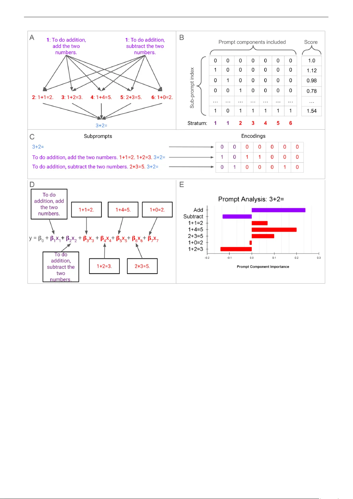
A Regr ession Framework f or Understanding Pr ompt Component Impact on LLM P erf ormance Andre w Lauziere, Jonathan Daugherty and T aisa Kushner Galois, Inc. { lauziere, jtd, taisa}@galois.com Abstract —As lar ge language models (LLMs) continue to im- pro ve and see further integration into software systems, so does the need to understand the conditions in which they will perform. W e contribute a statistical framework f or understanding the impact of specific prompt featur es on LLM perf ormance. The approach extends pr evious explainable artificial intelligence (XAI) methods specifically to inspect LLMs by fitting regression models relating portions of the prompt to LLM evaluation. W e apply our method to compare how tw o open-source models, Mistral-7B and GPT -OSS-20B, leverage the prompt to perform a simple arithmetic problem. Regression models of individual prompt portions explain 72% and 77% of variation in model performances, respectively . W e find misinformation in the form of incorrect example query-answer pairs impedes both models from solving the arithmetic query , though positive examples do not always improv e perf ormance. In terms of text-instructions, we find significant variability in the impact of positive and negative instructions – these pr ompts ha ve contradictory effects on model performance. The framework serves as a tool for decision makers in critical scenarios to gain granular insight into how the prompt influences an LLM to solve a task. Keyw ords - LLM; XAI; regression modeling; interpretable AI; prompt engineering. I . I N T RO D U C T I O N Large language models (LLMs) are a class of deep neural networks which proficiently model patterns found in text data [1]. These models have achie ved dominant performance across tasks such as text summarization [2] and machine translation [3]; their performance continues to improv e as training corpora and learning strategies such as reinforcement learning dev elop [4][5]. The models serve as the intelligence behind tools which have experienced cultural impact unseen in machine learning technology , such as Chat-GPT [6], Grammarly [7] and Micr osoft Copilot [8]. Despite comprehensiv e adoption, LLMs are some of the most opaque of machine learning methods. This is true for both intrinsic model features such as complexity due to size and inter-connecti vity , as well as extrinsic aspects including the use of large and closed-source training corpora and opti- mization routines. These factors lead to to a concerning gap between deployment of LLMs and their understanding. Larger and more powerful models are being increasingly integrated into software systems as they find new use-cases and improv e upon existing ones. Howe v er , these models are simultaneously becoming harder to understand and thus trust as they are less interpretable and more likely to be closed-source. LLMs and tools which le verage them are also highly influenced by the user-specified prompt. While guardrails imposed during fine-tuning, e.g., [5], can reduce risk, the models can still output unwanted or harmful content. This direct-access paired with a lack of understanding of the mech- anisms in which the prompt driv es LLM output compounds risk. Researchers and decision-makers alike are interested in uncov ering how LLMs function. At the moment there is little understanding as to when, why , or how an LLM will perform on a given task; researchers point to high performance on benchmark datasets as reason to trust (and thus use) their models [9][10]. In response, some researchers argue for slow- ing down AI research [11], while others pursue developing technologies to audit it. In this work, we help fill the gap in understanding how LLMs function by developing an explainable artificial intelli- gence (XAI) framework for analyzing the impact of prompt- ing on LLM performance. W e coin this framework IAMs : I nterpretable A ttribution M odel s . IAMs adapts previous XAI methods [12][13] to fit regression models comprising features representing portions of the LLM input prompt. The frame- work enables granular and statistically rigorous inspection of LLM behavior by estimating the impact of various prompt components, and combinations thereof, on model performance via regression models. Section II first introduces necessary background concerning LLMs and prompting followed by an o vervie w of XAI and a revie w of research related to this work. Then, Section III details the IAMs framework. Section IV applies IAMs to analyze and compare ho w tw o open-source LLMs solve an arithmetic problem. Finally Section V summarizes findings and outlines future work. I I . R E L A T E D W O R K LLMs are unique from other data-driven models in that they are not only trained offline (i.e., unsupervised pre-training and supervised fine-tuning) as in traditional statistical learning, but they also use “in-context learning” via the prompt to guide the model during inference [4]. As a result, the end-user has direct impact on the quality of the output, so much so that a common step of model training is to censure its ability to output harmful content [5]. Designing the prompt, or pr ompting , has become an integral part in effecti vely using an LLM. Explainable artificial intelligence (XAI) methods enable in- terpretation of lo w-bias high-v ariance machine learning mod- els; here, we focus on applying local model-agnostic methods [14] to understand LLMs by mutating the input prompt. Local methods aim to explain complex model behavior at This material is based upon work supported by the Defense Advanced Research Projects Agency (D ARP A) under Contract No. HR001124C0319. Any opinions, findings and conclusions or recommendations expressed in this material are those of the author(s) and do not necessarily reflect the views of the Defense Advanced Research Projects Agency (D ARP A). Distribution Statement “ A” (Approved for Public Release, Distribution Unlimited). 2 a specific input, whereas model-agnostic tools demonstrate interpretability independent of the complex model at hand. Ribeiro et al. dev eloped LIME: Local Interpretable Model- agnostic Explanations [12], a surrogate modeling approach which “can be applied to any classifier . ” In LIME, the local model is trained using sampled points around a specific input in the complex model space; then, a binary vector is formed representing the inclusion or e xclusion of certain features, such as words in a text model or pixels in an image model. An interpretable model is trained on the binary vectors and associated labels. The authors also propose a “fidelity- interpretability” tradeoff using an L1 regularization term (i.e., Lasso: Least Absolute Shrinkage and Selection Operator) on the local model fitting. A higher penalty will dri ve parameter estimates of less impactful features to zero. Shapley values are a canonical local model-agnostic ap- proach; the concept arises from game theory in which features of a model are “allocated payout” according to each one’ s contribution in a prediction [15]. Lundber g and Lee unified the surrogate modeling approach in LIME and Shapley values in their SHAP: Shapley Additive Explanations framework [16]. The authors show a unique set of equations for guar- anteeing Shapley value properties in an additi ve attribution model. Lundberg and Lee provide approximation algorithms for SHAP whereas both Grah and Thouvvenot [17] and Štrumbelj and Kononenko [18] provide general approximation algorithms for Shapley values. Lundberg et al. then extended SHAP to tree-based methods such as decision trees, random forests, and gradient-boosted trees [19][20]. The method was then impro ved and applied to e xplain AI models used in medicine via tree-based methods [21]. Mohammadi applied Grah and Thouvenot’ s algorithm [17] to estimate Shapley values according to a vectorization of the prompt [13]. The method assessed the extent to which certain tokens impacted LLM performance. Liu et al. also applied Shapley values to quantify which prompts best contributed to performance by considering an ensemble of prompts and iter- ativ ely pruning lower performing entries [22]. The approach used the Data Shaple y algorithm [23]. I I I . M E T H O D O L O GY Figure 1 depicts an o vervie w of IAMs applied to model ho w the prompt influences an LLM to solve an arithmetic problem. W e outline individual steps here, and then describe details of each in the following subsections. First, panel A (top left) sho ws a prompt model specifying a query of interest (blue), “3+2=, ” as well as other prompt components in six separate strata: one for task-specific text containing two choices (purple, numbered 1) and five exam- ple query-answer pairs each in an individual stratum (red, numbered 2-6). A sequence of prompt components, at most one from each stratum, forms a subpr ompt . All subprompts arising from the possible inclusion or exclusion of each prompt component are processed by a chosen LLM, and the output is ev aluated according to a user-specified score metric. Panel B (top right) shows the design matrix featuring sev en binary v ariables, one for each prompt component, signaling the inclusion (or exclusion) of each component along with the corresponding output measurement score vector . Each prompt component is referenced in bold , corresponding to a column in the design matrix (directly under the matrix). Here, the score is a function of the probability of the leading output token corresponding to the correct answer , “5. ” Scores could be binary , measuring whether or not the LLM answers a question correctly (e.g. returning “5”), or continuous (e.g. the probability of the leading token corresponding to “5”). Panel C (middle) shows how three example subprompts are encoded into binary vectors. The baseline subprompt, containing only the query of interest, is represented by an all-zero vector , as no other prompt components are used. Inclusion of at most one component from the first stratum is expressed in purple, while each example query-answer pair could be included, shown in red. The design matrix and score vector are used to fit a multiple regression model (D); visualizations allow insight into which prompt components driv e LLM performance (E). A. Pr ompt Stratification Prompt stratification casts the prompt as a series of strata, in effect sets, anchored by a query of interest, such as a request or question. W e decompose the prompt into m sets, p i , i = 1 , 2 , . . . , m . Each prompt stratum has a selection of n i = | p i | ≥ 1 possible text choices (referred to as prompt components): { p i, 1 , p i, 2 , . . . , p i,n i } , where an element p i,j is text that could be included in the prompt at location i . Each prompt stratum contains one (static) or multiple (variable) choices of text to include at that location in the prompt; the query stratum contains only the query itself. Permutations of all possible prompt components across strata yields the total subprompt set: S = p 1 × p 2 × ..., p m containing all N = Q m i =1 | p i | unique prompts. A specified LLM processes all N subprompts in S . T exts contained within a stratum are only seen one-at-a-time whereas texts between strata will co-occur . Ke y here is the fact that co-occuring prompt components can be analyzed together in regression framework. B. Encoding Pr ompts as Binary V ariables in a Regr ession F ramework Our regression framework estimates both indi vidual and joint effects of prompt components on LLM performance. Each unique subprompt contains the only component across static stratum (e.g. the query) and a subset of components across variable strata. Here, we detail steps to construct the binary design matrix from a prompt stratification such as that of Figure 1 panel A. Denote the variable stratum φ ⊂ { 1 , 2 , . . . , m } with each p l , l ∈ φ , as as a categorical variable with n l + 1 levels. Implicitly , the empty string “” is included as a baseline value in each variable stratum. A one-hot encoding maps the n l + 1 lev els to ( n l + 1) − 1 dummy v ariables, j = 1 , 2 , . . . n l . W e use the binary encodings This material is based upon work supported by the Defense Advanced Research Projects Agency (D ARP A) under Contract No. HR001124C0319. Any opinions, findings and conclusions or recommendations expressed in this material are those of the author(s) and do not necessarily reflect the views of the Defense Advanced Research Projects Agency (D ARP A). 3 Figure 1. Overview of IAMs. First in panel A, a prompt model describes texts of interest which could impact LLM performance on the query “3+2=” (blue). The first stratum (purple) contains two choices of task-specific description texts while fiv e strata (red) each have an example query-answer pair . An LLM processes and scores the full set of possible subprompts, each an input prompt containing a subset of prompt components (panel B). The inclusion (modeled with a 1) or exclusion (modeled with a 0) of components is expressed with binary variables (panel C). Pairs of encoding vectors and scores are used to fit a regression model, such as the one written in panel D. Panel E shows an example visualization of the learned model parameters conve ying importance for LLM performance. x l,j,k =    1 if component j in stratum l is acti v e in subprompt k 0 otherwise (1) across v ariable stratum l ∈ φ and lev els j = 1 , 2 , . . . , n l to estimate effects. For example, p 1 in Figure 1 panel A yields 2 dummy v ariables while each p 2 , ..., p 6 generates one dummy variable each, totaling the sev en columns in panel B. Then, interactions of dummy variables x l,j,k model the si- multaneous occurrence of multiple prompt components across variable strata. A second-order interaction dummy variable, for l ′  = l and j ′ ∈ { 1 , 2 , . . . , n l ′ } , x l,j,l ′ ,j ′ ,k =        1 if both component j in stratum l is activ e and component j ′ in stratum l ′ is activ e in subprompt k 0 otherwise (2) captures subprompts with both x l,j,k = 1 and x l ′ ,j ′ ,k = 1 ; prompt component interaction generalizes to L -order ( 2 ≤ L ≤ | φ | ) terms. Altogether , a selection of single dummy v ariables (i.e. first-order) and interaction terms (second-order , third-order , etc.) totaling M variables produces a design matrix X ∈ This material is based upon work supported by the Defense Advanced Research Projects Agency (D ARP A) under Contract No. HR001124C0319. Any opinions, findings and conclusions or recommendations expressed in this material are those of the author(s) and do not necessarily reflect the views of the Defense Advanced Research Projects Agency (D ARP A). 4 { 0 , 1 } ( nN ) × ( M +1) akin to the matrix in Panel B of Fig- ure 1. The design matrix also includes an intercept term 1 = [1 , 1 , . . . , 1] ′ ∈ R nN to estimate the score under the baseline value, i.e. when all other variables are 0. In context, this is the estimated score under the query alone with no other prompt components activ e. C. Re gr ession Modeling with Encoding V ariables Each subprompt k , represented by a ro w in the design matrix X , is processed by a chosen LLM. A user-specified scoring function ev aluates model output and produces y k . Continuous scores lead to a multiple regression approach whereas discrete (e.g. binary) output leads to a logistic regression fitting. IAMs supports continuous and binary measurements. The choice in a scoring function is limited by the LLM. Closed models only show the LLM output, as opposed to open models which rev eal internal activ ations and token probability distributions. For example, when e v aluating a closed model (e.g., GPT - 5) the scoring function could ev aluate the correctness of the output or inclusion of certain text (binary) or rate the output as in the application of LLMs-as-a-judge (continuous). On the other hand, open models such as GPT -OSS-20B can be ev aluated using all closed model scoring functions, along with scores which measure model internals. Here in our demonstration (Section IV), we le verage model openness to use a higher information score than correctness: the probability value associated with the leading token being “5. ” Broadly , continuous measurements such as R OGUE are commonly used to assess text summarization [24]; Bilingual Evaluation Understudy (BLEU) is another continuous measurement to ev aluate the accuracy of machine translation [25]. Denote y = [ y 1 , y 2 , . . . , y nN ] ′ ∈ R nN as the real-valued measured output of all processed subprompts. A multiple regression of the form y k = β 0 + X l ∈ ϕ n l X j =1 β l,j x l,j,k + e k (3) relates the binary x l,j,k variables to outputs y k via parame- ters β l,j . The intercept parameter β 0 estimates the query score, serving as a baseline. Then, error terms e k are assumed to be independent and identically distributed: N (0 , σ 2 ) . Interaction terms enable estimation of intra-stratum prompt component concurrence. Assume that two strata: l and l’ are interacted, with n l and n l ′ sub-prompts in each, respectively . Then, up to ( n l ) ∗ ( n l ′ ) interaction terms could be estimated: y k = β 0 + X l ∈ ϕ n l X j =1 β l,j x l,j,k + n l X j =1 n l ′ X j ′ =1 β l,j,l ′ ,j ′ x l,j,k x l ′ ,j ′ ,k + e k (4) Similar to LIME, we include an L1 regularization term via λ ∈ R + in the fitting to pressure coefficients corresponding to less impactful prompt components (and interactions) to zero: ˆ β λ = argmin β X l ∈ ϕ n l X j =1 nN X k =1 ( y k − ˆ y k ) 2 + λ | β | (5) Whereas the standard multiple regression optimization problem (Equation 3) has a closed-form solution, the L1- regularized least squares problem is solved via elastic-net, a coordinate descent scheme [26]. W e use the statsmodels implementation of elastic-net [27]. The case in which y ∈ { 0 , 1 } nN comes about when the output measurement function tests a property (e.g. inclusion of information or factuality) of the LLM output. Prompt stratification and design matrix follow as in the continuous output measurement case abo v e, b ut the L1-re gularized logistic regression fitting is performed via SA GA [28] implemented in scikit-learn [29]. D. F orwar d-selection Algorithm Model-selection algorithms proceed iterativ ely , adding terms from an empty model (i.e. forward-selection), removing terms from a full model (i.e backwards selection), or using a combination of both (bidirectional selection). Just as LASSO optimization (i.e. elastic-net [26]) reduces estimates without underlying context of their relationships, typical model se- lection algorithms do not assume any dependencies between variables. Howe v er , it is common practice when building interaction-term regression models to only include interaction terms if all corresponding subsets of terms are included in the model; e.g. both first-order variables in a second-order interaction term being present, and all three combinations of second-order interaction terms being present for a third-order interaction term. W e adapt a forward-selection approach to only consider the incorporation of interaction terms in which lower lev el terms are already present. The algorithm starts with an intercept term and first iterates ov er first-order components; each is only incorporated based on the estimate’ s p-value relativ e to a Bon- ferroni corrected alpha level [30]. Then, interaction terms are considered up to a maximum lev el G ov er a preselected subset of all interactions subject to increasingly higher thresholds. At each lev el g = 1 , 2 , ..., G , all interaction terms of that level among preselected strata are considered, subject to which ( g- 1 )-lev el terms are already included. E. Shapley V alue Estimation W e adjust the original Shapley value calculation [14] to handle contributions of binary variables arising from a one-hot encoding of a categorical variable. This change is a result of the mutual exclusi vity of binary variables of the same stratum; the original formula assumes any coalition of variables is fea- sible, yielding a v ariable-independent weighting of coalitions. Certain prompt components may appear in varying numbers of coalitions, depending on the prompt model at hand. Equation 6 sho ws our updated formula taking into account the varying counts of coalitions when calculating the weighted av erage of mar ginal contrib utions. W e follo w the notation of [14] though it conflicts with established IAMs notation. Here k i represents the total number of features that co- occur with prompt component i , N is the set of all prompt components, v is the scoring function, and s is a coalition This material is based upon work supported by the Defense Advanced Research Projects Agency (D ARP A) under Contract No. HR001124C0319. Any opinions, findings and conclusions or recommendations expressed in this material are those of the author(s) and do not necessarily reflect the views of the Defense Advanced Research Projects Agency (D ARP A). 5 among prompt components. In plain terms, the Shapley value of prompt component i is the av erage marginal contrib ution of the component to all prompts it could be included within. The value is a weighted av erage of all such marginal contributions. φ i ( v ) = 1 k i X s ⊂ N \{ i } ( ( k i − | s | )! | s | ! k i ! ) − 1 ( v ( s ∪{ i } ) − v ( s )) . (6) I V . C O M P A R I N G M I S T R A L - 7 B A N D G P T - O S S - 2 0 B O N A R I T H M E T I C Mistral-7B is a foundation model “engineered for ef fi- ciency”; it outperformed open-source 13B and 34B models (Llama 2, and Llama 1, respectiv ely) at time of publication across all e valuated benchmarks [31]. W e chose this model to address two core concerns: first, it enables reproducibility by being open-source and small enough to be run on con- sumer hardware; second, it showed strong performance across multiple benchmark tasks such as GSM8K [32] and MA TH [33]. W e compared Mistral-7B to GPT -OSS-20B, OpenAI’ s first open-source model since GPT -2 [34]. Though much larger than Mistral-7B, GPT -OSS-20B’ s weights were quantized; according to [34], the model can be applied to systems with “as little as 16 GB of memory . ” W e applied our regression framework to inspect how both models processed the arithmetic query “3+2=” by stratifying the prompt according to a choice of instruction texts and a set of examples. Our prompt stratification used m = 12 strata with the last stratum containing the query alone: p 12 = { “3+2=” } . W e chose to conclude each prompt with the query as Mistral- 7B is a foundation model; instruction texts and examples prior to the query were intended to guide the model to identify the token corresponding to “5” immediately after the query . The first stratum p 1 contained n 1 = 7 choices of instruction text. The underscore tok en “_” was added to measure the ef fect of “token noise” described in [35] in which tokens containing low or unrelated information impact model performance. The next three instruction texts attempt to prime the models in performing arithmetic: “Pretend you’ re a math expert.,“ “T o do addition, add the two numbers.,"’ “T o do subtraction, subtract the two numbers. ” The latter three instruction texts negate the three positi ve ones, respecti vely: “Ignore what I say ne xt., ” “T o do addition, subtract the two numbers., ” “T o do subtraction, add the two numbers. ” This initial stratum, p 1 , enables mea- surement of token noise and ho w each model improves with positiv e instruction or is robust to negati ve instruction. Then, the next 10 stratum, p 2 , ..., p 11 each contained an example- answer pair of similar arithmetic problems. The first five were all correctly answered: “0+1=1,"" “1+1=2, ” “1+2=3, ” “2+3=5, ” “1+4=5” whereas the latter fiv e were all incorr ectly answered: “1+2=4, ” “1+3=2, ” “4+3=5, ” “1+0=2, ” “2+2=3. ” The inclusion of the incorrectly answered queries enabled insight into how each model is robust to misinformation. In total, each model processed the same 8 ∗ 2 10 = 8192 unique prompts; there were eight choices in the first stratum (empty string and sev en components) and each of the ten ex- amples were either included or excluded (i.e. replaced with the empty string). W e followed [36] in using Domain Conditional Pointwise Mutual Information (DCPMI) [37]. DCPMI weights token probabilities to av oid “surface form competition, ” a phenomenon in which contextually similar tokens compete for probability mass [37]; this allowed us to process each prompt only once ( n = 1 ) using a one token generation step. First, consider the correct token probability under the null prompt, i.e. Q = “3+2=. ” This baseline probability then serves as a reference point for the correct token probabilities arising from other subprompts. Let y be an output probability distri- bution over all tokens in the vocab ulary and y c be the token corresponding to “5, ” i.e. the “correct” token. The DCPMI of y c under the “context” of the query Q when giv en the subprompt s is defined D C P M I Q ( y = y c , s ) = P ( y = y c | s ) P ( y = y c | Q ) . (7) Here, P ( y = y c | s ) is the probability an LLM estimated “5” as the first token when giv en the subprompt s , while P ( y = y c | Q ) is estimated correct token probability when given the query alone. W e followed the same fitting procedures for both Mistral- 7B and GPT -OSS-20B (henceforth, Mistral and OSS, for brevity). An initial first-order multiple regression model was fit to establish a preliminary inspection for each model. Then, two interaction-term regression model sets were fit: the first set used an L1 regularization procedure across a grid of λ v alues, while the second used our contributed forward- selection algorithm. The latter two sets of regression models contained interactions of examples, yielding insight into the marginal effects of in-context learning. A. DCPMI Distributions Before inv estigating the regression results, we observed that the correct token probability under the query (i.e. baseline) was higher in Mistral than for OSS: 0.38 and 0.22, respectively . Mistral more effectiv ely answered the query than the much larger and more recent OSS. Howe ver , we saw that the average DCPMI (i.e. the average of all correct tok en probabilities relativ e to the baseline probability) for OSS was ov er double that of Mistral, 2.36 to 1.05; this signaled that prompt com- ponents impacted OSS ov erall more positiv ely than they did for Mistral. Figure 2’ s left plot shows overlapping histograms of Mistral and OSSs’ DCPMI distributions ov er all 8192 subprompts. The unimodality of Mistral’ s distribution and bimodality of OSS also suggested that OSS responded more to prompt components than Mistral. Positi ve components led to increased DCPMI while the negati ve ones were associated with reduced DCPMI in OSS, whereas the Mistral scores were anchored by the baseline (1.0) and fell slightly on either side of the center . B. F irst-or der Regr ession Models Initial first-order multiple regression models were fit using all 17 prompt components with an intercept term. The models showed how prompt components independently related to This material is based upon work supported by the Defense Advanced Research Projects Agency (D ARP A) under Contract No. HR001124C0319. Any opinions, findings and conclusions or recommendations expressed in this material are those of the author(s) and do not necessarily reflect the views of the Defense Advanced Research Projects Agency (D ARP A). 6 Figure 2. GPT -OSS-20B was more sensitive to the prompt than Mistral-7B. Left: Mistral-7B’ s DCPMI across all 8192 subprompts (red) showed a unimodal distribution whereas GPT -OSS-20B’s DCPMI distribution was bimodal (black). The baseline DCPMI, 1.0 for both models, stands at the center of the Mistral-7B distribution. Right: Quantile-quantile (QQ) plots for Mistral (residuals in red, line of best fit in blue) and OSS (residuals in black, line of best fit in green) from first-order regression models. Overall, the unary model for OSS yielded more extreme residuals (y-axis values belo w -3 and above 3) than Mistral. The OSS residual distribution also showed deviation from normality as the tails of the distribution had less mass than expected (black dots under the green line). changes in DCPMI. First, we note the residuals in Figure 2’ s right plot compares the distributions of residuals between models. OSS residuals (black dots) deviated slightly from normality (line of best fit in green), suggesting that the first- order model did not aptly explain DCPMI variation whereas the Mistral residuals (red dots) followed closer to the line of best fit (blue). First-order models had adjusted R 2 values of 0.72 and 0.76 for Mistral and OSS, respectiv ely , which were surprisingly comparable giv en the the differences in observed DCPMI distributions. W e then validated the regression frame- work by comparing Shapley values (Equation 6) for prompt components to first-order parameter estimates, finding Pearson correlation coefficients of 0.969 and 0.997, for Mistral and OSS, respectively , indicating a strong positive relationship and validating our modeling approach. T able I compares first-order regression coefficients between Mistral and OSS. Rows are color-coded according to senti- ment: neutral in gray , positiv e or true in green, and negati ve or false in red. Asterisks correspond to p-values: *** for p < 0.0001, ** for p < 0.005, and * for p < 0.05. The “Intercept” coefficients (1.604 for Mistral and 3.324 OSS) estimated an average when all other v ariables are zero, which in context describes the baseline query DCPMI. In- cluding other prompt components via binary variables then shifted the estimated av erage. For example, when including the final prompt component “2+2=3, ” (last ro w of T able I) DCPMI lowered by 0.586 for Mistral and 0.144 for OSS, on av erage, all else constant. T o contextualize the coefficients, view each as a change in percentage from the baseline query DCPMI: 36.5% ( 1 . 604 − 0 . 586 1 . 604 = 0 . 635 ) for Mistral, and 4.3% ( 3 . 324 − 0 . 144 3 . 324 = 0 . 957 ) for OSS. Contrary to expectation, the neutral token “_” estimate had a large p-v alue for Mistral, 0.216, but a near-zero (statistically indiscernible from zero) p-value, less than 0.0001, for OSS. In context, Mistral was more robust to this the impact of this “non-sense” token than OSS, as the token estimate had a statistically significant negati ve (though small, -0.231) effect on DCPMI. This is notable as one might expect the larger , more recent model (OSS) to exhibit greater robustness than Mistral. Instruction texts showed incongruent ef fects between mod- els, while e xample query-answer pairs aligned more with a 71% Pearson correlation coefficient. Negati ve examples, in particular , hampered Mistral; e.g. “1+3=2” with estimate - 0.450, “1+2=4” with estimate -0.270. On the other hand, instruction texts “Pretend you’ re a math expert” and “Ignore what I say next” negati vely impacted OSS, with estimates - 3.057 and -2.929. Prompt components ov erall hindered both models more than guiding them, as evidenced by summing all parameter estimates for each model, although true example query-answer pairs showed statistically significant gains to DCPMI each, on av erage. T ABLE I. M I S TR A L - 7B A N D G PT- OS S - 2 0B S I MI L A R L Y U SE D E X AM P L E Q U ER Y - A N SW E R PA I RS T O S O L V E T H E Q U ER Y , B UT I N ST R UC T I O N T EX T S D E R AI L E D O S S . P RO M P T C O MP O N E NT S ( C OM P O N EN T ) A N D C O R RE S P ON D I N G FI R ST - OR D E R PAR A M E TE R E S TI M A T E S ( C O EFFI C I E NT ) F O R B OT H M IS T R A L A ND O S S E X PL A I N H OW E AC H M O D EL S O L V E D T H E QU E RY . P O S IT I V E O R T RU E C O M P ON E N T S A RE M A RK E D I N L I G H T - G RE E N B AC K GR OU N D , N E GAT IV E O R FA LS E C O MP O N E NT S A R E M A R KE D W IT H R ED BA C KG RO U N D , A N D T H E N E U TR A L U N DE R S C OR E I S M AR K E D I N G R A Y . * ** : P < 0 .0 0 0 1 , * * : P < 0 . 0 0 5, * : P < 0 . 05 . Mistral [31] OSS [34] Component Coefficient Coefficient Intercept 1.604 *** 3.324 *** _ -0.020 -0.231 *** Pretend you’ re a ... 0.045 *** -3.057 *** T o do addition, ... 0.176 *** 0.130 *** T o do subtraction, ... -0.037 ** -0.774 *** Ignore what I ... 0.069 *** -2.929 *** T o do addition, ... 0.134 *** 0.069 * T o do subtraction, ... 0.053 *** -0.144 *** 0+1=1 -0.033 *** 0.538 *** 1+1=2 0.033 *** 0.210 *** 1+2=3 0.062 *** 0.153 *** 2+3=5 0.228 *** 0.127 *** 1+4=5 0.111 *** 0.343 *** 1+2=4 -0.270 *** -0.277 *** 1+3=2 -0.450 *** -0.745 *** 4+3=5 -0.093 *** -0.085 *** 1+0=2 -0.214 *** -0.305 *** 2+2=3 -0.586 *** -0.144 *** C. Re gularized Regr ession Models W e next fit a series of regularized regression models with interactions between example query-answer pairs up to the fourth degree, totaling 393 parameters: intercept, 17 first- order terms,  10 2  = 45 second-order interactions,  10 3  = 120 third-order interactions, and  10 4  = 210 fourth-order inter- actions. Both this set of models, and the upcoming forward- selection algorithm models, in vestigated the extent to which This material is based upon work supported by the Defense Advanced Research Projects Agency (D ARP A) under Contract No. HR001124C0319. Any opinions, findings and conclusions or recommendations expressed in this material are those of the author(s) and do not necessarily reflect the views of the Defense Advanced Research Projects Agency (D ARP A). 7 multiple examples, i.e. few-shot learning, marginally impacted performance. W e performed a grid search over values of λ ∈ (0 , 0 . 003] by increments of 0.00001 to identify an optimal value λ ∗ and corresponding estimates ˆ β λ ∗ for both Mistral and OSS. The range was selected by iterativ ely halving the range from 1.0 to find the λ values which caused variation in both the magnitude of parameter estimates and MSE. Figure 3. LASSO trades off fidelity for interpretability . LASSO penalized model size (green curves, measured ∥ ˆ β λ ∥ 2 ) with increasing λ . As models shrank, performance lowered and MSE (blue curves) rose, yielding a trade-off. The grid search procedure identified an optimal λ ∗ ≈ 0 . 0004 for both models. At these “elbows” of the green curves, model reduction began to slow . Figure 3 depicts how regularization impacted the interaction-term regression models. The plot shows model capacity , measured as the L2 norm of all parameter estimates ( ∥ ˆ β λ ∥ 2 ) against model performance, measured by mean- squared error (MSE). Green curv es highlight model size (solid for Mistral, dashed for OSS) while blue curves depict MSE. The observed negati ve relationship follows from model regularization theory: constrained models are less able to capture variation and thus produce more error . Identifying the optimal λ ∗ is selected at the “elbow” of the green curves, or where model size showed resistance to regularization, about 0.0004 for both models. Compared to the unregularized fitting (i.e. λ =0), MSEs increased marginally while model sizes reduced by ≈ 40% each (approximately 3.2 to 1.8 for Mistral and 7.9 to 4.8 for OSS). The optimal parameter estimation sets, ˆ β λ ∗ , contained: 15 first-order , 37 second-order , 51 third-order , and 23 fourth-order nonzero terms in the Mistral model, and 16 first-order , 37 second-order, 70 third-order, 77 fourth-order nonzero terms in the OSS model. Selected regression models reported adjusted R-squared v alues 0.846 and 0.802, for Mistral and OSS, respectiv ely . Then, Figure 4 again shows Mistral (top) and OSS (bottom) parameter estimate norms, ∥ ˆ β λ ∥ 2 , but now stratified by order Figure 4. LASSO penalized interaction terms more than first-order terms in both Mistral and OSS. Model sizes, ∥ ˆ β λ ∥ 2 , were stratified by lev el of interaction. Blue curves show Intercept (baseline) estimates for each λ ; OSS first-order estimates remained larger than the baseline whereas all prompt component parameter estimates fell below the baseline value for Mistral, suggesting that OSS used prompt components more than Mistral, relativ e to baseline query DCPMIs. of interaction. Blue lines on each plot sho w the intercept estimate as a reference point for each level λ . A similar pattern is visible between models: lower -order terms showed stronger effects than increasingly higher order terms. Howe ver , first- order terms impacted OSS more than Mistral, relative to each set of baseline (Intercept) values. D. F orwar d-selection Models Finally , we applied our forward-selection procedure and identified a subset of the full 393-term regression model (up to fourth-order interactions among example query-answer pairs) for both Mistral and OSS starting with α = 0.05 and applying Bonferroni’ s correction at each le vel of interaction g = 1 , 2 , 3 , 4 . The resulting regressions achiev ed adjusted R-squared values of 0.861 and 0.779 using v arying prompt components and prompt component interactions. Again, the individual incorrect query-example pairs showed strong neg- ativ e ef fects on both models. Le vel-two interactions hea vily fa vored false information in both models; query-answer pairs in which at least one of the two examples was false were ov errepresented in the forward-selection models (18 of 19 in Mistral, 20 of 21 in OSS). Further , lev el-two interactions in which both examples were false tended to yield positiv e estimates, 11 of 14 in Mistral and 7 of 9 in OSS, signaling a softening ef fect of multiple pieces of misinformation. For example, in Mistral, the pairs: “1+2=4” and “1+0=2, ” “1+3=2” and “1+0=2, ” and “1+0=2” and “2+2=3” resulted in positiv e estimates: 0.261, 0.348, and 0.574. Then in OSS, the pairs: “1+3=2” and “4+3=5, ” “1+3=2” and “2+2=3, ” and “4+3=5” This material is based upon work supported by the Defense Advanced Research Projects Agency (D ARP A) under Contract No. HR001124C0319. Any opinions, findings and conclusions or recommendations expressed in this material are those of the author(s) and do not necessarily reflect the views of the Defense Advanced Research Projects Agency (D ARP A). 8 and “2+2=3” had estimates: 0.543, 0.330, and 0.346. Alto- gether , some false information disrupts both models, though decreasingly . V . C O N C L US I O N & F U T U R E W O R K IAMs provides a flexible approach to in vestigating prompt variation on LLM performance. Casting the prompt as a set of disjoint texts pa ved the way to modeling both indi vidual, and coalitions of, prompt components via established frame works such as LIME [12]. Individual and interaction regressions, regularized regression (LASSO), and our forward-selection al- gorithm jointly assist in identifying which, and to what extent, prompt components drive LLM performance. The approach was validated using an adjusted Shapley value calculation (Equation 6). W e applied the framework to inspect how the open-source models Mistral-7B and GPT -OSS-20B solved a single-digit arithmetic task, uncov ering a vulnerability to misinformation (e.g. incorrect query-answer coefficients listed in the last fi ve rows of T able I), along with strong inconsistency in ho w text- based prompts (positiv e and negati ve) impacted performance. The toy-problem was simple enough to include two relied- upon strategies of prompt design: instructing and few-shot learning. W e conclude that misinformation hampered both models more than correct information guided either, and that text-based prompts ha ve unreliable effects on model perfor- mance, often having the opposite effect one would expect. Further experimenting in tandem with previous work on few- shot learning [38]–[40] could uncover model-specific or task- specific intricacies of prompt design. Though not demonstrated, IAMs is applicable to closed- source models. Binary measurements of model output leads to a logistic regression approach; e valuations at multiple seeds giv es a sense of correctness probability per subprompt. Subsequent analyses on prompt components, coalitions, and visualizations follow from the arithmetic demonstration here. W e anticipate IAMs being especially helpful when LLMs are deployed in critical or high-risk scenarios; the framew ork will also enable granular insight into ho w in-context learning (i.e. prompting) impacts LLMs across scenarios. Furthermore, we see direct applications to e valuating and comparing AI agents. In particular, coding agents typically use a file which defines roles, personality , and other facets of the agent. Di- rectly measuring how variations in this agent blueprint driv e performance, or how agents compare on code generation more broadly , stands to improve such tools. Beyond coding agents, chatting agents which receiv e end-user ev aluation could also be compared via IAMs . In all, we belie ve the IAMs approach provides a rigorous framew ork for ev aluating the impact of prompts on model performance, filling a gap in current literature in explainable artificial intelligence. R E F E R E N C E S [1] W . X. Zhao et al., A Survey of Lar ge Language Models , arXiv:2303.18223 [cs], Mar . 2025. D O I : 10.48550/arXiv .2303. 18223 Accessed: Mar. 20, 2025. [Online]. A vailable: http : / / arxiv .org/abs/2303.18223 [2] L. Basyal and M. Sanghvi, T ext Summarization Using Lar ge Language Models: A Comparative Study of MPT-7b- instruct, F alcon-7b-instruct, and OpenAI Chat-GPT Models , arXiv:2310.10449 [cs], Oct. 2023. D O I : 10.48550/arXiv .2310. 10449 Accessed: Feb . 5, 2025. [Online]. A vailable: http : / / arxiv .org/abs/2310.10449 [3] W . Zhu et al., Multilingual Machine T ranslation with Lar ge Langua ge Models: Empirical Results and Analysis , arXiv:2304.04675 [cs], Jun. 2024. D O I : 10.48550/arXiv .2304. 04675 Accessed: Feb . 5, 2025. [Online]. A vailable: http : / / arxiv .org/abs/2304.04675 [4] T . B. Brown et al., Language Models are F ew-Shot Learners , arXiv:2005.14165 [cs], Jul. 2020. D O I : 10 .48550/ arXi v . 2005. 14165 Accessed: Sep. 20, 2023. [Online]. A vailable: http : / / arxiv .org/abs/2005.14165 [5] L. Ouyang et al., T raining language models to follow instruc- tions with human feedbac k , Mar . 2022. Accessed: Jan. 18, 2024. [Online]. A vailable: https://arxiv .org/abs/2203.02155v1 [6] ChatGPT , en-US. Accessed: Oct. 13, 2025. [Online]. A vail- able: https://chatgpt.com/ [7] F r ee AI Writing & T ext Generation T ools , en-US. Accessed: Feb . 5, 2025. [Online]. A vailable: https : / / www . grammarly . com/ai/ai- writing- tools [8] efrene, What is Micr osoft 365 Copilot? en-us. Accessed: Aug. 20, 2025. [Online]. A vailable: https : / / learn . microsoft . com / en - us / copilot / microsoft - 365 / microsoft - 365 - copilot - ov erview [9] OpenAI, GPT-4 T echnical Report , arXiv:2303.08774 [cs], Mar . 2023. Accessed: Jul. 13, 2023. [Online]. A vailable: http: //arxiv .org/abs/2303.08774 [10] G. T eam et al., Gemini: A F amily of Highly Capable Multi- modal Models , arXiv:2312.11805 [cs], May 2025. D OI : 10 . 48550 / arXi v . 2312 . 11805 Accessed: Sep. 8, 2025. [Online]. A vailable: http://arxiv .org/abs/2312.11805 [11] P ause Giant AI Experiments: An Open Letter , en-US. Ac- cessed: Aug. 25, 2025. [Online]. A vailable: https://futureoflife. org/open- letter/pause- giant- ai- e xperiments/ [12] M. T . Ribeiro, S. Singh, and C. Guestrin, "Why Should I T rust Y ou?": Explaining the Predictions of Any Classifier , arXiv:1602.04938 [cs, stat], Aug. 2016. Accessed: Jul. 25, 2024. [Online]. A vailable: http://arxiv .org/abs/1602.04938 [13] B. Mohammadi, Explaining Lar ge Language Models De- cisions Using Shapley V alues , arXiv:2404.01332 [cs], Nov . 2024. D O I : 10 . 48550 / arXi v . 2404 . 01332 Accessed: Jan. 7, 2025. [Online]. A vailable: http://arxiv .org/abs/2404.01332 [14] C. Molnar , Interpretable Machine Learning , 2nd ed. 2022. [Online]. A vailable: https://christophm .github .io/interpretable - ml- book [15] L. Shapley, “Notes on the n-Person Game – II, ” Santa Monica, Calif.: RAND Corporation, Aug. 1951. [16] S. Lundberg and S.-I. Lee, A Unified Appr oach to Interpr eting Model Pr edictions , arXiv:1705.07874 [cs, stat], Nov . 2017. Accessed: Jul. 25, 2024. [Online]. A vailable: http :// arxi v . org/ abs/1705.07874 [17] S. Grah and V . Thouvenot, “A Projected Stochastic Gradient Algorithm for Estimating Shapley V alue Applied in Attribute Importance, ” in Aug. 2020, pp. 97–115, I S B N : 978-3-030- 57320-1. D O I : 10.1007/978- 3- 030- 57321- 8_6 [18] E. Štrumbelj and I. K ononenko, “Explaining prediction models and individual predictions with feature contributions, ” Knowl- edge and Information Systems , vol. 41, no. 3, pp. 647–665, This material is based upon work supported by the Defense Advanced Research Projects Agency (D ARP A) under Contract No. HR001124C0319. Any opinions, findings and conclusions or recommendations expressed in this material are those of the author(s) and do not necessarily reflect the views of the Defense Advanced Research Projects Agency (D ARP A). 9 Dec. 2014, I S S N : 0219-3116. D O I : 10 . 1007 / s10115 - 013 - 0679 - x Accessed: Jan. 6, 2025. [Online]. A vailable: https : //doi.org/10.1007/s10115- 013- 0679- x [19] S. M. Lundberg, G. G. Erion, and S.-I. Lee, Consis- tent Individualized F eatur e Attribution for T r ee Ensembles , arXiv:1802.03888 [cs], Mar . 2019. D O I : 10.48550/arXiv .1802. 03888 Accessed: Jan. 7, 2025. [Online]. A vailable: http://arxi v . org/abs/1802.03888 [20] S. M. Lundberg et al., Explainable AI for T rees: F r om Lo- cal Explanations to Global Understanding , [cs], May 2019. D O I : 10 . 48550/ arXiv . 1905 . 04610 Accessed: Jan. 7, 2025. [Online]. A vailable: http : / / arxiv. org / abs / 1905 . 04610 [21] S. I. Amoukou, N. J.-B. Brunel, and T . Salaün, Accurate Shap- le y V alues for explaining tr ee-based models , [stat], May 2023. D O I : 10.48550/arXiv .2106.03820 Accessed: Jan. 7, 2025. [Online]. A vailable: http : / / arxiv. org / abs / 2106 . 03820 [22] H. Liu et al., Pr ompt V aluation Based on Shapley V alues , arXiv:2312.15395 [cs], Dec. 2024. D O I : 10.48550/arXiv .2312. 15395 Accessed: Feb . 5, 2025. [Online]. A vailable: http : / / arxiv .org/abs/2312.15395 [23] A. Ghorbani and J. Zou, Data Shapley: Equitable V aluation of Data for Machine Learning , arXiv:1904.02868 [stat], Jun. 2019. D OI : 10 . 48550 / arXiv . 1904 . 02868 Accessed: Feb. 5, 2025. [Online]. A vailable: http://arxiv .org/abs/1904.02868 [24] C.-Y . Lin, “ROUGE: A Package for Automatic Evaluation of Summaries, ” in T ext Summarization Branches Out , Barcelona, Spain: Association for Computational Linguistics, Jul. 2004, pp. 74–81. Accessed: Feb. 5, 2025. [Online]. A vailable: https: //aclanthology .org/W04- 1013/ [25] K. Papineni, S. Roukos, T . W ard, and W .-J. Zhu, “Bleu: A Method for Automatic Evaluation of Machine Translation, ” in Pr oceedings of the 40th Annual Meeting of the Association for Computational Linguistics , P . Isabelle, E. Charniak, and D. Lin, Eds., Philadelphia, Pennsylvania, USA: Association for Computational Linguistics, Jul. 2002, pp. 311–318. D O I : 10 .3115 /1073083 .1073135 Accessed: Feb. 5, 2025. [Online]. A vailable: https://aclanthology .org/P02- 1040/ [26] J. H. Friedman, T . Hastie, and R. T ibshirani, “Regularization Paths for Generalized Linear Models via Coordinate Descent, ” Journal of Statistical Softwar e , vol. 33, pp. 1–22, Feb . 2010, I S S N : 1548-7660. D O I : 10 . 18637 / jss . v033 . i01 Accessed: Jan. 29, 2025. [Online]. A vailable: https : / / doi . or g / 10 . 18637 / jss.v033.i01 [27] S. Seabold and J. Perktold, “Statsmodels: Econometric and statistical modeling with python, ” 2010. [28] A. Def azio, F . Bach, and S. Lacoste-Julien, SAGA: A F ast Incr emental Gradient Method W ith Support for Non-Str ongly Con vex Composite Objectives , arXi v:1407.0202 [cs], Dec. 2014. D O I : 10 . 48550 / arXiv . 1407 . 0202 Accessed: Aug. 29, 2025. [Online]. A vailable: http://arxiv .org/abs/1407.0202 [29] F . Pedre gosa et al., “Scikit-learn: Machine Learning in Python, ” Journal of Machine Learning Researc h , vol. 12, pp. 2825–2830, 2011. [30] O. J. Dunn, “Multiple Comparisons among Means, ” J ournal of the American Statistical Association , vol. 56, no. 293, pp. 52– 64, Mar . 1961, I S S N : 0162-1459, 1537-274X. D O I : 10 . 1080 / 01621459.1961.10482090 Accessed: Aug. 29, 2025. [Online]. A vailable: http : / / www . tandfonline . com / doi / abs / 10 . 1080 / 01621459.1961.10482090 [31] A. Q. Jiang et al., Mistr al 7B , arXiv:2310.06825 [cs], Oct. 2023. Accessed: Jan. 3, 2024. [Online]. A vailable: http://arxiv . org/abs/2310.06825 [32] K. Cobbe et al., T raining V erifiers to Solve Math W or d Prob- lems , arXiv:2110.14168 [cs], Nov . 2021. Accessed: Jan. 17, 2024. [Online]. A vailable: http://arxiv .org/abs/2110.14168 [33] D. Hendrycks et al., Measuring Mathematical Pr oblem Solving W ith the MA TH Dataset , arXiv:2103.03874 [cs] v ersion: 2, Nov . 2021. Accessed: Feb. 5, 2024. [Online]. A vailable: http: //arxiv .org/abs/2103.03874 [34] OpenAI et al., Gpt-oss-120b & gpt-oss-20b Model Card , arXiv:2508.10925 [cs], Aug. 2025. D O I : 10 . 48550 / arXiv . 2508 . 10925 Accessed: Aug. 27, 2025. [Online]. A vailable: http://arxiv .org/abs/2508.10925 [35] B. Mohammadi, “W ait, It’ s All T oken Noise? Always Has Been: Interpreting LLM Behavior Using Shaple y V alue, ” SSRN Electr onic Journal , 2024, I S S N : 1556-5068. D O I : 10.2139/ssrn. 4759713 Accessed: Jul. 25, 2024. [Online]. A vailable: https : //www .ssrn.com/abstract=4759713 [36] S. Seals and V . Shalin, “Evaluating the Deductiv e Competence of Large Language Models, ” in Pr oceedings of the 2024 Confer ence of the North American Chapter of the Association for Computational Linguistics: Human Language T echnologies (V olume 1: Long P apers) , K. Duh, H. Gomez, and S. Bethard, Eds., Mexico City , Mexico: Association for Computational Linguistics, Jun. 2024, pp. 8614–8630. Accessed: Jul. 25, 2024. [Online]. A vailable: https://aclanthology .org/2024.naacl- long.476 [37] A. Holtzman, P . W est, V . Shwartz, Y . Choi, and L. Zettlemoyer , “Surface Form Competition: Why the Highest Probability An- swer Isn’t Always Right, ” in Pr oceedings of the 2021 Confer- ence on Empirical Methods in Natural Language Pr ocessing , M.-F . Moens, X. Huang, L. Specia, and S. W .-t. Y ih, Eds., Online and Punta Cana, Dominican Republic: Association for Computational Linguistics, Nov . 2021, pp. 7038–7051. D O I : 10 . 18653/ v1 / 2021. emnlp - main. 564 Accessed: Jul. 25, 2024. [Online]. A vailable: https : / / aclanthology . or g / 2021 . emnlp - main.564 [38] T . Z. Zhao, E. W allace, S. Feng, D. Klein, and S. Singh, Calibrate Befor e Use: Impro ving F ew-Shot P erformance of Language Models , arXi v:2102.09690 [cs], Jun. 2021. Ac- cessed: Jan. 17, 2024. [Online]. A vailable: http : / / arxiv . or g / abs/2102.09690 [39] C.-W . Liu et al., How NOT T o Evaluate Y our Dialogue System: An Empirical Study of Unsupervised Evaluation Metrics for Dialogue Response Gener ation , arXiv:1603.08023 [cs], Jan. 2017. Accessed: Jul. 17, 2023. [Online]. A vailable: http : / / arxiv .org/abs/1603.08023 [40] H. Su et al., Selective Annotation Mak es Langua ge Models Better F ew-Shot Learners , Sep. 2022. Accessed: Jan. 18, 2024. [Online]. A vailable: https://arxiv .org/abs/2209.01975v1 This material is based upon work supported by the Defense Advanced Research Projects Agency (D ARP A) under Contract No. HR001124C0319. Any opinions, findings and conclusions or recommendations expressed in this material are those of the author(s) and do not necessarily reflect the views of the Defense Advanced Research Projects Agency (D ARP A).