When are time series predictions causal? The potential system and dynamic causal effects

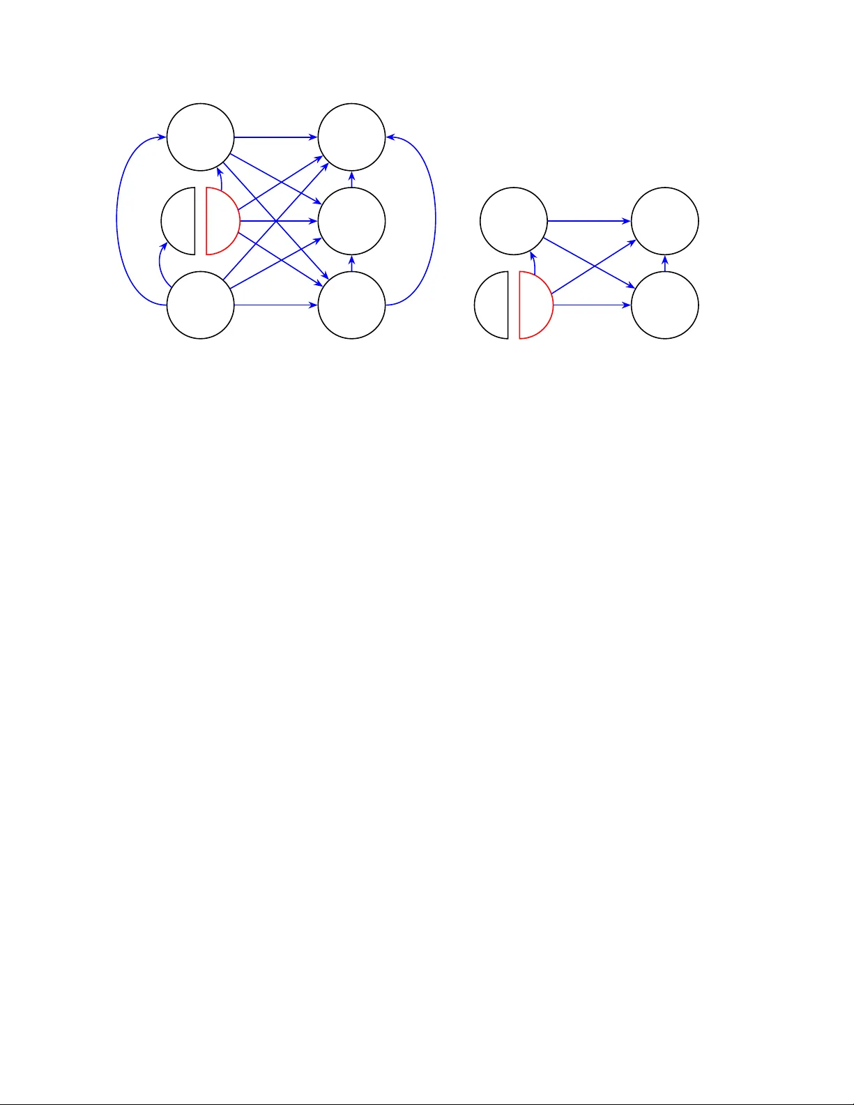
When are time series predictions causal? The p oten tial system and dynamic causal eﬀects Jacob Carlson and Neil Shephard ∗ Dep artment of Ec onomics and Dep artment of Statistics, Harvar d University, Cambridge, MA 02138, USA Marc h 24, 2026 Abstract The potential system is a nonparametric time series mo del for assessing the causal impact of mo ving an assignmen t at time t on an outcome at future time t + h , accounting for the presence of features. The p oten tial system pro vides nonparametric conten t for, e.g., time series experiments, time series regression, lo cal pro jection, impulse response functions and SV ARs. It closes a gap b etw een time series causality and nonparametric cross-sectional causal methods, and provides a foundation for man y new metho ds which ha ve causal conten t. Keyw ords: Causality , design-based inference, impulse resp onse function, potential outcomes, sequen tial assignmen t, time series. 1 In tro duction Let Y t + h b e an outcome at time t + h , where h ≥ 0 is a horizon and t is the current time, X t is a feature (whic h ma y b e, e.g., an observ ed confounder), A t is an assignment and D 1: t − 1 are past outcomes, features and assignments. When do time series data-based predictions, such as E[ Y t + h | X t , D 1: t − 1 , A t = a t ] − E[ Y t + h | X t , D 1: t − 1 , A t = a ′ t ] , measure how c hanges in the assignment at time t cause the outcomes at time t + h to mo ve? This paper pro vides suﬃcient nonparametric conditions to answer this type of question. Our approach is based on deﬁning a foundational “p oten tial system,” denoted PS . It directly connects familiar time series ob jects like impulse resp onse functions to a verage treatmen t eﬀects and, more generally , the time series causality literature to the nonparametric causal inference literature based either on p opulation or design-based inference strategies. This pap er is closely related to ﬁve time series pap ers as w ell as a stream of panel data pap ers asso ciated with James M. Robins. Bo jinov and Shephard (2019), Rambac han and Shephard (2021) and Lin and Ding (2025) w orked with a potential outcome based time series model, while Angrist ∗ W e are grateful for comments and questions from p eople attending seminars at Harv ard, MIT, Princeton, and the Universit y of Chicago. 1 and Kuersteiner (2011) and Angrist et al. (2018) deﬁne and w ork with what we call “branch p oten tial outcomes.” Both p oten tial outcomes and branc h potential outcomes app ear as a part of our PS (and hence our system could b e thought of as providing the primitiv es to these four pap ers). Bo jinov and Shephard (2019) provide man y references to the literature on dynamic causal eﬀects using potential outcome type ob jects. The v ast ma jorit y of the work in this t yp e of literature on dynamic causal eﬀects considers panel data, not pure time series, whic h is the sub ject of this pap er. The panel data literature is reviewed in, for example, Hernan and Robins (2025), Arkhangelsky and Im b ens (2024), and Chernozh uko v et al. (2023). A linear sp ecial case of the PS is a structural vector autoregression (SV AR), the workhorse of mo d- ern applied linear time series metho ds. Reviews of some of this work fo cusing on macro economics include Kilian and Lutk ep ohl (2017), F ernandez-Villav erde and Rubio-Ramirez (2010), Stock and W at- son (2018), Ramey (2016) and Jord` a and T aylor (2025). “Granger causalit y” has play ed an imp ortan t role in time series o ver the last 50 y ears. Though inspiring, Granger causality is not really ab out causality , but about prediction. (“The deﬁnition of causalit y used ab o ve is based en tirely on the predictability of some series” (Granger, 1969).) Some of the literature on Granger causalit y is discussed in, for example, Kuersteiner (2010), White and Lu (2010) and Sho jaie and F ox (2021). Harv ey and Durbin (1986) tried to assess the causal impact of a one-time assignment using a time series mo del, applying it to assess the causal impact of the in tro duction of compulsion of seat belt w earing on driver deaths in the UK. Syn thetic con trol (Abadie and Gardeazabal (2003) and Abadie et al. (2010)) is a similar idea, but enriched. There a m ultiv ariate set of outcomes mo ve together but only one is impacted b y the in terv ention. The multiv ariate data can help pin down the interv en tion under some assumed model. Abadie (2021) pro vides a review. A separate o cean of w ork on time series causality fo cuses on “control,” where an engineer builds a system which collects data to control an output in some optimal w ay to their beneﬁt. The most famous v ersion of this is linear/quadratic controller, e.g., Whittle (1982, 1983, 1990, 1996), Hansen and Sargent (2014) and Herbst and Sc horfheide (2015). Under the PS the assignments can be selected to minimize exp ected loss giv en the past data — as you would see in the con trol literature. Hence the PS bridges observ ational reduced form mo dels, exp erimen ts for time series, and control models of dynamic decision making. Muc h of the more mo dern material on con trol is phrased in terms of Mark ov decision processes (e.g., Puterman (2005)). Sometimes the researcher uses the data to learn the Mark ov decision process itself. 2 That area is usually called reinforcement learning (e.g., Sutton and Barto (2018)). The stationary Mark ov version of the PS , augmen ted with a loss function, again forms a bridge to this literature. Learning optimal dynamic treatmen t rules (or “p olicies” or “regimes”) is often phrased using p o- ten tial outcomes (e.g., Murphy (2003), Nie et al. (2021), Hec kman and Nav arro (2007), Chernozhuk ov et al. (2023), Viviano and Bradic (2026), Bradic et al. (2024)). This literature connects to our w ork in the case of sequences of interv entions, but it focuses on panel data. A notable recent exception is Kitaga wa et al. (2024), which learns optimal p olicies based on a single time series. Bo jinov et al. (2022) and Basse et al. (2023) look at “switch back designs” to optimally learn se- quences of treatmen t eﬀects from time series. There is a large other literature on sequential exp eriments whic h is not phrased in terms of p oten tial outcomes, e.g., Efron (1971) and Glynn et al. (2020), as w ell as the substan tial literature on so-called N -of-1 trials which appear prominently in, for example, the study of personalized medicine (Lillie et al. (2011)). The design-based conten t of the p oten tial system pro vides a nonparametric foundation for these settings as well. Related recent w ork includes Liang and Rech t (2025), Sc haﬀe-Odeleye et al. (2026) and Lin and Ding (2025). The latter relates potential outcomes to regression in the design-based context. Although phrased using p otential outcomes, our system can also be written using directed acyclic graph (D AG) theory , expressed using the to ols developed in the pioneering eﬀorts of Pearl (2009) and coauthors. Important related causal graph theory topics include the “Single W orld In terven tion Graph” (SWIG) asso ciated with Richardson and Robins (2013). W e use SWIG graphs to illustrate the PS and v arious constraints on the equential assignmen t mec hanism. The rest of this pap er has six sections. The p otential system and diﬀerent measures of the dynamic causal eﬀects are deﬁned in Section 2. Section 3 explores several imp ortan t examples of the PS and its relationship to v arious other common models of causalit y in the time series literature. Section 4 focuses on constrain ts on the sequential assignment mec hanism and how they allow us to iden tify diﬀeren t measures of the dynamic causal eﬀects. Section 5 considers v arious extensions of the p oten tial system, applying the framew ork to settings featuring instrumental v ariables, consecutive sequences of assignmen ts, design-based causal inference, and sto chastic dynamic programming (con trol). Section 6 concludes. There is also an Appendix containing pro ofs. Throughout, for an y (random or deterministic) sequence { x 1 , x 2 , ..., x T } w e denote for T ≥ s > t ≥ 1 the x t : s := { x t , ..., x s } , while ( A ⊥ ⊥ B ) | C denotes v ariables A and B are conditionally independent giv en C . 3 2 Deﬁning dynamic causalit y 2.1 Deﬁning the potential system The entire pap er is based on the p oten tial system, whic h we no w deﬁne. Deﬁnition 1 ( PS) . Start by deﬁning tw o sto c hastic processes. 1. The data gener ating pr o c ess , giv en b y Assumptions DGP.1 and DGP.2 . 2. The c ounterfactual pr o c ess , given b y Assumptions CP.1 and CP.2 . Assumption LP links the data generating and coun terfactual pro cesses. Applying all ﬁve assumptions deﬁnes the “p oten tial system” (denoted PS ). First, the data generating pro cess is set up using t wo assumptions. Assumption 1 ( DGP.1) . Name the data se en at time t as the split: D t :=  X T t , A T t , Y T t  T , t = 1 , ..., T . We lab el the X t ∈ X t ⊆ R d X as fe atur es; A t ∈ A t ⊆ R d A as assignments; and Y t ∈ Y t ⊆ R d Y as outc omes. F urther deﬁne D t := X t × A t × Y t , D t : s := Q s j = t D j , and A t : s := Q s j = t A j , for s ≥ t . R emark 1 (F eature in terpretation) . Dep ending on the assumptions made ab out them, features X t can pla y the role of observed confounders (explored throughout most of the paper), instrumen ts (explored in Section 5.1), or whatever else ma y b e suitable to a giv en empirical setting. ⋄ R emark 2 (F eature indexing) . The contemporaneous time indexing of features in Assumption DGP.1 is a con ven tion. F or example, features could also b e characterized b y the random v ariable X ∗ t where X t = X ∗ t − 1 . ⋄ Assumption 2 ( DGP.2) . Assume the time t assignment is gener ate d by the “se quential assignment me chanism” ( SAM ), A t = α t ( D 1: t − 1 , X t , V t ) , t = 1 , ..., T , wher e V t is crystal lize d by time t , the V t | X t , D 1: t − 1 is sto chastic and V t ⊥ ⊥ D 1: t − 1 . Thr oughout, assume the function α t := { α t ( d 1: t − 1 , x t , v t ) : d 1: t − 1 ∈ D 1: t − 1 , x t ∈ X t , v t ∈ V t } , is deterministic with r esp e ct to know le dge at time 0. 4 Second, the counterfactual pro cess is set up using tw o assumptions. Assumption 3 ( CP.1) . The time t “p otential fe atur e” and “p otential outc ome” ar e c ol le cte d as Z t ( a 1: T ) := { X t ( a 1: T ) , Y t ( a 1: T ) } , a 1: T ∈ A 1: T , X t ( a 1: T ) ∈ X t , Y t ( a 1: T ) ∈ Y t , t = 1 , ..., T , wher e a 1: T is a p ossible assignment p ath that ob eys b oth of: CP.1a (Non-anticip ation) F or al l a 1: T and a ′ 1: T ∈ A 1: T , the Z t ( a 1: T ) = Z t ( a 1: t , a ′ t +1: T ) . We write this in shorthand as Z t ( a 1: t ) . CP.1b (T riangularity) F or al l a 1: t , a ′ 1: t , the X t ( a 1: t ) = X t ( a 1: t − 1 , a ′ t ) . We write this in shorthand as X t ( a 1: t − 1 ) . Per CP.1a and CP.1b , we simplify the notation to Z t ( a 1: t ) = { X t ( a 1: t − 1 ) , Y t ( a 1: t ) } , and c ol le ct the p ath of c ounterfactuals for al l T p erio ds as Z 1: T ( a 1: T ) := { Z 1 ( a 1 ) , . . . , Z T ( a 1: T ) } . R emark 3 (Non-in terference) . Assumption CP.1a implies Z t ( a 1: T ) is realized at time t and cannot dep end on future assignments a t +1: T . This assumption rules out a time series form of what Cox (1958) generically called “interference.” The use of non-an ticipation argumen ts as important criteria for temp oral causation app ears in, for example, Granger (1980) and Rambac han and Shephard (2021). ⋄ The left-hand side of Figure 1 visualizes the counterfactual paths of p oten tial outcomes and con- founders deﬁned in CP.1 for binary assignmen ts. The righ t-hand side shows Z 1:3 corresp onding to A 1:3 = (1 , 1 , 0), highligh ting an assigned path in b old. Assumption 4 ( CP.2) . Write the “p otential br anch” at time t + h as D t,h ( a t ) := { X t,h ( a t ) , A t,h ( a t ) , Y t,h ( a t ) } , h = 0 , 1 , ..., H , a system c ounterfactual. It c orr esp onds to the assignment at time t b eing set to a t and r e c or ding the system at horizon h p erio ds later. Assume the “br anch assignment” at horizon h is A t,h ( a t ) := ( a t , h = 0 α t + h ( D 1: t − 1 , D t, 0: h − 1 ( a t ) , X t,h ( a t ) , V t + h ) , h > 0 . 5 Z 1 (1) Z 1 (0) Z 2 (1 , 1) Z 2 (1 , 0) Z 2 (0 , 1) Z 2 (0 , 0) Z 3 (1 , 1 , 1) Z 3 (1 , 1 , 0) Z 3 (1 , 0 , 1) Z 3 (1 , 0 , 0) Z 3 (0 , 1 , 1) Z 3 (0 , 1 , 0) Z 3 (0 , 0 , 0) Z 3 (0 , 0 , 1) A 1:3 = (1 , 1 , 0) Z 1 (1) Z 1 (0) Z 2 (1 , 1) Z 2 (1 , 0) Z 2 (0 , 1) Z 2 (0 , 0) Z 3 (1 , 1 , 1) Z 3 (1 , 1 , 0) Z 3 (1 , 0 , 1) Z 3 (1 , 0 , 0) Z 3 (0 , 1 , 1) Z 3 (0 , 1 , 0) Z 3 (0 , 0 , 0) Z 3 (0 , 0 , 1) Figure 1: The left ﬁgure shows all the potential outcome paths for T = 3. The righ t ﬁgure sho ws the observ ed outcome path Z 1:3 ( A 1:3 ) where A 1:3 = (1 , 1 , 0) T , indicated by the thic k blue line. The gra y arro ws indicate the missing data. Assume the “br anch p otential outc ome” and “br anch p otential fe atur e” at horizon h ar e Z t,h ( a t ) := { X t,h ( a t ) T , Y t,h ( a t ) T } T := ( { X T t , Y t ( A 1: t − 1 , a t ) T } T , h = 0 { X t + h ( A 1: t − 1 , A t, 0: h − 1 ( a t )) T , Y t + h ( A 1: t − 1 , A t, 0: h ( a t )) T } T , h > 0 . R emark 4 (Branc h p oten tial outcomes) . Deﬁnition CP.2 deﬁnes the branc h p oten tial outcomes Y t,h ( a t ). Angrist and Kuersteiner (2011) and Angrist et al. (2018) work ed directly with branc h p oten tial out- comes, without sp elling out an underlying PS . Bo jinov and Shephard (2019) work ed with p oten tial outcomes Y t + h ( a t : t + h ) assuming the assignments were sequen tially randomized and there w ere no con- founders. ⋄ The left-hand side of Figure 2 visualizes the counterfactual paths of potential branc hes, again for binary assignments. The right-hand side shows D t : t +2 corresp onding to A t = 1, highlighting the assigned path. Finally , the data generating and counterfactual pro cesses are linked by one assumption, completing the deﬁnition of the p oten tial system. Assumption 5 ( LP) . Assume Z 1: T = Z 1: T ( A 1: T ) , that is the data gener ating pr o c ess and c ounterfactual pr o c ess ar e “c onsistent.” 6 D t, 0 (1) D t, 0 (0) D t, 1 (1) D t, 1 (0) D t, 2 (1) D t, 2 (0) A t = 1 D t, 0 (1) D t, 0 (0) D t, 1 (1) D t, 1 (0) D t, 2 (1) D t, 2 (0) Figure 2: Time- t system counterfactual paths. The left ﬁgure shows all the p oten tial branches D t,h ( a t ) paths for horizon h = 0 , 1 , 2 and a t ∈ { 0 , 1 } . The right ﬁgure sho ws the observed outcome path D t : t +2 = D t, 0:2 ( A t ) where A t = 1, indicated by the thic k blue line. The gray arrows indicate the missing data. R emark 5 (“Consistency”) . Assumptions LP and CP.1 enforce “system consistency”: Z t = Z t, 0 ( A t ) = Z t ( A 1: t ). Assumption LP and Assumption CP.2 imply Z t + h = Z t,h ( A t ) for h > 0. This is the system v ersion of the “no hidden treatments” comp onen t of the Stable Unit T reatment V alue Assumption (SUTV A) formalized b y Rubin (1980); see also Robins (1986) and Imbens and Rubin (2015). ⋄ R emark 6 (Multi-perio d assignments) . Recall CP.2 mo ves the single p erio d assignment a t . Section 5.2 broadens the PS deﬁnition, replacing CP.2 with CP.2 ′ , which mov es a t : t + s , multi-perio d assignmen ts, where s ≥ 0. The rest of the system is unchanged and no new fundamen tal ideas are needed. ⋄ 2.2 Deﬁning causality with resp ect to a PS Ha ving set up the PS , it is no w p ossible to deﬁne what a dynamic causal eﬀect is and, in turn, ho w it can b e summarized in the case it is sto c hastic. Deﬁnition 2 (Dynamic causal eﬀ ects) . Assume a PS . The “dynamic causal eﬀect” is Y t,h ( a t ) − Y t,h ( a ′ t ) , the eﬀect of moving the time t assignment from a ′ t ∈ A t to a t ∈ A t on the time t + h outcome, where the horizon is h ≥ 0. W e ma y summarize the dynamic causal eﬀect in a num b er of w ays. 7 Deﬁnition 3 (Describing dynamic causal eﬀects) . Assume the PS is in L 1 . Then: 1. The “av erage treatment eﬀect” is ATE t,h ( a t , a ′ t ) := E[ { Y t,h ( a t ) − Y t,h ( a ′ t ) } ] . 2. The “conditional a verage treatment eﬀect” is CATE t,h ( a t , a ′ t ) := E[ { Y t,h ( a t ) − Y t,h ( a ′ t ) } | X t ] . 3. The “ﬁltered treatmen t eﬀect” is FTE t,h ( a t , a ′ t ) := E[ { Y t,h ( a t ) − Y t,h ( a ′ t ) } | D 1: t − 1 ] . 4. The “conditional ﬁltered treatment eﬀect” is CFTE t,h ( a t , a ′ t ) := E[ { Y t,h ( a t ) − Y t,h ( a ′ t ) } | X t , D 1: t − 1 ] . R emark 7 (T otal versus direct dynamic causal eﬀects) . The dynamic causal eﬀect at horizon one (for example) is the “total” dynamic causal eﬀect of mo ving a ′ t to a t : Y t, 1 ( a t ) − Y t, 1 ( a ′ t ) = Y t +1 ( A 1: t − 1 , a t , A t, 1 ( a t )) − Y t +1 ( A 1: t − 1 , a ′ t , A t, 1 ( a ′ t )) , whic h captures ho w moving a ′ t to a t also aﬀects future assignments. This compares to the “direct” dynamic causal eﬀect one could b e interested in, Y t +1 ( A 1: t − 1 , a t , A t +1 ) − Y t +1 ( A 1: t − 1 , a ′ t , A t +1 ) , whic h ignores how mo ving a ′ t to a t aﬀects future assignments, and is expressed directly in terms of the p oten tial outcomes (not branch p oten tial outcomes). When h = 0 the total and direct dynamic causal eﬀects are the same. ⋄ R emark 8 (Marginal dynamic causal eﬀects) . The marginal dynamic causal eﬀect, if it exists, is deﬁned as ∂ Y t,h ( a t ) ∂ a t . The av erage, conditional, ﬁltered, and conditional ﬁltered treatmen t eﬀects ha ve ob vious marginal v ersions, taking exp ectations of the marginal causal eﬀect. The simplest case is ∂ Y t, 0 ( a t ) /∂ a t = ∂ Y t ( A 1: t − 1 , a t ) /∂ a t , expressing the marginal causal eﬀect in terms of deriv ativ es of the p oten tial out- come. Results for h > 0 can b e calculated recursively . ⋄ 8 R emark 9 (Causal measures in con text) . Deﬁnition ATE t,h ( a t , a ′ t ) is t ypically called the “impulse re- sp onse function” (e.g., Sims (1980)) in time series. Av erage treatment eﬀects app ear frequen tly in, for example, randomized control trials, e.g., Imbens and Rubin (2015). Deﬁnition CATE t,h ( a t , a ′ t ) app ears frequen tly in cross-sectional observ ational causal studies, e.g., see Imbens and Rubin (2015). Deﬁnition FTE t,h ( a t , a ′ t ) is typically called the “generalized impulse resp onse function” (e.g., Koop et al. (1996)) in time series. ⋄ 3 Examples of the p otential system The follo wing are important sp ecial cases of the PS . Going forward, for notational con venience, w e deﬁne D t ( a 1: t ) := { X t ( a 1: t − 1 ) , a t , Y t ( a 1: t ) } and D 1: t ( a 1: t ) := { D 1 ( a 1 ) , ..., D t ( a 1: t ) } . 3.1 Structural equation model p oten tial systems W e b egin by discussing the nonparametric structural equation mo del (SEM) p oten tial system, a highly general example of a PS that adds useful additional structure to the p oten tial outcomes and features. Example 1 (T riangular nonparametric SEM PS ) . Assume a PS . The sequential triangular nonparamet- ric simultaneous system sets the time t p oten tial feature and p oten tial outcome as X t ( a 1: t − 1 ) = χ t ( D 1: t − 1 ( a 1: t − 1 ) , U t ) , Y t ( a 1: t ) = γ t ( D 1: t − 1 ( a 1: t − 1 ) , X t ( a 1: t − 1 ) , a t , W t ) , where all ε t := ( U T t , V T t , W T t ) T are crystallized b y time t , are indep enden t ov er time, the ε t | D 1: t − 1 are sto c hastic, the ε t ⊥ ⊥ D 1: t − 1 and the functions χ t := { χ t ( d 1: t − 1 , u t ) : d 1: t − 1 ∈ D 1: t − 1 , u t ∈ U } and γ t := { γ t ( d 1: t − 1 , x t , a t , w t ) : d 1: t − 1 ∈ D 1: t − 1 , x t ∈ X t , a t ∈ A t , w t ∈ W t } are deterministic with respect to kno wledge at time 0 for each t = 1 , ..., T . △ This mo del can be viewed as requiring that Assumption DGP.2 deﬁnes a nonparametric structural equation model (NPSEM) or structural causal mo del (SCM), formalized by P earl (1995, 2009). This framew ork for causal inference has man y direct ties to p oten tial outcomes frameworks for inference on coun terfactuals (see, e.g., Imbens (2020) or Shpitser et al. (2022) for link ages). 9 R emark 10 (Lucas critique) . Notice as a t mo ves, ( U t : T , V t : T , W t : T ) (the primitiv es whic h drive the system) do not, and the functional forms χ t , γ t in the coun terfactual process do not change (nor do es α t ). T aken together, this is a system v ersion of assuming a suﬃcien tly ric h structure to av oid the Lucas critique in economics (see, e.g., Lucas (1976), McKay and W olf (2023), Sargent (2025)). ⋄ 3.2 Linear p oten tial systems W e ma y further sp ecialize Example 1 b y incorporating linearit y , delivering the homogeneous linear Mark ov PS . Example 2 (Homogeneous linear Mark ov PS ) . Assume a PS for whic h the sequential assignmen t mec h- anism is given b y A t = α 1 D t − 1 + α 0 X t + Γ V t for conformable α 0 , α 1 , Γ and the p oten tial outcome and feature are given by X t ( a 1: t − 1 ) = χ 1 D t − 1 ( a 1: t − 1 ) + ∆ U t Y t ( a 1: t ) = γ 1 D t − 1 ( a 1: t − 1 ) + γ 0 ,X X t ( a 1: t − 1 ) + γ 0 ,A a t + Ω W t , for conformable χ 1 , ∆ , γ 0 ,X , γ 0 ,A , γ 1 , Ω, and for which { ε t } t ≥ 1 := { ( U T t , V T t , W T t ) } T t ≥ 1 ind ∼ . △ Under the mo del of Example 2, Assumption LP implies that the DGP is X t = χ 1 D t − 1 + ∆ U t , A t = α 0 X t + α 1 D t − 1 + Γ V t , Y t = γ 0 ,X X t + γ 0 ,A A t + γ 1 D t − 1 + Ω W t . W e ma y thus compactly write the DGP as a V AR(1): D t = ϕD t − 1 + B ε t where ϕ :=   χ 1 α 1 + α 0 χ 1 γ 1 + γ 0 ,X χ 1 + γ 0 ,A ( α 1 + α 0 χ 1 )   , B :=   ∆ 0 0 α 0 ∆ Γ 0 ( γ 0 ,X + γ 0 ,A α 0 )∆ γ 0 ,A Γ Ω   . W riting the system this w ay makes clear it is Mark ovian. F or the counterfactual pro cess, we start b y writing D t, 0 ( a t ) :=   X t, 0 ( a t ) A t, 0 ( a t ) Y t, 0 ( a t )   . As A t, 0 ( a t ) = a t , D t, 0 ( a t ) =   χ 1 0 γ 1 + γ 0 ,X χ 1   D t − 1 +   0 I γ 0 ,A   a t +   ∆ 0 0 0 0 0 γ 0 ,X ∆ 0 Ω   ε t , 10 and, for h = 1 , 2 , ..., H , we deﬁne D t,h ( a t ) := ϕD t,h − 1 ( a t ) + B ε t + h . The dynamic causal eﬀect on all v ariables at horizion h ≥ 0 is given by D t,h ( a t ) − D t,h ( a ′ t ) = ϕ { D t,h − 1 ( a t ) − D t,h − 1 ( a ′ t ) } = ϕ h { D t, 0 ( a t ) − D t, 0 ( a ′ t ) } = Ψ h ( a t − a ′ t ) , Ψ h := ϕ h   0 I γ 0 ,A   , whic h is non-sto chastic. Th us (abusing notation slightly) D t,h ( a t ) − D t,h ( a ′ t ) = ATE t,h ( a t , a ′ t ) = CATE t,h ( a t , a ′ t ) = FTE t,h ( a t , a ′ t ) = CFTE t,h ( a t , a ′ t ) . R emark 11 (Slutzky-F risch paradigm) . Assume the homogeneous linear Mark ov PS from Example 2. 1. If { ε t } t ≥ 1 iid ∼ , then { D t } t ≥ 1 can b e written as a V AR(1). It can also b e written as a “structural” V AR(1) — or SV AR(1) (Sims, 1980) — which is ˜ B D t = ˜ ϕD t − 1 + ε t for ˜ B := B − 1 and ˜ ϕ := B − 1 ϕ . Through recursive substitution of the V AR(1) pro cess, w e can also write the system in a “structural vector moving av erage” (SVMA) represen tation: D t + h = ϕ t + h − 1 D 1 + t + h − 2 X j =0 Θ j ε t + h − j , Θ h := ϕ h B . If the absolute v alue of the largest eigenv alue of ϕ is strictly less than one, the { ε s : s ∈ Z } is in L 2 , and the process holds inﬁnitely in the past, then D t + h = ∞ X j =0 Θ j ε t + h − j exists; this representation is often lab eled a SVMA( ∞ ) pro cess. It app ears at the heart of the so-called “Slutzky-F risch impulse-propagation paradigm” in macro economics (see, e.g., Stock and W atson (2018) for an econometric ov erview). 2. F or simplicity of exposition, consider a scalar outcome, assignmen t and feature, and let e j b e the j -th column of a 3 × 3 identit y matrix. In the Slutzky-F risch paradigm, the scalar function h 7→ e T 3 Θ h e 2 is called the impulse resp onse function (IRF) for V t (the “sho ck” to assignments, not the assignment itself ) on the outcome at horizon h , as e T 3 Θ h e 2 = E[ Y t + h | V t = 1] − E[ Y t + h | V t = 0] = e T 3 Ψ h Γ . 11 Notice further that the causal eﬀect of mo ving A t from 0 to 1 on the outcome for an y giv en h ≥ 0, the scalar function h 7→ e T 3 Ψ h (recalling that Ψ h ∈ R 3 ), can then be considered the “relative IRF”: the e T 2 Θ 0 e 2 = Γ = E[ A t | V t = 1] − E[ A t | V t = 0], and so almost surely Y t,h (1) − Y t,h (0) = e T 3 Ψ h = E[ Y t + h | V t = 1] − E[ Y t + h | V t = 0] E[ A t | V t = 1] − E[ A t | V t = 0] . This observ ation naturally extends to vector-v alued outcomes, assignments, and features. ⋄ 3.3 P oten tial systems without features Another imp ortant sp ecial case of the PS o ccurs when there are no features and the assignmen ts are in- dep enden t through time. W e ma y further specialize Example 1 to explore this setting: the Homogeneous Mark ov news impact PS . Example 3 (Homogeneous Mark ov news impact PS ) . Assume a PS . The homogeneous Mark o v news impact PS has X t ( a 1: t − 1 ) = 0 A t = V t Y t ( a 1: t ) = γ ( Y t − 1 ( a 1: t − 1 ) , a t , W t ) where { ( V t , W t ) } t ≥ 1 is an indep enden t sequence and γ is a non-random function known at time 0. △ The DGP under Example 3 is then A t = V t Y t = γ ( Y t − 1 , A t , W t ) . Note further that the h = 0 p oten tial branch and h > 0 potential branch are, respectively , Y t, 0 ( a t ) = γ ( Y t − 1 , a t , W t ) , Y t,h ( a t ) = γ ( Y t,h − 1 ( a t ) , V t + h , W t + h ) , observing that A t + h ( a t ) = V t + h for all h > 0. The causal eﬀect at h = 0 is then Y t, 0 ( a t ) − Y t, 0 ( a ′ t ) = γ ( Y t − 1 , a t , W t ) − γ ( Y t − 1 , a ′ t , W t ) and the causal eﬀect at h > 0 is Y t,h ( a t ) − Y t,h ( a ′ t ) = γ ( Y t,h − 1 ( a t ) , V t + h , W t + h ) − γ ( Y t,h − 1 ( a ′ t ) , V t + h , W t + h ) . 12 If it exists, the marginal dynamic causal eﬀect is, for h ≥ 0, ∂ Y t,h ( a t ) ∂ a t = ∂ γ ( Y t,h − 1 ( a t ) , V t + h , W t + h ) ∂ Y t,h − 1 ( a t ) ∂ Y t,h − 1 ( a t ) ∂ a t =  h Y j =1 ∂ γ ( Y t,j − 1 ( a t ) , V t + j , W t + j ) ∂ Y t,j − 1 ( a t )  ∂ Y t, 0 ( a t ) ∂ a t =  h Y j =1 ∂ γ ( Y t,j − 1 ( a t ) , V t + j , W t + j ) ∂ Y t,j − 1 ( a t )  ∂ γ ( Y t − 1 , a t , W t ) ∂ a t , whic h is typically sto c hastic. News impact causal studies appear in ﬁnancial econometrics, but are typically not expressed in causal language, and instead discuss “parameterized mec hanisms.” In that literature, a ma jor topic is understanding ho w time-v arying volatilit y of sp eculativ e assets (e.g., Bollerslev et al. (1994) and Shephard (2005)) change in resp onse to news (e.g., Campb ell and Hen tschel (1992) and Engle and Ng (1993)). A further sp ecial case of this structure is the homogeneous Marko v partially linear news impact PS , whic h sets Y t ( a 1: t ) = γ Y t − 1 ( a 1: t − 1 ) + ζ ( a t ). Then Y t = γ Y t − 1 + ζ ( V t ) , Y t, 0 ( a t ) = γ Y t − 1 + ζ ( a t ) , Y t,h ( a t ) = γ Y t,h − 1 ( a t ) + ζ ( V t + h ) for h > 0. Th us, for h ≥ 0, the dynamic causal eﬀect is non-sto c hastic with Y t,h ( a t ) − Y t,h ( a ′ t ) = γ { Y t,h − 1 ( a t ) − Y t,h − 1 ( a ′ t ) } = γ h { ζ ( a t ) − ζ ( a ′ t ) } . R emark 12 (Slutzky-F risc h paradigm, contin ued) . In macro economics, it is often assumed that as- signmen ts of interest are observ ed, indep enden t, “exogenous” sequences: assignments are “sho c ks” or “impulses.” T o explore this, return to the homogeneous linear Marko v p otential system of Example 2, no w with assignment mechanism A t = Γ V t and imp ose no features, X t ( a 1: t − 1 ) = 0 Y t ( a 1: t ) = γ 1 D t − 1 ( a 1: t − 2 ) + γ 0 ,A a t + Ω W t . The data is therefore shorter: D t = ( A T t , Y T t ) T and ε t = ( V T t , W T t ) T . Recall ε t is independent through time. The DGP is thus D t = ϕD t − 1 + B ε t where now ϕ =  0 γ 1  , B =  Γ 0 γ 0 ,A Γ Ω  . As b efore, the dynamic causal eﬀect is Ψ h ( a t − a ′ t ), though now Ψ h = ϕ h  I γ 0 ,A  13 and the IRF for assignments is Θ h e 1 = ϕ h B e 1 = ϕ h  I γ 0 ,A  Γ . If Γ = I , i.e., the assignmen t is the sho c k, then Θ h e 1 = Ψ h , and so the dynamic causal eﬀect of moving a ′ t = 0 to a t = 1 is exactly the IRF for assignments. ⋄ 3.4 m -order p oten tial systems W e ma y also consider examples of the PS that further restrict the temp oral impact of assignmen ts on p oten tial outcomes and features. Deﬁnition 4 ( m -order PS ) . Assume a PS . It is m -order causal if, for each t , A t = α t ( D t − m : t − 1 , X t , V t ) and Z t ( a 1: t − m − 1 , a t − m : t ) = Z t ( a ′ 1: t − m − 1 , a t − m : t ) , for all a 1: t , a ′ 1: t − m − 1 , m ≥ 0 . F or m -th order causal PS we write the time t potential outcome and feature using the shorthand Z t ( a t − m : t ) , burying the irrelev ance of a 1: t − m − 1 . Again, this is a t yp e of non-in terference assumption (Co x, 1958). In the imp ortan t case of Deﬁnition 4 where { ε t } = { ( U T t , V T t , W T t ) T } is a sequence of indep enden t random v ectors, then an m -order PS is m -order Mark ovian. Hence statistical methods designed for m -order Marko v processes can b e used in this setting, but now they hav e causal conten t. 3.5 PS -exogeneit y The idea of exogeneity has a long history in econometrics and is deﬁned in many diﬀeren t w ays. Some of time series literature on this topic is discussed in Engle et al. (1983). Here w e giv e a deﬁnition in the context of a PS , viewing exogeneity as a form of inv ariance with resp ect to a p ossible interv ention. That line of though t go es back at least to Simon (1953). Deﬁnition 5 ( PS -exogeneit y) . Assume a PS . An in v arian t co ordinate of Z t,h ( a t ) with respect to the in terven tion co ordinate of the a t is lab eled “ PS -exogenous” if this holds for all t and h . If all of X t,h ( a t ) is inv ariant to all of a t , then we call them “ PS -exogenous features.” 14 Example 4 (Homogeneous Mark o v linear PS with exogenous features) . Return to the homogeneous Mark ov linear PS from Example 2, but no w constrain the dynamics of the feature suc h that X t ( a 1: t − 1 ) = χ 1 X t − 1 ( a 1: t − 2 ) + ∆ U t . Then X t, 0 ( a t ) = χ 1 X t − 1 + ∆ U t , which do es not dep end up on a t . F urther, X t,h ( a t ) = χ 1 X t,h − 1 ( a t ) + ∆ U t + h , so X t,h ( a t ) is inv ariant to a t for all h . So the feature is PS -exogenous with resp ect to a t . △ PS -exogeneit y is an imp ortan t condition for extending the p otential system to applications in, e.g., design-based causal inference, discussed further in Section 5.3. Example 5 ( PS -proxy) . Sometimes researchers are interested in the causal eﬀect of assignmen ts on outcomes, but the assignmen ts themselv es are measured with error or only partially rev ealed (Stock and W atson (2018) discuss the relev ant literature and asso ciated linear metho ds). Here we provide a nonparametric version of this setup. Assume (i) a PS ; (ii) that a t splits as a t = ( a ∗ T t , ¯ a T t ) T , A t = A ∗ t × ¯ A t , a ∗ t ∈ A ∗ t , ¯ a t ∈ ¯ A t ; (iii) the en tire Z t,h ( a t ) is PS -exogenous with resp ect to ¯ a t ; (iv) write D ∗ t := ( X T t , A ∗ T t , Y T t ) T , split V t = ( V ∗ T t , ¯ V T t ) T and assume that the function α t has the triangular form A ∗ t = α ∗ t ( D ∗ 1: t − 1 , X t , V ∗ t ) , ¯ A t = ¯ α t ( D ∗ 1: t − 1 , X t , ¯ V t , A ∗ t ); (v) the ¯ D t := ( X T t , ¯ A T t , Y T t ) T is observed for t = 1 , ..., T ; (vi) A ∗ t is not directly observ ed. Then ¯ A t is a PS -pro xy for the assignment A ∗ t . An example of this is: ¯ A t = a + B A ∗ t + ¯ V t , ¯ V t ⊥ ⊥ A ∗ t , E[ ¯ V t ] = 0 , t = 1 , ..., T , where a, B are non-sto c hastic. Here all the causal conten t in this mo del is entirely driven by A ∗ t but w e only see a noisy (and p ossibly smaller or larger dimensional) version ¯ A t . △ 4 F rom predictions to causality With deﬁnitions and measures of dynamic causalit y no w in place, w e in vestigate assumptions and results that allow data-based predictions to hav e nonparametric causal interpretations. 15 4.1 Assumptions on the sequen tial assignmen t mec hanism A ma jor wa y of progressing from data-based predictions to causality is to make assumptions that constrain the b eha vior of the SAM from Assumption DGP.2 . T o do this compactly we use the notation Y t, 0: H ( A t ) = { Y t,h ( a t ) : a t ∈ A t , h = 0 , 1 , ..., H } , collecting the a t -p oten tial branch at diﬀeren t time horizons. Deﬁnition 6 (Constrain ts on the SAM ) . Assume a PS . 1. If  A t ⊥ ⊥ Y t, 0: H ( A t )  | D 1: t − 1 , X t , we sa y the SAM obeys “branc h-sequential unconfoundedness” ( SAM.BSU ). 2. If  A t ⊥ ⊥ Y t, 0: H ( A t )  | D 1: t − 1 , we sa y the SAM ob eys “branc h-sequential randomization” ( SAM.BSR ). 3. If  A t ⊥ ⊥ Y t, 0: H ( A t )  | X t , we say the SAM ob eys “branch-unconfoundedness” ( SAM.BU ). 4. If A t ⊥ ⊥ Y t, 0: H ( A t ) , we say the SAM ob eys “branch-randomization” ( SAM.BR ). Under sp ecial cases of the p oten tial system, the conditions SAM.BSU , SAM.BSR , SAM.BU and SAM.BR follo w under more primitive conditions. Theorem 1. Assume the SEM PS fr om Example 1. 1. If [ V t ⊥ ⊥ W t ] | D 1: t − 1 , X t then SAM.BSU holds. 2. If X t is D 1: t − 1 -me asur able and [ V t ⊥ ⊥ W t ] | D 1: t − 1 then SAM.BSR holds. 3. If A t = V t (assignments ar e indep endent thr ough time) and  V t ⊥ ⊥ ( D 1: t − 1 , W t )  | X t then SAM.BU holds. 4. If A t = V t (assignments ar e indep endent thr ough time) and V t ⊥ ⊥ ( D 1: t − 1 , X t , W t ) then SAM.BR holds. Pr o of. See the App endix. R emark 13 (“Exogenous” assignment noise) . By Theorem 1, using the decomp osition, w eak union, and con traction properties of conditional indep endence, and recalling that X t = χ t ( D 1: t − 1 , U t ), for SAM.BSU to hold it is suﬃcient that w e assume V t ⊥ ⊥ ( U t , W t ) | D 1: t − 1 . Similar conclusions hold for the other parts of Theorem 1 based on similar assumptions ab out the structural noise terms. ⋄ 16 R emark 14 (Indep enden t assignments) . The extra condition that { A t } t> 0 is a sequence of indep enden t random v ariables, whic h app ears for SAM.BU and SAM.BR , is certainly strong. It starred in Example 3 ab out the homogeneous Marko v news impact PS . Much of the economic time series literature measures dynamic causal quan tities through impulse response functions by assuming assignmen ts are indep endent through time. (In linear models, indep endence assumptions are often replaced b y martingale diﬀerences or w e ak white noise assumptions.) The outcome pro cess is still ﬂexible. Only the assignmen ts are highly constrained. ⋄ Assumption SAM.BSU is stated as the conditional indep endence of A t and all the elemen ts of { Y t,h ( a t ) : a t ∈ A t , h = 0 , 1 , ..., H } . A formally weak er alternative condition is to require man y pairs of conditional indep endence rather than a single v ery large join t conditional independence. This kind of pairwise assumption app ears often in cross-sectional and panel p opulation-based inference, for example Hernan and Robins (2025). W e deﬁne suc h conditions b elow. Deﬁnition 7 (P airwise constraints on the SAM ) . Assume a PS . 1. If [ A t ⊥ ⊥ Y t,h ( a t )] | ( X t , D 1: t − 1 ) for each a t ∈ A t , h = 0 , 1 , ..., H , we say the SAM ob eys SAM.BSU- . 2. If [ A t ⊥ ⊥ Y t,h ( a t )] | D 1: t − 1 for each a t ∈ A t , h = 0 , 1 , ..., H , we say the SAM ob eys SAM.BSR- . 3. If [ A t ⊥ ⊥ Y t,h ( a t )] | X t for each a t ∈ A t , h = 0 , 1 , ..., H , we say the SAM ob eys SAM.BU- . 4. If A t ⊥ ⊥ Y t,h ( a t ) for each a t ∈ A t , h = 0 , 1 , ..., H , we say the SAM ob eys SAM.BR- . Under Assumption SAM.BSU- , Figure 3 depicts the potential branc h of a PS as part of a Single W orld In terven tion T emplate (SWIT), which is a concise representation of a set of Single W orld Interv ention Graphs (SWIGs). The SWIG framew ork takes DA Gs (Directed Acyclic Graphs) as inputs and “splits” them into SWIGs at no des b eing in terv ened on, in this case at the no de that represents A t . No des do wnstream of the interv ention become potential branc hes (the Y t, 0 ( a t ) and D t,h ( a t ) for h = 0 , 1 , ..., H ). (F or other prop erties of SWIGs, see Richardson and Robins (2013).) A t a glance, Figure 3 shows that conditioning on ( X t , D 1: t − 1 ) (which are acting as observ ed confounders) mak es A t indep enden t of branch p oten tial outcomes (per standard analysis of probabilistic graphical mo dels, blo c king outgoing arro ws from ( X t , D 1: t − 1 ) separates A t from all other nodes), whic h is exactly what Assumption SAM.BSU- states. 17 Y t, 0 ( a t ) Y t, 1 ( a t ) X t X t, 1 ( a t ) A t, 1 ( a t ) D 1: t − 1 A t a t Figure 3: The PS drawn as a “Single W orld Interv ention T emplate” (SWIT), under branc h-sequential unconfoundedness — the SAM.BSU- condition. 4.2 Iden tiﬁcation of causal eﬀects through predictions Using the conditions introduced in Deﬁnition 6, the follo wing Theorem 2 shows that the causal sum- maries introduced in Deﬁnition 3 can be expressed in terms of population-based predictive quantities, deliv ering a v ersion of the promise at the start of this paper: providing conditions where the diﬀerence of tw o data-based predictions are causal at horizon h ≥ 0. Theorem 2. Always assume a PS in L 1 and set h ≥ 0 . 1. A dditional ly assume SAM.BR- , then ATE t,h ( a t , a ′ t ) = E[ Y t + h | A t = a t ] − E[ Y t + h | A t = a ′ t ] . 2. A dditional ly assume SAM.BU- , then CATE t,h ( a t , a ′ t ) = E[ Y t + h | X t , A t = a t ] − E[ Y t + h | X t , A t = a ′ t ] . 3. A dditional ly assume SAM.BSR- , then FTE t,h ( a t , a ′ t ) = E[ Y t + h | D 1: t − 1 , A t = a t ] − E[ Y t + h | D 1: t − 1 , A t = a ′ t ] . 4. A dditional ly assume SAM.BSU- , then CFTE t,h ( a t , a ′ t ) = E[ Y t + h | X t , D 1: t − 1 , A t = a t ] − E[ Y t + h | X t , D 1: t − 1 , A t = a ′ t ] . 18 Pr o of. See the App endix. Suc h predictive quan tities are not, in general, easy to estimate or approximate in practice. How ever, w e hav e made progress, mo ving from counterfactuals to observ ables which can b e modeled and predicted: w e hav e “identiﬁed” the causal ob jects deﬁned in the earlier sections. Assumption SAM.BSR- yields the SWIT in Figure 4, whic h has pruned oﬀ the confounders compared to Figure 3. The corresp onding result relating causal quan tities to data quantities under SAM.BSR- is giv en in the third part of Theorem 2. Assumption SAM.BU- yields the SWIT given in the left-hand side of Figure 5. This is the same as the SWIT for SAM.BSU- except the dependence on the history is remo ved. The corresp onding result relating causal quan tities to data quantities under SAM.BU- is giv en in the second part of Theorem 2. Assumption AM.BR- yields the SWIT for branch-randomization, sho wn on the righ t-hand side of Figure 5. Confounders no longer app ear in the graph. The corresponding result relating causal quan tities to data quantities under SAM.BR- is giv en in the ﬁrst part of Theorem 2. Y t, 0 ( a t ) Y t, 1 ( a t ) A t, 1 ( a t ) D 1: t − 1 A t a t Figure 4: The PS drawn as a “Single W orld In terven tion T emplate” (SWIT) under sequential random- ization — the SAM.BSR- case. 4.3 Linear pro jection and co v ariance stationarity W e saw in Theorem 2 v arious conditions on the PS that allow the ATE t,h ( a t , a ′ t ), CATE t,h ( a t , a ′ t ), FTE t,h ( a t , a ′ t ) and CFTE t,h ( a t , a ′ t ) to b e written as data-based (conditional) exp ectations. In some applications it is helpful to replace the data-based conditional exp ectations by pro jections. Economists often use linear pro jections (see, e.g., Angrist and Pischk e (2009)), which w e now consider in detail. Before proceeding, to establish notation, denote the usual linear pro jection of a generic random v ari- able A on 1 and a generic random v ariable B as LP[ A | 1 , B ] = κ + β B , where β = Cov( A, B )V ar( B ) − 1 19 Y t, 0 ( a t ) Y t, 1 ( a t ) X t X t, 1 ( a t ) A t, 1 ( a t ) A t a t Y t, 0 ( a t ) Y t, 1 ( a t ) A t, 1 ( a t ) A t a t Figure 5: The PS drawn as a “Single W orld In terven tion T emplate” (SWIT). Left-hand side shows the branc h unconfoundedness — the SAM.BU- case. The right-hand side shows the the branch randomization — the SAM.BR- case. and κ = E[ A ] − β E[ B ], so that ( κ, β ) = arg k,b min E A,B [( A − k − bB ) 2 ] = arg k,b min E B [(E[ A | B ] − k − bB ) 2 ] . F or this setup to mak e sense, A, B must b oth b e in L 2 and V ar( B ) > 0. Here E A,B is the expectation with resp ect to b oth A and B . E B is the exp ectation solely with resp ect to B . Assume the PS is in L 2 and work under the SAM.BR- condition, so E[ Y t + h ( a t )] = E[ Y t + h | A t = a t ] . Then the linear pro jection of Y t + h on 1, A t is LP[ Y t + h | 1 , A t = a t ] = κ t,h + β t,h a t , where β t,h = Co v( Y t + h , A t )V ar( A t ) − 1 assuming V ar( A t ) > 0. So the linear pro jection of the conditional a verage treatmen t eﬀect ATE t,h ( a t , a ′ t ) = E[ Y t + h ( a t )] − E[ Y t + h ( a ′ t )] (which is non-sto c hastic) is LP[ Y t + h | 1 , A t = a t ] − LP[ Y t + h | 1 , A t = a ′ t ] = β t,h ( a t − a ′ t ) , (whic h is non-sto chastic). R emark 15 (Linear pro jection and binary assignment) . If the PS is in L 2 and A t = { 0 , 1 } , then E[ Y t + h | A t = 1] − E[ Y t + h | A t = 0] , 20 the ATE t,h (1 , 0) under SAM.BR- , is just a diﬀerence in means, and can b e implemen ted exactly with a linear pro jection, as β t,h = Co v( Y t + h , A t )V ar( A t ) − 1 = (E[ Y t + h A t ] − E[ Y t + h ] E [ A t ]) { E[ A t ](1 − E [ A t ]) } − 1 = E[ Y t + h | A t = 1] − E[ Y t + h | A t = 0] . F urther assuming that the PS is cov ariance stationary then makes estimation easy . ⋄ R emark 16 (Linear pro jection and noisy assignment) . Recall the PS -proxy setting from Example 5, and assume that all the causal con tent in the mo del is en tirely driven b y scalar A ∗ t , but we only see a noisy v ersion ¯ A t , given by ¯ A t = a + B A ∗ t + ¯ V t , ¯ V t ⊥ ⊥ D ∗ 1: T , E[ ¯ V t ] = 0 , t = 1 , ..., T , where a, B are non-sto chastic. Notice that in this setting, the linear pro jection coeﬃcient is Co v( Y t + h , ¯ A t )V ar( ¯ A t ) − 1 = β t,h  B V ar( A ∗ t ) B 2 V ar( A ∗ t ) + V ar( ¯ V t )  . When B = 1, this recov ers the well-kno wn consequence of linear regression with classical measurement error in the regressor: attenuation bias. How ever, if B  = 1, ev en if V ar( ¯ V t ) = 0, notice that bias ma y or may not b e attenu ating, and depends on the v alue of B . ⋄ W e no w turn to a subtler case. Assume the PS is in L 2 and work under the SAM.BU- condition, so E[ Y t + h ( a t ) | X t ] = E[ Y t + h | A t = a t , X t ] . Then the linear pro jection of Y t + h on 1, A t and X t is LP[ Y t + h | 1 , A t = a t , X t ] = κ t,h + β t,h a t + δ t,h X t , where  β t,h δ t,h  = Co v( Y t + h , ( A T t , X T t ) T )  V ar( A t ) Co v( A t , X t ) Co v( X t , A t ) V ar( X t )  − 1 assuming V ar(( A T t , X T t ) T ) > 0. So the linear pro jection of the conditional av erage treatment eﬀect CATE t,h ( a t , a ′ t ) = E[ Y t + h ( a t ) | X t ] − E[ Y t + h ( a ′ t ) | X t ] (which is sto c hastic) is LP[ Y t + h | 1 , A t = a t , X t ] − LP[ Y t + h | 1 , A t = a ′ t , X t ] = β t,h ( a t − a ′ t ) (whic h is non-sto chastic, but the ﬁrst t wo moments of X t inﬂuence β t,h ). 21 Under cov ariance stationarity of { D t } , one ma y write β t,h := β h for all t . A w eaker assumption is to assume { D t } is only locally cov ariance stationary , where the dependence through time c hanges slowly (e.g., Dahlhaus (2012)). Co v ariance stationarity of { D t } is a suﬃcient condition to pro duce a time-in v arian t linear pro jected causal eﬀect, but it is not necessary . By the F risc h-W augh-Lo vell theorem (Y ule, 1907), w e ma y also write β t,h = Co v( Y t + h , A ⊥ t )V ar( A ⊥ t ) − 1 for A ⊥ t := A t − LP[ A t | 1 , X t ]. As such, w e can see it is also suﬃcien t to only require that { ( Y t , A ⊥ t ) } is cov ariance stationary to yield β t,h := β h for all t . Moreo ver, for an y random B t + h suc h that Co v( B t + h , A ⊥ t ) = 0, we hav e that β t,h = Co v( Y t + h − B t + h , A ⊥ t )V ar( A ⊥ t ) − 1 , i.e., regressing Y t + h − B t + h on A ⊥ t yields the same β t,h as regressing Y t + h on A ⊥ t . Certain choices of B t + h ma y help impro ve precision in downstream estimation, or it may b e more plausible that { ( Y t + h − B t + h , A ⊥ t ) } is cov ariance stationary . An example of this is where { Y t } is an in tegrated v ariable but { B t } is a detrender or synthetic con trol. R emark 17 (Lo cal pro jection and economics) . In the econometric time series literature the linear pro- jection approac h in the context of dynamic causal observ ational studies is asso ciated with Jord` a (2005) under the heading “local pro jection.” It is t ypically stated in the context of a cov ariance stationary time series. W ork on inferential asp ects of local pro jection includes Plagb org-Møller and W olf (2021), Olea and Plagb org-Møller (2021) and Adamek et al. (2024). ⋄ R emark 18 (Conditional linear pro jection and binary assignment) . If the PS is cov ariance stationary , is in L 2 , and A t = { 0 , 1 } , we can consider the conditional linear pro jection CLP[ Y t + h | 1 , X t ; A t = a t ] = κ ( a t ) h + β ( a t ) h X t , where β ( a t ) h = Co v(( Y t + h , X t ) | A t = a t ) { V ar( X t | A t = a t ) } − 1 and κ ( a t ) h = E[ Y t + h | A t = a t ] − β ( a t ) h E[ X t | A t = a t ], which is also quite easy to estimate. Note that CLP[ Y t + h | 1 , X t ; A t = 1] − CLP[ Y t + h | 1 , X t ; A t = 0] can then b e expressed as ( κ (1) h − κ (0) h ) + ( β (1) h − β (0) h ) X t = E[ Y t + h | A t = 1] − E[ Y t + h | A t = 0] + β (1) h ( X t − E[ X t | A t = 1]) − β (0) h ( X t − E[ X t | A t = 0]) , 22 a c onditional linear pro jection of the CATE h (1 , 0) under SAM.BU- . This conditional linear pro jection of the CATE h (1 , 0) is stochastic, just like the CATE h (1 , 0) itself, allowing for heterogeneit y in the causal eﬀect summary for diﬀerent realized v alues of X t (whic h is ruled out in the unconditional linear pro jection considered earlier). This conditional linear pro jection approach generalizes in multiple wa ys, e.g.: (i) where A t has a ﬁnite n umber of atoms, not just tw o, and (ii) computing κ ( a t ) h and β ( a t ) h b y k ernels applied to a con tinuous a t ∈ A t (though still imp osing linearity in X t ). ⋄ 4.4 Causal summaries and strict stationarity Assume throughout this subsection strict stationarity of { D t } (so the dimensions of features, assign- men ts and outcomes are time in v ariant) and the PS is in L 1 . F urther assume A t = A for all t , i.e., the assignmen t space is not c hanging ov er time. Under the condition SAM.BR- the E[ Y t + h ( a )] = E[ Y t + h | A t = a ] = µ h ( a ) , where µ h = { µ h ( a ) : a ∈ A} is a deterministic function. Thus the ATE h ( a, a ′ ) = µ h ( a ) − µ h ( a ′ ). T ypically , for strictly stationary pro cesses, µ h w ould b e estimated as a nonparametric regression of Y t + h on A t , e.g., through Nadaray a-W atson kernel regression, local linear regressions (F an and Y ao, 2005), splines, or neural netw orks. Under the weak er condition SAM.BU- the E[ Y t + h ( a ) | X t ] = E[ Y t + h | A t = a, X t ] = µ h ( a, X t ) , where µ h = { µ h ( a, x ) : a ∈ A , x ∈ X } is a deterministic function. Thus CATE h ( a, a ′ ) = µ h ( a, X t ) − µ h ( a ′ , X t ) whic h implies that, by iterated exp ectations ATE h ( a, a ′ ) = E X 1 [ µ h ( a, X 1 )] − E X 1 [ µ h ( a ′ , X 1 )] . The µ h can b e estimated by a non-parametric regression of Y t + h on A t and X t . Under the condition SAM.BSU- and imp osing the PS is m -order Marko vian (see Section 3.4), then E[ Y t + h ( a ) | X t , D t − m : t − 1 ] = E[ Y t + h | A t = a, X t , D t − m : t − 1 ] = µ h ( a, X t , D t − m : t − 1 ) , where µ h = { µ h ( a, x, d ) : a ∈ A , x ∈ X , d ∈ D m } is a deterministic function. Th us CFTE h ( a, a ′ ) = µ h ( a, X t , D t − m : t − 1 ) − µ h ( a ′ , X t , D t − m : t − 1 ) 23 whic h implies that, by iterated exp ectations ATE h ( a, a ′ ) = E X m +1 ,D 1: m [ µ h ( a, X m +1 , D 1: m )] − E X m +1 ,D 1: m [ µ h ( a ′ , X m +1 , D 1: m )] . The µ h can again b e estimated b y a non-parametric regression of Y t + h on A t , X t and D t − m : t − 1 . Under the condition SAM.BSR- plus imp osing the PS is m -order Marko vian, then E[ Y t + h ( a ) | D t − m : t − 1 ] = E[ Y t + h | A t = a, D t − m : t − 1 ] = µ h ( a, D t − m : t − 1 ) , where µ h = { µ h ( a, d ) : a ∈ A , d ∈ D m } is a deterministic function. Th us FTE h ( a, a ′ ) = µ h ( a, D t − m : t − 1 ) − µ h ( a ′ , D t − m : t − 1 ) whic h implies that, by iterated exp ectations ATE h ( a, a ′ ) = E D 1: m [ µ h ( a, D 1: m )] − E D 1: m [ µ h ( a ′ , D 1: m )] . Here µ h can b e estimated by a non-parametric regression of Y t + h on A t and D t − m : t − 1 . 4.5 Inﬂuence curves and double robustness Assume that the PS is in L 1 , that A t is made up of a ﬁnite num b er of atoms, and that SAM.BSU- holds. Deﬁne λ a t ( X t , D 1: t − 1 ) := P ( A t = a t | X t , D 1: t − 1 ), the prop ensit y score, and assume it is bounded a wa y from zero and one for all a t ∈ A t . Recall that CFTE t,h ( a t , a ′ t ) = E[ Y t + h | X t , D 1: t − 1 , A t = a t ] − E[ Y t + h | X t , D 1: t − 1 , A t = a ′ t ] . As such we hav e that ATE t,h ( a t , a ′ t ) = E[ CFTE t,h ( a t , a ′ t )] = E[E[ Y t + h | X t , D 1: t − 1 , A t = a t ]] − E[E[ Y t + h | X t , D 1: t − 1 , A t = a ′ t ]] . F rom the literature on semiparametric inference, we know that this is a classic missing data functional (Kennedy, 2024), for whic h the inﬂuence curve (or “eﬃcient inﬂuence function”) in a fully nonparametric observ ed-data mo del for ( Y t + h , A t , X t , D 1: t − 1 ) is IF ( ATE t,h ( a t , a ′ t )) = E[ Y t + h | X t , D 1: t − 1 , A t = a t ] + 1( A t = a t ) λ a t ( X t , D 1: t − 1 )  Y t + h − E[ Y t + h | X t , D 1: t − 1 , A t = a t ]  − E[ Y t + h | X t , D 1: t − 1 , A t = a ′ t ] − 1( A t = a ′ t ) λ a ′ t ( X t , D 1: t − 1 )  Y t + h − E[ Y t + h | X t , D 1: t − 1 , A t = a ′ t ]  − ATE t,h ( a t , a ′ t ) . Inﬂuence curv es are random ob jects that can b e used to construct semiparametric eﬃcient estima- tors, e.g., the doubly robust estimators that are familiar from Robins et al. (1994) and Hernan and 24 Robins (2025), or the double/debiased mac hine learning estimators familiar from Chernozh uko v et al. (2018). Semiparametric eﬃcien t inference on nonparametrically deﬁned impulse resp onse functions is explored in part in, e.g., Ballinari and W ehrli (2024), building from Ram bachan and Shephard (2021), and can b e grounded in the PS . The desirable prop erties of inﬂuence function-based estimators are dis- cussed in man y w orks (e.g., Robins et al. (1994) or Chernozh uko v et al. (2018), or see Kennedy (2024) for an ov erview). 5 Extensions 5.1 Instrumen tal v ariables and lo cal causal eﬀect summaries The PS also accommodates identiﬁcation of local summaries of causal eﬀects using instrumental v ari- ables, in the spirit of Imbens and Angrist (1994). Deﬁnition 8 (Instrumental v ariables PS ) . Assume the triangular nonparametric SEM PS from Example 1. The instrumen tal v ariables (IV) PS further assumes that χ t ( y 1: t − 1 , a 1: t − 1 , x 1: t − 1 , u t ) = χ t ( y 1: t − 1 , a 1: t − 1 , x ′ 1: t − 1 , u t ) , α t ( y 1: t − 1 , a 1: t − 1 , x 1: t − 1 , x t , v t ) = α t ( y 1: t − 1 , a 1: t − 1 , x ′ 1: t − 1 , x t , v t ) , γ t ( y 1: t − 1 , a 1: t − 1 , x 1: t − 1 , x t , a t , w t ) = γ t ( y 1: t − 1 , a 1: t − 1 , x ′ 1: t − 1 , x ′ t , a t , w t ) , for all x 1: t , x ′ 1: t ∈ X 1: t , a 1: t ∈ A 1: t , y 1: t − 1 ∈ Y 1: t − 1 , w t ∈ W t , u t ∈ U t , v t ∈ V t for all t . W e write them in shorthand as χ t ( y 1: t − 1 , a 1: t − 1 , u t ) , α t ( y 1: t − 1 , a 1: t − 1 , x t , v t ) , γ t ( y 1: t − 1 , a 1: t , w t ) . The deﬁnition of the IV PS imp oses further (exclusion) restrictions on the causal relationships of the v ariables in the PS . Under the IV PS , we ma y write X t ( a 1: t − 1 ) = χ t ( ˜ D 1: t − 1 ( a 1: t − 1 ) , U t ) , A t = α t ( ˜ D 1: t − 1 , X t , V t ) , Y t ( a 1: t ) = γ t ( ˜ D 1: t − 1 ( a 1: t − 1 ) , a t , W t ) , where ˜ D t := ( A T t , Y T t ) T and ˜ D 1: t − 1 ( a 1: t − 1 ) := { ˜ D 1 ( a 1 ) , ..., ˜ D t − 1 ( a 1: t − 1 ) } where ˜ D t ( a 1: t ) := { a t , Y t ( a 1: t ) } . Figure 6 depicts the instrumental v ariables PS in a SWIT. Under this system deﬁnition, we hav e that feature X t is a v alid instrumental variable for the time t assignmen t conditional on ˜ D 1: t − 1 , so long as (suﬃciently) the U t ⊥ ⊥ ( V t , W t ) | ˜ D 1: t − 1 and an instrumen t relev ance condition holds. By further making a monotonicity assumption familiar from Imbens and 25 Angrist (1994), letting A t = X t = { 0 , 1 } for all t , and, for all h , deﬁning A t ( x t ) := α t ( ˜ D 1: t − 1 , x t , V t ), w e can identify a lo cal summary of the causal eﬀect, E [ Y t,h (1) − Y t,h (0) | 1 { A t (1) > A t (0) } = 1 , ˜ D 1: t − 1 ] . The even t { A t (1) > A t (0) } can b e thought of as the single unit in the time series “complying” with the instrumen t. Theorem 3. Assume an instrumental variables PS wher e A t = X t = { 0 , 1 } for al l t . F urther assume: (i) [ U t ⊥ ⊥ ( V t , W t )] | ˜ D 1: t − 1 . (ii) E[ A t | X t = 1 , ˜ D 1: t − 1 ] − E[ A t | X t = 0 , ˜ D 1: t − 1 ] > 0 almost sur ely. (iii) A t (1) ≥ A t (0) almost sur ely. Then, almost sur ely, for any h = 0 , 1 , ..., H , E[ Y t,h (1) − Y t,h (0) | 1 { A t (1) > A t (0) } = 1 , ˜ D 1: t − 1 ] = E[ Y t + h | X t = 1 , ˜ D 1: t − 1 ] − E[ Y t + h | X t = 0 , ˜ D 1: t − 1 ] E[ A t | X t = 1 , ˜ D 1: t − 1 ] − E[ A t | X t = 0 , ˜ D 1: t − 1 ] . Pr o of. See the App endix. The ﬁrst condition in Theorem 3, in conjunction with the exclusion restrictions imp osed by the IV PS , grants that X t ⊥ ⊥  A t (1) , A t (0) , Y t,h (1) , Y t,h (0)  | ˜ D 1: t − 1 . The second and third conditions of Theorem 3 mirror the relev ance and monotonicit y assumptions, resp ectiv ely , in tro duced in Imbens and Angrist (1994). The empirical setting represented by the IV PS may b e relev ant to, e.g., a health system that wan ts to kno w the causal eﬀect of ingesting a drug on a patien t’s health o ver time, but can only randomly encourage the patient to do so with a text reminder; or a ride-share application company that wan ts to understand the causal eﬀect of augmen ting some asp ect of cit y-wide driv er behavior on app engagemen t, but can only pro vide that city’s driv ers with randomized incentiv es to encourage desired b eha vior at scale. 5.2 Multi-p erio d assignmen ts The same primitiv es in the PS can b e used to deﬁne p oten tial branc hes based on man y consecutive p eriods of interv ention. W e ma y call these ob jects s -p otential branches, and deﬁne them in the follo wing alternativ e to assumption CP.2 . Naturally , the 0-potential branch is a potential branch, and so p oten tial branc hes are a sp ecial case of s -p otential branc hes. 26 Y t, 0 ( a t ) Y t, 1 ( a t ) X t X t, 1 ( a t ) A t, 1 ( a t ) ˜ D 1: t − 1 A t a t Figure 6: The IV PS drawn as a “Single W orld Interv ention T emplate” (SWIT) where X t is an instru- men tal v ariable. Assumption 6 ( CP.2 ′ ) . Write the “ s -p otential br anch” for some s ≥ 0 at time t + h as D t,h ( a t : t + s ) := { X t,h ( a t : t + s ) , A t,h ( a t : t + s ) , Y t,h ( a t : t + s ) } , h = 0 , 1 , ..., H a system c ounterfactual. It c orr esp onds to the assignments at times t thr ough t + s b eing set to { a t , a t +1 , . . . , a t + s } and r e c or ding the system at horizon h p erio ds later. Assume the br anch assign- ment at horizon h is A t,h ( a t : t + s ) := ( a t + h , h ≤ s α t + h ( D 1: t − 1 , D t, 0: h − 1 ( a t : t + s ) , X t,h ( a t : t + s ) , V t + h ) , h > s. Assume the s -p otential br anch outc ome and br anch fe atur e at horizon h ar e Z t,h ( a t : t + s ) :=  X t,h ( a t : t + s ) Y t,h ( a t : t + s )  := ( { X T t , Y t ( A 1: t − 1 , a t ) T } T , h = 0 { X t + h ( A 1: t − 1 , A t, 0: h − 1 ( a t : t + s )) T , Y t + h ( A 1: t − 1 , A t, 0: h ( a t : t + s )) T } T , h > 0 . Under CP.2 ′ , analyzing dynamic causal eﬀects in the setting of Example 2, w e see that D t, 0 ( a t : t + s ) = D t, 0 ( a t ) and then recursiv ely , for h ≤ s , the D t,h ( a t : t + s ) =   X t,h ( a t : t + s ) A t,h ( a t : t + s ) Y t,h ( a t : t + s )   =   χ 1 0 γ 1 + γ 0 ,X χ 1   D t,h − 1 ( a t : t + s )+   0 I γ 0 ,A   a t + h +   ∆ 0 0 0 0 0 γ 0 ,X ∆ 0 Ω   ε t + h , while for h > s , D t,h ( a t : t + s ) = ϕD t,h − 1 ( a t : t + s ) + B ε t + h . 27 Then the dynamic causal eﬀect is again non-sto c hastic. F or h ≤ s , it is determined by the recursion D t,h ( a t : t + s ) − D t,h ( a ′ t : t + s ) =   χ 1 0 γ 1 + γ 0 ,X χ 1   { D t,h − 1 ( a t : t + s ) − D t,h − 1 ( a ′ t : t + s ) } +   0 I γ 0 ,A   ( a t + h − a ′ t + h ) and then, for h > s , D t,h ( a t : t + s ) − D t,h ( a ′ t : t + s ) = ϕ { D t,h − 1 ( a t : t + s ) − D t,h − 1 ( a ′ t : t + s ) } . 5.3 Design-based causal inference Design-based inference is extremely inﬂuen tial in randomized control trials and observ ational studies (e.g., Fisher (1925, 1935) and Imbens and Rubin (2015)). In these settings, researc hers c ho ose to condition on the p oten tial outcomes. The imp ortance of the design-based approach in panel data is highligh ted in, for example, Arkhangelsky and Imbens (2024). In time series this design-based approach was in tro duced b y Bo jinov and Shephard (2019) in their simpler setting with no features and randomized assignments. They condition on all the p oten tial outcomes Y 1: T ( A 1: T ) := { Y 1: T ( a 1: T ) : a 1: T ∈ A 1: T } , where, generically , we write Z s : t ( A 1: s − 1 , A s : t ) = { Z s : t ( A 1: s − 1 , a s : t ) : a s : t ∈ A s : t } . One of the attractions of the design-based approac h is that it allows some forms of causal inference without sp ecifying a detailed mo del for the outcomes. This is v ery comp elling, as time series has no direct form of replication. Lin and Ding (2025) further develop time series design-based studies, relating it to regression. A key ob ject of in terest in design-based causal inference is the distribution of assignments conditional on the p oten tial outcomes. This la w is naturally called the “assignmen t mec hanism,” tak en from the cross-sectional literature. Deﬁnition 9 (Assignmen t mechanism) . Assume a PS . The assignment mechanism ( AM ) is the la w of A 1: T | Z 1: T ( A 1: T ). Our goal is to sample from the AM under a particular n ull h yp othesis in order to perform design-based (causal) inference. T o wards this goal, we state the following theorem. Theorem 4. Assume the PS fr om Example 1 and that V t ⊥ ⊥ ( U t , W t , ε 1: t − 1 ) | D 1: t − 1 for al l t . Then the joint law of A 1: T , Z 1: T ( A 1: T ) , is determine d by the se quenc e Z t ( A 1: t ) | Z 1: t − 1 ( A 1: t − 1 ) and A t | [ A 1: t − 1 , Z 1: t ( A 1: t − 1 , A t )] , wher e t = 1 , ..., T . 28 Pr o of. See the App endix. Note that the join t law of A 1: T , Z 1: T ( A 1: T ) is determined b y the marginal la w of Z 1: T ( A 1: T ) and the AM . F rom Theorem 4 and the time series prediction decomp osition, the law of Z 1: T ( A 1: T ) is entirely determined by the sequence Z t ( A 1: t ) | Z 1: t − 1 ( A 1: t − 1 ), and th us the AM is solely determined by the sequence A t | [ A 1: t − 1 , Z 1: t ( A 1: t − 1 , A t )]. Notice this is close to the SAM , but diﬀers as AM additionally conditions on Y t ( A 1: t − 1 , A t ). This observ ation then motiv ates the following infeasible theorem. It uses the assumption that the features are PS -exogenous, for all t and h , whic h implies that X 1: T ( a 1: T ) = X 1: T for all a 1: T ∈ A 1: T . Theorem 5. Assume the PS fr om Example 1, that V t ⊥ ⊥ ( U t , W t , ε 1: t − 1 ) | D 1: t − 1 , that the fe atur es ar e PS -exo genous, and that for a se quenc e of assignments A ∗ 1: T the  Y t ( A ∗ 1: t − 1 , A t ) ⊥ ⊥ A ∗ t  | A ∗ 1: t − 1 , X 1: t , Y 1: t − 1 ( A ∗ 1: t − 1 ) . Then simulating A ∗ 1: T r e cursively thr ough the c onditional law A ∗ t | [ A ∗ 1: t − 1 , X 1: t , Y 1: t − 1 ( A ∗ 1: t − 1 )] , t = 1 , ..., T , (1) the r esulting A ∗ 1: T is a dr aw fr om the AM . Pr o of. See the App endix. No w the equation (1) has the same structure as the sequen tial assignment mechanism, but for the sim ulated path of the assignmen t. How ever, the la w of (1) is still infeasible to sample from as the Y 1: t − 1 ( A ∗ 1: t − 1 ) are counterfactuals w e do not see: we only see the outcomes Y 1: t − 1 = Y 1: t − 1 ( A 1: t − 1 ). T o mak e sampling feasible, we deﬁne the null comp osite hypothesis H 0 : Y t ( a 1: t ) = Y t ( a ′ 1: t ) + g t ( a 1: t , a ′ 1: t ; θ ) , ∀ a 1: t , a ′ 1: t ∈ A 1: t , t = 1 , ..., T , where g t is a deterministic, kno wn, parameterized function where θ ∈ Θ. Under the null, the Y t ( A ∗ 1: t ) = Y t + g t ( A ∗ 1: t , A 1: t ; θ ) , t = 1 , ..., T . Hence in the setting of Example 1, with the features being PS -exogenous, knowledge of the SAM allows sim ulating A ∗ 1: T from the AM under the null. Example 6 (Homogeneous, linear causal eﬀects) . Assume a PS , the features are PS -exogenous and imp ose a parametric null h yp othesis that g t ( a 1: t , a ′ 1: t ) = Q X j =0 ψ j ( a t − j − a ′ t − j ) + P X j =1 ϑ j g t − j ( a 1: t − j , a ′ 1: t − j ) , a 1: t , a ′ 1: t ∈ A 1: t , t > Q ≥ 0 , P ≥ 0 , 29 so the causal eﬀect is homogeneous and linear in contemporaneous and past assignments with parameters θ = ( ψ T 0: Q , ϑ T 1: P ) T . When θ = 0 then this is the time series Fisher-type sharp null of no causal eﬀect used b y Bo jinov and Shephard (2019), but now extended to the case of features and causal dynamics. △ The adv antage of this design-based approach is that, for an y v alue of θ , we can sim ulate under the n ull B copies of the triple D ∗ 1: T = { X T 1: T , A ∗ T 1: T , Y 1: T ( A ∗ 1: T ) T } T , whic h can then b e compared to the actual data D 1: T . The comparison is made through a lo w dimensional statistic T ( D ∗ 1: T ) designed b y the researcher, comparing it to T ( D 1: T ): rejecting the null if T ( D 1: T ) is large compared to the B simulated versions of T ( D ∗ 1: T ). Consequently we can ﬁnd an exact conﬁdence region C for θ (and so in turn causal eﬀects) b y in verting the distribution of the test, so that P ( θ ∈ C ) = 1 − α, where α ∈ (0 , 1) is selected b y the researcher. A signiﬁcant virtue of this approach is that w e are parametrically mo deling the causal eﬀects, but are en tirely agnostic ab out the underlying dynamics of the outcomes. A downside is that it requires the ability to sim ulate from SAM through (1), the law of A ∗ t | [ A ∗ 1: t − 1 , X 1: t , { Y 1: t − 1 = y 1: t − 1 + g 1: t − 1 ( A ∗ 1: t − 1 , A 1: t − 1 ) } ] . F or exp erimen tal data this should b e kno wn. F or observ ational data, the SAM can b e estimated from the data, using Assumption CP.2 to extrap olate from the assignments based on lagged observ ables (that is Assumption DGP.2 ) to assignmen ts based on lagged counterfactuals. In the imp ortan t sp ecial case of the news impact PS this diﬃculty en tirely disapp ears as A t is an i.i.d. sequence. Example 7. Suppose there are no confounders, the PS is Mark o vian, the assignments are binary and under the null hypothesis the causal eﬀects follo w Example 6 with Q = 1 and P = 0. Then a t ∈ { 0 , 1 } , while p ∗ t ( a t ) := P ( A ∗ t = a t | A ∗ t − 1 , Y t − 1 ( A ∗ t − 2: t − 1 )) , Y t ( a 1: t ) = Y t + ψ 0 ( a t − A t ) + ψ 1 ( a t − 1 − A t − 1 ) , so θ = ψ 0:1 . If p ∗ t = { p ∗ t ( a ) : a ∈ { 0 , 1 }} is kno wn, this allows us to calculate Y 1: T ( A ∗ 1: T ) and thus sim ulate the entire path A ∗ 1: T , Y 1: T ( A ∗ 1: T ) , 30 with the inputs θ , Y 1: T and A 1: T . Deﬁne the inv erse probabilit y w eighted test statistic T ( A ∗ 1: t ) := 1( A ∗ t = 1) Y t ( A ∗ 1: t − 1 , 1) p ∗ t (1) − 1( A ∗ t = 0) Y t ( A ∗ 1: t − 1 , 0) p ∗ t (0) . Then E[ T ( A ∗ 1: t ) | Y 1: T ( A 1: T ) , A ∗ 1: t − 1 ] = Y t ( A ∗ 1: t − 1 , 1) − Y t ( A ∗ 1: t − 1 , 0) = ψ 0 . W e compare the observed T ( A 1: t ) with B indep enden t simulated (under θ ) v ersions. △ Example 8. Assume a news impact PS with A t = V t , Y t ( a 1: t ) = ξ t + f ( a 1: t ) , where (i) V t is i.i.d.; (ii) ξ t is strictly stationary in L 1 ; (iii) V t ⊥ ⊥ ξ t ; and (iv) f is a deterministic function. Then the assumption SAM.BR holds. This implies that E[ Y t,h ( a )] = E[ Y t + h | A t = a ] . Assume that assignments are binary for all t , and deﬁne the statistic b T = T ( A 1: T , Y 1: T ) = W     b E[ Y t | A t = 1] − b E[ Y t | A t = 0] b E[ Y t +1 | A t = 1] − b E[ Y t +1 | A t = 0] b E[ Y t + H | A t = 1] − b E[ Y t + H | A t = 0]     , where W is some conformable, non-stochastic weigh t matrix and ˆ E[ · | · ] is an appro ximation of the conditional expectation. If the assignments are binary , these estimated conditional exp ectations are just diﬀerences in means; otherwise, E[ Y t + h | A t = a ] may be estimated using, e.g., a kernel regression. T ypically W will b e a selection matrix, fo cusing on a single lead. T o carry out inference w e condition on all the p oten tial outcomes. W e assume the comp osite null h yp othesis and that the causal eﬀects follow Example 6 with P = 0 and Q = H . Note that under the n ull Y t,h (1) − Y t,h (0) = E[ Y t,h (1)] − E[ Y t,h (0)] = ψ h almost surely . Letting Y ∗ 1: T := Y 1: T ( A ∗ 1: T ), under the n ull h yp othesized θ , for b = 1 , ..., B , simulate A ∗ ( b ) 1: T , Y ∗ ( b ) 1: T and T ∗ b := T ( A ∗ ( b ) 1: T , Y ∗ ( b ) 1: T ) , and compute, for example, if T is a scalar, L ∗ b := b T − T ∗ b . F or a 95% test, we reject the null based on n ull hypothesized θ if 0 / ∈ [ Q L ∗ (0 . 025) , Q L ∗ (0 . 975)] 31 for Q L ∗ the quantile function for L ∗ . W e estimate the quantiles b y the sample quan tiles from the sim ulated L ∗ 1 , ..., L ∗ B . A 95% CI for θ are all the v alues of θ ∈ Θ for whic h the asso ciated n ull is not rejected. △ 5.4 Sto c hastic dynamic programming There is a large literature on control, e.g., Anderson and Mo ore (1979), Whittle (1981, 1982, 1996), Bertsek as (1987) and Hansen and Sargen t (2014). Here, the discussion will connect the control literature to the potential system, using the abov e notation, but with no features. Often the control literature is collected under the label of sto c hastic dynamic programming. Deﬁne the sequence which w ould minimize exp ected future loss J t from taking actions a t : T ∈ A t : T as b a t : T | t − 1 := arg min a t : T ∈A t : T E[ J t ( A 1: t − 1 , a t : T ) | D 1: t − 1 ] , t ∈ { 1 , 2 , ..., T } , giv e information at time t − 1. Then tak e the time-t assignment as A t = b a t | t − 1 , t = 1 , ..., T , ignoring the other b a t +1: T | t − 1 . Recall that the p oten tial system’s “consistency” means that D t = D t ( A 1: t ) = D t ( A 1: t − 1 , b a t | t − 1 ) . Here, the A t is previsible — it is sto c hastic but en tirely dependent on past outcome data. Thus the SAM is probabilistically degenerate. The time t “v alue” is deﬁned as V t := E  J t ( A 1: t − 1 , b a t : T | t − 1 ) | D 1: t − 1  = min a t : T ∈A t : T E[ J t ( A 1: t − 1 , a t : T ) | D 1: t − 1 ] , the b est p ossible exp ected future loss, giv en past data. In stochastic dynamic programming, the se- quence  b a t | t − 1  is typically called the control sequence, as it is assumed to b e under the con trol of the researc her. Under the PS , it determines the SAM . The causal eﬀect of moving the assignment to a t , a wa y from the optimal v alue a ′ t = A t = b a t | t − 1 , is particularly interesting. The immediate dynamic causal eﬀect on the outcome is Y t, 0 ( a t ) − Y t, 0 ( a ′ t ) = Y t ( A 1: t − 1 , a t ) − Y t whic h spills ov er to the eﬀect at horizon h = 1, Y t, 1 ( a t ) − Y t, 1 ( a ′ t ) = Y t +1 ( A 1: t − 1 , a t , A t, 1 ( a t )) − Y t +1 , 32 where A t, 1 ( a t ) = b a t +1 | t ( a t ) with b a t +1: T | t ( a t ) := arg min a t +1: T ∈A t +1: T E[ J t ( A 1: t − 1 , a t , a t +1: T ) | D 1: t − 1 , D t, 0 ( a t )] b eing the optimal assignmen t path from time t +1 to time T thinking we had seen the data D 1: t − 1 , D t, 0 ( a t ). In the control con text, the researcher typically assumes losses are time separable, that is J t ( A 1: t − 1 , a t : T ) = T +1 X j = t L j ( A 1: t − 1 , a t : j ) , L t ( a 1: t ) = ℓ t ( Y t − 1 ( a 1: t − 1 ) , a t ) , where the ℓ t = { ℓ t ( y , a ) : y ∈ Y , a ∈ A} are kno wn deterministic functions for all t = 1 , ..., T , and in the ﬁnal perio d for all a, a ′ ∈ A , the ℓ T +1 ( y , a ) = ℓ T +1 ( y , a ′ ) := ℓ T +1 ( y ). Hence L t ( a 1: t ) is random only b ecause of the p otential outcome, while L t + h ( A 1: t − 1 , a t : t + h ) is random b ecause of the assignmen t sequence and the potential outcome. Lo oking forw ard from time t to time T , the o verall loss for a sequence of future assignments a t : T sums up future individual p eriod losses. This can b e written as a bac kward recursion J t ( A 1: t − 1 , a t : T ) = L t ( A 1: t − 1 , a t ) + J t +1 ( A 1: t − 1 , a t , a t +1: T ) . This recursive structure sets the stage for deﬁning and solving Bellman equations. 6 Conclusion This pap er deﬁnes and works on the p oten tial system ( PS ), a foundational nonparametric model for studying how an assignmen t at time t causally aﬀects an outcome at time t + h , p ossibly in the presence of confounders. It yields familiar measures of causalit y — explored through examples connected to v arious other literatures in time series causality — that can be mapped to data-based predictions under familiar assumptions from cross-sectional causal inference. Because this foundational mo del is deﬁned in terms of low-lev el nonparametric primitives, it can b e readily extended to numerous other time series causalit y settings, such as design-based based inference, the study of more exotic causal eﬀects, control, and b eyond. This paper do es not discuss the intricate details of estimation nor inference — our focus is on iden tiﬁcation. Plagborg-Møller and Kolesar (2025) and Ballinari and W ehrli (2024) are p opulation- based inference pap ers which can sit on top of our PS , giving them causal meaning, cov ering inference for the relationship b et ween what w e call the branch p oten tial outcomes and the assignmen ts. This builds oﬀ inference results in Ram bachan and Shephard (2021). Other recent work on non-linear impulse resp onse functions include Goncalves et al. (2021, 2024) and Gourieroux and Lee (2023). 33 References Abadie, A. (2021). Synthetic control: feasibilit y , data requiremen ts and metho dological asp ects. Journal of Ec onomics Liter atur e 59 , 391–425. Abadie, A., A. Diamond, and J. Hainmueller (2010). Synthetic control metho ds for comparative case studies: Estimating the eﬀect of California’s tobacco con trol program. Journal of the Americ an Statistic al Asso ciation 105 , 493–505. Abadie, A. and J. Gardeazabal (2003). The economic costs of conﬂict: A case study of the basque coun try . Americ an Ec onomic R eview 93 , 113–132. Adamek, R., S. Smeek es, and I. Wilms (2024). Lo cal pro jection inference in high dimensions. Ec ono- metrics Journal 27 , 323–342. Anderson, B. D. O. and J. B. Mo ore (1979). Optimal Filtering . Englew o o d Cliﬀs: Prentice-Hall. Angrist, J. D., ` O. Jord` a, and G. M. Kuersteiner (2018). Semiparametric estimates of monetary p olicy eﬀects: string theory revisited. Journal of Business & Ec onomic Statistics 36 , 371–387. Angrist, J. D. and G. M. Kuersteiner (2011). Causal eﬀects of monetary sho cks: Semiparametric condi- tional indep endence tests with a multinomial propensity score. R eview of Ec onomics and Statistics 93 , 725–747. Angrist, J. D. and J.-S. Pischk e (2009). Mostly Harmless Ec onometrics: A n Empiricist’s Comp anion . Princeton: Princeton Univ eristy Press. Arkhangelsky , D. and G. Im b ens (2024). Causal mo dels for longitudinal and panel data. Ec onometrics Journal 27 , C1–C61. Ballinari, D. and A. W ehrli (2024). Semiparametric inference for impulse resp onse functions using double/debiased machine learning. Unpublished pap er: Swiss National Bank. Basse, G., Y. Ding, and P . T oulis (2023). Minimax designs for causal eﬀects in temp oral exp erimen ts with treatment habituation. Biometrika 110 , 155–168. Bertsek as, D. (1987). Dynamic Pr o gr amming: Deterministic and Sto chastic Mo dels . Englew o od Cliﬀs, New Jersey: Pren tice-Hall. Bo jinov, I. and N. Shephard (2019). Time series exp eriments and causal estimands: exact randomization tests and trading. Journal of the Americ an Statistic al Asso ciation 114 , 1665–1682. Bo jinov, I., D. Simchi-Levi, and J. Zhao (2022). Design and analysis of switch back exp erimen ts. Man- agement Scienc e 69 , 3759–3777. Bollerslev, T., R. F. Engle, and D. B. Nelson (1994). ARCH mo dels. In R. F. Engle and D. McF adden (Eds.), The Handb o ok of Ec onometrics, V olume 4 , pp. 2959–3038. Amsterdam: North-Holland. Bradic, J., W. Ji, and Y. Zhang (2024). High-dimensional inference for dynamic treatment eﬀects. The A nnals of Statistics 52 , 415–440. Campb ell, J. Y. and L. Hen tschel (1992). No news is go o d news: an asymmetric mo del of changing v olatility in stock returns. Journal of Financial Ec onomics 31 , 281–318. Chernozh uko v, V., D. Chetverik o v, M. Demirer, E. Duﬂo, C. Hansen, W. Newey , and J. Robins (2018). Double/debiased machine learning for treatmen t and structural parameters. The Ec onometrics Jour- nal 21 , C1–C68. Chernozh uko v, V., W. Newey , R. Singh, and V. Syrgk anis (2023). Automatic Debiased Machine Learn- ing for Dynamic T reatment Eﬀects and General Nested F unctionals. arXiv:2203.13887 [econ]. 34 Co x, D. R. (1958). Planning of Exp eriments . Oxford: Wiley . Dahlhaus, R. (2012). Lo cally stationary pro cesses. In T. Subba Rao, S. Subba Rao, and C. Rao (Eds.), Handb o ok of Statistics: V olume 30 , pp. 351–413. Elsevier. Efron, B. (1971). F orcing a sequential exp erimen t to b e balanced. Biometrika 58 , 403–417. Engle, R. F., D. F. Hendry , and J. F. Ric hard (1983). Exogeneity . Ec onometric a 51 , 277–304. Engle, R. F. and V. Ng (1993). Measuring and testing the impact of news on volatilit y . Journal of Financ e 48 , 1749–1778. F an, J. and Q. Y ao (2005). Nonline ar Time Series . New Y ork: Springer. F ernandez-Villav erde, J. and J. Rubio-Ramirez (2010). Structural vector autoregressions. In S. Durlauf and L. E. Blume (Eds.), Macr o e c onometrics and Time Series Analysis, The New Palgr ave Ec onomics Col le ction , pp. 303–307. London: Palgra ve Macmillan. Fisher, R. A. (1925). Statistic al Metho ds for R ese ar ch Workers (1 ed.). London: Oliver and Bo yd. Fisher, R. A. (1935). Design of Exp eriments (1 ed.). London: Oliv er and Bo yd. Glynn, P . W., R. Johari, and M. Rasouli (2020). Adaptive experimental design with temp oral in ter- ference: A maxim um lik eliho od approac h. A dvanc es in Neur al Information Pr o c essing Systems 33 , 15054–15064. Goncalv es, S., A. M. Herrera, L. Kilian, and E. Pesa ven to (2021). Impulse resp onse analysis for struc- tural dynamic mo dels with nonlinear regressors. Journal of Ec onometrics 225 , 107–130. Goncalv es, S., A. M. Herrera, L. Kilian, and E. P esav ento (2024). State-dependent local pro jections. Journal of Ec onometrics 244 , 105702. Gourieroux, C. and Q. Lee (2023). Nonlinear impulse resp onse functions and lo cal pro jections. Unpub- lished pap er, Department of Economics, Universit y of T oronto. Granger, C. W. J. (1969). In vestigating causal relations b y econometric mo dels and cross-sp ectral metho ds. Ec onometric a 37 , 424–438. Granger, C. W. J. (1980). T esting for causalit y: a p ersonal viewpoint. Journal of Ec onomic Dynamics and Contr ol 2 , 329–352. Hansen, L. P . and T. J. Sargent (2014). R e cursive Mo dels of Dynamic Line ar Ec onomies . Princeton: Princeton Universit y Press. Harv ey , A. C. and J. Durbin (1986). The eﬀects of seat belt legislation on British road casualties: A case study in structural time series modelling. Journal of the R oyal Statistic al So ciety, Series A 149 , 187–227. Hec kman, J. J. and S. Nav arro (2007). Dynamic discrete c hoice and dynamic treatmen t eﬀects. Journal of Ec onometrics 136 , 341–396. Herbst, E. and F. Schorfheide (2015). Bayesian Estimation of DSGE Mo dels . Princeton: Princeton Univ ersity Press. Hernan, M. A. and J. M. Robins (2025). Causal Infer enc e . Bo ca Raton: Chapman & Hall. F orthcoming. Im b ens, G. and D. B. Rubin (2015). Causal Infer enc e for Statistics, So cial and Biome dic al Scienc es: A n Intr o duction . Cambridge Univ ersity Press. Im b ens, G. W. (2020). Poten tial outcome and directed acyclic graph approac hes to causalit y: Relev ance for empirical practice in economics. Journal of Ec onomic Liter atur e 58 , 1129–1179. 35 Im b ens, G. W. and J. D. Angrist (1994). Identiﬁcation and estimation of local a verage treatment eﬀects. Ec onometric a 62 , 467–475. Jord` a, ` O. (2005). Estimation and inference of impulse responses b y local pro jections. Americ an Ec o- nomic R eview 95 , 161–182. Jord` a, ` O. and A. M. T aylor (2025). Lo cal pro jections. Journal of Ec onomic Liter atur e 63 , 59–110. Kennedy , E. H. (2024). Semiparametric doubly robust targeted double mac hine learning: A review. In E. Lab er, B. Chakrab ort y , E. E. M. Mo odie, T. Cai, and M. V. D. Laan (Eds.), Handb o ok of Statistic al Metho ds for Pr e cision Me dicine , pp. 207–236. Bo ca Raton: Chapman and Hall/CRC. Kilian, L. and H. Lutkepohl (2017). Structur al V e ctor Autor e gr essive A nalysis . Cam bridge: Cambridge Univ ersity Press. Kitaga wa, T., W. W ang, and M. Xu (2024). P olicy choice in time series by empirical w elfare maximiza- tion. Unpublished paper: Departmen t of Economics, Bro wn Universit y . Ko op, G., M. H. P esaran, and S. M. P otter (1996). Impulse resp onse analysis in nonlinear m ultiv ariate mo dels. Journal of Ec onometrics 74 , 119–147. Kuersteiner, G. (2010). Granger-Sims causalit y . In S. N. Durlauf and L. Blume (Eds.), Macr o e c onomics and Time Series A nalysis , pp. 119–134. Palgra ve Macmillian. Liang, T. and B. Rech t (2025). Randomization inference when N equals one. Biometrika 112 . Lillie, E. O., B. P atay , J. Diaman t, B. Issell, E. T op ol, and N. J. Schork (2011). The n-of-1 clinical trial: the ultimate strategy for individualizing medicine? Personalize d Me dicine 8 , 161–173. Lin, Z. and P . Ding (2025). Unifying regression-based and design-based causal inference in time-series exp erimen ts. Unpublished paper: Departmen t of Statistics, U.C. Berkeley . Lucas, R. E. (1976). Econometric p olicy ev aluation: A critique. Carne gie-R o chester Confer enc e Series on Public Policy 1 , 19–46. McKa y , A. and C. K. W olf (2023). What can time-series regressions tell us ab out p olicy coun terfactuals? Ec onometric a 91 , 1695–1725. Murph y , S. A. (2003). Optimal dynamic treatment regimes. Journal of the R oyal Statistic al So ciety, Series B 65 , 331–366. Nie, X., E. Brunskill, and S. W ager (2021). Learning when-to-treat policies. Journal of the A meric an Statistic al Asso ciation 116 , 392–409. Olea, J. L. M. and M. Plagb org-Møller (2021). Lo cal pro jection inference is simpler and more robust than you think. Ec onometric a 89 , 1789–1823. P earl, J. (1995). Causal diagrams for empirical researc h. Biometrika 82 , 669–688. P earl, J. (2009). Causality: Mo dels, R esasoning and Infer enc e (2 ed.). Cambridge Universit y Press. Plagb org-Møller, M. and M. Kolesar (2025). Dynamic causal eﬀects in a nonlinear world: the go od, the bad, and the ugly (with discussion). Journal of Business and Ec onomic Statistics 43 , 737–754. Plagb org-Møller, M. and C. K. W olf (2021). Local pro jections and V ARs estimate the same impulse rep onse functions. Ec onometric a 89 , 955–980. Puterman, M. (2005). Markov De cision Pr o c esses: Discr ete Sto chastic Dynamic Pr o gr amming . Hobo- k en, New Jersey: Wiley . 36 Ram bachan, A. and N. Shephard (2021). When do common time series estimands hav e nonparametric causal meaning? Unpublished pap er: Departmen t of Economics, Harv ard Universit y . Ramey , V. A. (2016). Macro economic sho c ks and their propagation. In J. B. T aylor and H. Uhlig (Eds.), Handb o ok of Macr o e c onomics , V olume 2A, Chapter 2, pp. 71–162. North-Holland. Ric hardson, T. S. and J. M. Robins (2013). Single world interv en tion graphs (SWIGs): A uniﬁcation of the counterfactual and graphical approaches to causality . Center for the Statistics and the So cial Scienc es, University of Washington Series. Working Pap er 128 , 2013. Robins, J. M. (1986). A new approac h to causal inference in mortalit y studies with sustained exp osure p eriods: Application to con trol of the healthy w orker surviv or eﬀect. Mathematic al Mo del ling 7 , 1393–1512. Robins, J. M., A. Rotnitzky , and L. P . Zhao (1994). Estimation of regression co eﬃcien ts when some regressors are not alw ays observed. Journal of the Americ an Statistic al Asso ciation 89 , 846–866. Rubin, D. B. (1980). Randomization analysis of exp erimen tal data: The Fisher randomization test commen t. Journal of the Americ an Statistic al Asso ciation 75 , 591–593. Sargen t, T. J. (2025). Macro economics after Lucas. Journal of Politic al Ec onomy 133 , 3390–3417. Sc haﬀe-Odeleye, T., K. T ak anashi, V. Karwa, E. M. Airoldi, and K. McAlinn (2026). Dynamic causal inference with time series data. Unpublished: Departmen t of Statistical Science, F ox School of Business, T emple Univ ersity . Shephard, N. (2005). Sto chastic V olatility: Sele cte d R e adings . Oxford: Oxford Univ ersity Press. Sho jaie, A. and E. B. F o x (2021). Granger causalit y: A review and recent adv ances. A nnual R eview of Statistics and its Applic ation 9 , 289–319. Shpitser, I., T. S. Ric hardson, and J. M. Robins (2022). Multiv ariate Counterfactual Systems and Causal Graphical Mo dels. In H. Geﬀner, R. Dec hter, and J. Y. Halp ern (Eds.), Pr ob abilistic and Causal Infer enc e (1 ed.)., pp. 813–852. New Y ork, NY, USA: A CM. Simon, H. A. (1953). Causal ordering and iden tiﬁability . In W. C. Ho od and T. C. Koopmans (Eds.), Studies in Ec onometric Metho d: Cow les Commission Mono gr aph , pp. 49–74. New Y ork: Wiley . Sims, C. A. (1980). Macro economics and realit y. Ec onometric a 48 , 1–48. Sto c k, J. H. and M. W. W atson (2018). Iden tiﬁcation and estimation of dynamic causal eﬀects in macro economics. Ec onomic Journal 128 , 917–948. Sutton, R. S. and A. G. Barto (2018). R einfor c ement L e arning: An Intr o duction (2 ed.). Bradford Bo oks. Viviano, D. and J. Bradic (2026). Dynamic cov ariate balancing: estimating treatment eﬀects o ver time with p otential local pro jections. Biometrika . F orthcoming. White, H. and X. Lu (2010). Granger causality and dynamic structural systems. Journal of Financial Ec onometrics 8 , 193–243. Whittle, P . (1981). Risk-sensitive linear/quadratic/Gaussian control. A dvanc es in Applie d Pr ob abil- ity 13 , 764–777. Whittle, P . (1982). Optimisation over Time , V olume 1. Chichester: Wiley . Whittle, P . (1983). Optimisation over Time , V olume 2. Chichester: Wiley . Whittle, P . (1990). Risk-sensitive Optimal Contr ol . Chichester: Wiley . 37 Whittle, P . (1996). Optimal Contr ol; Basics and Beyond . Chichester: Wiley . Y ule, G. U. (1907). On the theory of correlation for an y n umber of v ariables, treated b y a new system of notation. Pr o c e e dings of the R oyal So ciety of L ondon. Series A, Containing Pap ers of a Mathematic al and Physic al Char acter 79 , 182–193. 38 7 App endix 7.1 Pro ofs Theorem 1. Assume the SEM PS fr om Example 1. 1. If [ V t ⊥ ⊥ W t ] | D 1: t − 1 , X t then SAM.BSU holds. 2. If X t is D 1: t − 1 -me asur able and [ V t ⊥ ⊥ W t ] | D 1: t − 1 then SAM.BSR holds. 3. If A t = V t (assignments ar e indep endent thr ough time) and  V t ⊥ ⊥ ( D 1: t − 1 , W t )  | X t then SAM.BU holds. 4. If A t = V t (assignments ar e indep endent thr ough time) and V t ⊥ ⊥ ( D 1: t − 1 , X t , W t ) then SAM.BR holds. Pr o of. Note that, by the recursion of Example 1, an y Y t,h ( a t ) for h = 1 , ..., H only dep ends on v ariation in, for any a t , D 1: t − 1 , X t , W t , { ε t + h } h ≥ s ≥ 1 and for h = 0 depends only on D 1: t − 1 , X t , W t , . T o satisfy condition SAM.BSU , it suﬃces that  ( D 1: t − 1 , X t , V t ) ⊥ ⊥ ( D 1: t − 1 , X t , W t , { ε t + s } h ≥ s ≥ 1 )  | D 1: t − 1 , X t whic h reduces to the condition that  V t ⊥ ⊥ ( W t , { ε t + s } h ≥ s ≥ 1 )  | D 1: t − 1 , X t . Tw o conditions that imply this condition, using the contraction prop ert y of conditional independence, are V t ⊥ ⊥ W t | D 1: t − 1 , X t , V t ⊥ ⊥ { ε t + s } h ≥ s ≥ 1 | D 1: t − 1 , X t , W t . Ho wev er, this second condition is implied b y (using the weak union property and recalling that X t = χ t ( D 1: t − 1 , U t )) { ε t + s } h ≥ s ≥ 1 ⊥ ⊥ ( ε t , D 1: t − 1 ) whic h is indeed true by the join t indep endence of the ε t across all time. As such, assuming the ﬁrst prop ert y completes the proof. T o satisfy SAM.BSR it suﬃces that  ( D 1: t − 1 , X t , V t ) ⊥ ⊥ ( D 1: t − 1 , X t , W t , { ε t + s } h ≥ s ≥ 1 )  | D 1: t − 1 39 whic h reduces to the condition that ( X t , V t ) ⊥ ⊥ ( X t , W t , { ε t + s } h ≥ s ≥ 1 ) | D 1: t − 1 . By assuming that X t is D 1: t − 1 -measurable, we only require that V t ⊥ ⊥ ( W t , { ε t + s } h ≥ s ≥ 1 ) | D 1: t − 1 . This condition similarly follo ws from the tw o other conditions (using the con traction property) [ V t ⊥ ⊥ W t ] | D 1: t − 1 , V t ⊥ ⊥ { ε t + s } h ≥ s ≥ 1 | W t , D 1: t − 1 . The conclusion of this part of the theorem is then immediate using the same argumen ts as for the ﬁrst part of the theorem. If A t = V t then to satisfy SAM.BU it suﬃces that  V t ⊥ ⊥ ( D 1: t − 1 , X t , W t , { ε t + s } h ≥ s ≥ 1 )  | X t whic h reduces to the condition that  V t ⊥ ⊥ ( D 1: t − 1 , W t , { ε t + s } h ≥ s ≥ 1 )  | X t . By contraction, this condition is implied b y the conditions  V t ⊥ ⊥ ( D 1: t − 1 , W t )  | X t ,  V t ⊥ ⊥ { ε t + s } h ≥ s ≥ 1  | X t , D 1: t − 1 , W t . The second condition is once again gran ted using the same argumen t as for the ﬁrst part of the theorem pro of, and we assume the other. If A t = V t then to satisfy SAM.BR it suﬃces that  V t ⊥ ⊥ ( D 1: t − 1 , X t , W t , { ε t + s } h ≥ s ≥ 1 )  . By contraction, this condition is implied b y the conditions V t ⊥ ⊥ ( D 1: t − 1 , X t , W t ) , V t ⊥ ⊥ { ε t + s } h ≥ s ≥ 1 | ( D 1: t − 1 , X t , W t ) . The second condition is once again gran ted using the same argument as for the ﬁrst part of the the theorem pro of, and we assume the other. Theorem 2. Always assume a PS in L 1 and set h ≥ 0 . 40 1. A dditional ly assume SAM.BR- , then ATE t,h ( a t , a ′ t ) = E[ Y t + h | A t = a t ] − E[ Y t + h | A t = a ′ t ] . 2. A dditional ly assume SAM.BU- , then CATE t,h ( a t , a ′ t ) = E[ Y t + h | X t , A t = a t ] − E[ Y t + h | X t , A t = a ′ t ] . 3. A dditional ly assume SAM.BSR- , then FTE t,h ( a t , a ′ t ) = E[ Y t + h | D 1: t − 1 , A t = a t ] − E[ Y t + h | D 1: t − 1 , A t = a ′ t ] . 4. A dditional ly assume SAM.BSU- , then CFTE t,h ( a t , a ′ t ) = E[ Y t + h | X t , D 1: t − 1 , A t = a t ] − E[ Y t + h | X t , D 1: t − 1 , A t = a ′ t ] . Pr o of. W e start with the CFTE t,h ( a t , a ′ t ) case. Deﬁne the regression function µ a t t,h ( X t , D 1: t − 1 ) := E[ Y t + h | A t = a t , X t , D 1: t − 1 ] . Then note that for any a t ∈ A t µ a t t,h ( X t , D 1: t − 1 ) = E[ Y t + h | A t = a t , X t , D 1: t − 1 ] = E[ Y t,h ( a t ) | A t = a t , X t , D 1: t − 1 ] ( PS ) = E[ Y t,h ( a t ) | X t , D 1: t − 1 ] . ( SAM.BSU- ) It is then clear that for any a t , a ′ t ∈ A t CFTE t,h ( a t , a ′ t ) = µ a t t,h ( X t , D 1: t − 1 ) − µ a ′ t t,h ( X t , D 1: t − 1 ) . The corresponding pro ofs for FTE t,h ( a t , a ′ t ), ATE t,h ( a t , a ′ t ), and CATE t,h ( a t , a ′ t ) are immediate based on this deriv ation, follo wing an identical structure. Theorem 3. Assume an instrumental variables PS wher e A t = X t = { 0 , 1 } for al l t . F urther assume: (i) [ U t ⊥ ⊥ ( V t , W t )] | ˜ D 1: t − 1 . (ii) E[ A t | X t = 1 , ˜ D 1: t − 1 ] − E[ A t | X t = 0 , ˜ D 1: t − 1 ] > 0 almost sur ely. (iii) A t (1) ≥ A t (0) almost sur ely. 41 Then, almost sur ely, for any h = 0 , 1 , ..., H , E[ Y t,h (1) − Y t,h (0) | 1 { A t (1) > A t (0) } = 1 , ˜ D 1: t − 1 ] = E[ Y t + h | X t = 1 , ˜ D 1: t − 1 ] − E[ Y t + h | X t = 0 , ˜ D 1: t − 1 ] E[ A t | X t = 1 , ˜ D 1: t − 1 ] − E[ A t | X t = 0 , ˜ D 1: t − 1 ] . Pr o of. Recall that, under a one time interv ention at time t , in the IV PS , we can write A t = α t ( ˜ D 1: t − 1 , X t , V t ) , Y t + h = A t Y t,h (1) + (1 − A t ) Y t,h (0) = Y t,h (0) + { Y t,h (1) − Y t,h (0) } A t under the PS system consistency assumptions. Thus E[ Y t + h | X t = x t , ˜ D 1: t − 1 ] = E[ Y t,h (0) + { Y t,h (1) − Y t,h (0) } A t | X t = x t , ˜ D 1: t − 1 ] = E[ Y t,h (0) + { Y t,h (1) − Y t,h (0) } A t ( x t ) | X t = x t , ˜ D 1: t − 1 ] = E[ Y t,h (0) + { Y t,h (1) − Y t,h (0) } A t ( x t ) | ˜ D 1: t − 1 ] using the fact that Y t,h ( a t ) is inv ariant to the instrument in the IV PS and that, using U t ⊥ ⊥ ( V t , W t ) | ˜ D 1: t − 1 , X t ⊥ ⊥  A t (1) , A t (0) , Y t,h (1) , Y t,h (0)  | ˜ D 1: t − 1 . T o see this, notice that for h = 0, this condition reduces to χ t ( ˜ D 1: t − 1 , U t ) ⊥ ⊥  α t ( ˜ D 1: t − 1 , 1 , V t ) , α t ( ˜ D 1: t − 1 , 0 , V t ) , γ t ( ˜ D 1: t − 1 , 1 , W t ) , γ t ( ˜ D 1: t − 1 , 0 , W t )  | ˜ D 1: t − 1 whic h is satisﬁed if U t ⊥ ⊥ ( V t , W t ) | ˜ D 1: t − 1 ; for h = 1, letting ˜ D t ( a t ) := ( a t , γ t ( ˜ D 1: t − 1 , a t , W t )), we ha ve that Y t, 1 ( a t ) = γ t +1 ( ˜ D 1: t − 1 , ˜ D t ( a t ) , α t +1 ( ˜ D 1: t − 1 , ˜ D t ( a t ) , χ t +1 ( ˜ D 1: t − 1 , ˜ D t ( a t ) , U t +1 ) , V t +1 ) , W t +1 ) , and by contin uing the recursion w e see that any Y t,h ( a t ) with h > 0 only dep ends on v ariation in ( ˜ D 1: t − 1 , W t , { ε t + s } h ≥ s ≥ 1 ), so we just (suﬃciently) need that U t ⊥ ⊥  V t , W t , { ε t + s } h ≥ s ≥ 1 ) | ˜ D 1: t − 1 whic h reduces to the t wo conditions (b y con traction) U t ⊥ ⊥  V t , W t ) | ˜ D 1: t − 1 , U t ⊥ ⊥  ε t + s } h ≥ s ≥ 1 | ˜ D 1: t − 1 , ( V t , W t ) where the second condition is satisﬁed if { ε t + s } h ≥ s ≥ 1 ⊥ ⊥ ( ˜ D 1: t − 1 , ( V t , W t , U t )) whic h is true by assumption of the SEM PS . 42 Th us E[ Y t + h | X t = 1 , ˜ D 1: t − 1 ] − E[ Y t + h | X t = 0 , ˜ D 1: t − 1 ] =E[ { Y t,h (1) − Y t,h (0) } ( A t (1) − A t (0)) | ˜ D 1: t − 1 ] =E[ { Y t,h (1) − Y t,h (0) } 1 { A t (1) > A t (0) } | ˜ D 1: t − 1 ] where the last line follows by the monotonicit y condition on α t , i.e., that A t (1) ≥ A t (0) almost surely (in words: in any state of the w orld ω t ∈ Ω t , for Ω t the underlying sample space of the PS random v ariables at time t , the instrumen t has the same directional eﬀect on the single unit of in terest in the time series). Similarly , w e see that E[ A t | X t = x t , ˜ D 1: t − 1 ] = E[ A t ( x t ) | X t = x t , ˜ D 1: t − 1 ] = E[ A t ( x t ) | ˜ D 1: t − 1 ] and so E[ A t | X t = 1 , ˜ D 1: t − 1 ] − E[ A t | X t = 0 , ˜ D 1: t − 1 ] = E[( A t (1) − A t (0)) | ˜ D 1: t − 1 ] = P ( A t (1) > A t (0) | ˜ D 1: t − 1 ) again under monotonicity . As suc h, w e can conclude using the law of total exp ectation that E[ Y t,h (1) − Y t,h (0) | 1 { A t (1) > A t (0) } = 1 , ˜ D 1: t − 1 ] = E [ Y t + h | X t = 1 , ˜ D 1: t − 1 ] − E[ Y t + h | X t = 0 , ˜ D 1: t − 1 ] E [ A t | X t = 1 , ˜ D 1: t − 1 ] − E[ A t | X t = 0 , ˜ D 1: t − 1 ] assuming that E[ A t | X t = 1 , ˜ D 1: t − 1 ] − E[ A t | X t = 0 , ˜ D 1: t − 1 ] > 0 almost surely . Theorem 4. Assume the PS fr om Example 1 and that V t ⊥ ⊥ ( U t , W t , ε 1: t − 1 ) | D 1: t − 1 for al l t . Then the joint law of A 1: T , Z 1: T ( A 1: T ) , is determine d by the se quenc e Z t ( A 1: t ) | Z 1: t − 1 ( A 1: t − 1 ) and A t | [ A 1: t − 1 , Z 1: t ( A 1: t − 1 , A t )] , wher e t = 1 , ..., T . Pr o of. By the time series prediction decomposition, the assignment mec hanism is determined b y the sequence of conditional la ws of [ A t , Z t ( A 1: T )] | [ A 1: t − 1 , Z 1: t − 1 ( A 1: T )] , for t = 1 , ..., T . Assumptions CP.1a and CP.1b , non-an ticipation and triangularity , implies this simpliﬁes to the conditional law [ A t , Z t ( A 1: t )] | [ A 1:( t − 1) , Z 1:( t − 1) ( A 1:( t − 1) )] , t = 1 , ..., T . In turn this splits into a marginal and conditional law Z t ( A 1: t ) | [ A 1:( t − 1) , Z 1:( t − 1) ( A 1:( t − 1) )] and A t | [ A 1:( t − 1) , Z 1: t ( A 1: t )] . 43 These simplify to the stated result using the generating structure from Example 1 of the PS and using that V t ⊥ ⊥ ( U t , W t , ε 1: t − 1 ) | D 1: t − 1 . T o see this, ﬁrst note that Z t ( A 1: t ) ⊥ ⊥ A 1:( t − 1) | Z 1:( t − 1) ( A 1:( t − 1) ) b ecause the v ariation in Z t ( A 1: t ) only depends on Z 1:( t − 1) ( A 1:( t − 1) ) , U t , W t , and U t , W t are independent o ver time. F or the second law, notice that, letting A − 1: t − 1 := A 1: t − 1 \ { a ∗ 1: t − 1 } for some arbitrary path a ∗ 1: t − 1 and letting { z a 1: t − 1 1: t − 1 , z a 1: t t , ... } index dumm y v ariables, A t | A 1: t − 1 = a ∗ 1: t − 1 , { Z 1: t − 1 ( a 1: t − 1 ) = z a 1: t − 1 1: t − 1 } a 1: t − 1 ∈A 1: t − 1 , { Z t ( a 1: t ) = z a 1: t t } a 1: t ∈A 1: t L = A t | A 1: t − 1 = a ∗ 1: t − 1 , Z 1: t − 1 ( a ∗ 1: t − 1 ) = z a ∗ 1: t − 1 1: t − 1 { Z 1: t − 1 ( a 1: t − 1 ) = z a 1: t − 1 1: t − 1 } a 1: t − 1 ∈A − 1: t − 1 ! , { Z t ( a ∗ 1: t − 1 , a t ) = z a ∗ 1: t − 1 ,a t t } a t ∈A t { Z t ( a 1: t − 1 , a t ) = z a 1: t − 1 ,a t t } a 1: t − 1 ∈A − 1: t − 1 ,a t ∈A t ! L = A t | A 1: t − 1 = a ∗ 1: t − 1 , Z 1: t − 1 = z a ∗ 1: t − 1 1: t − 1 { Z 1: t − 1 ( a 1: t − 1 ) = z a 1: t − 1 1: t − 1 } a 1: t − 1 ∈A − 1: t − 1 ! , { Z t ( A 1: t − 1 , a t ) = z a ∗ 1: t − 1 ,a t t } a t ∈A t { Z t ( a 1: t − 1 , a t ) = z a 1: t − 1 ,a t t } a 1: t − 1 ∈A − 1: t − 1 ,a t ∈A t ! L = A t | D 1: t − 1 = d 1: t − 1 , X t = x t , { Z 1: t − 1 ( a 1: t − 1 ) = z a 1: t − 1 1: t − 1 } a 1: t − 1 ∈A − 1: t − 1 , { Y t ( A 1: t − 1 , a t ) = y a ∗ 1: t − 1 ,a t t } a t ∈A t { Z t ( a 1: t − 1 , a t ) = z a 1: t − 1 ,a t t } a 1: t − 1 ∈A − 1: t − 1 ,a t ∈A t ! . Recalling that A t = α t ( D 1: t − 1 , X t , V t ), if we can show that V t | D 1: t − 1 = d 1: t − 1 , X t = x t , { Z 1: t − 1 ( a 1: t − 1 ) = z a 1: t − 1 1: t − 1 } a 1: t − 1 ∈A − 1: t − 1 , { Y t ( A 1: t − 1 , a t ) = y a ∗ 1: t − 1 ,a t t } a t ∈A t { Z t ( a 1: t − 1 , a t ) = z a 1: t − 1 ,a t t } a 1: t − 1 ∈A − 1: t − 1 ,a t ∈A t ! L = V t | D 1: t − 1 = d 1: t − 1 , X t = x t , { Y t ( A 1: t − 1 , a t ) = y a ∗ 1: t − 1 ,a t t } a t ∈A t then we hav e completed the proof. This is true if we ha ve that V t ⊥ ⊥ { Z 1: t ( a 1: t ) } a 1: t − 1 ∈A − 1: t − 1 ,a t ∈A t | D 1: t − 1 = d 1: t − 1 , X t = x t , { Y t ( A 1: t − 1 , a t ) = y a ∗ 1: t − 1 ,a t t } a t ∈A t whic h is granted if V t ⊥ ⊥  { Z 1: t ( a 1: t ) } a 1: t − 1 ∈A − 1: t − 1 ,a t ∈A t , X t , { Y t ( A 1: t − 1 , a t ) } a t ∈A t  | D 1: t − 1 whic h can b e re-written as V t ⊥ ⊥  { Z 1: t ( a 1: t ) } a 1: t − 1 ∈A − 1: t − 1 ,a t ∈A t , χ t ( D 1: t − 1 , U t ) , { γ t ( D 1: t − 1 , χ t ( D 1: t − 1 , U t ) , a t , W t ) } a t ∈A t  | D 1: t − 1 . Recalling that V t is indep endent of the past and that Z t ( a 1: t ) =  χ t ( D 1: t − 1 ( a 1: t − 1 ) , U t ) γ t ( D 1: t − 1 ( a 1: t − 1 ) , χ t ( D 1: t − 1 ( a 1: t − 1 ) , U t ) , a t , W t )  our pro of is then completed by assuming that V t ⊥ ⊥ ( U t , W t , ε 1: t − 1 ) | D 1: t − 1 . 44 Theorem 5. Assume the PS fr om Example 1, that V t ⊥ ⊥ ( U t , W t , ε 1: t − 1 ) | D 1: t − 1 , that the fe atur es ar e PS -exo genous, and that for a se quenc e of assignments A ∗ 1: T the  Y t ( A ∗ 1: t − 1 , A t ) ⊥ ⊥ A ∗ t  | A ∗ 1: t − 1 , X 1: t , Y 1: t − 1 ( A ∗ 1: t − 1 ) . Then simulating A ∗ 1: T r e cursively thr ough the c onditional law A ∗ t | [ A ∗ 1: t − 1 , X 1: t , Y 1: t − 1 ( A ∗ 1: t − 1 )] , t = 1 , ..., T , (1) the r esulting A ∗ 1: T is a dr aw fr om the AM . Pr o of. Use the decomp osition result from Theorem 4, and then w e can simulate from A ∗ t | [ A ∗ 1: t − 1 , X 1: t ( A ∗ 1: t − 1 ) , Y 1: t ( A ∗ 1: t − 1 , A t )] . The stated result is then immediate from PS exogeneit y and the additional assumption. 45

When are time series predictions causal? The potential system and dynamic causal effects

Original Paper

Comments & Academic Discussion

Leave a Comment

Original Paper

Related Papers

Comments & Academic Discussion

Leave a Comment