Inference in Regression Discontinuity Designs with Clustered Data

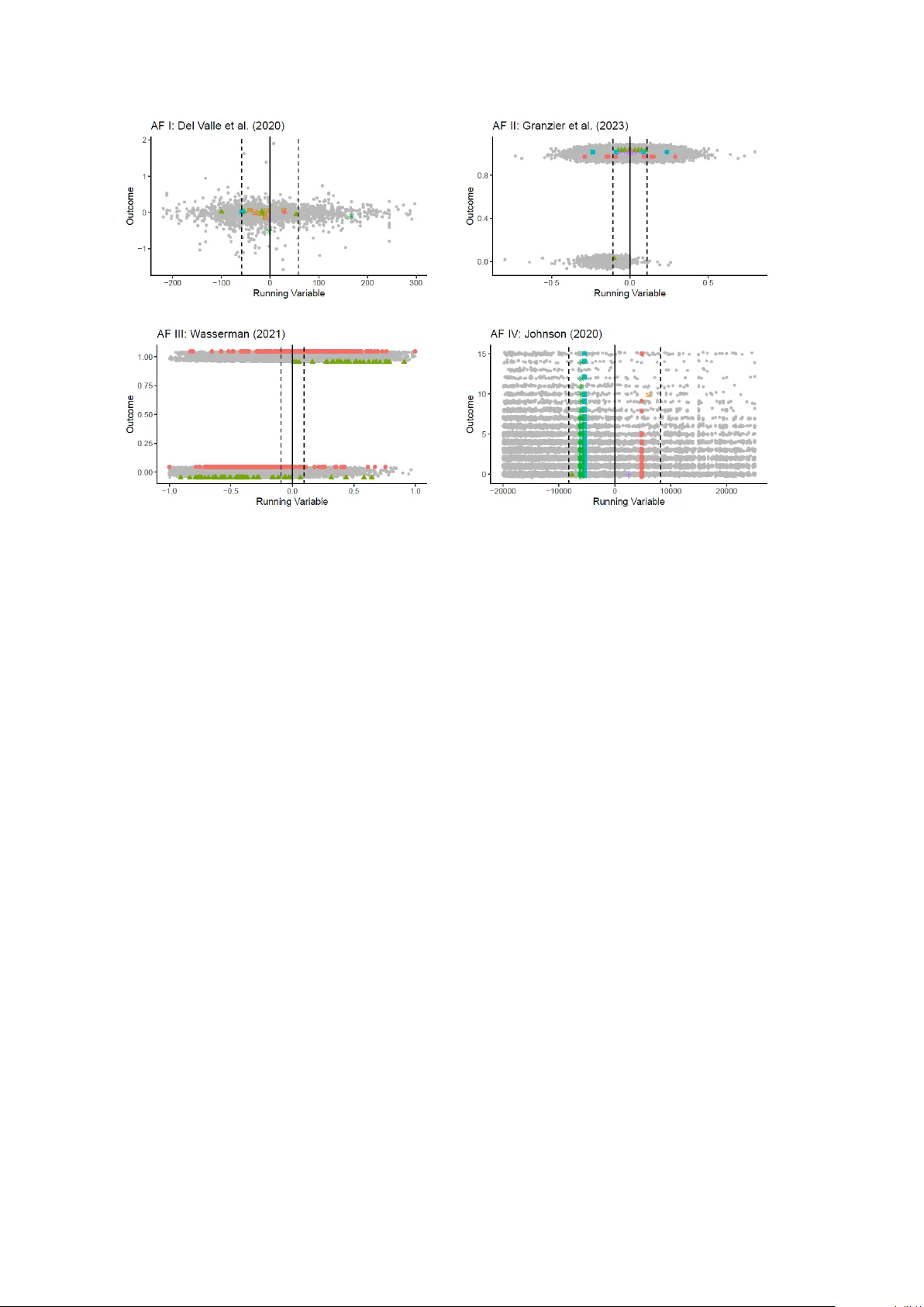
Inference in Regression Discon tin uit y Designs with Clustered Data Claudia Noac k T omasz Olma Christoph Rothe Abstract Clustered sampling is prev alen t in empirical regression discontin uit y (RD) de- signs, but it has not received m uch atten tion in the theoretical literature. In this pap er, w e in tro duce a general mo del-based framew ork for such settings and de- riv e high-level conditions under whic h the standard local linear RD estimator is asymptotically normal. W e v erify that our high-lev el assumptions hold across a wide range of empirical designs, including settings of growing cluster sizes. W e further sho w that clustered standard errors that are currently used in practice can b e either inconsistent or o v erly conserv ative in ﬁnite samples. T o address these issues, we prop ose a no vel nearest-neighbor-type v ariance estimator and illustrate its prop erties in a div erse set of empirical applications. This v ersion: March 20, 2026. W e thank Deb opam Bhattac harya, Morten Nielsen, Zhuan Pai and n umerous seminar and conference participants for helpful comments and suggestions. The second author gratefully ackno wledges ﬁnancial support from the Europ ean Researc h Council ERC through gran t SH-1852332. A uthor contact information: Claudia Noack, Departmen t of Economics, Univ ersity of Bonn. E-Mail: claudia.noack@uni-bonn.de. W ebsite: https://claudianoac k.github.io. T omasz Olma, Departmen t of Statistics, Ludwig Maximilian Univ ersity of Munich. E-Mail: t.olma@lmu.de. W ebsite: h ttps://tomaszolma.github.io. Christoph Rothe, Departmen t of Economics, Universit y of Mannheim. E-Mail: rothe@vwl.uni-mannheim.de. W ebsite: h ttp://www.c hristophrothe.net. 1 1. INTR ODUCTION Regression discontin uit y (RD) designs are widely applied in economics and other so cial sciences. In these settings, treatment is assigned whenever a unit’s realization of the running v ariable crosses a known cutoﬀ; for instance, a candidate is elected only if their v ote share exceeds 50%. Under con tinuit y conditions on the conditional exp ectations of the p oten tial outcomes, the a v erage treatment eﬀect at the cutoﬀ is iden tiﬁed b y the jump in the conditional exp ectation of the observed outcome giv en the running v ariable at the cutoﬀ. This jump is t ypically estimated as the diﬀerence of the lo cal linear estimates on either side of the cutoﬀ. Most theoretical results on estimation and inference in RD designs are deriv ed in set- tings where the researcher observes a sample of indep endent and iden tically distributed (i.i.d.) observ ations drawn from a large p opulation (e.g., Hahn et al., 2001; Imbens and Kaly anaraman, 2012; Calonico et al., 2014; Armstrong and Kolesár, 2020). In practice, ho wev er, applied researc hers often regard the i.i.d. assumption as unrealistic and rou- tinely rep ort clustered standard errors. F or example, we revisited the surv ey of recent RD studies published in the journals of the American Economic Asso ciation conducted b y Noac k et al. (2025) and found that clustered standard errors were used in around 80% of the surv eyed articles. Despite the prev alence of clustered sampling in applied RD studies, formal results for lo cal linear RD estimators – and more generally lo cal p olyno- mial regression – under such dep endence structures remain limited. In particular, the existing literature oﬀers little guidance on the conditions under whic h these estimators are asymptotically normal across the range of clustering patterns encoun tered in practice, or on how to conduct v alid inference in such settings. This pap er mak es tw o main con tributions. First, w e pro vide an asymptotic theory for the lo cal linear RD estimator for clustered data with a large num b er of indep en- den t groups. F rom a statistical p ersp ective, RD estimators are weigh ted av erages of the outcome v ariable where the weigh ts dep end on the running v ariable, the k ernel, and the bandwidth. When units are clustered, the interaction betw een lo cal weigh ting and within- cluster dep endence alters the asymptotic b eha vior of the lo cal linear RD estimator. W e deriv e high-lev el conditions under whic h the lo cal linear RD estimator is asymptotically normally distributed. These conditions are form ulated in terms of the weigh ts assigned to units from diﬀeren t clusters and translate in to restrictions on cluster sizes within the estimation window. T o relate our high-lev el conditions to empirically relev an t designs, we in tro duce four stylized asymptotic framew orks motiv ated by empirical RD applications. These frameworks capture ho w the asymptotic b eha vior of lo cal linear RD estimators de- p ends on (i) the eﬀective n umber of units p er cluster within the estimation windo w, (ii) the dep endence structure of the running v ariable within clusters, and (iii) assumptions on 2 the within-cluster cov ariance structure of the outcome. Within these framew orks, w e ﬁnd that distinct con vergence rates and optimal bandwidth c hoices are qualitativ ely diﬀeren t from i.i.d. settings. Our results complement the analysis of Hansen and Lee (2019) by considering nonparametric mo dels. In contrast to their analysis, where the estimators are based on the full sample, the lo calization of the RD estimator leads to non-standard con vergence rates. Second, we consider estimation of the conditional v ariance of the lo cal linear RD esti- mator. W e show that the con v entional clustered regression residual-based standard error is consistent under the same cluster size conditions that ensure asymptotic normality of the RD estimator. How ev er, in settings with independent data, the regression residual- based standard errors are kno wn to exhibit less ﬁnite-sample bias than the so-called nearest-neigh b ors standard errors. A naive adaptation of the nearest-neighbors standard error for indep endent data to clustered settings is in v alid, and to our kno wledge, no v alid nearest-neigh b ors-type standard error for clustered RD designs currently exists. As the second main contribution, we propose a no vel clustered nearest-neigh b ors (CNN) stan- dard error for RD estimators. Our prop osed metho d chooses nearest neighbors taking in to account the clustering structure and exploiting indep endence b etw een clusters. W e establish consistency of our prop osed CNN standard error under our high-level assump- tions on the cluster sizes. 1 W e complement our theoretical analysis with empirical applications that assess the ﬁnite-sample p erformance of the prop osed standard error relativ e to existing alternativ es. Related Literature. Cluster-robust inference is routinely emplo yed in empirical RD designs. Despite this fact, formal results remain limited, even for the standard nonpara- metric regression using lo cal p olynomial estimators. F or RD designs with clustering, Bartalotti and Brummet (2017) sho w asymptotic normality of lo cal p olynomial RD esti- mators under the assumption that all clusters are of the same size and the realizations of the running v ariable are on the same side of the cutoﬀ within eac h cluster. Clustered standard errors hav e been implemen ted in popular RD pac kages rdrobust and RDHonest without m uch theoretical foundation. Our pap er contributes to this literature b y pro vid- ing a uniﬁed theory for all common RD v arian ts with arbitrary clustering. Lin and Carroll (2000), W ang (2003), and Bhattac harya (2005) study general local p olynomial estimators under b ounded cluster sizes. In these regimes, as the bandwidth con verges to zero, the probability of ha ving more than one unit within the estimation windo w conv erges to zero for any given cluster, and in consequence, the clustering do es 1 Although our CNN standard error is dev elop ed for RD designs in this pap er, the general idea b ehind it extends naturally to other conditional inference problems under missp eciﬁcation, such as those studied b y Abadie et al. (2014). 3 not aﬀect the asymptotic distribution. Shimizu (2025) studies nonparametric density and lo cal p olynomial estimation under clustered sampling with heterogeneous and p o- ten tially unbounded cluster sizes. How ev er, his framework imposes restrictions that rule out several empirically relev an t RD settings. In particular, cluster sizes within the esti- mation windo w are required to remain uniformly bounded in exp ectation, the cov ariates are not allow ed to b e perfectly dep endent within a cluster, and the within-cluster co v ari- ance structure of the residuals takes on a v ery sp eciﬁc form. F urthermore, his prop osed v ariance estimator relies on parametric assumptions. By con trast, our framew ork accom- mo dates w eaker conditions on cluster sizes, allo ws for more general dep endence structures in the running v ariable within clusters, and imp oses milder assumptions on the cov ariance functions, while still delivering asymptotic normality . Moreov er, our prop osed nearest- neigh b or standard error is fully nonparametric and do es not rely on parametric mo deling assumptions. In settings of regular parameters, there is a v ast literature about cluster-robust infer- ence. Liang and Zeger (1986); White (2014); Arellano (1987) pro vide the foundational large- G theory for cluster-robust co v ariances for b ounded cluster sizes; see Cameron and Miller (2015); MacKinnon et al. (2023) for reviews. Djogb enou et al. (2019); Hansen and Lee (2019); Bugni et al. (2025); Hansen (2025) extend the results to unequal, p ossibly large clusters. Abadie et al. (2023) discuss clustering adjustmen ts from a design-based p ersp ectiv e. Chiang et al. (2025) p oin t out that in man y empirical applications the size of the largest cluster is not negligible relative to the total sample size, and they provide an alternativ e b o otstrap inference pro cedure. This pap er is the ﬁrst to propose and formally study a cluster-robust nearest-neigh b ors- t yp e standard error. In this regard, w e extend the work of Abadie et al. (2014), who sho wed consistency of the nearest-neigh b ors standard errors under i.i.d. sampling (in a more general class of missp eciﬁed mo dels). Plan of the Paper. Section 2 in tro duces the mo del and giv es a preview of our main results. Section 3 states the high-lev el assumptions and establishes asymptotic normality of the lo cal linear RD estimator. Section 4 studies the asymptotic frameworks. Section 5 in tro duces our prop osed standard error and w e sho w that it is consisten t. Section 6 con tains the empirical applications. All pro ofs are collected in the App endix. 2. SETTING AND PREVIEW OF THE RESUL TS 2.1. Clustered Sampling. W e consider a sharp RD design, in whic h a unit receives the treatmen t if and only if their running v ariable exceeds a kno wn cutoﬀ v alue, which we normalize to zero. The observed data is divided in to G clusters, and in each cluster, w e observ e n g units. Let X g i and Y g i denote the running v ariable and the outcome v ariable 4 of observ ation i in cluster g , resp ectiv ely . The total sample size is given by n = P g ∈ [ G ] n g , where [ G ] = (1 , . . . , G ) . In our asymptotic analysis, w e will treat G and ( n g ) g ∈ [ G ] as deterministic sequences indexed by the sample size n . Observ ations in diﬀeren t clusters are indep endent, but they can b e dependent within a cluster. The outcome is generated according to the mo del Y g i = µ ( X g i ) + ε g i , (2.1) where µ ( x ) = E [ Y g i | X g i = x ] , E [ ε g i |X g ] = 0 , X g = ( X g i ) i ∈ I g , and I g = (1 , . . . , n g ) . The error terms ε g i can b e arbitrarily dep enden t within a cluster. W e denote their v ariance and co v ariances, conditional on X g b y σ 2 g ,i = V ar( Y g i |X g ) , σ g ,ij = Co v( Y g i , Y g j |X g ) , and w e denote the co v ariance matrix of Y g = ( Y g i ) i ∈ I g conditional on X g b y Σ g . Under con tinuit y assumptions on the conditional exp ectation of the p oten tial out- comes, the jump in the conditional exp ectation µ ( x ) at the cutoﬀ iden tiﬁes the a verage treatmen t eﬀect of units at the cutoﬀ (Hahn et al., 2001). Our parameter of in terest is therefore giv en b y τ = µ (0 + ) − µ (0 − ) , where for a generic function f , f (0 + ) and f (0 − ) denote the righ t and left limits of the function f at zero. Remark 1. In the mo del of observ ed data in (2.1), we assume that the conditional exp ectation function µ is the same in each cluster in the sample. W e note that this mo del allows for sampling from a p opulation where clusters are heterogeneous in terms of µ if, in eac h rep eated sample keeping ( n g ) g ∈ [ G ] ﬁxed, the observ ed clusters are drawn at random from the sup erp opulation of clusters of inﬁnite size. Sp eciﬁcally , supp ose that w e dra w a random set of clusters G = { ˜ g 1 , . . . , ˜ g G } and observ e a sample of random units from these clusters, { ( X ˜ g i , Y ˜ g i ) i ∈ [ I ˜ g ] } ˜ g ∈G . If w e assume that Y ˜ g i = µ ˜ g ( X ˜ g i ) + η ˜ g i , E [ η ˜ g i |X ˜ g ] = 0 , then this mo del ﬁts in to our framework if w e deﬁne µ ( x ) = E [ µ ˜ g ( x )] and ε ˜ g i = η ˜ g i + µ ˜ g ( X ˜ g i ) − µ ( X ˜ g i ) , where the exp ectation is tak en w.r.t. the distribution of clusters in the p opulation. 5 2.2. Lo cal Linear RD Estimator. In practice, it is common to estimate the RD pa- rameter via lo cal linear RD regressions. This estimator is deﬁned as b τ ( h ) = e ⊤ 1 argmin β ∈ R 4 n X i =1 k h ( X i )( Y i − V ⊤ i β ) 2 ≡ X g ∈ [ G ] X i ∈ I g w g i ( h ) Y g i , (2.2) where V i = ( T i , X i , T i X i , 1) ⊤ , k h ( v ) = k ( v /h ) /h with k ( · ) a kernel function and h > 0 a bandwidth, and e 1 = (1 , 0 , 0 , 0) ⊤ is the ﬁrst unit v ector. The weigh ts w g i ( h ) dep end only on the running v ariable and the bandwidth; the exact expressions for the weigh ts are given in App endix C.1. In our setting, the v ariance of the RD estimator conditional on the running v ariable X n = ( X g ) g ∈ [ G ] equals se 2 ( h ) ≡ V ar( b τ ( h ) |X n ) = X g ∈ [ G ] X i,j ∈ I g w g i ( h ) w g j ( h ) σ g ,ij . (2.3) 2.3. Preview of Asymptotic Results. Our ﬁrst main result establishes the large-sample b eha vior of the RD estimator under clustered sampling. W e derive it under high-lev el conditions on the w eights w g i ( h ) that translate in to restrictions on cluster sizes within the estimation windo w. Under these general high-level conditions, we sho w that the lo cal linear RD estimator is asymptotically normal: se ( h ) − 1  b τ ( h ) − E [ b τ ( h ) | X n ]  d − → N (0 , 1) . The con vergence rate of the conditional v ariance se 2 ( h ) dep ends on the cov ariance of outcomes within eac h cluster, Σ g , the join t distribution of the realizations of the running v ariable within eac h cluster, X g , and the cluster sizes, and it can b e slow er than the con vergence rate of ( nh ) − 1 obtained in i.i.d. settings. F or example, w e sho w in Section 4 that if the joint distribution of X g admits a b ounded densit y and some mild regularit y conditions hold, then se 2 ( h ) = O P  1 + λ n nh  , where λ n = h n X g ∈ [ G ] n g ( n g − 1) . If, in turn, the distribution of X g is degenerate, meaning that the realizations of the running v ariable are equal within each cluster, then se 2 ( h ) = O P  1 + λ n /h nh  . The ab ov e results provide b ounds on the conv ergence rate of the conditional v ariance 6 se 2 ( h ) . Whether these rates are binding dep ends on the exact form of the conditional co v ariance matrix Σ g . In Section 4.4, we giv e an example where these b ounds are ac hieved, but w e note that the conv ergence rate of se 2 ( h ) can b e faster. F or example, in the case of b ounded joint densit y , if the residuals are uncorrelated within each cluster, then se 2 ( h ) = O P (( nh ) − 1 ) , as in the i.i.d. case, ev en if λ n div erges to inﬁnit y . 2.4. Standard Errors. Reliable and eﬃcient inference requires a v ariance estimator that is b oth consisten t and w ell-b ehav ed in ﬁnite samples. Natural estimates of se 2 ( h ) are of the form b se 2 ( h ) = X g ∈ [ G ] X i,j ∈ I g w g i ( h ) w g j ( h ) b σ g ,ij (2.4) with b σ g ,ij b eing some estimate of σ g ,ij . Setting b σ g ,ij to the pro duct of residuals from the lo cal linear RD regression asso ciated with observ ations i and j in cluster g yields a clustered regression residual-based standard error, analogous to the cluster-robust stan- dard errors prop osed for the linear regression (Liang and Zeger, 1986). W e show that this standard error is v alid under the same high-level conditions on the weigh ts as those ensuring asymptotic normality . Ev en though the regression residual-based standard error is consistent under mild assumptions, it has b een long recognized in i.i.d. settings that this approach may b e ov erly conserv ative in ﬁnite samples, and the nearest-neighbors standard error has b een prop osed to alleviate this issue (Abadie et al., 2014). A t its core, the nearest-neighbors approach estimates the conditional v ariance of the outcome v ariable for an y giv en observ ation using the outcome v ariabilit y among its nearest neigh b ors. A direct w ay to adapt the nearest-neighbors v ariance estimation approac h to clustered data is to set b σ g ,ij in equation (2.4) to b σ naive g ,ij = Y ∆ , naive g i Y ∆ , naive g j , Y ∆ , naive g i = s |N naive g i | 1 + |N naive g i |   Y g i − 1 |N naive g i | X ( g ′ ,i ′ ) ∈N naive gi Y g ′ i ′   , where N naive g i is the set of J units that are closest to unit i in cluster g in terms of the running v ariable. 2 Ho wev er, this pro cedure do es not take into account the clustering structure, and there is no reason to expect that such a v ariance estimator is consisten t in general. First, if the c hoice of neighbors is associated with cluster mem b ership, then an additional bias term can b e present. Second, the bias-correction factor is devised for v ariance estimation, but it turns out it is not suitable for cov ariance estimation. W e giv e t wo illustrativ e examples showing these problems in Section 5.1.1. 2 A standard error of that t yp e was proposed by Calonico et al. (2019, Supplemen tal App endix 7.10) and is implemen ted in the softw are package rdrobust . W e note that this approach also assumes that residuals are uncorrelated across observ ations on opposite sides of the cutoﬀ. 7 T o remedy the deﬁciencies of the naive approac h, w e prop ose a diﬀerent clustered nearest-neigh b ors standard error where b σ g ,ij is set to b σ CNN g ,ij = Y ∆ 1 g i Y ∆ 2 g j , Y ∆ d g i ≡ Y g i − 1 |N d g i | X ( g ′ ,i ′ ) ∈N d gi Y g ′ i ′ for d ∈ { 1 , 2 } , where N 1 g i and N 2 g i are carefully chosen sets of neighbors of observ ation i in cluster g . Crucially , w e require that the observ ations in ∪ i ∈ I g N 1 g i and ∪ i ∈ I g N 2 g i b elong to tw o disjoin t sets of clusters not including g . Under this requirement and additional assumptions w e sho w this standard error is consisten t, and one can see in sim ulations that our procedure has fav orable ﬁnite-sample prop erties, exhibiting a smaller bias relative to the regression residual-based approac h is settings where the curv ature of µ is substantial. 3. ASYMPTOTIC NORMALITY UNDER HIGH-LEVEL CONDITIONS In this section, w e sho w asymptotic normalit y of the lo cal linear RD estimator under high-lev el assumptions on the w eights. 3.1. High-Lev el Conditions. The ﬁrst assumption controls the cluster sizes in terms of the weigh ts assigned to units in eac h cluster. Assumption 1. (i) max g ∈ [ G ] X i,j ∈ I g | w g i ( h ) w g j ( h ) | /se 2 ( h ) = o P (1) , (ii) X g ∈ [ G ] X i,j ∈ I g | w g i ( h ) w g j ( h ) | /se 2 ( h ) = O P (1) . Assumption 1 puts restrictions on the size of the terms P i,j ∈ I g | w g i ( h ) w g j ( h ) | . In our asymptotic analysis, it is used to control the con tributions of diﬀeren t clusters to the conditional v ariance se 2 ( h ) . This assumption allows the n umber of non-zero w eights within each cluster to gro w with the sample size, as long as none of the clusters dominates all others in terms of the sums of the absolute v alue of cross-pro ducts of the w eights. This assumption is v ery general and w e pro vide a range of diﬀerent asymptotic framew orks in whic h it is satisﬁed in Section 4. Ho wev er, w e note that it is a suﬃcient condition to obtain asymptotic normality , but it is not necessary . In particular, it do es not co ver settings where the n um b er of clusters does not increase with the sample size. F or example, if there is one cluster of weakly-dependent data (e.g., strongly mixing pro cess, as extensiv ely studied in time-series settings), one migh t still obtain asymptotic normalit y , but part (i) of the assumption will generally not hold. 8 Remark 2. Assumption 1 do es not require the weigh ts w g i ( h ) to b e deriv ed via a lo cal linear regression. It is compatible with any estimator that is a w eighted mean of out- comes where the weigh ts do not dep end on the outcome v ariable, e.g., higher-order local p olynomial estimators or the optimized RD estimators (Im b ens and W ager, 2019; Ghosh et al., 2025). The second assumption con trols the moments of the error terms and is standard for results in voking cen tral limit theorems with non-i.i.d. data. Assumption 2. E [ | ε g i | δ |X g ] is uniformly b ounde d for some δ > 2 for al l g ∈ [ G ] and i ∈ I g . 3.2. Asymptotic Normality. Our ﬁrst main result establishes asymptotic normalit y of the RD estimator. T o control its bias, w e introduce the Hölder-type class of real functions that are p otentially discon tin uous at zero, are t wice diﬀerentiable on either side of the threshold, and whose second deriv ativ es are uniformly b ounded by some constant M > 0 : F H ( M ) = { f 1 ( x ) 1 { x ≥ 0 } − f 0 ( x ) 1 { x < 0 } : ∥ f ′′ w ∥∞ ≤ M , w = 0 , 1 } . Theorem 1. (i) Supp ose that A ssumptions 1 and 2 hold. Then, c onditional on X n , b τ ( h ) − E [ b τ ( h ) |X n ] se ( h ) d − → N (0 , 1) . (ii) F or any M ≥ 0 , sup µ ∈F H ( M )   E [ b τ ( h ) |X n ] − τ   ≤ ¯ b ( h ) ≡ − M 2 X g ∈ [ G ] X i ∈ I g w g i ( h ) X 2 g i sig n ( X g i ) . P art (i) of the theorem shows that b τ ( h ) , appropriately recentered and rescaled, is asymptotically normally distributed. Part (ii) shows that the conditional bias is bounded b y a quan tit y that is the pro duct of the b ound on the second deriv ative of the conditional exp ectation function and an expression that dep ends only on the w eights and the running v ariable. The bias bound is the same as in the i.i.d. setting (Armstrong and Kolesár, 2020; Noac k and Rothe, 2024) since the lo cal linear RD estimator is a linear op erator and its conditional exp ectation is not aﬀected b y the dep endence across outcomes. Giv en the standard deviation of the lo cal linear RD estimator and a b ound on its bias, w e will consider the conditional worst-case mean squared error o v er data-generating pro cess with µ ∈ F H ( M ) : M S E ( h ) = ¯ b ( h ) 2 + se 2 ( h ) . W e will explicitly derive the limit of M S E ( h ) and characterize the corresp onding asymp- totically optimal bandwidth under low-lev el conditions in the next section. 9 4. ASYMPTOTIC FRAMEWORKS Our high-lev el Assumption 1 in tro duced in Section 3 accommo dates a wide range of empirical clustering structures. T o illustrate this ﬂexibility , we formalize four asymptotic framew orks and pro vide low-lev el conditions under whic h the high-lev el assumption holds. Eac h of the asymptotic framew orks is calibrated to a class of empirical RD applications. They diﬀer in (i) ho w quickly the num b er of near-cutoﬀ units can gro w inside a cluster, (ii) the dep endence structure of the running v ariable within clusters, and (iii) assumptions on the conditional cov ariance matrix of the outcome. A symptotic F r ameworks I and II are motiv ated b y empirical applications where there are man y clusters that can b e p otentially large, but the num ber of units from an y cluster within the estimation windows is relatively small. They co ver tw o distinct dependence patterns in the running v ariable. While Asymptotic F ramew ork I assumes that the join t distribution of the running v ariable within eac h cluster admits a bounded join t density , Asymptotic F ramework II do es not put an y restrictions on this distribution at the cost of imp osing stronger restrictions on the rates of the cluster sizes. A symptotic F r ameworks III and IV relax the restrictions on cluster sizes imp osed in Asymptotic F ramew orks I and I I, resp ectively , while instead requiring additional assumptions on the cov ariance structure of the outcome residuals. W e discuss represen tative empirical examples of eac h of the asymptotic frameworks in Section 6.2. 4.1. General Assumptions. W e will ﬁrst presen t general assumptions that are main- tained in all the four asymptotic framew orks. Assumption 3. (i) The mar ginal distribution of X g i is the same for al l g ∈ [ G ] and i ∈ I g , and it admits a c ontinuous density f X that is b ounde d away fr om zer o ar ound the cutoﬀ. (ii) The kernel function k is a b ounde d and symmetric density function with b ounde d supp ort, say [ − 1 , 1] . (iii) h → 0 and nh → ∞ . P art (i) of Assumption 3 matc hes standard conditions for lo cal polynomial estimation with con tinuously distributed regressors (F an and Gijb els, 1996). W e imp ose contin uit y (and contin uit y at the cutoﬀ ) only to obtain simple closed-form v ariance limits; our high-lev el results can also accommo date discrete, mixed, or cutoﬀ-discontin uous running v ariables under suitable mo diﬁcations to the v ariance calculations. In the same spirit, we assume the density is contin uous at the cutoﬀ to simplify the formulas; formally , an RD analysis can pro ceed without this requiremen t, and our main results remain unaﬀected if the running v ariable is discon tinuous at the threshold. The kernel and bandwidth requiremen ts in parts (ii) and (iii) are standard in the nonparametric regression literature. W e note that the assumption that the bandwidth 10 shrinks to zero is not necessary for our high-lev el conditions to hold. W e could accom- mo date a ﬁxed bandwidth; we main tain the usual condition that the bandwidth shrinks to zero solely to obtain closed-form expressions for the leading bias and v ariance terms. In the asymptotic results, we will use the following k ernel constan ts. F or j ∈ N , let ¯ µ j = R 1 0 k ( v ) v j dv . F urther, deﬁne ¯ µ = ( ¯ µ 2 2 − ¯ µ 1 ¯ µ 3 ) / ( ¯ µ 2 ¯ µ 0 − ¯ µ 2 1 ) and ¯ κ = R 1 0 ¯ k ( v ) 2 dv , where ¯ k ( v ) = k ( v )( ¯ µ 2 − ¯ µ 1 v ) / ( ¯ µ 2 ¯ µ 0 − ¯ µ 2 1 ) . Assumption 4. (i) E [ | ε g i | 2 |X g ] is uniformly b ounde d for al l g ∈ [ G ] and i ∈ I g . (ii) The minimal eigenvalue of the c onditional c ovarianc e matrix of cluster g , λ min (Σ g ) , is b ounde d away fr om zer o uniformly in n and g ∈ [ G ] . P art (i) is slightly w eak er than Assumption 2. P art (ii) is imp osed to rule out degen- erate conditional dep endence structures in the outcome v ariable, suc h as situations where t wo residuals within the same cluster are p erfectly negatively correlated. The v ariance of the RD estimator could collapse to zero in such cases, precluding asymptotic normality . 4.2. Small Eﬀectiv e Cluster Sizes. The ﬁrst tw o asymptotic frameworks apply to settings where the num b er of units from an y cluster within the estimation window is relativ ely small. 4.2.1. A ssumptions. The num b er of units within the estimation windo w from any given cluster dep ends on the total n um b er of units in the cluster as w ell as the join t distribution of the running v ariable within the cluster. In Asymptotic F ramework I, w e assume that the join t distribution of the realizations of the running v ariable admits a b ounded joint densit y , while Asymptotic F ramework I I leav es the join t distribution unrestricted. Assumption AF-I. (i) The joint densit y of ( X g i 1 , . . . , X g i k ) is b ounded uniformly in n ∈ N , g ∈ [ G ] , and 1 ≤ i 1 < . . . < i k ≤ n g for k ∈ { 2 , . . . , n g } . (ii) λ n = O (1) . (iii) max g ∈ [ G ] n 2 g h 2 + log 2 G nh = o (1) . Assumption AF-I(i) excludes cases of p erfect within-cluster correlation in the running v ariable where all units share the same realization of the running v ariable; such extreme dep endence is allow ed under Assumption AF-II below at the cost of more restrictiv e rate conditions. Assumption AF-I is similar to Assumption 2 of Hansen and Lee (2019), who study the conv ergence of the av erage of clustered observ ations and other regular, full- sample estimators. Since we consider estimation using the data close to the cutoﬀ, our conditions are form ulated in terms of the “lo cal sample size” nh and the “lo cal cluster sizes” n g h , rather than the full sample size n and the cluster sizes n g used b y Hansen and Lee (2019). Another conceptual diﬀerence is that part (iii) includes an additional log G term. This extra factor is due to the randomness of cluster sizes within the estimation 11 windo w in our framework, whereas Hansen and Lee (2019) consider the setting of regular parameters and use all observ ations within eac h cluster. W e note that this asymptotic framew ork shares some similarities with the framew ork of Shimizu (2025) sp ecialized to one contin uous co v ariate. He also assumes that the joint distribution of the realizations of the running v ariable admits a joint densit y (albeit only for subsets of four observ ations) and λ n = O (1) . How ever, he imp oses a restrictive assumption that max g ∈ [ G ] n g h = O (1) , whereas our framework allo ws this quantit y to diverge. Assumption AF-II. (i) λ n = O ( h ) . (ii) max g ∈ [ G ] n 2 g nh = o (1) . Assumption AF-II imposes no restrictions on the joint density of the running v ariable, but the rate conditions on the cluster sizes are more stringent than in Assumption AF-I. In particular, it allo ws for the realizations of the running v ariable to be equal within eac h cluster. It turns out that this extreme case determines the restrictions on the cluster sizes that are necessary to verify Assumption 1. T o illustrate the restrictions imp osed in Assumptions AF-I and AF-I I, we consider tw o examples that diﬀer in the degree of allow ed heterogeneit y in cluster sizes. W e revisit these examples in the next subsection to facilitate comparisons b etw een asymptotic frameworks. Example 1. Supp ose that all clusters are of the same size, i.e., n g = n/G for all g ∈ [ G ] , then λ n = O ( n 1 h ) . The rate conditions in Assumption AF-I reduce to n 1 h = O (1) and log 2 G/ ( nh ) = o (1) and in Assumption AF-I I to n 1 = O (1) and Gh → ∞ . W e note that in Example 1, the exp ected num b er of units within the estimation win- do w remains b ounded in an y given cluster. The next example sho ws that b oth Asymp- totic F rameworks I and I I allo w the maximal expected num b er of observ ations within the estimation windo w to div erge for some clusters. Example 2. Let a ≥ b for a, b ∈ (0 , 1) . Supp ose that w e observe G 1 = n − ⌊ n a ⌋ clusters of size 1 and G 2 = ⌊ n b ⌋ clusters of size ⌊ n a − b ⌋ . F urther, for illustration, assume that h = n − b . Then λ n = O ( n − b + n 2( a − b ) − 1 ) . The rate conditions of Assumption AF-I hold if a ≤ b + 1 2 . In addition, if a > 2 b , then each large cluster contributes a div erging num b er of units lo cal to the cutoﬀ, since max g ∈ [ G ] n g h ≍ n a − 2 b → ∞ . The rate conditions of Assumption AF-I I holds provided a < 1 2 (1 + b ) . 4.2.2. The or etic al r esults. The follo wing prop osition presen ts our k ey theoretical results for Asymptotic F ramew orks I and I I. Prop osition 1. Supp ose that A ssumptions 3, 4, and either A ssumption AF-I or AF-II holds. Then A ssumption 1 is satisﬁe d, se 2 ( h ) ≍ p ( nh ) − 1 , and ¯ b ( h ) = − M ¯ µh 2 (1 + o P (1)) . 12 Prop osition 1 veriﬁes our high-lev el condition on the weigh ts, sho ws that the condi- tional v ariance of the RD estimator is of order ( nh ) − 1 , and it c haracterizes the leading term of the conditional w orst-case bias ¯ b ( h ) . It follo ws that w orst-case asymptotic mean squared error is of order h 4 + ( nh ) − 1 , which is minimized for bandwidths of order n − 1 / 5 . With such a bandwidth, the estimator conv erges at the rate n − 2 / 5 , giv en that our assump- tions hold for this bandwidth c hoice. W e note that the order of the v ariance is the same as in the i.i.d. case, but its exact form is in general aﬀected b y clustering; we deriv e its limit under additional assumptions in Section 4.4. 4.3. Large Eﬀectiv e Cluster Sizes. While Asymptotic F rameworks I and I I cov er man y relev ant clustering patterns, the conditions on the growth rates of the cluster sizes migh t b e restrictiv e in some applications. In this section, w e show these rate conditions can be signiﬁcan tly relaxed under direct assumptions on the standard error. W e then argue in Section 4.4 that these assumptions are reasonable in many settings. 4.3.1. A ssumptions. Asymptotic F ramew ork I I I considers cases where the joint distribu- tion of the realizations of the running v ariable is con tinuous, as in Asymptotic F rame- w ork I, but it relaxes the rate conditions imp osed on the cluster sizes. This asymptotic framew ork is motiv ated by settings where the clusters hav e a large num b er of units even in a shrinking neighborho o d of the cutoﬀ. Assumption AF-II I. (i) The joint densit y of ( X g i 1 , . . . , X g i k ) is bounded uniformly in n ∈ N , g ∈ [ G ] , and 1 ≤ i 1 < . . . < i k ≤ n g for k ∈ { 2 , . . . , n g } . (ii) λ n nh + max g ∈ [ G ] ( n g h ) 2 + log 2 G nh (1 + λ n ) = o (1) . (iii) se 2 ( h ) ≍ p (1 + λ n ) / ( nh ) . P art (i) of Assumption AF-I I I coincides with part (i) of Assumption AF-I. Ho wev er, the rate conditions on cluster sizes in part (ii) are considerably w eaker than those imp osed in parts (ii) and (iii) of Assumption AF-I. In particular, λ n is allow ed to div erge to inﬁnity within this framework. Asymptotic F ramew ork IV applies to settings where eac h cluster may contain man y units whose realizations of the running v ariable might b e highly correlated. As a result, ev en within a shrinking neighborho o d of the cutoﬀ, some clusters can contribute a large n umber of units concentrated in a narrow region of the supp ort of the running v ariable. Suc h settings occur naturally , for example, if the outcomes are measured at the individual lev el, whereas the running v ariable is assigned at the cluster lev el. Assumption AF-IV. (i) λ n nh + max g ∈ [ G ] n 2 g P g ∈ [ G ] n 2 g = o ( h ) . (ii) se 2 ( h ) ≍ p (1 + λ n /h ) / ( nh ) . 13 The rate conditions on cluster sizes are signiﬁcan tly w eaker than those in Assump- tion AF-I I as w e com bine these conditions with an additional assumption on the standard error. W e note that the rate conditions in Assumption AF-IV are stronger than those in Assumption AF-I I I; this is needed b ecause w e do not imp ose any assumptions on the join t distribution of the running v ariables. W e next illustrate the implications of these rate conditions in our examples studied ab o ve. Example 1 (Equal Cluster Sizes, con t’d) . Assumption AF-I I I requires that G → ∞ and n 2 h 2 /G → ∞ . In this setting, se 2 ( h ) = O (1 / ( nh ) + 1 /G ) . P art (i) of Assumption AF- IV reduces to the requiremen t that Gh → ∞ . W e emphasize that there is no separate restriction on the cluster size. Part (ii) implies that se 2 ( h ) = O (1 / ( Gh )) . Example 2 (Heterogeneous Cluster Sizes, con t’d) . The rate conditions of Assump- tion AF-I I I do not imp ose any additional restrictions. Moreo ver, if a > 2 b , at least one large cluster is lo cally inﬂuential, in the sense that max g ∈ [ G ] n g h ≍ n a − 2 b → ∞ . The rate conditions of Assumption AF-IV imp ose the same restrictions as in Asymptotic F ramework II. It has to hold that a < 1 2 (1 + b ) . 4.3.2. The or etic al r esults. The follo wing prop osition presen ts our k ey theoretical results for Asymptotic F ramew orks II I and IV. Prop osition 2. Supp ose that A ssumptions 3 and 4 hold, and either A ssumption AF-III or AF-IV holds. Then A ssumption 1 is satisﬁe d and ¯ b ( h ) = − M ¯ µh 2 (1 + o P (1)) . Prop osition 2 v eriﬁes our high-level Assumption 1 and characterizes the leading term of the conditional w orst-case bias ¯ b ( h ) . W e note that the rate of the optimal bandwidth and the resulting con vergence rate of the estimator are diﬀeren t than in the i.i.d. case or the case of small eﬀectiv e cluster sizes discussed in the previous section. Sp eciﬁcally , in F ramework II I, we hav e that b τ ( h ) − τ = O P   h 2 + 1 √ nh + s P g ∈ [ G ] n 2 g n 2   . In contrast to Asymptotic F ramework I, the third term in the remainder on the righ t- hands side can dominate the other terms. Since the bandwidth h app ears only in the ﬁrst t wo terms, the conv ergence rate is optimized if h ∼ n − 1 / 5 , in which case we obtain b τ ( h ) − τ = O P ( n − 2 / 5 +  P g ∈ [ G ] n 2 g /n 2  1 / 2 ) . W e note that if n − 2 / 5 = o  P g ∈ [ G ] n 2 g /n 2  1 / 2  and h ∼ n − 1 / 5 , then the v ariance dominates the bias under the optimal bandwidth c hoice, suc h that b τ ( h ) − τ se ( h ) d − → N (0 , 1) , 14 assuming that Assumption AF-I I I holds for this bandwidth choice. In F ramew ork IV, in turn, w e hav e that b τ ( h ) − τ = O P   h 2 + 1 √ nh   1 + s P g ∈ [ G ] n 2 g n     . The fastest possible con vergence rate is achiev ed for h ∼  1 + P g ∈ [ G ] n 2 g /n  /n  1 / 5 , yield- ing b τ ( h ) − τ = O P  n − 2 / 5 +  P g ∈ [ G ] n 2 g /n 2  2 / 5  , given that this bandwidth choice satisﬁes Assumption AF-IV. 4.4. Standard Error and Bandwidth Choice in a Sp ecial Case. T o illustrate the b eha vior of the lo cal linear RD estimator with clustered data, we will further consider a simpliﬁed setup, where exact characterization of the limit of the v ariance is p ossible. The follo wing assumption formalizes the setup. Assumption 5. F or al l g ∈ [ G ] and i ∈ I g , σ 2 i,g = σ 2 ( X g i ) and σ ij,g = σ ( X g i , X g j ) for some functions σ 2 ( · ) and σ ( · , · ) that ar e L -Lipschitz c ontinuous away fr om the cutoﬀ. Assumption 5 imp oses a common co v ariance b et ween an y tw o units and across clusters, and it imp oses contin uit y of the conditional v ariance and co v ariance functions. 3 4.4.1. Continuous Joint Distribution of the Running V ariable. W e ﬁrst study the standard error under Asymptotic F rameworks I and I I I. Lemma 1. Supp ose that A ssumptions 3, 4(i), and AF-III(i)-(ii) hold. Then (i) se 2 ( h ) = O P  1 + λ n nh  . (ii) If in addition A ssumption 5 holds and ( X g i , X g j ) , i  = j , i, j ∈ I g , ar e identic al ly distribute d with c ontinuous joint density f ( x 1 , x 2 ) , then se 2 ( h ) = 1 nh   ¯ κ X ⋆ ∈{ + , −} σ 2 (0 ⋆ ) f X (0) + λ n X ⋆, ⋄∈{ + , −} 1 ± { ⋆ = ⋄} σ (0 ⋆ , 0 ⋄ ) f (0 , 0) f X (0) 2 + o P (1 + λ n )   , wher e 1 ± { ⋆ = ⋄} = 1 if ⋆ = ⋄ and 1 ± { ⋆ = ⋄} = − 1 otherwise. Lemma 1 imposes only the w eak rate conditions on the cluster sizes of Asymptotic F ramework I I I, whic h, in particular, co ver Asymptotic F ramework I. First, the lemma pro vides an upp er b ound on the con v ergence rate of the conditional v ariance se 2 ( h ) , and then it derives its exact limit in a sp ecial case. Part (ii) demonstrates that the conditional 3 This type of assumption can b e rationalized b y mo dels studied in the functional data literature (see, e.g., Zhang and Chen, 2007). Shimizu (2025) also imp oses such an assumption. 15 v ariance is asymptotically equal to the sum of t wo terms. The ﬁrst one is driv en b y the v ariances of individual units and is the same as in the i.i.d. case. The second comp onent is due to the cov ariance betw een outcomes within a cluster; w e note this part depends neither on the bandwidth nor the choice of the kernel function. If λ n con verges to a p ositiv e constant, then the t wo terms are of the same order. If λ n con verges to zero, then the eﬀect of clustering on v ariance b ecomes asymptotically negligible; a similar result w as obtained b y Shimizu (2025) under stronger rate restrictions on the cluster sizes. If λ n div erges to inﬁnit y and P ⋆, ⋄∈{ + , −} 1 ± { ⋆ = ⋄} σ (0 ⋆ , 0 ⋄ )  = 0 , the co v ariance part dominates. Under the assumptions of part (ii) of Lemma 1, the worst-case mean squared error of b τ ( h ) satisﬁes M S E ( h ) =   M 2 ¯ µ 2 h 4 + V 1 nh + P g ∈ [ G ] n 2 g n 2 X ⋆, ⋄∈{ + , −} 1 ± { ⋆ = ⋄} σ (0 ⋆ , 0 ⋄ ) f (0 , 0) f X (0) 2   (1 + o P (1)) , where V 1 = ¯ κ f X (0) P ⋆ ∈{ + , −} σ 2 (0 ⋆ ) . The bandwidth minimizing the leading term is giv en b y h ∗ 1 =  V 1 4 M 2 ¯ µ 2  1 / 5 n − 1 / 5 , giv en that this bandwidth c hoice satisﬁed the assumptions of part (ii) of Lemma 2. The optimal bandwidth h ∗ 1 is the same as the AMSE-optimal bandwidth in the i.i.d. case. W e emphasize that this result relies on Assumption 5; under more general cov ariance structures, it need not hold. 4.4.2. De gener ate Joint Distribution of the R unning V ariable. W e no w study the standard error under Asymptotic F rameworks I I and IV. T o deriv e a closed-form expression for the limit of the conditional v ariance in this setting, we need to imp ose an additional assumption on the joint distribution of the running v ariable. F or illustration, w e consider the setting where all the realizations of the running v ariable are the same within cluster. Lemma 2. Supp ose that A ssumptions 3, 4, and AF-IV(i) hold. Then (i) se 2 ( h ) = O P  1 + λ n /h nh  (ii) If in addition A ssumption 5 holds and the r e alizations of the running variable ar e e qual within e ach cluster. Then se 2 ( h ) = 1 nh ¯ κ f X (0) X ⋆ ∈{ + , −}  σ 2 (0 ⋆ ) + λ n h σ (0 ⋆ , 0 ⋆ ) + o P  1 + λ n h   . Lemma 2 imposes only the w eak rate conditions on the cluster sizes of Asymptotic F ramework IV, whic h, in particular, co ver Asymptotic F ramework I I. First, the lemma 16 pro vides an upp er b ound on the con v ergence rate of the conditional v ariance se 2 ( h ) , and then it derives its exact limit in a sp ecial case. Under the assumptions of Lemma 2, the worst-case mean squared error of b τ ( h ) satisﬁes M S E ( h ) =  M 2 ¯ µ 2 h 4 + V 2 nh  (1 + o P (1)) , where V 2 = ¯ κ f X (0) P ⋆ ∈{ + , −}  σ 2 (0 ⋆ ) + σ (0 ⋆ , 0 ⋆ ) P g ∈ [ G ] n g ( n g − 1) /n  . In this setting, the bandwidth minimizing the leading term of the AMSE-optimal bandwidth is giv en by h ∗ 2 =  V 2 4 M 2 ¯ µ 2  1 / 5 n − 1 / 5 , assuming the assumptions of Lemma 2 hold for this bandwidth c hoice. 5. CLUSTERED ST AND ARD ERROR In this section, w e study v ariance estimation based on the nearest-neigh b ors and regres- sion residual-based approaches. 5.1. Clustered Nearest-Neigh b ors Standard Error. W e ﬁrst show wh y the naiv e adaptation of the nearest-neigh b ors approach devised for i.i.d. settings is in general not v alid with clustered data. W e then in tro duce our proposed clustered nearest-neigh b ors (CNN) standard error and show its consistency . 5.1.1. F ailur e of the Naive Cluster e d Ne ar est-Neighb ors Standar d Err or. T o highlight the main problems with the naiv e clustered nearest-neigh b ors standard error describ ed in Section 2.4, w e consider a simple setup with µ ( X ) = 0 , V ar( Y g i |X g ) = σ 2 , and J = 1 nearest neigh b or. W e discuss t w o examples that diﬀer in the assumptions on the join t distribution of the realizations of the running v ariable. First, supp ose that each cluster consists of only t wo observ ations and X g 1 = X g 2 for all g ∈ [ G ] , suc h that N naive g 1 = { ( g , 2) } and N naive g 2 = { ( g , 1) } . Then b se 2 naive ( h ) = 1 2 X g ∈ [ G ] w 2 g 1 ( h ) X i,j ∈ I g Y ∆ , naive g i Y ∆ , naive g j = 1 2 X g ∈ [ G ] w 2 g 1 ( h ) 4 X l =1 ( − 1) l ( ε g 1 − ε g 2 ) 2 | {z } =0 = 0 . Clearly , this standard error cannot b e consistent. While this is a very speciﬁc example, the same t yp e of problem arises more generally whenever the realizations of the running v ariable are highly concentrated within clusters. 17 Second, supp ose that the join t distribution of the running v ariable within each cluster admits a b ounded join t densit y . Consider t wo observ ations i, j ∈ I g , i  = j , and let ( g 1 , i ′ ) and ( g 2 , j ′ ) b e their resp ective nearest neigh b ors. Assume further that the clusters g , g 1 , and g 2 are pairwise diﬀerent, which o ccurs with high probability in this setup if all clusters are relativ ely small. Then, while it is easy to see that the conditional v ariance estimate is correctly cen tered, E  Y ∆ , naive g i  2 |X n  = σ 2 , the conditional cov ariance estimates are biased: E h Y ∆ , naive g i Y ∆ , naive g j |X n i = 1 2 E [ ε g i ε g j − ε g i ε g 2 j ′ − ε g j ε g 1 i ′ + ε g 1 i ′ ε g 2 j ′ |X n ] = 1 2 E [ ε g i ε g j |X n ] . It follo ws that b se 2 naive ( h ) is not correctly cen tered in general. 4 5.1.2. Our Pr op ose d Cluster e d Ne ar est-Neighb ors Standar d Err or. It is evident from the preceding discussion that selecting neighbors from distinct clusters induces certain inde- p endence restrictions that are instrumental for establishing conditional un biasedness of the standard error. W e leverage this insigh t to construct our prop osed standard error, explicitly enforcing the desired indep endence structure. F or ev ery cluster g ∈ [ G ] , we deﬁne tw o sets of its “companion clusters”, R 1 g ⊂ [ G ] and R 2 g ⊂ [ G ] . Next, for every i ∈ I g and d ∈ { 1 , 2 } , w e deﬁne N d g i as the set of at least J nearest neighbors of unit i in cluster g in terms of the running v ariable that are on the same side of the cutoﬀ as X g i and b elong to a cluster in the set R d g . Our prop osed clustered nearest-neigh b ors (CNN) standard error is then deﬁned as: b se 2 C N N ( h ) = X g ∈ [ G ] X i,j ∈ I g w g i ( h ) w g j ( h ) Y ∆ 1 g i Y ∆ 2 g j , Y ∆ d g i ≡ Y g i − 1 |N d g i | X ( g ′ ,i ′ ) ∈N d gi Y g ′ i ′ . (5.1) T o show consistency of this standard error, w e require the sets of nearest neigh b ors to satisfy tw o properties. First we require that the neigh b ors in the t wo sets N 1 g i and N 2 g i are indep endent of the units in cluster g and of eac h other. This is achiev ed b y selecting companion clusters that do not include cluster g , g / ∈ R 1 g ∪ R 2 g , and are disjoin t, R 1 g ∩ R 2 g = ∅ . These prop erties ensure that our standard error is asymptotically conditionally un biased. Second, we need to con trol the dep endence b etw een P i,j ∈ I g w g i ( h ) w g j ( h ) Y ∆ 1 g i Y ∆ 2 g j across diﬀeren t clusters. W e achiev e that b y imp osing that eac h cluster can b e a com- panion cluster for at most R clusters for some ﬁxed num ber R , i.e., for all g ∈ [ G ] , w e 4 W e note that the problem arising in the naiv e conditional co v ariance estimation can b e easily resolv ed b y leaving out the correction factor when i  = j . How ever, a complete proof of approximate un biasedness of the standard error would still require controlling the probability of the resp ective clusters b eing distinct across all observ ations, limiting the applicabilit y of this metho d to relativ ely small clusters with a bounded joint density of the realizations of the running v ariable. 18 require #  ˜ g ∈ [ G ] : g ∈ R 1 ˜ g ∪ R 2 ˜ g  ≤ R. (5.2) These general requirements on the c hoice of companion clusters can b e satisﬁed by man y diﬀeren t selection metho ds. W e provide one concrete algorithm in App endix A. Remark 3. W e note that b se 2 C N N ( h ) does not reduce to the nearest-neighbors standard error that is typically used in i.i.d. settings. The standard nearest-neighbors standard errors replaces the unknown conditional v ariances with the squares of distances to nearest neigh b ors and it in volv es a bias-correction factor. Since we eﬀectiv ely tak e the pro duct of t wo diﬀeren t residuals, it turns out that this bias-correction factor is not needed. 5.1.3. Consistency of the CNN Standar d Err or. As is standard for nearest-neigh b ors-type estimators, our method relies on the assumption that the nearest neigh b ors selected in the construction of b se 2 C N N ( h ) are uniformly close to the resp ective units. Assumption 6. D ( h ) ≡ max g ∈ [ G ] max i ∈ I g w gi ( h )  =0 max ( ˜ g ,j ) ∈N 1 gi ∪N 2 gi | X g i − X ˜ g j | = o P (1) . This assumption is automatically satisﬁed whenever the nearest neighbors are selected within the estimation windo w, as is the case for the algorithm given in App endix A, and the bandwidth conv erges to zero. Since all matc hed units then lie within distance h of eac h other, w e ha ve D ( h ) = O ( h ) by construction. In general, we exp ect D ( h ) to conv erge to zero at a m uch faster rate. F or illustration, consider a setting where the marginal densit y of X g i is b ounded and b ounded a wa y from zero in a neighborho o d of the cutoﬀ. If the realizations of the running v ariable are constan t within each cluster and Gh → ∞ , then w e exp ect that D ( h ) = O P (log( Gh ) /G ) . As a diﬀerent example, consider a setting where the join t densit y of X g is con tinuous for all g ∈ [ G ] and n min h ≡ min g ∈ [ G ] n g h → ∞ , then w e exp ect that D ( h ) = O P (log( n min h ) /n min ) . Our second main result states that b se 2 C N N ( h ) is consistent for se 2 ( h ) . Theorem 2. Supp ose that A ssumptions 1 and 6 hold and A ssumption 2 holds with δ = 4 . Then b se 2 C N N ( h ) se 2 ( h ) = 1 + o P, F (1) , wher e the term o P, F (1) c onver ges to zer o uniformly over any class of DGPs wher e µ is L-Lipschitz c ontinuous away fr om the cutoﬀ for some c onstant L . Remark 4. In con trast to the standard nearest neigh b or v ariance estimator, that is t ypically applied in settings of indep endent samples, w e do not need to imp ose con tinuit y assumptions of the conditional v ariance function. 19 Remark 5. It is common practice in RD designs, to imp ose that µ has a b ounded second deriv ativ e. If one wan ts to impose this assumption instead of assuming that µ is L-Lipsc hitz con tin uous a w ay from the cutoﬀ for some constan t L , w e can easily mo dify the standard error following the suggestions of Noack and Rothe (2024). 5.2. Clustered Regression Residual-Based Standard Error. In this subsection, w e sho w consistency of the clustered regression residual-based (CRR) standard error for the lo cal linear RD estimator. F or ⋆ ∈ { + , −} , deﬁne b ⋆ 0 = µ (0 ⋆ ) and b ⋆ 1 = µ ′ (0 ⋆ ) , and let ˆ b ⋆ 0 and ˆ b ⋆ 1 denote the in tercept and slope co eﬃcient on the resp ective side of the cutoﬀ in the lo cal linear RD regression in equation (2.2). The CRR standard error is deﬁned as b se 2 C RR = X g ∈ [ G ] X i,j ∈ I g w g i ( h ) w g j ( h ) ˆ ε g i ˆ ε g j , ˆ ε g i = Y g i − b µ ( X g i ) , where b µ ( x ) = ( ˆ b − 0 + ˆ b − 1 x ) 1 { x < 0 } + ( ˆ b + 0 + ˆ b + 1 x ) 1 { 0 ≤ x } . Theorem 3. Supp ose that A ssumption 1 holds and A ssumption 2 holds with δ = 4 . F urther, assume that µ ∈ F H ( M ) , ˆ b ⋆ 0 − b ⋆ 0 = o P (1) , h ( ˆ b ⋆ 1 − b ⋆ 1 ) = o P (1) for ⋆ ∈ { + , −} , the weights w g i ( h ) ar e zer o whenever | X g i | > h , and h → 0 . Then b se 2 C RR ( h ) se 2 ( h ) = 1 + o P (1) . Theorem 3 imp oses the same high-lev el assumption on the w eights w g i ( h ) as we used to show consistency of the CNN standard error. The consistency requiremen ts for ˆ b ⋆ 0 and ˆ b ⋆ 1 are v ery mild and they are satisﬁed in all the considered asymptotic frameworks giv en our smo othness assumption. The main diﬀerence in assumptions relativ e to the result for the CNN standard error is that Theorem 3 requires the bandwidth to con v erge to zero, while the assumptions of Theorem 2 ma y hold even for an asymptotically ﬁxed bandwidth. 6. NUMERICAL ILLUSTRA TIONS In this section, w e apply our clustered nearest-neighbors (CNN) standard error in four em- pirical applications, and w e compare it to four alternative standard errors. The ﬁrst t wo, the classical nearest-neigh b ors (NN) and Eic k er-Hub er-White (EHW) standard errors, do not account for clustering. The third approac h is the naive clustered nearest-neigh b ors (Naiv e CNN) approac h describ ed in Section 5.1.1, and the fourth is the clustered regres- sion residual-based (CRR) standard error describ ed in Section 5.2. In order to connect the asymptotic frameworks introduced in Section 4 to observ able features of the data, we ﬁrst prop ose a simple diagnostic rule of th umb for assessing 20 whether clusters are suﬃciently small and reasonably balanced for Asymptotic F rame- w ork I or I I to pro vide accurate appro ximations to the underlying data-generating pro- cess. W e then revisit four recent RD applications, each exemplifying one of the asymptotic framew orks. 5 6.1. R ule of Th umb for the High-Lev el Conditions. In this section, we provide a practical rule of th umb to assess whether our high-level Assumption 1 on the weigh ts can b e plausibly satisﬁed in a given empirical application. When our conditions hold, the data-generating pro cess ma y b e well approximated by Asymptotic F ramew orks I or I I under mild assumptions on the co v ariance of the residuals. If, in turn, these conditions are violated, one ma y need to justify stronger assumptions on the dep endence structure of the residuals to ensure that the standard error conv erges at a suitable rate, as discussed in our Asymptotic F rameworks I I I and IV. T o describ e our prop osed criterion, for g ∈ [ G ] , deﬁne w g , ratio ( h ) = P i,j ∈ I g | w g i ( h ) w g j ( h ) | P g ∈ [ G ] P i ∈ I g w g i ( h ) 2 , and let w max ( h ) ≡ max g ∈ [ G ] w g , ratio ( h ) , w sum ( h ) ≡ X g ∈ [ G ] w g , ratio ( h ) . If the conditional co v ariance matrix of the residuals has eigenv alues b ounded aw a y from zero, the conditions w max ( h ) = o P (1) and w sum ( h ) = O P (1) are suﬃcient to ensure that our high-level Assumption 1 is satisﬁed. T o operationalize these asymptotic conditions, in ﬁnite samples, one needs to c ho ose some threshold v alues η max and η sum , and chec k whether w max ( h ) ≤ η max and w sum ( h ) ≤ η sum . W e consider η max = 0 . 1 and η sum = 10 to b e reasonable b enchmark v alues in practice. 6 6.2. Empirical Applications. In this section, w e revisit four empirical applications that motiv ated the asymptotic framew orks introduced in Section 4. Figure 1 illustrates the n umber of clusters, the distribution of cluster sizes, and the distribution of the running v ariable within a cluster. Each p oin t represen ts an individual observ ation. F or discrete 5 F or each application, we use the data pro vided in the respective replication package and consider one of the main RD sp eciﬁcations reported in the paper. F or simplicity , we ignored any additional co v ariates that w ere included to improv e estimation precision. W e ﬁx the bandwidth at the v alue used b y the authors of the original study . T o simplify the analysis, when the original pap er used t w o diﬀeren t bandwidths on eac h side of the cutoﬀ, w e chose the bigger one. 6 T o give a heuristic in terpretation of these threshold v alues, we note that, asymptotically , w max ( h ) ≈ max g ∈ [ G ] n 2 g,h /n h and w sum ( h ) ≈ P g ∈ [ G ] n 2 g,h /n h , where n g,h and n h denote the n umber of units from cluster g and the total n umber of units within the estimation window, resp ectively . Now supp ose that within the estimation window, there are 100 clusters with 10 observ ations eac h, a setting in which asymptotic normalit y can plausibly be a goo d appro ximation. Then w max ( h ) ≈ 0 . 1 and w sum ( h ) ≈ 10 . 21 Figure 1: Visualization of cluster structures in the empirical applications. Notes: Eac h p oin t represents one observ ation. F or discrete outcome v ariables, v alues are jittered to a void ov erplotting. F or selected clusters, all units are display ed in the same color and use the same mark er symbol. The running v ariables, outcomes, and cutoﬀs are describ ed in Section 6.2. outcome v ariables, v alues are jittered to impro ve visual clarity and mitigate o verplotting. In selected clusters, all observ ations are displa y ed in a common color and use the same mark er sym b ol to emphasize cluster membership. The dashed lines mark the bandwidths used. 6.2.1. Motivating Example for A symptotic F r amework I. del V alle et al. (2020) study the impact of Mexico’s indexed disaster fund (F onden) on p ost-disaster economic recov ery . The outcomes are constructed as c hanges in log nigh t ligh ts in the y ear follo wing a disas- ter, measured using satellite-based night ligh ts at the municipalit y lev el. They lev erage a fuzzy regression discontin uit y design where the eligibility for disaster transfers dep ended on whether the realized rainfall exceeded a pre-sp eciﬁed cutoﬀ. The data con tains infor- mation on municipal requests for F onden funding in the perio d betw een 2004 and 2012. The authors cluster the standard errors at the municipalit y level. The estimation windo w con tains around 1000 m unicipalities with an a verage of 1.5 requests p er municipalit y . 6.2.2. Motivating Example for A symptotic F r amework II. Granzier et al. (2023) study F rench t w o-round elections to ev aluate how candidates’ ﬁrst-round ranking aﬀects their second-round results. Sp eciﬁcally , they measure the impact of barely ac hieving a higher rank on remaining in the race or winning, and the running v ariable is the ﬁrst-round vote 22 margin b et ween adjacent candidates. F or concreteness, w e fo cus on the eﬀect of ranking 1st vs 2nd in the ﬁrst round on the probabilit y of running in the second round. The data con tain information on electoral races from several decades of lo cal and parliamentary elections. The standard errors are clustered at the district lev el. There are ab out 2300 clusters in the estimation window, with an a verage of 3 observ ations p er cluster. By construction, the realizations of the running v ariable are symmetric around the cutoﬀ: for ev ery observ ation with running v ariable v alue X g i , there is a corresp onding observ ation with running v ariable v alue − X g i . Such degenerate distributions of the running v ariable are allo wed under our Asymptotic F ramew ork II. 6.2.3. Motivating Example for A symptotic F r amework III. W asserman (2021) studies the causal eﬀect of an electoral defeat on subsequen t p olitical participation using a close- election RD design. The analysis fo cuses on ﬁrst-time candidates for US state legislativ e oﬃces. The running v ariable is the candidate’s margin of victory , and the primary out- come of in terest is whether the candidate runs again for any state legislativ e oﬃce within four years of the initial run. The data cov ers state legislative elections ov er several decades across the United States, and the standard errors are clustered at the state level. This yields clusters with a large n umber of observ ations spread across the supp ort of the run- ning v ariable, with appro ximately 250 observ ations per state on a verage within a lo cal neigh b orho o d of the cutoﬀ. 6.2.4. Motivating Example for A symptotic F r amework IV. Johnson (2020) studies the deterrence eﬀects of a p olicy under which the Occupational Safety and Health Admin- istration (OSHA) issues press releases ab out violations of workplace safety and health regulations that exceed a p enalty threshold. In this RD design, the running v ariable is the p enalty amoun t assigned at insp ection, with a discontin uit y at the press-release threshold. The primary outcome is the count of violations recorded in subsequen t insp ec- tions. In the dataset, the facilities are organized in to “p eer groups”–groups of facilities in the same sector lo cated within a 5 km radius of a facilit y where a p enalty was levied—such that all facilities within a p eer group share the same p enalty v alue, while the outcome is measured at the facilit y lev el. The standard errors are clustered at the peer group lev el. There are 707 p eer groups of facilities, eac h con taining roughly 16 facilities on a verage in a lo cal neighborho o d around the cutoﬀ. 6.2.5. Empiric al R esults. The results for all four empirical applications are rep orted in T able 1. Before discussing the v alues of the diﬀerent standard errors, w e ﬁrst note that, according to the rule-of-th umb diagnostics rep orted in the last tw o columns of the table, the studies of del V alle et al. (2020) and Granzier et al. (2023) represen t settings with relativ ely small and fairly balanced cluster sizes. These settings app ear to ﬁt into our Asymptotic F rameworks I and I I w ell, suggesting that asymptotic normalit y is lik ely a 23 T able 1: Empirical Results Est I ID SE Clustered SE Cluster Sizes EHW NN Naive CNN CRR CNN n h G h w max w sum AF I: del V alle et al. 0 . 059 0 . 021 0 . 023 0 . 022 0 . 023 0 . 022 1563 1014 0 . 03 1 . 72 AF II: Granzier et al. 0 . 146 0 . 041 0 . 039 0 . 040 0 . 036 0 . 036 2338 903 0 . 06 2 . 89 AF II I: W asserman 0 . 507 0 . 015 0 . 015 0 . 022 0 . 025 0 . 024 12 140 50 68 . 46 239 . 22 AF IV: Johnson − 0 . 244 0 . 120 0 . 123 0 . 176 0 . 244 0 . 241 11 346 707 11 . 04 55 . 77 Notes: Column Estimate rep orts the RD estimate; it can diﬀer slightly from the one reported in the original pap er since, for example, we do not include additional cov ariates used to improv e precision in their regressions. EHW and NN standard errors do not account for clustering. Naive CNN selects the nearest neighbors as in the i.i.d. case as implemented in the soft ware rdrobust . CRR is the clustered regression-residual based approach, and CNN is our proposed standard error. n h and G h denote the num b er of observ ations and the number of clusters within the estimation window; w max and w sum are the rule-of-thum b measures describ ed in Section 6.1. The data sets are described in Section 6.2. reasonable appro ximation to the ﬁnite-sample distribution of the RD estimator. By con- trast, in the applications studied by W asserman (2021) and Johnson (2020), cluster sizes are either large or mark edly unbalanced. In such cases, justifying asymptotic normality requires an additional assumption on the con vergence rate of the conditional v ariance se 2 ( h ) ; Assumption 5 provides one illustrativ e suﬃcient condition for it to hold. The standard errors computed under the assumption of i.i.d. sampling are substan- tially smaller than their clustered coun terparts in applications with large clusters, which suggest that they fail to accoun t for relev ant within-cluster dependence. Our prop osed CNN standard error is close in magnitude to the conv en tional CRR approac h, while the Naiv e CNN standard error is mark edly smaller in the fourth application, consistent with the discussion in Section 5.1.1. 7. CONCLUSION This pap er prop oses a general framework for sharp RD designs with clustered data. Under general high-lev el conditions, w e establish the asymptotic normalit y of the lo cal linear RD estimator, and w e illustrate the high-lev el conditions in empirically motiv ated asymptotic framew orks. F urthermore, w e dev elop a nov el nearest-neighbors-type standard error tai- lored to clustered samples. Our approac h is easily extendable: with minor mo diﬁcations, it readily accommo dates fuzzy RD and kink designs as well as settings with co v ariate adjustmen ts. 24 App endix A. COMP ANION CLUSTERS SELECTION ALGORITHM There are sev eral approaches for selecting the sets R 1 g and R 2 g that satisfy our high-lev el conditions describ ed in Section 5.1.2. The eﬀectiv eness of a giv en algorithm, ho wev er, dep ends on the sp eciﬁc empirical context. T o pro vide a concrete illustration, w e pro- p ose one speciﬁc algorithm which fulﬁlls these high-lev el assumptions in a broad class of empirically relev an t settings. F or ⋆ ∈ { + , −} , let X ⋆ g ,h denote the set of distinct realizations of the running v ariable in cluster g within the estimation windo w on the resp ective side of the cutoﬀ, and deﬁne l ⋆ g ,h as the num b er of elements in X ⋆ g ,h . Our prop osed selection pro cedure is giv en in Algorithm 1. Algorithm 1 Selection of Companion Clusters R 1 g and R 2 g Inputs: ( X g ) g ∈ [ G ] , R , and J . Supp ort Dimension Reduction: Let L ≡ ⌊ R/ (4 J ) ⌋ . F or all g ∈ [ G ] and ⋆ ∈ {− , + } , deﬁne S ⋆ g as follows: If l ⋆ g ,h ≤ L then S ⋆ g = X ⋆ g ,h . Otherwise, let S ⋆ g b e the empirical quan tiles of X ⋆ g ,h ev aluated at the probabilities  0 , 1 L − 1 , 2 L − 1 , . . . , 1  . 7 Choice of Companion Clusters: F or g ∈ [ G ] : Step 1: F or ⋆ ∈ {− , + } and each x ∈ S ⋆ g , ﬁnd the J closest v alues in S ˜ g ∈ [ G ] \{ g } S ⋆ ˜ g and let r 1 g ( x ) denote the set of clusters these v alues b elong to. Deﬁne: R 1 g = [ x ∈S − g ∪S + g r 1 g ( x ) . Step 2: F or ⋆ ∈ {− , + } and eac h x ∈ S ⋆ g , ﬁnd the J closest v alues in S ˜ g ∈ [ G ] \{ g }\R 1 g S ⋆ ˜ g , and let r 2 g ( x ) denote the set of clusters these v alues b elong to. Deﬁne: R 2 g = [ x ∈S − g ∪S + g r 2 g ( x ) . The ab ov e algorithm can b e applied if there are at least 2 J L clusters within the bandwidth on each side of the cutoﬀ. This condition is in line with all the asymptotic framew orks we consider in Section 4, where the n umber of clusters in the lo cal neigh b or- ho o d of the cutoﬀ div erges to inﬁnity . 7 If the running v ariable has mass points, w e jitter the elements of S ⋆ g b y adding small inde- p enden t noise. 25 Lemma A.1. Supp ose that A lgorithm 1 is use d. Then for any g ∈ [ G ] , # n ˜ g : g ∈ R 1 ˜ g ∪ R 2 ˜ g o ≤ R. Pr o of. Eac h v alue in S − g ∪ S + g can b e the J -th or closer nearest neigh b or for at most 2 J supp ort p oints from other clusters. Since |S − g ∪ S + g | ≤ 2 L , cluster g can b e selected as a companion cluster at most 4 LJ ≤ R times. Lemma A.1 guaran tees that if Algorithm 1 is used to deﬁne the companion clusters, then eac h cluster in the sample will b e “used” at most R times for the presp eciﬁed v alue R . This sho ws that the general construction describ ed in Subsection 5.1.2 is feasible. B. PR OOFS OF THEOREMS 1–3 B.1. Pro of of Theorem 1. Let W g = P i ∈ I g w g i ( h )( Y g i − E [ Y g i |X n ]) . It holds that E [ W g |X n ] = 0 and se 2 ( h ) = X g ∈ [ G ] V ar( W g |X n ) . Let δ > 2 b e as in Assumption 2. W e will verify Ly apunov’s condition b y showing that A n ≡ 1 se ( h ) δ X g ∈ [ G ] E [ | W g | δ |X n ] n →∞ − − − → 0 . First, note that A n = P g ∈ [ G ] E [ | P i ∈ I g w g i ( h )( Y g i − E [ Y g i |X n ]) | δ |X n ] se ( h ) δ ≤ P g ∈ [ G ] E [ | P i ∈ I g | w g i ( h ) | 1 − 1 /δ  | w g i ( h ) | 1 /δ | Y g i − E [ Y g i |X n ] |  | δ |X n ] se ( h ) δ where the ﬁrst equalit y uses the deﬁnition of W g and the inequalit y follows by the triangle inequalit y . Next, by Hölder inequalit y with exponents δ and δ ′ = δ / ( δ − 1) , such that 1 /δ + 1 /δ ′ = 1 , w e obtain that A n ≤ P g ∈ [ G ] E "      P i ∈ I g  | w g i ( h ) | 1 − 1 /δ  δ ′  1 /δ ′  P i ∈ I g | w g i ( h ) | | Y g i − E [ Y g i |X n ] | δ  1 /δ     δ |X n # se ( h ) δ = P g ∈ [ G ] E "      P i ∈ I g | w g i ( h ) |  1 /δ ′  P i ∈ I g | w g i ( h ) | | Y g i − E [ Y g i |X n ] | δ  1 /δ     δ |X n # se ( h ) δ = P g ∈ [ G ]  P i ∈ I g | w g i ( h ) |  δ /δ ′ E h P i ∈ I g | w g i ( h ) || Y g i − E [ Y g i |X n ] | δ |X n i se ( h ) δ , 26 where the ﬁrst equalit y follo ws by the deﬁnition of δ ′ , and the second equalit y uses the fact that the weigh ts are deterministic given X n . Next, using Assumption 2 that E [ | Y g i − E [ Y g i |X n ] | δ |X n ] is uniformly b ounded and the fact that δ /δ ′ + 1 = δ , we obtain that A n ≤ C P g ∈ [ G ]  P i ∈ I g | w g i ( h ) |  δ se ( h ) δ . Finally , by basic algebra, A n ≤ C max g ∈ [ G ]  P i ∈ I g | w g i ( h ) |  δ − 2 se ( h ) δ − 2 P g ∈ [ G ]  P i ∈ I g | w g i ( h ) |  2 se ( h ) 2 = C    max g ∈ [ G ]  P i ∈ I g | w g i ( h ) |  2 se ( h ) 2    δ − 2 2 P g ∈ [ G ]  P i ∈ I g | w g i ( h ) |  2 se ( h ) 2 . The conclusion follows b y Assumption 1 and the fact that δ > 2 . B.2. Pro of of Theorem 2. F or a generic v ariable D g i , let D ∆ d g i ≡ D g i − 1 |N d g i | X ( g ′ ,i ′ ) ∈N d gi D g ′ i ′ for d ∈ { 1 , 2 } . Let q g i ( h ) = w g i ( h ) /se ( h ) and recall that b σ C N N g ,ij = Y ∆ 1 g i Y ∆ 2 g j . W e pro ve Theorem 2 by sho wing that X g ∈ [ G ] X i,j ∈ I g q g i ( h ) q g j ( h )( b σ C N N g ,ij − σ g ,ij ) = o P (1) . Throughout the pro of, we rely on the following conditions on the error term and the w eights. First, under cross-cluster indep endence and E [ ε g i | X n ] = 0 , it holds that E [ ε g 1 i 1 ε g 2 i 2 ε g 3 i 3 ε g 4 i 4 | X n ] = 0 (B.1) unless eac h cluster index in { g 1 , g 2 , g 3 , g 4 } app ears at least t wice. Second, it directly follows from Assumption 1 that X g ∈ [ G ] X ˜ g ∈ [ G ] X i,j ∈ I g X k,l ∈ I ˜ g | q g i ( h ) q g j ( h ) q ˜ g k ( h ) q ˜ g l ( h ) | = O P (1) . (B.2) Third, we further note that by the triangular inequality and Assumption 1, it holds 27 that | X g ∈ [ G ] X i,j,k,l ∈ I g q g i ( h ) q g j ( h ) q g k ( h ) q g l ( h ) | ≤ X g ∈ [ G ] X i,j,k,l ∈ I g | q g i ( h ) q g j ( h ) q g k ( h ) q g l ( h ) | ≤ max g n X i,j ∈ I g | q g i ( h ) q g j ( h ) | o X g ∈ [ G ] X k,l ∈ I g | q g k ( h ) q g l ( h ) | = o P (1) . (B.3) In the follo wing deriv ations, we write C for a generic p ositive constan t whose v alue migh t diﬀer b etw een equations. F or d ∈ { 1 , 2 } , we let Y ∆ d g i =   µ ( X g i ) − 1 |N d g i | X ( g d ,i d ) ∈N d gi µ ( X g d i d )   +   ε g i − 1 |N d g i | X ( g d ,i d ) ∈N d gi ε g d i d   ≡ µ ∆ d g i + ε ∆ d g i . First, w e sho w that the standard error is asymptotically unbiased. It holds that E  b se 2 C N N ( h ) se 2 ( h ) − 1 |X n  = E  X g ∈ [ G ] X i,j ∈ I g q g i ( h ) q g j ( h )  Y ∆ 1 g i Y ∆ 2 g j − σ g ,ij  |X n  = X g ∈ [ G ] X i,j ∈ I g q g i ( h ) q g j ( h ) µ ∆ 1 g i µ ∆ 2 g j + X g ∈ [ G ] X i,j ∈ I g q g i ( h ) q g j ( h ) E [ ε ∆ 1 g i |X n ] µ ∆ 2 g j + X g ∈ [ G ] X i,j ∈ I g q g i ( h ) q g j ( h ) E [ ε ∆ 2 g j |X n ] µ ∆ 1 g i + X g ∈ [ G ] X i,j ∈ I g q g i ( h ) q g j ( h ) E [ ε ∆ 1 g i ε ∆ 2 g j − σ g ,ij |X n ] . Since ε g i is conditional mean zero for all g ∈ [ G ] and i ∈ I g and b y indep endence b etw een clusters and construction of the sets N d g i , it holds that for all pairs i, j ∈ I g , E [ ε ∆ 1 g i ε ∆ 2 g j |X n ] = E [   ε g i − 1 |N 1 g i | X ( g 1 ,i 1 ) ∈N 1 gi ε g 1 i 1     ε g j − 1 |N 2 g j | X ( g 2 ,j 2 ) ∈N 2 gj ε g 2 j 2   |X n ] = E [ ε g i ε g j |X n ] = σ g ,ij . 28 W e further note that     E  b se 2 C N N ( h ) se 2 ( h ) − 1 |X n      =       X g ∈ [ G ] X i,j ∈ I g q g i ( h ) q g j ( h ) µ ∆ 1 g i µ ∆ 2 g j       ≤ C max g ∈ [ G ] max i ∈ I g w gi ( h )  =0 max ( g ′ ,i ′ ) ∈N 1 gi ∪N 2 gi | X g i − X g ′ i ′ | 2 X g ∈ [ G ] X i,j ∈ I g | q g i ( h ) q g j ( h ) | = o P (1) . The ﬁrst inequality follo ws from the L-Lipschitz con tin uity of µ and the triangular inequalit y . The last line follo ws as P g ∈ [ G ] P i,j ∈ I g | q g i ( h ) q g j ( h ) | = O P (1) and by Assump- tion 6. W e hav e shown that the standard error is asymptotically unbiased. Second, we study the conditional v ariance of b se 2 C N N ( h ) . W e consider the follo wing decomp osition b se 2 C N N ( h ) − E [ b se 2 C N N ( h ) |X n ] se 2 ( h ) = X g ∈ [ G ] X i,j ∈ I g q g i ( h ) q g j ( h )  ( ε ∆ 1 g i + µ ∆ 1 g i )( ε ∆ 2 g j + µ ∆ 2 g j ) − E [ b σ C N N g ,ij |X n ]  = X g ∈ [ G ] X i,j ∈ I g q g i ( h ) q g j ( h ) ×  ( ε g i ε g j − E [ ε g i ε g j |X n ]) −   1 |N 1 g i | X ( g 1 ,i 1 ) ∈N 1 gi ε g 1 i 1   ε g j −   1 |N 2 g j | X ( g 2 ,j 2 ) ∈N 2 gj ε g 2 j 2   ε g i +   1 |N 2 g j | X ( g 2 ,j 2 ) ∈N 2 gj ε g 2 j 2     1 |N 1 g i | X ( g 1 ,i 1 ) ∈N 1 gi ε g 1 i 1   + ε g i µ ∆ 2 g j −   1 |N 1 g i | X ( g 1 ,i 1 ) ∈N 1 gi ε g 1 i 1   µ ∆ 2 g j + ε g j µ ∆ 1 g i −   1 |N 2 g j | X ( g 2 ,j 2 ) ∈N 2 gj ε g 2 j 2   µ ∆ 1 g i  ≡ A 1 − A 2 − A 3 + A 4 + A 5 − A 6 + A 7 − A 8 . It is easy to see that these eight terms are all mean zero conditional on X n . It th us suﬃces to sho w that their second moments con v erge to zero. W e will consider each of the terms A 1 , . . . , A 8 separately . W e start with A 1 . It holds that V ar( A 1 |X n ) = X g ∈ [ G ] X ˜ g ∈ [ G ] X i,j ∈ I g X l,k ∈ I ˜ g q g i ( h ) q g j ( h ) q ˜ g k ( h ) q ˜ g l ( h ) E [( ε g i ε g j − E [ ε g i ε g j |X n ])( ε ˜ g l ε ˜ g k − E [ ε ˜ g l ε ˜ g k |X n ]) |X n ] = X g ∈ [ G ] X i,j,l,k ∈ I g q g i ( h ) q g j ( h ) q g k ( h ) q g l ( h ) E [( ε g i ε g j − E [ ε g i ε g j |X n ])( ε g l ε g k − E [ ε g l ε g k |X n ]) |X n ] ≤ C X g ∈ [ G ] X i,j,l,k ∈ I g | q g i ( h ) q g j ( h ) q g k ( h ) q g l ( h ) | = o P (1) 29 The second equalit y follo ws as the units are independent across clusters and b y Condi- tion B.1. The ﬁrst inequality follo ws b y boundedness of fourth momen ts of the error term and the last equality follo ws from Condition B.3. W e now consider A 2 V ar( A 2 |X n ) = X g , ˜ g ∈ [ G ] X i,j ∈ I g 1 |N 1 g i | X ( g 1 ,i 1 ) ∈N 1 gi X l,k ∈ I ˜ g 1 |N 1 ˜ g k | X ( ˜ g 1 ,k 1 ) ∈N 1 ˜ gk q g i ( h ) q g j ( h ) q ˜ g k ( h ) q ˜ g l ( h ) E [ ε g 1 i 1 ε g j ε ˜ g 1 k 1 ε ˜ g l |X n ] Based on the logic of Condition B.1, each of those terms of the sums are nonzero if either ( g 1 = ˜ g 1 & g = ˜ g ) or ( g 1 = ˜ g & g = ˜ g 1 ) . By the b oundedness of the conditional exp ectations of the ﬁrst four momen ts of the error term, it then follows that V ar( A 2 |X n ) ≤ C X g ∈ [ G ] X i,j,l,k ∈ I g X ( g 1 ,i 1 ) ∈N 1 gi X ( ˜ g 1 ,k 1 ) ∈N 1 ˜ gk 1 |N 1 g i | 1 |N 1 ˜ g k | 1 { g 1 = ˜ g 1 }| q g i ( h ) q g j ( h ) q ˜ g k ( h ) q ˜ g l ( h ) | + C X g , ˜ g ∈ [ G ] X i,j ∈ I g X l,k ∈ I ˜ g 1 |N 1 g i | X ( g 1 ,i 1 ) ∈N 1 gi 1 |N 1 ˜ g k | X ( ˜ g 1 ,k 1 ) ∈N 1 ˜ gk 1 { g 1 = ˜ g & ˜ g 1 = g }| q g i ( h ) q g j ( h ) q ˜ g k ( h ) q ˜ g l ( h ) | ≡ H 1 + H 2 F urthermore, by Condition B.3, H 1 ≤ C X g ∈ [ G ] X i,j,k,l ∈ I g | q g i ( h ) q g j ( h ) | 1 |N 1 g i | X ( g 1 ,i 1 ) ∈N 1 gi 1 |N 1 g k | X ( ˜ g 1 ,k 1 ) ∈N 1 gk | q g k ( h ) q g l ( h ) | ≤ C X g ∈ [ G ] X i,j,k,l ∈ I g | q g i ( h ) q g j ( h ) q g k ( h ) q g l ( h ) | = o P (1) . W e further note that as b y construction, Equation 5.2, each cluster is con tributes neigh- b ors only to units of R other clusters H 2 ≤ C X g ∈ [ G ] X i,j ∈ I g | q g i ( h ) q g j ( h ) | |N 1 g i | X ( g 1 ,i 1 ) ∈N 1 gi X ˜ g ∈ [ G ] g ∈R 1 ˜ g ˜ g ∈R 1 g X l,k ∈ I ˜ g | q ˜ g k ( h ) q ˜ g l ( h ) | |N 1 ˜ g k | X ( ˜ g 1 ,k 1 ) ∈N 1 ˜ gk 1 { g 1 = ˜ g , ˜ g 1 = g } ! ≤ C   max ˜ g ∈ [ G ] X l,k ∈ I ˜ g | q ˜ g k ( h ) q ˜ g l ( h ) |   X g ∈ [ G ] X i,j ∈ I g | q g i ( h ) q g j ( h ) | = o P (1) . where the last inequalit y follows b y the restriction of Equation (5.2) as each cluster is used as a companion cluster at most R times. The last line follo w from condi- tion ( B.3). It follows that V ar( A 2 |X n ) = o P (1) . Using the same arguments, it also holds 30 that V ar( A 3 |X n ) = o P (1) . W e now consider A 4 . V ar( A 4 |X n ) = X g ∈ [ G ] X ˜ g ∈ [ G ] X i,j ∈ I g X l,k ∈ I ˜ g 1 |N 2 g j | X ( g 2 ,j 2 ) ∈N 2 gj 1 |N 1 g i | X ( g 1 ,i 1 ) ∈N 1 gi 1 |N 2 ˜ g l | X ( ˜ g 2 ,l 2 ) ∈N 2 ˜ gl 1 |N 1 ˜ g k | X ( ˜ g 1 ,k 1 ) ∈N 1 ˜ gk · q g i ( h ) q g j ( h ) q ˜ g k ( h ) q ˜ g l ( h ) E [ ε g 2 j 2 ε g 1 i 1 ε ˜ g 2 l 2 ε ˜ g 1 k 1 |X n ] Based on the logic of Condition B.1, each of those terms of the sums are nonzero if either ( g 1 = ˜ g 1 & g 2 = ˜ g 2 ) or ( g 1 = ˜ g 2 & g 2 = ˜ g 1 ) . By the boundedness of the conditional exp ectations of the ﬁrst four momen ts of the error term, it then follows that V ar( A 4 |X n ) ≤ X g ∈ [ G ] X ˜ g ∈ [ G ] X i,j ∈ I g X l,k ∈ I ˜ g 1 |N 2 g j | X ( g 2 ,j 2 ) ∈N 2 gj 1 |N 1 g i | X ( g 1 ,i 1 ) ∈N 1 gi 1 |N 2 ˜ g l | X ( ˜ g 2 ,l 2 ) ∈N 2 ˜ gl 1 |N 1 ˜ g k | X ( ˜ g 1 ,k 1 ) ∈N 1 ˜ gk · 1 { g 1 = ˜ g 1 & g 2 = ˜ g 2 }| q g i ( h ) q g j ( h ) q ˜ g k ( h ) q ˜ g l ( h ) | + X g ∈ [ G ] X ˜ g ∈ [ G ] X i,j ∈ I g X l,k ∈ I ˜ g 1 |N 2 g j | X ( g 2 ,j 2 ) ∈N 2 gj 1 |N 1 g i | X ( g 1 ,i 1 ) ∈N 1 gi 1 |N 2 ˜ g l | X ( ˜ g 2 ,l 2 ) ∈N 2 ˜ gl 1 |N 1 ˜ g k | X ( ˜ g 1 ,k 1 ) ∈N 1 ˜ gk · 1 { g 1 = ˜ g 2 & g 2 = ˜ g 1 }| q g i ( h ) q g j ( h ) q ˜ g k ( h ) q ˜ g l ( h ) | ≡ H 3 + H 4 The ﬁrst inequality follows from Condition B.1 and the b oundedness of the conditional exp ectations of the ﬁrst four momen ts of the error term. W e further note that H 3 = X g ∈ [ G ] X i,j ∈ I g 1 |N 2 g j | X ( g 2 ,j 2 ) ∈N 2 gj 1 |N 1 g i | X ( g 1 ,i 1 ) ∈N 1 gi | q g i ( h ) q g j ( h ) | ·         X ˜ g ∈ [ G ]: R 1 g ∩R 1 ˜ g  = ∅ R 2 g ∩R 2 ˜ g  = ∅ X l,k ∈ I ˜ g 1 |N 2 ˜ g l | X ( ˜ g 2 ,l 2 ) ∈N 2 ˜ gl 1 |N 1 ˜ g k | X ( ˜ g 1 ,k 1 ) ∈N 1 ˜ gk | q ˜ g k ( h ) q ˜ g l ( h ) | 1 { g 1 = ˜ g 1 & g 2 = ˜ g 2 }         ≤ C  max ˜ g ∈ [ G ] X l,k ∈ I ˜ g 1 |N 2 ˜ g l | X ( ˜ g 2 ,l 2 ) ∈N 2 ˜ gl 1 |N 1 ˜ g k | X ( ˜ g 1 ,k 1 ) ∈N 1 ˜ gk | q ˜ g k ( h ) q ˜ g l ( h ) | 1 { g 1 = ˜ g 1 & g 2 = ˜ g 2 }  · X g ∈ [ G ] X i,j ∈ I g 1 |N 2 g j | X ( g 2 ,j 2 ) ∈N 2 gj 1 |N 1 g i | X ( g 1 ,i 1 ) ∈N 1 gi | q g i ( h ) q g j ( h ) | = o P (1) where the inequalit y follows from the condition (5.2). If each cluster is used as a compan- 31 ion cluster at most R times, cluster can share also only a bounded n um b er of common companion clusters. The last equalit y follows from Condition B.3. By the same argu- men ts, it holds that H 4 = o P (1) . It follows that V ar( A 4 |X n ) = o P (1) . W e now consider A 5 . It holds that V ar( A 5 |X n ) = X g ∈ [ G ] X ˜ g ∈ [ G ] X i,j ∈ I g X l,k ∈ I ˜ g q g i ( h ) q g j ( h ) q ˜ g k ( h ) q ˜ g l ( h ) E [ ε g i ε ˜ g k |X n ] µ ∆ 2 g j µ ∆ 2 ˜ g l = X g ∈ [ G ] X i,j,l,k ∈ I g q g i ( h ) q g j ( h ) q g k ( h ) q g l ( h ) E [ ε g i ε g k |X n ] µ ∆ 2 g j µ ∆ 2 g l ≤ C max g ∈ [ G ] max j ∈ I g ( µ ∆ 2 g j ) 2 X g ∈ [ G ] X i,j,l,k ∈ I g | q g i ( h ) q g j ( h ) q g k ( h ) q g l ( h ) | = o P (1) . The second equality follows from Condition B.1. The inequalit y follo ws as the ﬁrst four moments of the error terms are b ounded. The last step follows from Condition B.3 and as max g ∈ [ G ] max j ∈ I g ( µ ∆ 2 g j ) 2 = o P (1) by Assumption 6 and Lipschitz contin uit y of µ . W e now consider A 6 . It holds that V ar( A 6 |X n ) = X g ∈ [ G ] X ˜ g ∈ [ G ] X i,j ∈ I g X l,k ∈ I ˜ g 1 |N 1 g i | X ( g 1 ,i 1 ) ∈N 1 gi 1 |N 1 ˜ g k | X ( ˜ g 1 ,k 1 ) ∈N 1 ˜ gk · ( q g i ( h ) q g j ( h ) q ˜ g k ( h ) q ˜ g l ( h )) E [ ε g 1 i 1 ε ˜ g 1 k 1 |X n ] µ ∆ 2 g j µ ∆ 2 ˜ g l ≤ C max g ∈ [ G ] max j ∈ I g ( µ ∆ 2 g j ) 2 X g ∈ [ G ] X i,j ∈ I g | q g i ( h ) q g j ( h ) 1 |N 1 g i | X ( g 1 ,i 1 ) ∈N 1 gi X ˜ g ∈ [ G ] R 1 g ∩R 1 ˜ g  = ∅ X l,k ∈ I ˜ g ·   1 |N 1 ˜ g k | X ( ˜ g 1 ,k 1 ) ∈N 1 ˜ gk 1 { g 1 = ˜ g 1 }| q ˜ g k ( h ) q ˜ g l ( h ) |   = o P (1) . The ﬁrst inequality follows as the ﬁrst four momen ts of the error terms are b ounded and b y Condition B.1. The last equalit y follo ws as max g ∈ [ G ] max j ∈ I g ( µ ∆ 2 g j ) 2 = o P (1) b y Assumption 6 and from Condition B.2. One can sho w that V ar( A 7 |X n ) = o P (1) using the same argumen ts as in the discussion of A 5 . Similarly , one can sho w that V ar( A 8 |X n ) = o P (1) using the same arguments as in the discussion of A 6 . This reasoning concludes the pro of. □ 32 B.3. Pro of of Theorem 3. Deﬁne the infeasible v ersion of b se 2 C RR ( h ) using the true residuals ε g i = Y g i − µ ( X g i ) , e se 2 C RR ( h ) = X g ∈ [ G ] X i,j ∈ I g w g i ( h ) w g j ( h ) ε g i ε g j . First, w e sho w that b se 2 C RR ( h ) and e se 2 C RR ( h ) are ﬁrst-order equiv alen t, b se 2 C RR ( h ) − e se 2 C RR ( h ) se 2 ( h ) = o P (1) . (B.4) T o prov e this claim, observ e that ˆ ε g i ˆ ε g j − ε g i ε g j = ( Y g i Y g j − b µ ( X g i ) Y g j − Y g i b µ ( X g j ) + b µ ( X g i ) b µ ( X g j )) − ( Y g i Y g j − µ ( X g i ) Y g j − Y g i µ ( X g j ) + µ ( X g i ) µ ( X g j )) = ( µ ( X g i ) − b µ ( X g i ))( Y g j − µ ( X g j )) + ( µ ( X g j ) − b µ ( X g j ))( Y g i − µ ( X g i )) + ( b µ ( X g i ) − µ ( X g i )) ( b µ ( X g j ) − µ ( X g j )) . It follo ws that b se 2 C RR ( h ) − e se 2 C RR ( h ) = X g ∈ [ G ] X i,j ∈ I g w g i ( h ) w g j ( h ) ( ˆ ε g i ˆ ε g j − ε g i ε g j ) = 2 X g ∈ [ G ] X i,j ∈ I g w g i ( h ) w g j ( h )( µ ( X g i ) − b µ ( X g i ))( Y g j − µ ( X g j )) + X g ∈ [ G ] X i,j ∈ I g w g i ( h ) w g j ( h ) ( b µ ( X g i ) − µ ( X g i )) ( b µ ( X g j ) − µ ( X g j )) . W e can decomp ose b µ ( X g i ) − µ ( X g i ) as follows: b µ ( X g i ) − µ ( X g i ) =  ( ˆ b + 0 − b + 0 ) + ( ˆ b + 1 − b + 1 ) X g i  1 { 0 ≤ X g i } +  ( ˆ b − 0 − b − 0 ) + ( ˆ b − 1 − b − 1 ) X g i  1 { X g i < 0 } + B g i , 33 where B g i is the remainder from a T a ylor expansion of µ on the resp ectiv e side of the cutoﬀ that depends only on X g i and max g ∈ [ G ] max i ∈ I g : | X gi |≤ h | B g i | = O ( h 2 ) . It follo ws that b se 2 C RR − e se 2 C RR = 2 X ⋆ ∈{ + , −} ( ˆ b ⋆ 0 − b ⋆ 0 ) X g ∈ [ G ] X i,j ∈ I g ( − 1) 1 { ⋆ = −} w ⋆ g i ( h ) w g j ( h )( Y g j − µ ( X g j )) + 2 X ⋆ ∈{ + , −} h ( ˆ b ⋆ 1 − b ⋆ 1 ) X g ∈ [ G ] X i,j ∈ I g ( − 1) 1 { ⋆ = −} w ⋆ g i ( h ) w g j ( h )( X g i /h )( Y g j − µ ( X g j )) + 2 X g ∈ [ G ] X i,j ∈ I g w g i ( h ) w g j ( h ) B g i ( Y g j − µ ( X g j )) + X g ∈ [ G ] X i,j ∈ I g w g i ( h ) w g j ( h ) ( b µ ( X g i ) − µ ( X g i )) ( b µ ( X g j ) − µ ( X g j )) ≡ 2 A 1 + 2 A 2 + 2 A 3 + A 4 . W e b egin by studying the ﬁrst tw o terms. Let T ⋆ l = X g ∈ [ G ] X i,j ∈ I g w ⋆ g i ( h ) w g j ( h )( X g i /h ) l ( Y g j − µ ( X g j )) . Note that, E [ T ⋆ l |X n ] = 0 and, using the fact that V ar( ε g i |X g ) is uniformly b ounded, V ar( T ⋆ l |X n ) = X g ∈ [ G ] E     X i,j ∈ I g w ⋆ g i ( h ) w g j ( h )( X g i /h ) l ( Y g j − µ ( X g j ))   2    X g   ≤ C X g ∈ [ G ]   X i,j ∈ I g | w ⋆ g i ( h ) w g j ( h ) |   2 ≤ C max g ∈ [ G ] X i,j ∈ I g | w ⋆ g i ( h ) w g j ( h ) | X g ∈ [ G ] X i,j ∈ I g | w ⋆ g i ( h ) w g j ( h ) | . By Assumption 1, it then follows that T ⋆ l /se 2 ( h ) = o P (1) , and, in consequence, A 1 /se 2 ( h ) = o P (1) and A 2 /se 2 ( h ) = o P (1) , using ˆ b ⋆ 0 − b ⋆ 0 = o P (1) and h ( ˆ b ⋆ 1 − b ⋆ 1 ) = o P (1) . By the same reasoning, A 3 /se 2 ( h ) = O P ( h 2 ) = o P (1) . The last term is b ounded as follo ws: | A 4 | ≤ max g ∈ [ G ] max i ∈ I g : | X gi |≤ h ( b µ ( X g i ) − µ ( X g i )) 2 X g ∈ [ G ] X i,j ∈ I g | w g i ( h ) w g j ( h ) | , suc h that A 4 /se 2 ( h ) = o P (1) . 34 Second, w e sho w that e se 2 C RR ( h ) − se 2 ( h ) se 2 ( h ) = o P (1) . (B.5) T o see that, note that E [ e se 2 C RR ( h ) |X n ] − se 2 ( h ) = X g ∈ [ G ] X i,j ∈ I g w g i ( h ) w g j ( h ) E [ ε g i ε g j − σ g ,ij |X g ] = 0 , and V ar  e se 2 C RR ( h ) |X n  ≤ X g ∈ [ G ]   X i,j ∈ I g | w g i ( h ) w g j ( h ) |   2 max i,j ∈ I g V ar( ε g i ε g j |X g ) ≤ C max g ∈ [ G ] X i,j ∈ I g | w g i ( h ) w g j ( h ) | X g ∈ [ G ] X i,j ∈ I g | w g i ( h ) w g j ( h ) | = o P (1) . The pro of is concluded b y combining ( B.4) and (B.5). C. PR OOFS FOR SECTION 4 C.1. A dditional Notation and Lemmas. Let k + ( v ) = k ( v ) 1 { 0 ≤ v } , k − ( v ) = k ( v ) 1 { v < 0 } , and k ⋆ h ( v ) = k ⋆ ( v /h ) /h for ⋆ ∈ { + , −} . The lo cal linear RD estimator is deﬁned as b τ ( h ) = X g ∈ [ G ] X i ∈ I g w g i ( h ) Y i , w g i ( h ) = w + g i ( h ) − w − g i ( h ) , w ⋆ g i ( h ) = e ⊤ 1   X g ∈ [ G ] X i ∈ I g k ⋆ h ( X i ) e X g i e X ⊤ g i   − 1 k ⋆ h ( X g i ) e X g i for ⋆ ∈ { + , −} , where e X g i = (1 , X g i ) ⊤ . The lo cal linear weigh ts can b e further expressed as w ⋆ g i ( h ) = 1 n k ⋆ h ( X g i )  S ⋆ n, 2 − S ⋆ n, 1 ( X g i /h )  S ⋆ n, 2 S ⋆ n, 0 − ( S ⋆ n, 1 ) 2 , S ⋆ n,l = 1 n X g ∈ [ G ] X i ∈ I g k ⋆ h ( X g i )( X g i /h ) l . T o pro v e the results in Section 4, w e ﬁrst establish tw o technical lemmas. The ﬁrst lemma pro vides basic conv ergence results for S n and other k ernel-weigh ted sums that are 35 used in all four asymptotic framew orks. F or l, m ∈ N 0 and ⋆, ⋄ ∈ { + , −} , T ⋆ n,l = 1 n 2 X g ∈ [ G ] X i ∈ I g ( k ⋆ h ( X g i )) 2 ( X g i /h ) l , U ⋆ ⋄ n,l,m = 1 n 2 X g ∈ [ G ] X i  = j i,j ∈ I g k ⋆ h ( X g i ) k ⋄ h ( X g j )( X g i /h ) l ( X g j /h ) m . F urthermore, for l ∈ N 0 and ⋆, ⋄ ∈ { + , −} , let ¯ µ ⋆ l = R k ⋆ ( v ) v l dv and ¯ κ ⋆ l = R ( k ⋆ ( v )) 2 v l dv . Lemma C.1. Supp ose that A ssumption 3 holds, and either (A) A ssumption AF-I(i) holds and 1 n 2 X g ∈ [ G ] n 2 g = o (1) ; or (B) 1 n 2 X g ∈ [ G ] n 2 g = o ( h ) . Then the fol lowing hold for l , m ∈ N 0 and ⋆, ⋄ ∈ { + , −} . (i) S ⋆ n,l = ¯ µ ⋆ l f (0) + o P (1) , (ii) T ⋆ n,l = 1 nh ( ¯ κ ⋆ l f (0) + o P (1)) . (iii) In c ase (A), nhU ⋆ ⋄ n,l,m = O P   1 nh X g ∈ [ G ] ( n g h ) 2 + 1 nh   . If in addition al l p airs ( X g i , X g j ) , i  = j , ar e identic al ly distribute d with c ontinuous joint density f ( x 1 , x 2 ) and max g ∈ [ G ] ( n g h ) 2 nh + P g ∈ [ G ] ( n g h ) 2 = o (1) , then nhU ⋆ ⋄ n,l,m = λ n ¯ µ ⋆ l ¯ µ ⋄ m f (0 ⋆ , 0 ⋄ ) + o P (1 + λ n ) . (iv) In c ase (B), nhU ⋆ ⋄ n,l,m = O P   1 n X g ∈ [ G ] n 2 g + v u u t max g ∈ [ G ] n 2 g nh 1 n X g ∈ [ G ] n 2 g   . If in addition the r e alizations of the running variable ar e e qual within e ach cluster and max g ∈ [ G ] n 2 g P g ∈ [ G ] n 2 g = o ( h ) , then nhU ⋆ ⋄ n,l,m = ¯ κ ⋆ l + m f (0) λ n /h + o P ( λ n /h ) . 36 The second lemma is relev an t for the pro ofs under Asymptotic F ramew orks I and I I I, where w e assume that the densit y of the running v ariable within eac h cluster admits a b ounded density . Let n g ,h denote the num ber of observ ations within the estimation windo w from cluster g ∈ [ G ] , i.e., n g ,h = P i ∈ I g 1 {| X g i | ≤ h } , assuming that the supp ort of the kernel function used is con tained in [ − 1 , 1] . Lemma C.2. Supp ose that A ssumption AF-I(i) holds, the kernel k has b ounde d supp ort, and G ≥ 2 . Then max g ∈ [ G ] n g ,h = O P  max g ∈ [ G ] n g h + log G  . C.2. Pro of of Prop osition 1. In the following, let C denote a generic p ositiv e constan t that migh t diﬀer b etw een equations. Recall from App endix C.1 that for ⋆ ∈ { + , −} , the lo cal linear weigh ts can b e expressed as w ⋆ g i ( h ) = 1 n k ⋆ h ( X g i )  S ⋆ n, 2 − S ⋆ n, 1 ( X g i /h )  S ⋆ n, 2 S ⋆ n, 0 − ( S ⋆ n, 1 ) 2 . By Lemma C.1, S + n, 2 S + n, 0 − ( S + n, 1 ) 2 = S − n, 2 S − n, 0 − ( S − n, 1 ) 2 + o P (1) = C + o P (1) . It follo ws that e w ⋆ g i ( h ) ≡ 1 n k ⋆ h ( X g i )  S ⋆ n, 2 − S ⋆ n, 1 ( X g i /h )  = w ⋆ g i ( h ) / ( C + o P (1)) . Let e w g i ( h ) = e w + g i ( h ) − e w − g i ( h ) . V eriﬁcation of Assumption 1: T o b egin with, note that the assumption that the eigen v alues of Σ g are b ounded aw a y from zero implies that se 2 ( h ) = 1 C + o P (1) X g ∈ [ G ] X i,j ∈ I g e w g i ( h ) e w g j ( h ) σ g ,ij ≥ 1 C + o P (1) X g ∈ [ G ] X i ∈ I g e w g i ( h ) 2 . It follo ws that for an y g ∈ [ G ] , P i,j ∈ I g | w g i ( h ) w g j ( h ) | se 2 ( h ) ≤ P i,j ∈ I g | e w g i ( h ) e w g j ( h ) | P g ∈ [ G ] P i ∈ I g e w g i ( h ) 2 ( C + o P (1)) . (C.1) W e use the b ound in (C.1) to verify Assumption 1. First, we note that the denominator of the b ound satisﬁes X g ∈ [ G ] X i ∈ I g e w g i ( h ) 2 = X ⋆ ∈{ + , −} X g ∈ [ G ] X i ∈ I g e w ⋆ g i ( h ) 2 = C + o P (1) nh . (C.2) 37 This holds b ecause by Lemma C.1, for ⋆ ∈ { + , −} , w e hav e that X g ∈ [ G ] X i ∈ I g e w ⋆ g i ( h ) 2 = 1 n 2 X g ∈ [ G ] X i ∈ I g ( k ⋆ h ( X g i )) 2  ( S ⋆ n, 2 ) 2 − 2 S ⋆ n, 2 S ⋆ n, 1 ( X g i /h ) + ( S ⋆ n, 1 ( X g i /h )) 2  = ( S ⋆ n, 2 ) 2 T ⋆ n, 0 − 2 S ⋆ n, 2 S ⋆ n, 1 T ⋆ n, 1 + ( S ⋆ n, 1 ) 2 T ⋆ n, 2 = 1 nh  ( ¯ µ ⋆ 2 ) 2 ¯ κ ⋆ 0 − 2 ¯ µ ⋆ 2 ¯ µ ⋆ 1 ¯ κ ⋆ 1 + ( ¯ µ ⋆ 1 ) 2 ¯ κ ⋆ 2  f (0) 3 (1 + o P (1)) , where ( ¯ µ ⋆ 2 ) 2 ¯ κ ⋆ 0 − 2 ¯ µ ⋆ 2 ¯ µ ⋆ 1 ¯ κ ⋆ 1 + ( ¯ µ ⋆ 1 ) 2 ¯ κ ⋆ 2 = R ( k ⋆ ( v )( ¯ µ ⋆ 2 − ¯ µ ⋆ 1 v )) 2 dv > 0 . Second, it holds that max g ∈ [ G ] X i,j ∈ I g | e w g i ( h ) e w g j ( h ) | ≤ max g ∈ [ G ] max i ∈ I g n 2 g ,h e w g i ( h ) 2 = O P  1 n 2 h 2  max g ∈ [ G ] n 2 g ,h . By Assumption AF-I, using Lemma C.2, or directly by Assumption AF-I I it then follo ws that max g ∈ [ G ] X i,j ∈ I g | e w g i ( h ) e w g j ( h ) | = o P  1 nh  . (C.3) Third, w e sho w that X g ∈ [ G ] X i,j ∈ I g | e w g i ( h ) e w g j ( h ) | = X ⋆, ⋄∈{ + , −} X g ∈ [ G ] X i,j ∈ I g | e w ⋆ g i ( h ) e w ⋄ g j ( h ) | = O P  1 nh  . (C.4) T o prov e this claim, note that X g ∈ [ G ] X i,j ∈ I g | e w ⋆ g i ( h ) e w ⋄ g j ( h ) | ≤ 1 n 2 X g ∈ [ G ] X i,j ∈ I g k ⋆ h ( X g i ) k ⋄ h ( X g j )    S ⋆ n, 2 − S ⋆ n, 1 ( X g i /h )  S ⋄ n, 2 − S ⋄ n, 1 ( X g j /h )    ≤ S ⋆ n, 2 S ⋄ n, 2 V ⋆ ⋄ n, 0 , 0 + | S ⋆ n, 2 S ⋄ n, 1 V ⋆ ⋄ n, 0 , 1 | + | S ⋆ n, 1 S ⋄ n, 2 V ⋆ ⋄ n, 1 , 0 | + | S ⋆ n, 1 S ⋄ n, 1 V ⋆ ⋄ n, 1 , 1 | , (C.5) where V ⋆ ⋄ n,l,m = 1 n 2 X g ∈ [ G ] X i,j ∈ I g k ⋆ h ( X g i ) k ⋄ h ( X g j )( X g i /h ) l ( X g j /h ) m = U ⋆ ⋄ n,l,m + T ⋆ n,l 1 { ⋆ = ⋄} . Under the assumptions of the prop osition, V ⋆ ⋄ n,l,m = O P (( nh ) − 1 ) b y Lemma C.1, and the conclusion in (C.4) follows. 38 Com bining steps (C.1)–(C.4), b oth conditions of Assumption 1 follo w: max g ∈ [ G ] X i,j ∈ I g | w g i ( h ) w g j ( h ) | se 2 ( h ) ≤ ( C + o P (1)) max g ∈ [ G ] P i,j ∈ I g | e w g i ( h ) e w g j ( h ) | P g ∈ [ G ] P i ∈ I g e w g i ( h ) 2 = o p (1) , X g ∈ [ G ] X i,j ∈ I g | w g i ( h ) w g j ( h ) | se 2 ( h ) ≤ ( C + o P (1)) P g ∈ [ G ] P i,j ∈ I g | e w g i ( h ) e w g j ( h ) | P g ∈ [ G ] P i ∈ I g e w g i ( h ) 2 = O P (1) . Rate of the conditional v ariance: W e hav e already shown that se 2 ( h ) ≥ ( C + o P (1)) / ( nh ) . Moreo ver, se 2 ( h ) ≤ ( C + o P (1)) X g ∈ [ G ] X i,j ∈ I g | e w g i ( h ) e w g j ( h ) | = O P  1 nh  . where the ﬁrst step uses the assumption that the conditional v ariances (and hence also co v ariances) are b ounded and the second step uses (C.4). T ogether, these results imply that se 2 ( h ) ≍ p ( nh ) − 1 . Limit of the conditional worst-case bias: Note that X g ∈ [ G ] X i ∈ I g w ⋆ g i ( h ) X 2 g i = ( S ⋆ n, 2 ) 2 − S ⋆ n, 1 S ⋆ n, 3 S ⋆ n, 2 S ⋆ n, 0 − ( S ⋆ n, 1 ) 2 h 2 = ( ¯ µ + o P (1)) h 2 . (C.6) where the second step follows b y Lemma C.1. C.3. Pro of of Prop osition 2. The pro of has a similar structure as the proof of Prop osi- tion 1, except that w e directly use the assumed order of the conditional v ariance, rather than derive it. T o begin with, we note that under either Assumption AF-I I I or AF-IV, Lemma C.1 yields S ⋆ n,l = ¯ µ ⋆ l f (0) + o P (1) for ⋆ ∈ { + , −} and l ∈ N 0 . It follo ws that S + n, 2 S + n, 0 − ( S + n, 1 ) 2 = S − n, 2 S − n, 0 − ( S − n, 1 ) 2 + o P (1) = C + o P (1) for a p ositive constan t C , and the limit of the worst-case conditional bias follows as in (C.6). W e verify Assumption 1 in t wo steps; ﬁrst under Assumption AF-I I I and then under Assumption AF-IV P art 1: Supp ose that Assumption AF-I I I holds. First, by Lemma C.2, max g ∈ [ G ] X i,j ∈ I g | w g i ( h ) w g j ( h ) | = O P  1 n 2 h 2  max g ∈ [ G ] n 2 g ,h = O P max g ∈ [ G ] n 2 g h 2 + log 2 G n 2 h 2 ! . 39 Second, using the inequality (C.5), Lemma C.1 yields X g ∈ [ G ] X i,j ∈ I g | w g i ( h ) w g j ( h ) | = O P  1 + λ n nh  . Since b y assumption se 2 ( h ) ≍ P (1 + λ n ) / ( nh ) , Assumption 1 follows under the assump- tions made. P art 2: Now suppose that Assumption AF-IV holds. First, note that max g ∈ [ G ] X i,j ∈ I g | w g i ( h ) w g j ( h ) | = O P  max g ∈ [ G ] n 2 g n 2 h 2  . Since b y assumption se 2 ( h ) ≍ P (1 + λ n /h ) / ( nh ) = P g ∈ [ G ] n 2 g / ( n 2 h ) , we obtain that max g ∈ [ G ] P i,j ∈ I g | w g i ( h ) w g j ( h ) | se 2 ( h ) = O P max g ∈ [ G ] n 2 g h P g ∈ [ G ] n 2 g ! . P art (i) of Assumption 1 follows. Second, using the inequality (C.5), Lemma C.1 yields X g ∈ [ G ] X i,j ∈ I g | w g i ( h ) w g j ( h ) | = O P  1 + λ n /h nh  . This sho ws that part (ii) of Assumption 1 is satisﬁed. C.4. Pro ofs of Lemmas 1 and 2. Part (i): Under Assumption 4(i), b y the triangle inequalit y , se 2 ( h ) ≤ C X g ∈ [ G ] X i,j ∈ I g | w g i ( h ) w g j ( h ) | for a p ositive constant C . The conclusions follow using the inequalit y (C.5) and Lemma C.1. P art (ii): Under Assumption 5, w e hav e that se 2 ( h ) = X g ∈ [ G ] X i ∈ I g w g i ( h ) 2 σ 2 g ,i + X g ∈ [ G ] X i  = j i,j ∈ I g w g i ( h ) w g j ( h ) σ g ,ij = X ⋆ ∈{ + , −} σ 2 (0 ⋆ ) X g ∈ [ G ] X i ∈ I g w ⋆ g i ( h ) 2 (1 + o P (1)) + X ⋆, ⋄∈{ + , −} 1 ± { ⋆ = ⋄} σ (0 ⋆ , 0 ⋄ ) X g ∈ [ G ] X i  = j i,j ∈ I g w ⋆ g i ( h ) w ⋄ g j ( h )(1 + o P (1)) . Recall that w ⋆ g i ( h ) = 1 n k ⋆ h ( X g i )  S ⋆ n, 2 − S ⋆ n, 1 ( X g i /h )  / ( S ⋆ n, 2 S ⋆ n, 0 − ( S ⋆ n, 1 ) 2 ) . Using Lemma C.1, 40 w e obtain that X g ∈ [ G ] X i ∈ I g w ⋆ g i ( h ) 2 = 1 nh ¯ κ f (0) (1 + o P (1)) . The second comp onent satisﬁes: X g ∈ [ G ] X i  = j i,j ∈ I g w ⋆ g i ( h ) w ⋄ g j ( h ) = ¯ µ ⋆ 2 ¯ µ ⋄ 2 U ⋆ ⋄ n, 0 , 0 − ¯ µ ⋆ 2 ¯ µ ⋄ 1 U ⋆ ⋄ n, 0 , 1 − ¯ µ ⋆ 1 ¯ µ ⋄ 2 U ⋆ ⋄ n, 1 , 0 + ¯ µ ⋆ 1 ¯ µ ⋄ 1 U ⋆ ⋄ n, 1 , 1 ( ¯ µ ⋆ 2 ¯ µ ⋆ 0 − ( ¯ µ ⋆ 1 ) 2 ) ( ¯ µ ⋄ 2 ¯ µ ⋄ 0 − ( ¯ µ ⋄ 1 ) 2 ) f 2 X (0) (1 + o P (1)) . Under the assumptions of Lemma 1, plugging in nhU ⋆ ⋄ n,l,m = λ n ¯ µ ⋆ l ¯ µ ⋄ m f (0 , 0) + o P (1 + λ n ) , w e obtain that X g ∈ [ G ] X i  = j i,j ∈ I g w ⋆ g i ( h ) w ⋄ g j ( h ) = 1 nh  f (0 , 0) f 2 X (0) λ n + o p (1 + λ n )  . Under the assumptions of Lemma 2, plugging in nhU ⋆ ⋄ n,l,m = λ n ¯ κ ⋆ l + m f X (0) /h + o P (1+ λ n /h ) , w e obtain that X g ∈ [ G ] X i  = j i,j ∈ I g w ⋆ g i ( h ) w ⋄ g j ( h ) = 1 nh  ¯ κ f X (0) λ n h + o P  1 + λ n h  1 { ⋆ = ⋄} . P art (ii) of b oth lemmas follows. D. PR OOFS OF A UXILIAR Y LEMMAS D.1. Pro of of Lemma C.1. In case (A), for any g ∈ [ G ] and i, j ∈ I g , i  = j , let f X gi ,X gj denote the join t density of X g i and X g j . Note that it is uniformly b ounded under Assumption AF-I(i). P art (i). W e study the expectation and the v ariance of S ⋆ n,l . First, note that E [ S ⋆ n,l ] = E [ k ⋆ h ( X g i )( X g i /h ) l ] = f (0) ¯ µ ⋆ l + o (1) . Second, it holds that V ar( S ⋆ n,l ) = 1 ( nh ) 2 X g ∈ [ G ] V ar   X i ∈ I g k ⋆ ( X g i /h )( X g i /h ) l   = 1 ( nh ) 2 X g ∈ [ G ] n g V ar( k ⋆ ( X g 1 /h )( X g 1 /h ) l ) + 1 ( nh ) 2 X g ∈ [ G ] X i  = j i,j ∈ I g Co v ( k ⋆ ( X g i /h )( X g i /h ) l , k ⋆ ( X g j /h )( X g j /h ) l ) W e analyze this v ariance in cases (A) and (B) separately , using standard k ernel cal- 41 culations. In Case (A), V ar( S ⋆ n,j ) ≤ 1 ( nh ) 2 X g ∈ [ G ] n g Z ( k ⋆ ( x/h )( x/h ) l ) 2 f X ( x ) dx + 1 ( nh ) 2 X g ∈ [ G ] X i  = j i,j ∈ I g  Z Z k ⋆ ( x/h )( x/h ) l k ⋆ ( z /h )( z /h ) l f X gi ,X gj ( x, z ) dxdz  = 1 n 2 h X g ∈ [ G ] n g Z ( k ⋆ ( v )( v ) l ) 2 f ( v h ) dv + 1 n 2 X g ∈ [ G ] X i  = j i,j ∈ I g Z Z k ⋆ ( v ) v l k ⋆ ( w ) w l f X gi ,X gj ( v h, w h ) dv dw = O 1 nh + P g ∈ [ G ] n g ( n g − 1) n 2 ! = o (1) . In Case (B), we emplo y the inequality Co v ( k ⋆ ( X g i /h )( X g i /h ) l , k ⋆ ( X g j /h )( X g j /h ) l ) ≤ V ar( k ⋆ ( X g 1 /h )( X g 1 /h ) l ) . With this b ound, we obtain that V ar( S ⋆ n,j ) ≤ 1 ( nh ) 2 X g ∈ [ G ] n 2 g V ar( k ⋆ ( X g 1 /h )( X g 1 /h ) l ) ≤ 1 ( nh ) 2 X g ∈ [ G ] n 2 g Z ( k ⋆ ( x/h )( x/h ) l ) 2 f ( x ) dx = 1 n 2 h X g ∈ [ G ] n 2 g Z ( k ⋆ ( v )( v ) l ) 2 f ( v h ) dv = O P g ∈ [ G ] n 2 g n 2 h ! = o (1) . This concludes the pro of of part (i). P art (ii). W e study the expectation and the v ariance of T ⋆ n,l . First, note that E [ T ⋆ n,l ] = 1 n E [( k ⋆ h ( X g i )) 2 ( X g i /h ) l ] = 1 n Z ( k ⋆ h ( x )) 2 ( x/h ) l f ( x ) dx = 1 nh ( ¯ κ ⋆ l f (0) + o (1)) . 42 Second, it holds that V ar( T ⋆ n,l ) = V ar   1 n 2 h 2 X g ∈ [ G ] X i ∈ I g k ⋆ ( X g i /h ) 2 ( X g i /h ) l   = 1 ( nh ) 4 X g ∈ [ G ] n g V ar(( k ⋆ ( X g 1 /h )) 2 ( X g 1 /h ) l ) + 1 ( nh ) 4 X g ∈ [ G ] X i  = j i,j ∈ I g Co v (( k ⋆ ( X g i /h )) 2 ( X g i /h ) l , ( k ⋆ ( X g j /h )) 2 ( X g j /h ) l ) . W e study this v ariance separately in cases (A) and (B), using standard kernel deriv ations. In Case (A), V ar( nhT ⋆ n,j ) ≤ 1 ( nh ) 2 X g ∈ [ G ] n g Z (( k ⋆ ( x/h )) 2 ( x/h ) l ) 2 f ( x ) dx + 1 ( nh ) 2 X g ∈ [ G ] X i  = j i,j ∈ I g  Z Z ( k ⋆ ( x/h )) 2 ( x/h ) l ( k ⋆ ( z /h )) 2 ( z /h ) l f ( x, z ) dxdz  = 1 n 2 h X g ∈ [ G ] n g Z (( k ⋆ ( v )) 2 ( v ) l ) 2 f ( v h ) dv + 1 n 2 X g ∈ [ G ] X i  = j i,j ∈ I g Z Z ( k ⋆ ( v )) 2 v l ( k ⋆ ( w )) 2 w l f ( v h, w h ) dv dw = O 1 nh + P g ∈ [ G ] n g ( n g − 1) n 2 ! = o (1) . In Case (B), V ar( nhT ⋆ n,l ) ≤ 1 ( nh ) 2 X g ∈ [ G ] n 2 g V ar( k ⋆ ( X g 1 /h ) 2 ( X g 1 /h ) l ) ≤ 1 ( nh ) 2 X g ∈ [ G ] n 2 g Z ( k ⋆ ( x/h ) 2 ( x/h ) l ) 2 f ( x ) dx = 1 n 2 h X g ∈ [ G ] n 2 g Z ( k ⋆ ( v ) 2 ( v ) l ) 2 f ( v h ) dv = O P g ∈ [ G ] n 2 g n 2 h ! = o (1) , where the ﬁrst inequalit y follo ws b y the Cauc h y-Sc hw arz inequalit y for the co v ariances. This concludes the pro of of part (ii). P art (iii). W e study the exp ectation and the v ariance of U ⋆ ⋄ n,l,m in Case (A). First, by 43 standard k ernel deriv ations, E [ U ⋆ ⋄ n,l,m ] = 1 n 2 X g ∈ [ G ] X i  = j i,j ∈ I g E [ k ⋆ h ( X g i )( X g i /h ) l k ⋄ h ( X g j )( X g j /h ) m ] = 1 n 2 X g ∈ [ G ] X i  = j i,j ∈ I g Z Z k ⋆ h ( x 1 )( x 1 /h ) l k ⋄ h ( x 2 )( x 2 /h ) m f X gi ,X gj ( x 1 , x 2 ) dx 1 dx 2 = 1 n 2 X g ∈ [ G ] X i  = j i,j ∈ I g Z Z k ⋆ ( v ) v l k ⋄ ( w )( w ) m f X gi ,X gj ( v h, w h ) dv dw = O   1 n 2 X g ∈ [ G ] n g ( n g − 1)   . Next, w e consider the v ariance. Let C g ( i 1 , j 1 , i 2 , j 2 ) = Co v  k ⋆ h ( X g i 1 ) k ⋄ h ( X g j 1 )( X g i 1 /h ) l ( X g j 1 /h ) m , k ⋆ h ( X g i 2 ) k ⋄ h ( X g j 2 )( X g i 2 /h ) l ( X g j 2 /h ) m  . Note that for all indices i 1 , j 1 , i 2 , j 2 ∈ I g suc h that i 1  = j 1 and i 2  = j 2 , | C g ( i 1 , j 1 , i 2 , j 2 ) | ≤          C /h 2 if i 1 = i 2 and j 1 = j 2 , C /h if there is exactly one pair of equal indices, C if i 1 , i 2 , j 1 , j 2 are pairwise diﬀerent. 44 for some constant C . W e ha ve that V ar( U ⋆ ⋄ n,l,m ) = 1 n 4 X g ∈ [ G ] V ar     X i  = j i,j ∈ I g k ⋆ h ( X g i ) k ⋄ h ( X g j )( X g i /h ) l ( X g j /h ) m     = 1 n 4 X g ∈ [ G ] X i  = j i,j ∈ I g C g ( i, j , i, j ) + 1 n 4 X g ∈ [ G ] X i 1 ,j 1 ,i 2 ,j 2 ∈ I g pairwise diﬀerent C g ( i 1 , j 1 , i 2 , j 2 ) + 1 n 4 X g ∈ [ G ] X i 1  = j 1 ,i 2  = j 2 i 1 = i 2 ,j 1  = j 2 i 1 ,j 1 ,i 2 ,j 2 ∈ I g C g ( i 1 , j 1 , i 2 , j 2 ) + 1 n 4 X g ∈ [ G ] X i 1  = j 1 ,i 2  = j 2 i 1  = i 2 ,j 1 = j 2 i 1 ,j 1 ,i 2 ,j 2 ∈ I g C g ( i 1 , j 1 , i 2 , j 2 ) + 1 n 4 X g ∈ [ G ] X i 1  = j 1 ,i 2  = j 2 i 1 = j 2 ,i 2  = j 1 i 1 ,j 1 ,i 2 ,j 2 ∈ I g C g ( i 1 , j 1 , i 2 , j 2 ) + 1 n 4 X g ∈ [ G ] X i 1  = j 1 ,i 2  = j 2 i 2 = j 1 ,i 1  = j 2 i 1 ,j 1 ,i 2 ,j 2 ∈ I g C g ( i 1 , j 1 , i 2 , j 2 ) = O   1 n 4 h 2 X g ∈ [ G ] n 2 g + 1 n 4 h X g ∈ [ G ] n 3 g + 1 n 4 X g ∈ [ G ] n 4 g   = O   1 ( nh ) 4 X g ∈ [ G ] ( n g h ) 2 + 1 ( nh ) 4 X g ∈ [ G ] ( n g h ) 4   , where the last step uses the Cauc hy-Sc h warz inequalit y . The ﬁrst statement of part (iii) follo ws by noting that nhU ⋆ ⋄ n,l,m = O P   1 nh X g ∈ [ G ] ( n g h ) 2 + 1 nh s X g ∈ [ G ] ( n g h ) 2 + 1 nh s X g ∈ [ G ] ( n g h ) 4   = O P     1 nh X g ∈ [ G ] ( n g h ) 2 + 1 nh   1 + X g ∈ [ G ] ( n g h ) 2   + 1 nh v u u u t   X g ∈ [ G ] ( n g h ) 2   2     = O P   1 nh X g ∈ [ G ] ( n g h ) 2 + 1 nh   . T o prov e the second claim, note that if all pairs ( X g i , X g j ) , i  = j , are identically 45 distributed with contin uous join t density f ( x 1 , x 2 ) , then E [ nhU ⋆ ⋄ n,l,m ] = nh n 2 X g ∈ [ G ] n g ( n g − 1) Z Z k ⋆ h ( x 1 )( x 1 /h ) l k ⋄ h ( x 2 )( x 2 /h ) m f ( x 1 , x 2 ) dx 1 dx 2 = λ n Z Z k ⋆ ( v ) v l k ⋄ ( w )( w ) m f ( v h, w h ) dv dw = λ n Z Z k ⋆ ( v ) v l k ⋄ ( w )( w ) m dv dw f (0 ⋆ , 0 ⋄ ) + o (1 + o ( λ n )) = λ n ¯ µ ⋆ l ¯ µ ⋄ m f (0 ⋆ , 0 ⋄ ) + o (1 + o ( λ n )) . If in addition, max g ∈ [ G ] ( n g h ) 2 nh + P g ∈ [ G ] ( n g h ) 2 = o (1) , then w e obtain that nhU ⋆ ⋄ n,l,m = λ n ¯ µ ⋆ l ¯ µ ⋄ m f (0 ⋆ , 0 ⋄ )(1 + o (1)) + O P   v u u t 1 ( nh ) 2 X g ∈ [ G ] ( n g h ) 2  1 + max g ∈ [ G ] ( n g h ) 2    = λ n ¯ µ ⋆ l ¯ µ ⋄ m f (0 ⋆ , 0 ⋄ )(1 + o (1)) + O P s ( nh + P g ∈ [ G ] ( n g h ) 2 ) P g ∈ [ G ] ( n g h ) 2 ( nh ) 2 1 + max g ∈ [ G ] ( n g h ) 2 nh + P g ∈ [ G ] ( n g h ) 2 ! = λ n ¯ µ ⋆ l ¯ µ ⋄ m f (0 ⋆ , 0 ⋄ )(1 + o P (1)) + o P (1) . This concludes the pro of of part (iii). P art (iv). W e study the exp ectation and the v ariance of U ⋆ ⋄ n,l,m in Case (B). First, note that | E [ U ⋆ ⋄ n,l,m ] | ≤ 1 n 2 X g ∈ [ G ] X i  = j i,j ∈ I g E [ k ⋆ h ( X g i ) k ⋄ h ( X g j )] ≤ 1 n 2 X g ∈ [ G ] n g ( n g − 1) E [( k ⋆ h ( X g 1 )) 2 ] = O   1 n 2 h X g ∈ [ G ] n g ( n g − 1)   , where the second inequalit y follows b y the Cauc hy-Sc h warz inequalit y . If all the realiza- 46 tions of the running v ariable are equal within eac h cluster and f (0) > 0 , then E [ U ⋆ ⋄ n,l,m ] = 1 n 2 X g ∈ [ G ] n g ( n g − 1) E  ( k ⋆ h ( X g 1 )) 2 ( X g 1 /h ) l + m  = 1 n 2 X g ∈ [ G ] n g ( n g − 1) ¯ κ ∗ l + m f (0)(1 + o (1)) . The v ariance of U ⋆ ⋄ n,l,m is b ounded as follows: V ar( U ⋆ ⋄ n,l,m ) = 1 n 4 X g ∈ [ G ] V ar     X i  = j i,j ∈ I g k ⋆ h ( X g i ) k ⋄ h ( X g j )( X g i /h ) l ( X g j /h ) m     = 1 n 4 X g ∈ [ G ] X i 1  = j 1 i 1 ,j 1 ∈ I g X i 2  = j 2 i 2 ,j 2 ∈ I g C g ( i 1 , j 1 , i 2 , j 2 ) ≤ 1 n 4 X g ∈ [ G ] ( n g ( n g − 1)) 2 E  k h ( X g 1 ) 4  = O   1 n 4 h 3 X g ∈ [ G ] n 4 g   = O   1 n 2 h 2 1 n X g ∈ [ G ] n 2 g max g ∈ [ G ] n 2 g nh   , where C g ( i 1 , j 1 , i 2 , j 2 ) denotes resp ectiv e v ariances, as deﬁned in the pro of of part (iii). Both statemen ts in part (iv) follow from the ab o ve observ ations. D.2. Pro of of Lemma C.2. By the union b ound and Chernoﬀ ’s inequalit y , for an y B > 0 and t > 0 , Pr  max g ∈ [ G ] n g ,h > B  ≤ G max g ∈ [ G ] Pr ( n g ,h > B ) ≤ G max g ∈ [ G ] E [ e tn g,h ] e tB . 47 Next, for any g ∈ [ G ] , E [ e tn g,h ] = n g X k =0 e tk Pr( n g ,h = k ) ≤ n g X k =0 e tk X 1 ≤ i 1 <... B  ≤ C G e mhe t e tB . where m = 2 max g ∈ [ G ] n g . Letting B = e t t ( mh + log G ) , we obtain Pr  max g ∈ [ G ] n g ,h > e t t ( mh + log G )  ≤ C exp  log G + mhe t − t e t t ( mh + log G )  = C exp  − ( e t − 1) log G  . The last b ound can b e made arbitrarily small b y c ho osing t large enough, whic h concludes the pro of. REFERENCES Abadie, A., S. A they, G. W. Imbens, and J. M. W ooldridge (2023): “When should you adjust standard errors for clustering?” The Quarterly Journal of Ec onomics , 138, 1–35. Abadie, A., G. W. Imbens, and F. Zheng (2014): “Inference for missp eciﬁed mo dels with ﬁxed regressors,” Journal of the A meric an Statistic al A sso ciation , 109, 1601–1614. Arellano, M. (1987): “Computing robust standard errors for within-groups estima- tors,” Oxfor d Bul letin of Ec onomics & Statistics , 49. Armstr ong, T. B. and M. Kolesár (2020): “Simple and honest conﬁdence in terv als in nonparametric regression,” Quantitative Ec onomics , 11, 1–39. 48 Bar t alotti, O. and Q. Brummet (2017): “Regression discontin uit y designs with clus- tered data,” in R e gr ession disc ontinuity designs , Emerald Publishing Limited, v ol. 38, 383–420. Bha tt achar y a, D. (2005): “Asymptotic inference from multi-stage samples,” Journal of Ec onometrics , 126, 145–171. Bugni, F., I. A. Cana y, A. M. Shaikh, and M. T abord-Meehan (2025): “Infer- ence for cluster randomized experiments with nonignorable cluster sizes,” Journal of Politic al Ec onomy Micr o e c onomics , 3, 255–288. Calonico, S., M. D. Ca tt aneo, M. H. F arrell, and R. Titiunik (2019): “Regres- sion Discon tin uity Designs Using Co v ariates,” The R eview of Ec onomics and Statistics , 101, 442–451. Calonico, S., M. D. Ca tt aneo, and R. Titiunik (2014): “Robust nonparametric conﬁdence in terv als for regression-discon tinuit y designs,” Ec onometric a , 82, 2295–2326. Camer on, A. C. and D. L. Miller (2015): “A practitioners guide to cluster-robust inference,” Journal of Human R esour c es , 50, 317–372. Chiang, H. D., Y. Sasaki, and Y. W ang (2025): “Gen uinely robust inference for clustered data,” arXiv pr eprint arXiv:2308.10138 . del V alle, A., A. de Janvr y, and E. Sadoulet (2020): “R ules for recov ery: Impact of indexed disaster funds on sho ck coping in Mexico,” A meric an Ec onomic Journal: A pplie d Ec onomics , 12, 164–195. Djogbenou, A. A., J. G. MacKinnon, and M. Ø. Nielsen (2019): “Asymptotic theory and wild b o otstrap inference with clustered errors,” Journal of Ec onometrics , 212, 393–412. F an, J. and I. Gijbels (1996): L o c al p olynomial mo del ling and its applic ations , Chap- man & Hall/CRC. Ghosh, A., G. Imbens, and S. W ager (2025): “Plrd: partially linear regression discon tinuit y inference,” arXiv pr eprint arXiv:2503.09907 . Granzier, R., V. Pons, and C. Tricaud (2023): “Co ordination and bandw agon eﬀects: Ho w past rankings shap e the b ehavior of voters and candidates,” A meric an Ec onomic Journal: A pplie d Ec onomics , 15, 177–217. Hahn, J., P. Todd, and W. V an der Klaa uw (2001): “Identiﬁcation and Estima- tion of T reatment Eﬀects with a Regression-Discon tinuit y Design,” Ec onometric a , 69, 201–209. Hansen, B. E. (2025): “Jac kknife standard errors for clustered regression,” W orking Pap er . Hansen, B. E. and S. Lee (2019): “Asymptotic theory for clustered samples,” Journal of Ec onometrics , 210, 268–290. 49 Imbens, G. and K. Kal y anaraman (2012): “Optimal bandwidth choice for the re- gression discon tinuit y estimator,” R eview of Ec onomic Studies , 79, 933–959. Imbens, G. and S. W ager (2019): “Optimized regression discontin uity designs,” R e- view of Ec onomics and Statistics , 101. Johnson, M. S. (2020): “Regulation by shaming: Deterrence eﬀects of publicizing violations of workplace safet y and health laws,” A meric an e c onomic r eview , 110, 1866– 1904. Liang, K.-Y. and S. L. Zeger (1986): “Longitudinal data analysis using generalized linear mo dels,” Biometrika , 73, 13–22. Lin, X. and R. J. Carroll (2000): “Nonparametric function estimation for clustered data when the predictor is measured without/with error,” Journal of the A meric an statistic al A sso ciation , 95, 520–534. Ma cKinnon, J. G., M. Ø. Nielsen, and M. D. Webb (2023): “Cluster-robust inference: A guide to empirical practice,” Journal of Ec onometrics , 232, 272–299. No ack, C., T. Olma, and C. R othe (2025): “Flexible cov ariate adjustmen ts in regression discon tinuit y designs,” arXiv pr eprint arXiv:2107.07942 . No ack, C. and C. R othe (2024): “Bias-aw are inference in fuzzy regression discon ti- n uity designs,” Ec onometric a . Shimizu, Y. (2025): “Nonparametric regression under cluster sampling,” Journal of Ec onometrics , 252, 106102. W ang, N. (2003): “Marginal nonparametric kernel regression accounting for within- sub ject correlation,” Biometrika , 90, 43–52. W asserman, M. (2021): “Up the p olitical ladder: Gender parit y in the eﬀects of elec- toral defeats,” AEA Pap ers and Pr o c e e dings , 111, 169–173. White, H. (2014): A symptotic the ory for e c onometricians , Academic press. Zhang, J.-T. and J. Chen (2007): “Statistical inferences for functional data,” The A nnals of Statistics . 50

Inference in Regression Discontinuity Designs with Clustered Data

Original Paper

Comments & Academic Discussion

Leave a Comment

Original Paper

Related Papers

Comments & Academic Discussion

Leave a Comment