Classifier Pooling for Modern Ordinal Classification

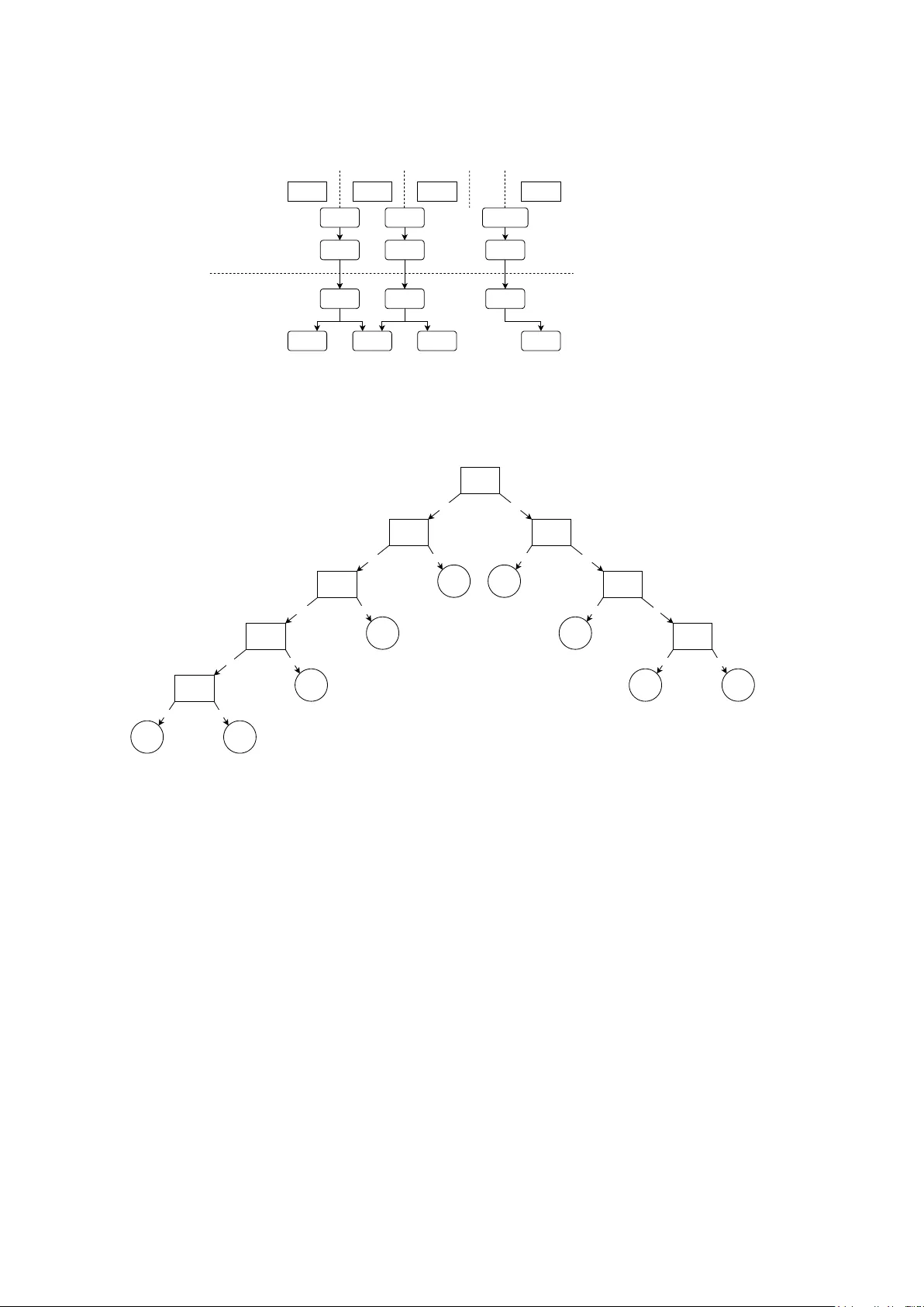
Classifier P o oling for Mo dern Ordinal Classification Noam H. Roten b erg 1 , Andreia V. F aria 2 , Brian Caffo 3* 1 Departmen t of Biomedical Engineering, Whiting Sc ho ol of Engineering, Johns Hopkins Universit y , Baltimore, MD, USA. 2 Departmen t of Radiology , School of Medicine, Johns Hopkins Univ ersity , Baltimore, MD, USA. 3* Departmen t of Biostatistics, Blo om b erg School of Public Health, Johns Hopkins Univ ersity , Baltimore, MD, USA. *Corresp onding author(s). E-mail(s): b caffo1@jh u.edu ; Con tributing authors: noam.roten b erg@y ale.edu ; afaria1@jhmi.edu ; Abstract Ordinal data is widely prev alen t in clinical and other domains, y et there is a lac k of both mo dern, mac hine-learning based metho ds and publicly a v ailable soft ware to address it. In this paper, w e present a mo del-agnostic metho d of ordinal classification, which can apply any non-ordinal classification metho d in an ordinal fashion. W e also provide an op en-source implemen tation of these algorithms, in the form of a Python pac k age. W e apply these mo dels on m ultiple real-world datasets to show their p erformance across domains. W e show that they often outp erform non- ordinal classification methods, especially when the num b er of datap oints is relativ ely small or when there are man y classes of outcomes. This w ork, including the dev elop ed soft w are, facilitates the use of mo dern, more p o werful mac hine learning algorithms to handle ordinal data. Keyw ords: ordinal classification, ordinal regression 1 In tro duction Regression and classification are principal approaches to sup ervised learning. How ev er, certain prediction tasks are not exclusively confined to these approac hes; supervised learning tasks where lab els are finite and ordered can b e framed as ordinal classification (also known as ordinal regression) tasks. Ordinal data is pro duced in v arious settings, including staging in pathology and the Lik ert scale in psychological and consumer surv eys. Ordered logit and ordered probit mo dels are ordinal classification metho ds introduced in the 1970s [ 1 , 2 ]. These mo dels are generalizations of linear mo dels, with mo difications of the logit and probit link functions, resp ectively , that extend their application b ey ond binary data; thresholds on the generalized linear mo del (to facilitate class assignment) are calculated using maximum lik eliho o d estimation. Implemen tations are av ailable in Python [ 3 ] and other languages. The main adv antage of these metho ds is their parsimon y and simplicit y . They require minimal computing resources b ecause their likelihoo d optimization is t ypically conv ex, and they pro vide for clear in terpretation. Ho wev er, these metho ds are often not extended to more p o werful, mo dern mac hine learning classifiers, such as support vector machine and na ¨ ıv e Ba yesian inference. Since computational resources b ecame cheaper and dataset sizes ha ve increased, there is a need for mac hine learning-based ordinal regression metho ds with accessible implemen tation in softw are. 1 When these more p o w erful classifiers are used for ordinal classification tasks, multiclass classifica- tion paradigms that ignore ordinalit y are often used. Classifiers that are inheren tly binary classifiers (whic h cannot nativ ely p erform multiclass classification) can b e adapted for multiclass classification using one vs. rest and one vs. one paradigms. As these metho ds treat class lab els interc hangeably , the metho ds do not take adv antage of p otentially v aluable information enco ded in the ranking of classes. On the other hand, non-categorical regression methods are not ideal for ordinal regression tasks b ecause the numerical representation of the rankings are rarely linear; for example, in cancer grading, the difference betw een stages 1 and 2 should not b e considered the same as the difference b et w een stages 2 and 3. F urthermore, regression metho ds often consider output labels as con tin uous, whic h is not approximately true for lo w num b ers of ordinal categories. Cum ulative and hierarchical ordinal classification are paradigms for po oling machine learning classifiers. These paradigms are model-agnostic, whic h allows for the application of the aforemen- tioned pow erful mac hine learning mo dels that are not nativ ely suited for ordinal classification [ 4 , 5 ]. Ho wev er, to the b est of our knowledge, they w ere not previously implemented in a softw are library , resulting in their underuse and failure to consider certain practical hyperparameters. The purp ose of this paper is to demonstrate no vel approac hes to ordinal regression that allo w users to select any p o werful, mo dern machine learning classifier that b est suits the structure of the dataset. W e demonstrate the capabilities of cum ulative and hierarchical ordinal regression paradigms and also test no vel hyperparameters of these paradigms. T o facilitate the use of these metho ds, an implemen tation is accessible as a Python pac k age (“statlab”), a v ailable on pip (via the command “ !pip install statlab ”), and is compatible with the sklearn-style classifiers. 2 Metho ds 2.1 Mo del-Agnostic Ordinal Classification Algorithms Ob ject-oriented classes were dev elop ed in Python to tak e in an y classifier and perform model- agnostic ordinal classification. DifferenceOrdinalClassifier() with default h yp erparameters p erforms cumulativ e ordinal classification (also called difference-based or subtraction-based ordi- nal classification), and TreeOrdinalClassifier() with default h yp erparameters performs what w e refer to as tree-based or hierarchical ordinal classification. Both metho ds implemen t Algorithm 1 for learning, where classifiers are each assigned a threshold and trained to determine whether sam- ples are ab ov e that threshold, where each threshold corresp onds to a pair of adjacent classes. Each classifier is trained on the entiret y of the dataset, where each outcome v ariable is mapped to a binary outcome, signaling whether an input sample is ab o v e the classifier’s assigned threshold. DifferenceOrdinalClassifier() p erforms A lgorithm 2 for inference, where the probability of a test sample belonging to a giv en class is estimated as the difference b etw een the prediction probabilities of the classifiers assigned to the t w o thresholds adjacent to the giv en class. TreeOrdinalClassifier() implemen ts Algorithm 3 for inference, where the probability of a test sample b elonging to a given class is estimated to b e iterativ ely conditioned up on the prediction probabilities of adjacen t classes, in a path w ay to w ards the b est split index classifier, whic h is assumed to ha ve the most accurate inference. Graphical representations of Algorithms 1 , 2 , and 3 are depicted in Figur es 1a , 1b , and 1c , resp ectiv ely . W e dev elop ed the Python pack age statlab to con tain these classes and deploy ed the pack age on pip. The pac k age p erforms ordinal classification giv en any classifier clf for which the functions clf.fit(X, y) , clf.predict(X) , and clf.predict proba(X) are compatibly defined. This pro- vides functionality with almost all classifiers from the sklearn library [ 6 ]. Note that not all sklearn classifiers enable prediction probabilities, so a simpler metho d is currently implemen ted in statlab ’s BaseOrdinalClassifier() , enabling ordinal classification with truly any base classifier. Note that for simplicity , A lgorithm 1 displays the “even split” method for calculating the b est split index; the default hyperparameter in the soft w are pac k age actually implements the “best classifier” metho d, 2 Algorithm 1: Fitting classifiers for ordinal classification. A binary classifier of t yp e input clf is fit b et ween each adjacen t pair of classes. This algorithm presents the “ev en split” metho d of choosing the b est split index h yp erparameter, but v arious metho ds for choosing this index are compared in Exp eriment 3 below. Input: input clf : binary classification metho d X tr : n umeric features table y tr : n umeric ground-truth lab els of X tr Requiremen t: ( X tr , y tr ) con tains examples for all p ossible ordinal classes. Output: classes : ascending list of unique v alues in y tr classifiers : set of classifiers fit to each threshold b est split idx : index of threshold assumed to b e the b est fit Pro cedure: 1 classes ← ascending list of unique v alues in y tr ; 2 thr esholds ← classes [: − 1]; 3 classifiers ← empty list; 4 foreach class c in thr esholds do 5 clf c ← classifier of type input clf , fit to predict P ( y tr > c ) giv en X tr ; 6 App end clf c to classifiers ; 7 end 8 b est split idx ← arg min i   coun t( y tr > classes [ i ]) − count( y tr ≤ classes [ i ])   ; whic h c ho oses the index with the maximal av erage F1 score across a 4-fold v alidation scheme on the training data. 2.2 Conditional Equiv alence for T ree-based Ordinal Classification F or an ordinal regression task with the n sorted classes c 1 , c 2 , . . . , c n , the b elo w equation holds, whic h is prov ed in the App endix . P ( Y = c x | y ) =                           y − 1 Q a =1 (1 − P ( Y > c a | Y ≤ c a +1 ))  · (1 − P ( Y > c y )) , x = 1 P ( Y > c x − 1 | Y ≤ c x ) ·  y − 1 Q a = x (1 − P ( Y > c a | Y ≤ c a +1 ))  · (1 − P ( Y > c y )) , 1 < x ≤ y P ( Y > c y ) · " x − 1 Q a = y +1 P ( Y > c a | Y > c a − 1 ) # · (1 − P ( Y > c k | Y > c k − 1 )) , y < x < n P ( Y > c y ) · n − 1 Q a = y +1 P ( Y > c a | Y > c a − 1 ) , x = n (1) 2.3 Data Ordinal regression metho ds were compared using data acquired from 6 datasets. Dataset 1 con- tains fetal health data extracted from cardioto cograms of approximately 2,000 patients, whic h are annotated as normal, susp ect pathological, and pathological b y three exp ert obstetricians [ 7 ]. Dataset 2 categorizes cars as unacceptable, acceptable, go od, or very goo d while providing the car’s charac- teristics, suc h as size, price, and comfort [ 8 ]. Dataset 3 categorizes different wines from 1 to 3 based on quality and provides features, such as hue and concentration of v arious chemicals [ 9 ]. Dataset 4 is first-order radiomics data extracted from RetinaMNIST using the Python pack age p yradiomics [ 10 ]; the original RetinaMNIST is a set of 1600 fundus images of diab etic patient retinas, resized to 3x28x28, and graded 1-5 for diab etic retinopathy sev erity [ 11 ]. Dataset 5 is first-order radiomics data 3 Algorithm 2: Inference pro cedure for DifferenceOrdinalClassifier() . Eac h classi- fier is applied to the test sample. A monotonic constraint is applied to the classifier outputs, spreading out ward from the threshold indexed b y the best split index. The test sample prediction probabilities are computed by subtracting the output of adjacen t classifiers. Input: classes : ascending list of unique v alues in y tr classifiers : set of classifiers fit to each threshold b est split idx : index of threshold assumed to b e the b est fit X test : test sample features Output: ˆ y test probs : v ector of prediction probabilities of the test sample for each class in classes ˆ y test : predicted class of the test sample Pro cedure: 1 thr esholds ← classes [: − 1]; 2 clf pr obs ← empt y dictionary; 3 foreach clf, thd pair in classifiers and thr esholds do 4 clf pr obs [ thd ] ← estimation of P( y test > thd ) giv en clf ; 5 end 6 foreach in teger i in the in terv al [ b est split idx , coun t( thr esholds ) − 1) do 7 clf pr obs [ thr esholds [ i + 1]] ← min( clf pr obs [ thr esholds [ i ]] , clf pr obs [ thr esholds [ i + 1]]); 8 end 9 foreach in teger i in the in terv al [1 , b est split idx ], tra versed in rev erse do 10 clf pr obs [ thr esholds [ i − 1]] ← max( clf pr obs [ thr esholds [ i − 1]] , clf pr obs [ thr esholds [ i ]]); 11 end 12 ˆ y test probs ← empt y list; 13 ˆ y test probs [0] ← 1 − clf pr obs [ thr esholds [0]]; 14 ˆ y test probs [1 :] ← vector( clf pr obs )[1 :] − vector( clf pr obs )[: − 1]; 15 ˆ y test ← classes [arg max i ( ˆ y test probs [ i ])] extracted from MNIST, which is a set of 28x28 images of hand-written num b ers b et ween 0-9 [ 12 ]; this is used as a negative con trol, as our metho d is not exp ected to impro ve performance if ordinal- it y is incorp orated into a non-ordinal classification task. Dataset 6 is an estimation of the n umber of rings of an abalone (a t yp e of gastrop od), given v arious b ody characteristics; the n umber of rings is correlated with age [ 13 ]. Datasets 1-3 and 6 w ere randomly split in to training and ev aluation sets with 70% and 30% of the data, resp ectiv ely . F or Datasets 4 and 5, the first 700 training images and first 300 test images w ere used for training and ev aluation, resp ectiv ely . 2.4 Ev aluation In Exp eriment 1 , Logistic Regression, Gaussian Na ¨ ıve Bay es, Support V ector Mac hine, and Gradi- en t Bo osting classifiers were trained on the training sets of Datasets 1-5 through multiple, indep enden t paradigms. The nativ e multiclass me thods were used for Gaussian Na ¨ ıv e Bay es and Gradient Bo osting classifiers; the one vs. rest (O VR) multiclass paradigm was used for Logistic Regression and Support V ector Classification; the sklearn Python pac k age implementation were used for these mo dels [ 6 ]. Difference ordinal classification and tree-based ordinal classification were p erformed for eac h base classifier, according to Algorithms 1-3 abov e. Additionally , an ordered logit mo del and ordered probit mo del were trained from the Python pack age statsmodels [ 3 ]. The default h yp erparameters from eac h pack age were used, to standardize methods. F or each mo del, multiple performance metrics w ere measured on the ev aluation set: accuracy , weigh ted by in verse class size (A W); p olyc horic correlation (PC), which is a correlation metric for ordinal data [ 14 ]; and area under the receiver op erating char- acteristic curve, calculated in a one vs. rest paradigm (A UC OVR). This exp erimen t aims to show the general p erformance of the classification metho ds across m ultiple datasets from v arious domains. 4 Algorithm 3: Inference pro cedure for TreeOrdinalClassifier() . Eac h classifier is applied to the test sample. The test sample prediction probabilities are computed using Equation 1 , where y = b est split idx . Input: classes : ascending list of unique v alues in y tr classifiers : set of classifiers fit to each threshold b est split idx : index of threshold assumed to b e the b est fit X test : test sample features Output: ˆ y test probs : v ector of prediction probabilities of the test sample for each class in classes ˆ y test : predicted class of the test sample Assumptions: 1. F or index i s.t. i < b est split idx : classifiers [ i ] pro vides the estimate P ( Y > c i | Y < c i +1 ) 2. F or index i s.t. i > b est split idx : classifiers [ i ] pro vides the estimate P ( Y > c i | Y > c i − 1 ) Pro cedure: 1 thr esholds ← classes [: − 1]; 2 clf pr obs ← empt y dictionary; 3 foreach clf, thd pair in classifiers and thr esholds do 4 clf pr obs [ thd ] ← prediction probability output of clf on X test ; 5 end 6 ˆ y test probs ← empt y list; 7 foreach i in the interv al [0 , count( classes )) do 8 Calculate ˆ y test probs [ i ] through Equation 1 , given clf pr obs ; 9 end 10 ˆ y test ← classes [arg max i ( ˆ y test probs [ i ])] In Exp eriment 2 , we tested the p erformance of v arious classification metho ds as the n umber of ordinal classes and as dataset size v aried. Classifiers were independently trained on Dataset 6, where the outcome v ariable (num b er of abalone rings) w as grouped into either 3 classes ( < 10 rings, b et ween 10-11 rings, and ≥ 12 rings) or 6 classes: [1, 5), [5, 8), [8, 11), [11, 13), [13, 15), [15, 18) and [18, 29] rings; these groupings w ere formed so that all classes had a substan tial num b er of samples. These t wo trials were conducted twice: first, with models trained on the en tire training set, and second, with mo dels trained on 50% of the training set of Dataset 6. All trials were ev aluated on the same test set. The classifiers trained were the same base models used in Exp eriment 1 . In Exp eriment 3 , w e ev aluated four metho ds for choosing the b est split index, which is an input to A lgorithms 2 and 3 . Equiv alently , we can c ho ose the threshold that corresp onds to this index. One metho d that has b een previously suggested in the literature is arbitrarily choosing the first or last threshold [ 4 ]. Secondly , the most center threshold could b e c hosen. Another metho d, whic h is sho wn in A lgorithm 1 , is to select the threshold where data is most ev enly balanced. Additionally , the threshold with the best classification performance on a held-out v alidation set could b e selected; this could hypothetically minimize incorrect adjustments that are applied to the other mo dels’ outputs in A lgorithm 2 and provide the most robust probability estimation to b e conditioned up on b y the other mo dels’ probabilities in Algorithm 3 . This fourth option is implemen ted in a 4-fold v alidation paradigm during the classifier fitting phase. The four metho ds w ere ev aluated on Dataset 6, using the base mo dels from Exp eriment 1 in difference ordinal classification and tree-based ordinal classification paradigms. The outcome v ariables (num b er of abalone rings) were regroup ed into: [1, 5), [5, 7), [7, 8), [8, 9), [9, 10), [10, 12), [12, 15) and [15, 29]. The purp ose of this manipulation was to distribute the outcome classes non-uniformly , so that the “even split” and “middle index” methods resulted in differen t indices. A summary of the exp erimen ts can b e found in T able 1 . 5 Class 1 Class 2 Class 3 Class n ... Threshold 1 Threshold 2 Threshold n-1 ... Binary classifier 1 Binary classifier 2 Binary classifier {n-1} Figure 1a: Fitting Algorithm 1 on X_train, y_train Figure 1b: Prediction Algorithm 2 on X_test p1 = P(y_test > threshold 1) p2 = P(y_test > threshold 2) p{n-1} = P(y_test > threshold {n-1}) P(y_test = 1) = 1 - p1 P(y_test = 2) = p1 - p2 P(y_test = 3) = p2 - p3 P(y_test = n- 1) = p{n-1} ... ... ... Fitting & Cumulative Prediction T ree-based Prediction classifier j classifier j+1 P(Y > j) classifier j+2 P(Y > j+1 | Y > j) classifier j–1 P(Y ≤ j) classifier j–2 P(Y ≤ j-1 | Y ≤ j) Y=j P(Y > j-1 | Y ≤ j) Y=j+1 P(Y ≤ j+1 | Y > j) classifier n-1 ... Y=j+2 P(Y ≤ j+2 | Y > j) Y=j–1 P(Y > j-2 | Y ≤ j-1) classifier j–3 P(Y ≤ j-2 | Y ≤ j) Y=j–2 P(Y > j-3 | Y ≤ j-2) Y=n-1 P(Y ≤ n-1 | Y > n-2) Y=n P(Y > n-1 | Y > n-2) classifier 1 ... Y=2 P(Y > 1 | Y ≤ 2) Y=1 P(Y ≤ 1 | Y ≤ 2) Figure 1c: Prediction Algorithm 3 on X_test Fig. 1 : 1a : Fitting paradigm for thresholded ordinal classification ( Algorithm 1 ), paired with the difference prediction paradigm (fig. 1b ; Algorithm 2 ). 1c : Prediction paradigm of tree-based ordinal classification ( Algorithm 3 ). T o find P ( Y = i ), multiply all of the conditional probabilities ab o ve the no de Y = i . Equiv alence of this pro duct to P ( Y = i ) is sho wn in the App endix. 3 Results The ra w classifier metrics for Exp eriments 1 , 2 , and 3 are reported in T ables 2 , 3 , and 5 , resp ec- tiv ely . Ev en without hyperparameter tuning, our methods exhibit impro ved p erformance in the ma jority of metrics throughout all tested datasets. In Exp eriment 1 , difference and tree-based ordinal classification mo dels met or outp erformed the nativ e base classifier in 36/48 (75%) and 38/48 (79%) of metrics, resp ectively , across the ordinal datasets 1 through 4. They also frequently outp erformed the ordered logit and probit mo dels. Notably , the tree-based ordinal classification metho d met or out- p erformed the traditional models in all of the metrics in Dataset 2 but p erformed approximately as w ell as them in dataset 3, reinforcing the notion that mo del p erformance is highly dataset-dep enden t. Notably , some traditional mo dels failed to ac hieve b etter-than-c hance p erformance on the RetinaM- NIST radiomics dataset, while none of the difference or tree-based ordinal classification metho ds failed to train on the ordinal datasets (1-4). In Dataset 5, the MNIST radiomics “negativ e control,” tw o of the ordinal mo dels failed to achiev e b etter-than-c hance p erformance, and the other ordinal regression metho ds frequently p erformed 6 Exp erimen t 1 Exp erimen t 2 Exp erimen t 3 T arget comparison Performance of ordinal vs. non-ordinal classifiers across v arious domains Performance of ordinal vs. non-ordinal classifiers as dataset size changes and num b er of classes changes Performance of difference and tree-based ordinal classification as the b est split index hyperparameter changes Datasets Datasets 1-5: fetal health, car quality , wine quality , RetinaMNIST radiomics, MNIST radiomics Dataset 6: abalone rings Dataset 6: abalone rings Classifier t yp es Native multiclass and ordinal classification metho ds for: • Logistic Regression • Gaussian Na ¨ ıve Bayes • Supp ort V ector Classification • Gradient Boosting Classifier Additionally: • Ordered logit mo del • Ordered probit mo del Difference and tree-based ordinal classification only , for: • Logistic Regression • Gaussian Na ¨ ıve Bayes • Supp ort V ector Classification • Gradient Boosting Classifier Metrics W eighted accuracy; polychoric correlation; area under the receiving op erating characteristic curv e, one vs. rest T able 1 : Summary of Exp eriments 1 through 3 . Dataset 1: F etal Health Dataset 2: Car Quality Dataset 3: Wine Quality Dataset 4: RetinaMNIST radiomics Dataset 5: MNIST radiomics (negative control) Method Method Subtype A W PC AUC OVR A W PC AUC OVR A W PC AUC OVR A W PC AUC OVR A W PC AUC OVR Logistic Regression OVR 0.744 0.914 0.925 0.657 0.899 0.963 0.968 0.999 0.998 0.215 0.367 0.637 0.224 0.280 0.690 Ordered logit mo del 0.698 0.911 0.947 0.607 0.909 0.945 0.908 0.999 0.929 * * Difference 0.757 0.906 0.936 0.686 0.907 0.966 0.984 0.999 0.998 0.306 0.594 0.698 0.221 0.294 0.690 T ree-based 0.763 0.912 0.935 0.662 0.913 0.964 0.984 0.999 0.997 0.320 0.604 0.708 0.191 0.325 0.648 Ordered probit mo del 0.702 0.914 0.947 0.586 0.910 0.945 0.908 0.999 0.930 * 0.124 0.126 0.528 Gaussian Na ¨ ıve Bayes Multiclass 0.762 0.831 0.900 0.622 0.894 0.932 0.966 0.999 1.000 0.265 0.383 0.640 0.192 0.238 0.640 Difference 0.775 0.879 0.933 0.754 0.959 0.871 0.966 0.999 0.998 0.248 0.509 0.605 0.192 0.120 0.635 T ree-based 0.775 0.879 0.934 0.708 0.942 0.962 0.966 0.999 0.998 0.285 0.425 0.653 0.178 0.127 0.611 Support V ector OVR 0.612 0.845 0.931 0.812 0.975 0.995 0.605 0.446 0.866 * 0.200 0.202 0.649 Classification Difference 0.716 0.874 0.931 0.930 0.983 0.993 0.668 0.637 0.892 0.292 0.557 0.644 0.111 0.219 0.580 T ree-based 0.692 0.845 0.930 0.909 0.982 0.995 0.598 0.731 0.879 0.299 0.536 0.666 * Gradient Bo osting Multiclass 0.886 0.964 0.984 0.948 0.986 0.998 0.978 0.999 1.000 0.316 0.551 0.638 0.205 0.207 0.682 Classification Difference 0.903 0.973 0.978 0.955 0.986 0.999 0.959 0.999 0.976 0.311 0.531 0.623 0.217 0.266 0.652 T ree-based 0.903 0.973 0.981 0.955 0.986 0.998 0.959 0.999 0.986 0.303 0.482 0.662 0.234 0.308 0.659 T able 2 : Results of Exp eriment 1 ; ev aluation of classification methods, including difference and tree-based ordinal classification, across v arious datasets with ordinal outcome v ariables. Models that failed to train (defined as when the A W was less than c hance) were mark ed b y *. A W = accuracy , w eighted b y inv erse class size; PC = p olyc horic correlation; OVR = one vs. rest; AUC O VR = multi- class area under the receiver operating characteristic curv e, calculated with an OVR paradigm. w orse than the traditional classification metho ds. This suggests that providing ordinal tags to non- ordinal classes decreases classification performance; while MNIST ground-truth lab els are digits 0 through 9, they would more appropriately b e referred to as strings than n umbers. In Exp eriment 2 , man y p erformance metrics decreased as the training set size decreased or as the num b er of outcome classes increased ( T able 3 ). Ho wev er, the decrease in performance of the difference and tree-based ordinal classification methods was generally smaller than that of the other metho ds. T able 4 shows the c hange in p erformance from the full train set, 3-class groupings task to the 50%-reduced train set, 7-class groupings task; the decrease in p erformance was smaller (i.e., less bad) for difference and tree-based ordinal regression in comparison to the native base classifier for 8/12 (67%) and 8/12 (67%) of the metrics, resp ectiv ely . Note that p olyc horic correlation increased as the num b er of outcome classes increased; this may be due to enabling the mo del to provide a higher lev el of gran ularit y with respect to the difference b etw een different samples, even if the exact categorization predicted by the mo del is incorrect. In Exp eriment 3 , using the middle index as the b est split index h yp erparameter outperformed the other indices, achieving the maximum classifier p erformance in 7/24 cases. The other methods follo wed closely b ehind eac h other, with the b est classifier, last index, and even split metho ds ac hiev- ing the maximum metric in 3/24, 3/24, and 1/24 cases, resp ectiv ely . There were multiple instances (7/24) in which all classifiers ac hieved the same performance. 7 F ull training set 50% of training set T raining Paradigm Method Method Subtype A W PC AUC OVR A W PC AUC OVR 3 outcome Logistic Regression OVR 0.594 0.721 0.812 0.590 0.712 0.803 classes Ordered logit mo del 0.571 0.724 0.798 0.576 0.737 0.797 Difference 0.583 0.711 0.806 0.561 0.667 0.796 T ree-based 0.561 0.692 0.802 0.533 0.669 0.790 Ordered probit mo del 0.568 0.727 0.797 0.566 0.735 0.797 Gaussian Na ¨ ıve Bay es Multiclass 0.506 0.578 0.739 0.495 0.565 0.740 Difference 0.483 0.559 0.710 0.482 0.560 0.710 T ree-based 0.480 0.559 0.706 0.486 0.562 0.708 Support V ector Classification OVR 0.565 0.680 0.816 0.503 0.614 0.799 Difference 0.592 0.694 0.809 0.572 0.657 0.797 T ree-based 0.579 0.689 0.811 0.565 0.653 0.798 Gradient Bo osting Classification Multiclass 0.619 0.750 0.828 0.607 0.730 0.817 Difference 0.616 0.751 0.825 0.603 0.732 0.815 T ree-based 0.615 0.761 0.829 0.604 0.738 0.820 7 outcome Logistic Regression OVR 0.241 0.704 0.845 0.236 0.695 0.837 classes Ordered logit mo del 0.296 0.763 0.833 0.299 0.749 0.831 Difference 0.259 0.715 0.844 0.261 0.701 0.833 T ree-based 0.269 0.723 0.841 0.260 0.707 0.829 Ordered probit mo del 0.259 0.750 0.831 0.256 0.740 0.829 Gaussian Na ¨ ıve Bay es Multiclass 0.404 0.646 0.764 0.424 0.653 0.768 Difference 0.394 0.654 0.722 0.398 0.656 0.725 T ree-based 0.383 0.646 0.734 0.383 0.648 0.735 Support V ector OVR 0.242 0.742 0.857 0.236 0.717 0.855 Classification Difference 0.351 0.764 0.826 0.367 0.733 0.817 T ree-based 0.344 0.745 0.857 0.350 0.721 0.855 Gradient Bo osting Multiclass 0.347 0.748 0.837 0.335 0.731 0.818 Classification Difference 0.356 0.768 0.825 0.362 0.747 0.795 T ree-based 0.353 0.768 0.855 0.352 0.739 0.842 T able 3 : Results of Exp eriment 2 ; comparison of classification metho ds, including difference and tree-based ordinal classification, on Dataset 6 (abalone rings), while v arying dataset size and num b er of classes. A W = accuracy , w eighted b y inv erse class size; PC = p olychoric correlation; O VR = one vs. rest; AUC OVR = multi-class area under the receiver op erating characteristic curve, calculated with an OVR paradigm. Method Method Subtype ∆A W ∆PC ∆AUC OVR Logistic Regression OVR -0.358 -0.026 0.025 Ordered logit mo del -0.272 0.025 0.033 Difference -0.322 -0.010 0.027 T ree-based -0.302 0.015 0.028 Ordered probit mo del -0.311 0.012 0.031 Gaussian Na ¨ ıve Bay es Multiclass -0.082 0.074 0.029 Difference -0.084 0.098 0.015 T ree-based -0.097 0.089 0.028 Support V ector Classification OVR -0.329 0.037 0.040 Difference -0.226 0.039 0.008 T ree-based -0.229 0.032 0.044 Gradient Bo osting Classification Multiclass -0.284 -0.018 -0.010 Difference -0.254 -0.004 -0.029 T ree-based -0.264 -0.022 0.013 T able 4 : Results of Exp eriment 2 ; c hange in p erformance from 3 outcome classes on the full dataset to 7 outcome classes on the 50% dataset (i.e., p erformance on 7-class groupings on 50% of the train dataset minus p erformance on 3-class groupings on full train dataset). ∆A W = c hange in accuracy , weigh ted by in verse class size; ∆PC = change in p olyc horic correlation; O VR = one vs. rest; ∆AUC O VR = c hange in multi-class area under the receiver operating characteristic curv e, calculated with an OVR paradigm. 8 Best split index calculation method Even Split Best Classifier (via 4-fold validation)** Last index Middle index Best split index 4 0*** 6 3 Method Method Subtype A W PC AUC OVR A W PC AUC OVR A W PC AUC OVR A W PC AUC OVR Logistic Regression Difference 0.310 0.767 0.824 0.310 0.767 0.824 0.310 0.767 0.824 0.310 0.767 0.824 T ree-based 0.268 0.764 0.813 0.307 0.746 0.815 0.269 0.782 0.816 0.285 0.747 0.814 Gaussian Na ¨ ıve Bayes Difference 0.346 0.689 0.731 0.346 0.689 0.731 0.346 0.689 0.731 0.346 0.689 0.731 T ree-based 0.342 0.684 0.740 0.342 0.685 0.736 0.342 0.683 0.734 0.342 0.685 0.741 Support V ector Difference 0.359 0.762 0.808 0.363 0.763 0.809 0.357 0.759 0.805 0.371 0.764 0.810 Classification T ree-based 0.336 0.757 0.820 0.353 0.760 0.818 0.344 0.774 0.813 0.339 0.759 0.819 Gradient Bo osting Difference 0.376 0.772 0.820 0.381 0.770 0.819 0.378 0.762 0.817 0.381 0.774 0.820 Classification T ree-based 0.366 0.794 0.833 0.380 0.783 0.830 0.369 0.781 0.833 0.373 0.795 0.834 T able 5 : Results of Exp eriment 3 ; comparison of metho ds for choosing the b est split index hyper- param ter on Dataset 6 (abalone rings). The underlined v alues are the maximum for each metric, for each classifier, for each metho d, if the maxim um v alue is unique. A W = accuracy , w eighted by in verse class size; PC = p olychoric correlation; OVR = one vs. rest; A UC OVR = multi-class area under the receiver op erating characteristic curv e, calculated in an OVR paradigm. **Note that the results for this hyperparameter are not the same as in Exp eriment 2 because the v ariables were regrouped, as describ ed in Metho ds: Evaluation . ***Note that the index is dep endent on classifier p erformance, but in this case, the index was 0 for all classifiers. 4 Discussion In this pap er, we ev aluate metho ds for ordinal classification on real-world datasets, including tw o clinical datasets. The improv ed p erformance of ordinal classification ov er non-ordinal classification is marginal for some datasets and large for others, but ov erall sho ws that there is substan tial informa- tion enco ded in the ordinality of the classes that a non-ordinal multiclass paradigm cannot consider. Out of all metrics, ordinal classification usually had greater p olyc horic correlation, as non-ordinal classification do es not hav e any mec hanism to optimize this metric. The tree-based ordinal classi- fication metho d p erformed marginally b etter than the cumulativ e ordinal classification method, so it migh t more robustly represent classifiers’ estimated probabilities. Surprisingly , the choice of the b est split index, might be somewhat arbitrary given the results of Exp eriment 3 . The “middle index” had stronger p erformance ov er the other indices, but additional inv estigation is necessary to deter- mine whether this trend holds true in other datasets. In particular, more inv estigation of the “b est classifier” approach would b e needed before the additional computation time could be deemed jus- tified. Ov erall, these nov el approaches may b e useful when considering the practical limitations of real-w orld data, as some thresholds might hav e few er datapoints than others or may hav e p oorer p erformance for other reasons. In addition, w e pro vide a nov el soft ware implementation, in the Python pack age statlab . Our implemen tation is mo del-agnostic; it is compatible with most sklearn classifiers, and an y other classifier with three functions, of the form: clf.fit(X, y) , clf.predict(X) , and clf.predict proba(X) . The deplo yment of op en-source softw are and the pro vided interoperability allo ws for easy adoption, replication, and testing of metho ds, fulfilling the principles of op en science. A limitation of this work is that it is less useful for deep learning. Neural netw orks ha ve muc h more complicated decision rules that may b e inheren tly adaptable to ordinal classification tasks. Ho wev er, these ordinal classification metho ds are still v ery useful for cases when data is sparse—as emphasized b y Exp eriment 2 —and ma y still allow for using shallo w multi-la yer p erceptrons. An additional limitation is that mo del p erformance is highly dep enden t on the dataset. Shown in Exp eriment 1 , ordinal mo dels p erformed better on some datasets than others, when compared with the non-ordinal mo dels, despite all of the datasets ha ving ordinal outcomes (except for MNIST, the negativ e control). Ho w ever, this limitation is inherent to mac hine learning, and mac hine learning researc hers should alwa ys ev aluate many methodologies to develop a system that b est fits their data. In our implementation, w e provide choices of difference or tree-based ordinal classification, unlimited 9 c hoices of base models, and multiple choices for additional h yp erparameters. Overall, this w ork— including comparisons, softw are implementation, and hyperparameter dev elopmen t—enables simple, in tuitive, but p ow erful modification of classification schemes to improv e mo del p erformance in ordinal regression tasks. Data and Co de Av ailabilit y All data used is publicly accessible. See sources: [ 7 – 9 , 11 – 13 ]. All co de used to pro duce results rep orted in this manuscript are a v ailable in Zeno do: h ttps: //doi.org/10.5281/zeno do.18990527 [ 15 ]. Up dated versions of the softw are may b e found in the statlab gith ub and pypi pack age: https: //gith ub.com/noamrotenberg/statlab , https://p ypi.org/pro ject/statlab . Ac kno wledgemen ts This research was supp orted in part by the National Institute of Deaf and Communication Dis- orders, NIDCD, through R01 DC05375, R01 DC015466, P50 DC014664, the National Institute of Biomedical Imaging and Bio engineering, NIBIB, through P41 EB031771. Comp eting in terests The authors rep ort no competing interests. References [1] McKelvey , R.D., Zav oina, W.: A statistical mo del for the analysis of ordinal lev el dependent v ariables. The Journal of Mathematical So ciology 4 (1), 103–120 (1975) h ttps://doi.org/10.1080/ 0022250X.1975.9989847 [2] McCullagh, P .: Regression models for ordinal data. Journal of the Roy al Statistical So ciety: Series B (Metho dological) 42 (2), 109–127 (1980) h ttps://doi.org/10.1111/j.2517- 6161.1980.tb01109.x [3] Seab old, S., P erktold, J.: statsmo dels: Econometric and statistical mo deling with p ython. In: 9th Python in Science Conference (2010) [4] T utz, G.: Ordinal regression: A review and a taxonomy of mo dels. Wiley In terdisciplinary Reviews: Computational Statistics 14 (2), 1545 (2022) https://doi.org/10.1002/wics.1545 [5] F rank, E., Hall, M.: A simple approach to ordinal classification. In: De Raedt, L., Flac h, P . (eds.) Mac hine Learning: ECML 2001, pp. 145–156. Springer, Berlin, Heidelb erg (2001) [6] Pedregosa, F., V aro quaux, G., Gramfort, A., Michel, V., Thirion, B., Grisel, O., Blondel, M., Prettenhofer, P ., W eiss, R., Dub ourg, V., V anderplas, J., P assos, A., Cournapeau, D., Brucher, M., Perrot, M., Duchesna y , E.: Scikit-learn: Machine learning in Python. Journal of Mac hine Learning Researc h 12 , 2825–2830 (2011) [7] Camp os, D., Bernardes, J.: Cardioto cography. UCI Machin e Learning Rep ository (2000). https: //doi.org/10.24432/C51S4N [8] Bohanec, M.: Car Ev aluation. UCI Mac hine Learning Repository (1988). h ttps://doi.org/10. 24432/C5JP48 [9] Cortez, P ., Cerdeira, A., Almeida, F., Matos, T., Reis, J.: Mo deling wine preferences by data mining from physicochemical prop erties. Decision Supp ort Systems 47 (4), 547–553 (1998) 10 [10] Griethuysen, J.J.M., F edorov, A., Parmar, C., Hosn y , A., Aucoin, N., Naray an, V., Beets-T an, R.G.H., Fillion-Robin, J.-C., Piep er, S., Aerts, H.J.W.L.: Computational Radiomics System to Deco de the Radiographic Phenotype. Cancer Research 77 (21), 104–107 (2017) h ttps://doi.org/ 10.1158/0008- 5472.CAN- 17- 0339 [11] Y ang, J., Shi, R., W ei, D., Liu, Z., Zhao, L., Ke, B., Pfister, H., Ni, B.: Medmnist v2-a large-scale ligh tw eight b enc hmark for 2d and 3d biomedical image classification. Scientific Data 10 (1), 41 (2023) h ttps://doi.org/10.1038/s41597- 022- 01721- 8 [12] LeCun, Y., Bottou, L., Bengio, Y., Haffner, P .: Gradient-based learning applied to do cu- men t recognition. Pro ceedings of the IEEE 86 (11), 2278–2324 (1998) h ttps://doi.org/10.1109/ 5.726791 [13] Nash, W., Sellers, T., T alb ot, S., Ca wthorn, A., F ord, W.: Abalone. UCI Machine Learning Rep ository (1994). h ttps://doi.org/10.24432/C55C7W [14] Olsson, U.: Maxim um likelihoo d e stimation of the p olyc horic correlation coefficient. Psychome- trik a 44 (4), 443–460 (1979) [15] Rotenberg, N., F aria, A., Caffo, B.: Co de for: Classifier Pooling for Mo dern Ordinal Classifica- tion. Zeno do (2026). h ttps://doi.org/10.5281/zeno do.18990527 App endix: Pro of of Equation 1 F or an ordinal regression task with the n sorted classes c 1 , c 2 , . . . , c n , Equation 1 asserts: P ( Y = c x | y ) =                           y − 1 Q a =1 (1 − P ( Y > c a | Y ≤ c a +1 ))  · (1 − P ( Y > c y )) , x = 1 P ( Y > c x − 1 | Y ≤ c x ) ·  y − 1 Q a = x (1 − P ( Y > c a | Y ≤ c a +1 ))  · (1 − P ( Y > c y )) , 1 < x ≤ y P ( Y > c y ) · " x − 1 Q a = y +1 P ( Y > c a | Y > c a − 1 ) # · (1 − P ( Y > c k | Y > c k − 1 )) , y < x < n P ( Y > c y ) · n − 1 Q a = y +1 P ( Y > c a | Y > c a − 1 ) , x = n Pr o of. Given sorted ordinal classes c 1 , c 2 , . . . c i , . . . c j , . . . c k , . . . , c n : Let Y b e the class assignment of a sample of interest, whic h is a random v ariable. Expanding P ( Y = c k ): P ( Y > c j +1 ) = P ( Y > c j +1 , Y > c j ) = P ( Y > c j +1 | Y > c j ) · P ( Y > c j ) P ( Y = c j +1 ) = P ( Y ≤ c j +1 , Y > c j ) = (1 − P ( Y > c j +1 | Y > c j )) · P ( Y > c j ) P ( Y > c j +2 ) = P ( Y > c j +2 , Y > c j +1 ) = P ( Y > c j +2 | Y > c j +1 ) · P ( Y > c j +1 ) = P ( Y > c j +2 | Y > c j +1 ) · P ( Y > c j +1 | Y > c j ) · P ( Y > c j ) Similarly , P ( Y > c k ) = P ( Y > c k , Y > c k − 1 ) = P ( Y > c k | Y > c k − 1 ) · P ( Y > c k − 1 ) = k Q a = j +1 [ P ( Y > c a | Y > c a − 1 )] · P ( Y > c j ) Consequen tly , P ( Y = c k ) = P ( Y > c k − 1 , Y ≤ c k ) = P ( Y ≤ c k | Y > c k − 1 ) · P ( Y > c k − 1 ) = P ( Y > c j ) · k − 1 Q a = j +1 [ P ( Y > c a | Y > c a − 1 )] · (1 − P ( Y > c k | Y > c k − 1 )) Expanding P ( Y = c n ): P ( Y = c n ) = P ( Y > c n − 1 ) = P ( Y > c j ) · n − 1 Q a = j +1 [ P ( Y > c a | Y > c a − 1 )] 11 Expanding P ( Y = c i ): P ( Y ≤ c j − 1 ) = P ( Y ≤ c j − 1 , Y ≤ c j ) = P ( Y ≤ c j − 1 | Y ≤ c j ) · P ( Y ≤ c j ) = (1 − P ( Y > c j − 1 | Y ≤ c j )) · (1 − P ( Y > c j )) P ( Y ≤ c j − 2 ) = P ( Y ≤ c j − 2 , Y ≤ c j − 1 ) = P ( Y ≤ c j − 2 | Y ≤ c j − 1 ) · P ( Y ≤ c j − 1 ) = (1 − P ( Y > c j − 2 | Y ≤ c j − 1 )) · (1 − P ( Y > c j − 1 | Y ≤ c j )) · (1 − P ( Y > c j )) Similarly , P ( Y ≤ c i ) = j − 1 Q a = i [(1 − P ( Y > c a | Y ≤ c a +1 )] · (1 − P ( Y > c j )) Consequen tly , P ( Y = c i ) = P ( Y ≤ c i , Y > c i − 1 ) = P ( Y > c i − 1 | Y ≤ c i ) · P ( Y ≤ c i ) = P ( Y > c i − 1 | Y ≤ c i ) · j − 1 Q a = i [(1 − P ( Y > c a | Y ≤ c a +1 )] · (1 − P ( Y > c j )) Expanding P ( Y = c 1 ): P ( Y = c 1 ) = P ( Y ≤ c 1 ) = j − 1 Q a =1 [(1 − P ( Y > c a | Y ≤ c a +1 )] · (1 − P ( Y > c j )) □ 12