Transmuted logistic-exponential distribution - some new properties, estimation methods and application with infectious disease mortality data

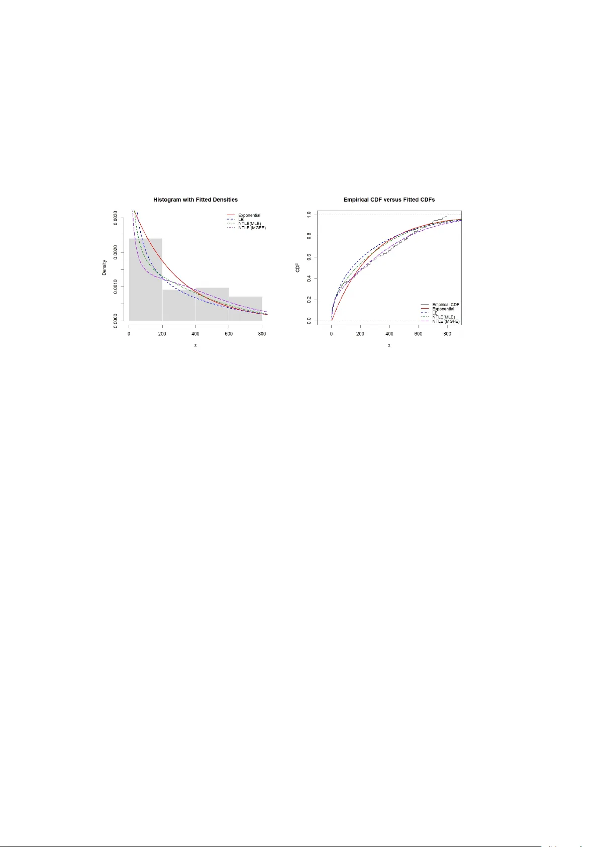
T ransm uted logistic-exp onen tial distribution - some new prop erties, estimation metho ds and application with infectious disease mortalit y data. Isqeel Ogunsola 1,2* , Ab osede Akin tunde 2 , Kehinde Y usuff 2 , Basirat Adetona 2 , and F aheez Ab dulrasaq. 2 1* Departmen t of Mathematics, Universit y of Manchester, United Kingdom. 2 Departmen t of Statistics, F ederal Universit y of Agriculture, Ab eokuta, Nigeria. *Corresp onding author(s). E-mail(s): isqeel.ogunsola@manchester.ac.uk ; Con tributing authors: akin tundeaa@funaab.edu.ng ; yusuffkm@funaab.edu.ng ; sow olabo@funaab.edu.ng ; ab dulrasaqfaheez3@gmail.com ; Abstract Lately , a New T ransm uted Logistic-exponential (NTLE) distribution w as in tro- duced and studied as an extension of the Logistic-Exponential Distribution (LED) with wider applicability in lifetime mo delling. How ever, the maxim um lik eliho o d estimates (MLE) of NTLE are not in closed form, and the consis- tency of the estimates was not examined. F urthermore, some other imp ortan t prop erties of NTLE, namely the Shannon en tropy , R ´ en yi entrop y , sto c hastic ordering, mo de, stress-strength reliability measure, residual life functions (mean and reverse), incomplete moments, Bonferroni and Lorenz curv es are yet to b e deriv ed. Motiv ated b y this, we derived and studied these important prop erties and ev aluated the performance of ten estimation methods (Maxim um Lik eliho od, Momen ts, Least Squares, W eighted Least Squares, Maximum pro duct of Spac- ings, Anderson-Darling, Cramer-v on Mises, percentile estimation, and Maxim um Go odness-of-Fit methods) for NTLE parameters via Monte Carlo sim ulation using bias, mean square error, and ro ot mean square error as ev aluation cri- teria. Real-life infectious mortality data fitted to the distributions show ed that NTLE has a b etter fit compared to its base distributions (Exponential and Logistic-Exp onen tial). This finding contributes v aluable insights for researchers 1 and practitioners when selecting the appropriate estimation metho ds, esp ecially for NTLE and some similar distributions in non-closed form. Keyw ords: Prop erties, Estimation, Non-closed form, Consistency , Monte Carlo, Ev aluation criteria. 1 In tro duction Classical distributions such as the exp onen tial and logistic models are widely used in reliability , surviv al, and lifetime data analysis b ecause of their tractabilit y and in terpretability ( Ogunsola et al. 2026 ). How ever, real data often exhibit comp ound- complex b eha viour that cannot alwa ys b e captured appropriately b y simple mo dels. Consequen tly , the developmen t of more adaptable probability distributions has b ecome an imp ortan t area of researc h in statistics to day . Logisticexp onen tial (LE) distribution combines structural features of the logistic and exp onen tial distributions, pro ducing a more flexible mo del which has a wide v ari- et y of hazard rate b eha viours ( Lan and Leemis 2008 ). Due to its flexibility , the LE distribution has b een applied in mo delling lifetime data with skew ed data and com- plex hazard functions ( Ha j Ahmad and Elnagar 2024 ; Dutta and Ka yal 2024 ). Despite its usefulness, the logisticexp onen tial distribution still lacks sufficien t flexibility in cer- tain situations in volving heavy-tailed or highly skew ed data ( Adesegun et al. 2023 ). T o address such limitations, several extensions of the LE distribution hav e b een pro- p osed in recent y ears ( Genc and Ozbilen 2024 ; Alharbi et al. 2026 ; Mansoor et al. 2019 ; Adesegun et al. 2023 ). Of interest in this study is the new transmuted logistic- exp onen tial (NTLE) distribution, an extension prop osed b y Adesegun et al. ( 2023 ) for modelling lifetime data, whic h has been demonstrated to be useful in reliabil- it y applications. The cumulativ e distribution function (CDF) and the corresp onding probabilit y density function (PDF) of NTLE are given, resp ectiv ely as: G ( y ) = ( e λy − 1) β  1 + δ + ( e λy − 1) β  [ 1 + ( e λy − 1) β ] 2 , y > 0 . (1) and g ( y ) = β λe λy ( e λy − 1) β − 1  (1 + ( e λy − 1) β ) + δ (1 − ( e λy − 1) β )  ( 1 + ( e λy − 1) β ) 3 . (2) also, the hazard and surviv al functions are giv en resp ectiv ely as: h ( y ) = β λe λy ( e λy − 1) β − 1  1 + δ + (1 − δ )( e λy − 1) β  [ 1 + ( e λy − 1) β ] [ 1 + (1 − δ )( e λy − 1) β ] , and ( y ) = 1 + ( e λy − 1) β (1 − δ ) [1 + ( e λy − 1) β ] 2 2 See ( Adesegun et al. 2023 ) for details about NTLE distribution. How ev er, man y imp or- tan t prop erties of NTLE are y et to b e studied. This is one of the gaps among others that this study tends to fill. Alongside the developmen t of new probabilit y models, the problem of parame- ter estimation has received significan t attention in statistical research ( Alsadat et al. 2024 ; Habib et al. 2024 ). Reliable estimation pro cedures are essential for determining whether a proposed distribution can adequately represent observed data. Maxim um lik eliho o d estimation (MLE) ( Fisher 1922 ; Casella and Berger 2002 ) remains the most widely used metho d b ecause of its desirable asymptotic prop erties, including consis- tency and efficiency . Nevertheless, likelihoo d-based estimators ma y sometimes exhibit instabilit y when the lik eliho od equations are difficult to solve n umerically or when sample sizes are small. F or this reason, man y studies inv estigating new probabilit y distributions compare several estimation techniques in order to ev aluate their relative p erformance ( Nombeb e et al. 2023 ; Alabdulhadi and Elgarh y 2024 ). Recent works on newly prop osed lifetime distributions frequen tly compare MLE with alternative estimators suc h as least squares, w eighted least squares, AndersonDarling, Cramrvon Mises, and maximum product of spacings estimators ( Habib et al. 2024 ; Benchiha and Al-Omari 2025 ). Minim um-distance estimators such as the least squares (LSE) and weigh ted least squares (WLSE) estimators are commonly emplo yed when fitting theoretical distri- bution functions to empirical data ( Swain et al. 1988 ). Several recen t studies hav e applied LSE and WLSE estimators in parameter estimation problems inv olving newly prop osed probability mo dels ( Pramanik 2023 ; Onuoha 2023 ). Go odness-of-fit based estimators such as the AndersonDarling and Cramrv on Mises estimators ha ve also b ecome increasingly popular in the statistical literature ( Anderson and Darling 1952 ; Cram ´ er 1928 ). Recent research has demonstrated that AndersonDarling and cramr- v on Mises estimators p erform w ell in parameter estimation studies in volving newly prop osed lifetime distributions ( Habib et al. 2024 ; Pramanik 2023 ). Another es timation technique that has attracted attention in recent studies is the maxim um product of spacings (MPS) estimator ( Luceno 2006 ). Sev eral sim ulation studies hav e shown that MPS estimators often p erform comparably to maximum like- liho od estimators, particularly when dealing with mo derate sample sizes or complex lik eliho o d functions ( Cheng and Amin 1979 ). Bay esian estimation metho ds hav e also gained prominence in recent statistical researc h. Mo dern implemen tations of Bay esian inference t ypically rely on Mark ov chain Monte Carlo algorithms, whic h allo w pos- terior distributions to b e approximated efficiently even when analytical solutions are not a v ailable ( Gelman et al. 2014 ). Although n umerous studies ha ve introduced extensions of logistic-type distribu- tions and examined v arious estimation tec hniques ( Mansoor et al. 2019 ; Ali et al. 2020 ), comprehensiv e inv estigations inv olving a wide range of estimation metho ds for recently introduced transmuted logistic-exp onen tial distributions parameters are not in existence. In particular, no study has compared likelihoo d-based, momen t- based, go odness-of-fit, and Bay esian estimators simultaneously for the new transm uted logistic-exp onen tial t yp e mo del (NTLE). 3 Motiv ated by these gaps in the literature, the present study derived some new imp ortan t properties of NTLE, ev aluated and compared methods for its parameter estimation and examined its improv emen t in mo delling sk ew ed distributions compared to its base distributions (exp onen tial and logistic). Sp ecifically , ten estimation meth- o ds are considered: maximum lik eliho o d estimation, metho d of moments estimation, least squares estimation, w eighted least squares estimation, maxim um product of spac- ings estimation, Ba yesian estimation, AndersonDarling estimation, Cramrvon Mises estimation, p ercentile estimation, and maximum go odness-of-fit estimation. A com- prehensiv e Mon te Carlo simulation study is conducted to ev aluate the performance of these estimators under different sample sizes and parameter v alues. The findings pro vide insight into the relative efficiency and robustness of the comp eting estima- tion pro cedures and demonstrate the p oten tial usefulness of the NTLE distribution for mo delling lifetime data in practical applications. 2 Some New prop erties of NTLE In this section, we present several useful analytical prop erties of the New T ransmuted Logistic exponential (NTLE) distribution not previously studied, namely the Shannon en tropy , R´ en yi entrop y , a stochastic ordering, mode, stress-strength, residual life func- tions (mean and reverse), incomplete momen ts, Bonferroni and Lorenz curves. These prop erties provide insight in to its b ehaviour and practical usefulness in real-world applications. 2.1 Shannon entrop y Shannon en tropy is one of the most widely used measures of uncertain ty in a prob- abilit y distribution. In lifetime and reliability analysis, Shannon entrop y is useful for comparing comp eting distributions in terms of disp ersion and uncertaint y ( Kayid 2023 ; Mac hado 2021 ). A larger entrop y v alue generally indicates greater unpredictability in the underlying lifetime mec hanism. F or a con tinuous random v ariable Y with density function g ( y ), the Shannon en tropy is defined by H ( Y ) = − Z ∞ 0 g ( y ) log g ( y ) dy. (3) Theorem 1 L et Y ∼ N T LE ( λ, β , δ ) with pr ob ability density function g ( y ) = β λe λy ( e λy − 1) β − 1  1 + ( e λy − 1) β  3 h 1 + δ + (1 − δ )( e λy − 1) β i , y > 0 , wher e λ > 0 , β > 0 and − 1 < δ < 1 . Then, the Shannon entropy is in the form H ( Y ) = 2 − log( β λ ) − δ β − j β ,δ − K δ , (4) wher e j β ,δ = Z 1 0 (1 + δ − 2 δ v ) log " 1 +  v 1 − v  1 /β # dv , (5) 4 and K δ = Z 1 0 (1 + δ − 2 δ v ) log(1 + δ − 2 δ v ) dv . (6) F or δ  = 0 , the term K δ has the close d form K δ = (1 + δ ) 2 log(1 + δ ) − (1 − δ ) 2 log(1 − δ ) 4 δ − 1 2 , (7) while, by implic ation, K 0 = 0 . as a r esult, for δ  = 0 , H ( Y ) = 5 2 − log( β λ ) − δ β − j β ,δ − (1 + δ ) 2 log(1 + δ ) − (1 − δ ) 2 log(1 − δ ) 4 δ . (8) Pr o of By definition, H ( Y ) = − Z ∞ 0 g ( y ) log g ( y ) dy . Let, u = ( e λy − 1) β . Then, we hav e; e λy = 1 + u 1 /β , du = β λe λy ( e λy − 1) β − 1 dy , so that g ( y ) dy = 1 + δ + (1 − δ ) u (1 + u ) 3 du. and, g ( y ) = β λ (1 + u 1 /β ) u ( β − 1) /β [1 + δ + (1 − δ ) u ] (1 + u ) 3 . (9) Hence H ( Y ) = − Z ∞ 0 1 + δ + (1 − δ ) u (1 + u ) 3 log " β λ (1 + u 1 /β ) u ( β − 1) /β [1 + δ + (1 − δ ) u ] (1 + u ) 3 # du = − log ( β λ ) − I 1 − β − 1 β I 2 − I 3 + 3 I 4 , (10) where I 1 = Z ∞ 0 1 + δ + (1 − δ ) u (1 + u ) 3 log(1 + u 1 /β ) du, I 2 = Z ∞ 0 1 + δ + (1 − δ ) u (1 + u ) 3 log u du, I 3 = Z ∞ 0 1 + δ + (1 − δ ) u (1 + u ) 3 log  1 + δ + (1 − δ ) u  du, I 4 = Z ∞ 0 1 + δ + (1 − δ ) u (1 + u ) 3 log(1 + u ) du. Using the transformation, v = u 1 + u , u = v 1 − v , du = dv (1 − v ) 2 , 0 < v < 1 . (11) 5 Simplifying, we obtain 1 + δ + (1 − δ ) u (1 + u ) 3 du = (1 + δ − 2 δ v ) dv . (12) Ev aluating I 1 , I 2 , I 3 , I 4 , we hav e; F or I 2 , we hav e log u = log v − log (1 − v ) , I 2 = Z 1 0 (1 + δ − 2 δ v ) log v dv − Z 1 0 (1 + δ − 2 δ v ) log(1 − v ) dv . Using the standard integrals Z 1 0 log v dv = − 1 , Z 1 0 v log v dv = − 1 4 , Z 1 0 log(1 − v ) dv = − 1 , Z 1 0 v log (1 − v ) dv = − 3 4 , w e obtain I 2 = − δ. also, for I 4 , log(1 + u ) = − log(1 − v ) , and I 4 = − Z 1 0 (1 + δ − 2 δ v ) log(1 − v ) dv = 1 − δ 2 . F or I 3 , note that 1 + δ + (1 − δ ) u = 1 + δ − 2 δ v 1 − v , Hence, I 3 = Z 1 0 (1 + δ − 2 δ v ) log(1 + δ − 2 δ v ) dv − Z 1 0 (1 + δ − 2 δ v ) log(1 − v ) dv = K δ + 1 − δ 2 , where K δ is given by ( 6 ). F or δ  = 0, let t = 1 + δ − 2 δ v . Then dt = − 2 δ dv , and K δ = Z 1 0 (1 + δ − 2 δ v ) log(1 + δ − 2 δ v ) dv = 1 2 δ Z 1+ δ 1 − δ t log t dt = 1 2 δ  t 2 2 log t − t 2 4  1+ δ 1 − δ = (1 + δ ) 2 log(1 + δ ) − (1 − δ ) 2 log(1 − δ ) 4 δ − 1 2 . (13) This prov es ( 7 ). The case δ = 0 follows by con tinuit y , giving K 0 = 0. Finally , from ( 12 ), I 1 = Z 1 0 (1 + δ − 2 δ v ) log " 1 +  v 1 − v  1 /β # dv = j β ,δ . (14) Substituting I 1 , I 2 , I 3 , I 4 , into ( 10 ) giv es H ( Y ) = − log( β λ ) − j β ,δ − β − 1 β ( − δ ) −  K δ + 1 − δ 2  + 3  1 − δ 2  . 6 Simplifying further, we obtain H ( Y ) = 2 − log( β λ ) − δ β − j β ,δ − K δ , whic h is ( 4 ). Substituting the closed form ( 7 ) gives ( 8 ). □ R emark 1 When δ = 0, the distribution reduces to the baseline Logistic-Exp onential distribution. Therefore, K 0 = Z 1 0 log(1) dv = 0 . As result, the Shannon en tropy reduces to H ( Y ) = 2 − log( β λ ) − j β , 0 , where j β , 0 = Z 1 0 log " 1 +  v 1 − v  1 /β # dv . This expression represents the Shannon entrop y of the logistic–exp onential distribution with parameters λ and β . The integral j β , 0 do es not admit a closed form and may be ev aluated n umerically for given parameter v alues. 2.2 R ´ en yi entrop y Unlik e the classical Shannon en tropy , R´ enyi en tropy introduces an order parameter that allo ws differen t asp ects of uncertaint y to b e emphasized. It has found applications in signal pro cessing, ecology , and machine learning where the degree of uncertain ty in complex systems m ust b e quantified ( Jizba and Korb el 2019 ). Prop osition 2 L et Y ∼ N T LE ( λ, β , δ ) with λ > 0 , β > 0 , and − 1 < δ < 1 . F or ρ > 0 and ρ  = 1 , the R´ enyi entr opy of Y is define d by H ρ ( Y ) = 1 1 − ρ log  Z ∞ 0 g ( y ) ρ dy  , pr ovide d that the integr al R ∞ 0 g ( y ) ρ dy exists. If ρ = m is an inte ger with m ≥ 2 , then Z ∞ 0 g ( y ) m dy = ( β λ ) m − 1 m − 1 X j =0 m X k =0 m − 1 j ! m k ! (1 + δ ) m − k (1 − δ ) k × B  1 + k + ( m − 1)( β − 1) + j β , 3 m − 1 − k − ( m − 1)( β − 1) + j β  , (15) whenever 1 + k + ( m − 1)( β − 1) + j β > 0 and 3 m − 1 − k − ( m − 1)( β − 1) + j β > 0 for al l j = 0 , 1 , . . . , m − 1 and k = 0 , 1 , . . . , m . Conse quently, H m ( Y ) = 1 1 − m log " ( β λ ) m − 1 m − 1 X j =0 m X k =0 m − 1 j ! m k ! (1 + δ ) m − k (1 − δ ) k 7 × B  1 + k + ( m − 1)( β − 1) + j β , 3 m − 1 − k − ( m − 1)( β − 1) + j β  # . (16) Pr oof By definition, the R´ enyi entrop y of order ρ > 0, ρ  = 1, is H ρ ( Y ) = 1 1 − ρ log  Z ∞ 0 g ( y ) ρ dy  . T o ev aluate the quan tity R ∞ 0 g ( y ) ρ dy , let u = ( e λy − 1) β , 0 < u < ∞ . Then e λy = 1 + u 1 /β , and du = β λe λy ( e λy − 1) β − 1 dy = β λ (1 + u 1 /β ) u ( β − 1) /β dy . Hence, dy = du β λ (1 + u 1 /β ) u ( β − 1) /β . Under this transformation, the densit y becomes g ( y ) = β λ (1 + u 1 /β ) u ( β − 1) /β [1 + δ + (1 − δ ) u ] (1 + u ) 3 . Therefore, g ( y ) ρ = ( β λ ) ρ (1 + u 1 /β ) ρ u ( β − 1) ρ β (1 + δ + (1 − δ ) u ) ρ (1 + u ) − 3 ρ , and so g ( y ) ρ dy = ( β λ ) ρ − 1 u ( β − 1)( ρ − 1) β (1 + u 1 /β ) ρ − 1 (1 + δ + (1 − δ ) u ) ρ (1 + u ) − 3 ρ du. In tegrating both sides ov er (0 , ∞ ) gives Z ∞ 0 g ( y ) ρ dy = ( β λ ) ρ − 1 Z ∞ 0 u ( β − 1)( ρ − 1) β (1 + u 1 /β ) ρ − 1 (1 + δ + (1 − δ ) u ) ρ (1 + u ) − 3 ρ du. No w consider the sp ecial case ρ = m , where m ≥ 2 is an integer. Since m − 1 and m are nonnegativ e in tegers, we may use the finite binomial expansions (1 + u 1 /β ) m − 1 = m − 1 X j =0 m − 1 j ! u j /β , and (1 + δ + (1 − δ ) u ) m = m X k =0 m k ! (1 + δ ) m − k (1 − δ ) k u k . Substituting these into the previous integral yields Z ∞ 0 g ( y ) m dy = ( β λ ) m − 1 Z ∞ 0 u ( β − 1)( m − 1) β   m − 1 X j =0 m − 1 j ! u j /β   m X k =0 m k ! (1 + δ ) m − k (1 − δ ) k u k ! (1 + u ) − 3 m du = ( β λ ) m − 1 m − 1 X j =0 m X k =0 m − 1 j ! m k ! (1 + δ ) m − k (1 − δ ) k Z ∞ 0 u k + ( m − 1)( β − 1)+ j β (1 + u ) − 3 m du. 8 Set a = 1 + k + ( m − 1)( β − 1) + j β . Then a − 1 = k + ( m − 1)( β − 1) + j β , and therefore 3 m − a = 3 m − 1 − k − ( m − 1)( β − 1) + j β . Hence, Z ∞ 0 u k + ( m − 1)( β − 1)+ j β (1 + u ) − 3 m du = Z ∞ 0 u a − 1 (1 + u ) − 3 m du. Using the b eta integral identit y Z ∞ 0 u a − 1 (1 + u ) − ( a + b ) du = B ( a, b ) , a > 0 , b > 0 , with b = 3 m − a = 3 m − 1 − k − ( m − 1)( β − 1) + j β , w e obtain Z ∞ 0 u k + ( m − 1)( β − 1)+ j β (1 + u ) − 3 m du = B  1 + k + ( m − 1)( β − 1) + j β , 3 m − 1 − k − ( m − 1)( β − 1) + j β  , pro vided that 1 + k + ( m − 1)( β − 1) + j β > 0 and 3 m − 1 − k − ( m − 1)( β − 1) + j β > 0 . Therefore, Z ∞ 0 g ( y ) m dy = ( β λ ) m − 1 m − 1 X j =0 m X k =0 m − 1 j ! m k ! (1 + δ ) m − k (1 − δ ) k × B  1 + k + ( m − 1)( β − 1) + j β , 3 m − 1 − k − ( m − 1)( β − 1) + j β  . Finally , substituting this expression into the definition of the R´ en yi entrop y giv es H m ( Y ) = 1 1 − m log " ( β λ ) m − 1 m − 1 X j =0 m X k =0 m − 1 j ! m k ! (1 + δ ) m − k (1 − δ ) k × B  1 + k + ( m − 1)( β − 1) + j β , 3 m − 1 − k − ( m − 1)( β − 1) + j β  # , □ 2.3 Sto c hastic ordering Sto c hastic ordering pro vides a mathematical framework for comparing t wo random v ariables in terms of their magnitude, reliability , or v ariabilit y ( Shak ed and Shanthiku- mar 2007 ; Belzunce 2022 ). If one distribution is sto c hastically larger than another, it tends to pro duce larger v alues and may therefore represent a more reliable system. Prop osition 3 L et Y 1 ∼ N T LE ( λ 1 , β , δ 1 ) , Y 2 ∼ N T LE ( λ 2 , β , δ 2 ) , wher e β > 0 is c ommon to b oth distributions. If λ 1 ≥ λ 2 and δ 1 ≥ δ 2 , then Y 1 ≤ st Y 2 . 9 Pr oof Using the CDF of NTLE in equation 1 , w e can write G r ( y ) = u r ( y ) [1 + δ r + u r ( y )] [1 + u r ( y )] 2 , u r ( y ) =  e λ r y − 1  β , r = 1 , 2 . (17) Let ϕ ( u, δ ) = u (1 + δ + u ) (1 + u ) 2 , u > 0 . Then, G r ( y ) = ϕ ( u r ( y ) , δ r ) . Differen tiating ϕ with resp ect to u and δ gives ∂ ϕ ( u, δ ) ∂ u = 1 + δ + (1 − δ ) u (1 + u ) 3 > 0 , − 1 < δ < 1 , u > 0 , and ∂ ϕ ( u, δ ) ∂ δ = u (1 + u ) 2 > 0 . Hence, ϕ ( u, δ ) is increasing in b oth u and δ . No w, if λ 1 ≥ λ 2 , then for ev ery y > 0, u 1 ( y ) =  e λ 1 y − 1  β ≥  e λ 2 y − 1  β = u 2 ( y ) . T ogether with δ 1 ≥ δ 2 , this gives G 1 ( y ) = ϕ ( u 1 ( y ) , δ 1 ) ≥ ϕ ( u 2 ( y ) , δ 2 ) = G 2 ( y ) , y > 0 . Therefore, G 1 ( y ) ≤ G 2 ( y ) , y > 0 , whic h is equiv alent to Y 1 ≤ st Y 2 . where G r ( y ) = 1 − G r ( y ) □ R emark 2 The ab o ve prop osition sho ws that, for fixed β , the NTLE distribution b ecomes sto c hastically smaller as either λ or δ increases. 2.4 Mo de of the NTLE distribution In lifetime analysis, the mode helps identify the most likely failure time of a comp onen t or system. It is particularly useful when distributions are skew ed, as the mo de may pro vide a more meaningful measure of cen tral tendency than the mean. In practice, the mo de can help engineers and reliability analysts determine the most likely time at whic h failures or even ts o ccur. Theorem 4 L et Y ∼ N T LE ( λ, β , δ ) . Then the mo de of the distribution is char acterise d as fol lows: 1. If 0 < β < 1 , then the density is unb ounde d at the origin and the mo de is y = 0 . 10 2. If β > 1 , then the mo de is the interior p oint y m = 1 λ log(1 + x m ) , wher e x m > 0 is a p ositive r o ot of 1 1 + x + β − 1 x + β (1 − δ ) x β − 1 1 + δ + (1 − δ ) x β − 3 β x β − 1 1 + x β = 0 . (18) 3. If β = 1 , then x m = − 1 + 3 δ 1 − δ . Henc e, if δ < − 1 3 , y m = 1 λ log  − 4 δ 1 − δ  , wher e as for δ ≥ − 1 3 the mo de o c curs at y = 0 . Pr oof Let x = e λy − 1 , x > 0 . Then y = 1 λ log(1 + x ) , and the density b ecomes g ( y ( x )) = β λ (1 + x ) x β − 1 1 + δ + (1 − δ ) x β (1 + x β ) 3 . Since x = e λy − 1 is a strictly increasing function of y , maximizing g ( y ) ov er y > 0 is equiv alent to maximizing g ( y ( x )) ov er x > 0. consider ℓ ( x ) = log g ( y ( x )) . Then ℓ ( x ) = log( β λ ) + log (1 + x ) + ( β − 1) log x + log h 1 + δ + (1 − δ ) x β i − 3 log (1 + x β ) . Differen tiating, dℓ ( x ) dx = 1 1 + x + β − 1 x + β (1 − δ ) x β − 1 1 + δ + (1 − δ ) x β − 3 β x β − 1 1 + x β . Therefore, any interior mo de m ust satisfy dℓ ( x ) dx = 0 , whic h yields the stated nonlinear equation. Next, as y ↓ 0, e λy − 1 ∼ λy , so that g ( y ) ∼ β λ (1 + δ )( λy ) β − 1 . 11 If 0 < β < 1, then g ( y ) → ∞ as y ↓ 0, and hence the mo de is at y = 0. if β > 1, then g ( y ) → 0 as y ↓ 0, so the mode must b e an interior p oin t determined b y the mo dal equation. Finally , for β = 1, the mo dal equation reduces to 1 1 + x + 1 − δ 1 + δ + (1 − δ ) x − 3 1 + x = 0 , that is, − 2 1 + x + 1 − δ 1 + δ + (1 − δ ) x = 0 . Solving for x yields x m = − 1 + 3 δ 1 − δ . Th us x m > 0 if and only if δ < − 1 3 , and in that case y m = 1 λ log(1 + x m ) = 1 λ log  − 4 δ 1 − δ  . When δ ≥ − 1 3 , there is no p ositiv e in terior solution, so the mode o ccurs at the b oundary p oin t y = 0. □ 2.5 Stress-strength reliability The stress-strength reliability parameter measures the probabilit y that a system’s strength exceeds the applied stress, usually expressed as R = p ( Y > X ) where Y represen ts strength and X represents stress. It is used to determine the probabilit y that a comp onen t will p erform satisfactorily under op erational conditions ( Kotz et al. 2003 ; Hassan and Elgarhy 2023 ). The stress–strength reliability for tw o independent random v ariables X and Y is defined as: R = p ( Y < X ) = Z ∞ 0 G Y ( x ) g X ( x ) dx. Prop osition 5 L et X ∼ N T LE ( λ 1 , β 1 , δ 1 ) , Y ∼ N T LE ( λ 2 , β 2 , δ 2 ) , b e indep endent r an- dom variables, wher e X denotes str ength and Y denotes str ess. Then, the stress–str ength r eliability if λ 1 = λ 2 = λ and β 1 = β 2 = β , is R = 1 2 + δ 2 − δ 1 6 . (19) Pr oof By indep endence, R = p ( Y < X ) = Z ∞ 0 G Y ( x ) g X ( x ) dx. F or the NTLE mo del, this b ecomes R = Z ∞ 0 ( e λ 2 x − 1) β 2 h 1 + δ 2 + ( e λ 2 x − 1) β 2 i  1 + ( e λ 2 x − 1) β 2  2 × β 1 λ 1 e λ 1 x ( e λ 1 x − 1) β 1 − 1 h (1 + ( e λ 1 x − 1) β 1 ) + δ 1 (1 − ( e λ 1 x − 1) β 1 ) i  1 + ( e λ 1 x − 1) β 1  3 dx. (20) 12 This gives the general form. No w assume λ 1 = λ 2 = λ and β 1 = β 2 = β . Let u = ( e λx − 1) β . Then du = β λe λx ( e λx − 1) β − 1 dx, and G Y ( x ) = u (1 + δ 2 + u ) (1 + u ) 2 , g X ( x ) dx = 1 + δ 1 + (1 − δ 1 ) u (1 + u ) 3 du. Hence, R = Z ∞ 0 u (1 + δ 2 + u ) [1 + δ 1 + (1 − δ 1 ) u ] (1 + u ) 5 du. Simplifying the numerator u (1+ δ 2 + u ) [1 + δ 1 + (1 − δ 1 ) u ] = (1+ δ 2 )(1+ δ 1 ) u +[(1 + δ 2 )(1 − δ 1 ) + (1 + δ 1 )] u 2 +(1 − δ 1 ) u 3 . Therefore, R = (1 + δ 2 )(1 + δ 1 ) Z ∞ 0 u (1 + u ) 5 du + [(1 + δ 2 )(1 − δ 1 ) + (1 + δ 1 )] Z ∞ 0 u 2 (1 + u ) 5 du + (1 − δ 1 ) Z ∞ 0 u 3 (1 + u ) 5 du. (21) Using Z ∞ 0 u (1 + u ) 5 du = B (2 , 3) = 1 12 , Z ∞ 0 u 2 (1 + u ) 5 du = B (3 , 2) = 1 12 , and Z ∞ 0 u 3 (1 + u ) 5 du = B (4 , 1) = 1 4 , w e obtain R = (1 + δ 2 )(1 + δ 1 ) 12 + (1 + δ 2 )(1 − δ 1 ) + (1 + δ 1 ) 12 + 1 − δ 1 4 . Simplifying, we obtain R = 1 2 + δ 2 − δ 1 6 . This completes the proof. □ R emark 3 When δ 1 = δ 2 , the ab o ve formula reduces to R = 1 2 , whic h is consistent with symmetry when the strength and stress v ariables b elong to the same NTLE mo del. 2.6 Residual life functions Residual life functions are widely used in reliability and surviv al analysis as they describ e the exp ected remaining lifetime of a comp onen t that has survived up to a 13 giv en time ( Louzada et al. 2022 ; Na v arro 2021 ). The mean residual life (MRL) function is m ( t ) = e ( Y − t | Y > t ) = 1 G ( t ) Z ∞ t G ( y ) dy . (22) while the rev ersed residual life (RRL) function is defined as r ( t ) = e ( t − Y | Y ≤ t ) = 1 G ( t ) Z t 0 G ( y ) dy . (23) Prop osition 6 (Mean residual life function) L et Y ∼ N T LE ( λ, β , δ ) the me an r esidual life is m ( t ) = 1 G ( t ) Z ∞ t 1 + (1 − δ ) u ( y ) (1 + u ( y )) 2 dy . (24) Pr oof Let u = ( e λy − 1) β . Then du = β λe λy ( e λy − 1) β − 1 dy . Since e λy = 1 + u 1 /β , w e obtain dy = du β λ (1 + u 1 /β ) u ( β − 1) /β . Hence Z ∞ t G ( y ) dy = Z ∞ u t 1 + (1 − δ ) u (1 + u ) 2 du β λ (1 + u 1 /β ) u ( β − 1) /β , (25) where the surviv al function is G ( y ) = 1 − G ( y ) = 1 + (1 − δ ) u ( y ) (1 + u ( y )) 2 . (26) Therefore m ( t ) = 1 G ( t ) 1 β λ Z ∞ u t 1 + (1 − δ ) u (1 + u ) 2 (1 + u 1 /β ) u ( β − 1) /β du. (27) □ Prop osition 7 (Rev ersed residual life function) The r everse d r esidual life (RRL) function NTLE distribution is given as r ( t ) = 1 G ( t ) Z t 0 u ( y )[1 + δ + u ( y )] (1 + u ( y )) 2 dy . (28) Pr oof Using the transformation u = ( e λy − 1) β , w e ha ve dy = du β λ (1 + u 1 /β ) u ( β − 1) /β . 14 Therefore Z t 0 G ( y ) dy = 1 β λ Z u t 0 u (1 + δ + u ) (1 + u ) 2 (1 + u 1 /β ) u ( β − 1) /β du, (29) □ 2.7 Incomplete moments Incomplete moments describ e the exp ected v alue of a random v ariable o ver a restricted p ortion of its supp ort. In reliability applications, incomplete moments help quan tify the contribution of observ ations b elo w a certain threshold, which is imp ortan t when studying early failures or truncated data. They are also widely used in economic inequalit y measures and insurance risk modelling ( Elgarh y and Almet wally 2022 ). The r th incomplete moment is given b y: µ r ( t ) = e ( Y r 1 { Y ≤ t } ) = Z t 0 y r g ( y ) dy . (30) Prop osition 8 L et Y ∼ N T LE ( λ, β , δ ) . The r th inc omplete moment is given as µ r ( t ) = Z u t 0  1 λ log(1 + u 1 /β )  r 1 + δ + (1 − δ ) u (1 + u ) 3 du, (31) Pr oof By definition; µ r ( t ) = e ( Y r 1 { Y ≤ t } ) = Z t 0 y r g ( y ) dy . (32) Let u = ( e λy − 1) β Then, y = 1 λ log  1 + u 1 /β  and du = β λe λy ( e λy − 1) β − 1 dy Using the PDF in equation 2 and noting that the term β λe λy ( e λy − 1) β − 1 dy also app ears in the density . Hence, the Jacobian cancels the corresp onding component of the densit y , and w e obtain µ r ( t ) = Z  1 λ log(1 + u 1 /β )  r (1 + u ) + δ (1 − u ) (1 + u ) 3 du. Note that (1 + u ) + δ (1 − u ) = 1 + δ + (1 − δ ) u, The integral b ecomes µ r ( t ) = Z u t 0  1 λ log(1 + u 1 /β )  r 1 + δ + (1 − δ ) u (1 + u ) 3 du, (33) □ 15 2.8 Bonferroni and Lorenz curv es Bonferroni and Lorenz curves are used to ols for measuring inequality and concentra- tion within a distribution. The Lorenz curve describ es the cumulativ e proportion of the total v ariable accounted for b y the b ottom fraction of the p opulation, while the Bonferroni curv e provides a related measure of concen tration ( Arshad et al. 2022 ). Prop osition 9 L et F − 1 ( p ) denote the quantile function of the NTLE distribution. The Bonferr oni curve is B ( p ) = 1 pµ Z F − 1 ( p ) 0 y g ( y ) dy , (34) while the L or enz curve is L ( p ) = 1 µ Z F − 1 ( p ) 0 y g ( y ) dy , (35) wher e µ = E ( Y ) . Using the inc omplete first moment µ 1 ( t ) , L ( p ) = µ 1 ( F − 1 ( p )) µ , B ( p ) = µ 1 ( F − 1 ( p )) pµ . (36) F or the NTLE distribution, µ 1 ( F − 1 ( p )) = 1 λ Z u p 0 log(1 + u 1 /β ) 1 + δ + (1 − δ ) u (1 + u ) 3 du, where u p = ( e λF − 1 ( p ) − 1) β . R emark 4 The Bonferroni and Lorenz curves pro vide useful measures of concentration and inequalit y for the NTLE distribution and can b e ev aluated once the incomplete first moment is obtained. 3 Metho ds of parameter estimation for NTLE Let Y 1 , Y 2 , . . . , Y n b e a random sample drawn from a contin uous distribution with probabilit y densit y function g ( y ; θ ) and cumulativ e distribution function G ( xy ; θ ), where θ denotes an unkno wn parameter or a vector of parameters to b e estimated. V arious statistical techniques hav e b een prop osed for estimating such parameters. In this study , ten estimation methods are considered due to their widespread applica- tion in statistical inference and distributional mo deling. The parameters ( λ, β , δ ) are estimated using sev eral estimation techniques describ ed in sections 3.1 - 3.10. 3.1 Maxim um Likelihoo d estimation Maxim um lik eliho od estimation determines parameter v alues that maximize the lik eliho o d of observing the data ( Fisher 1922 ; Casella and Berger 2002 ) 16 The lik eliho o d function for the NTLE distribution based on the observ ed sample is L ( λ, β , δ ) = n Y i =1 g ( y i ; λ, β , δ ) . (37) Substituting the densit y function yields L ( λ, β , δ ) = n Y i =1 β λe λy i ( e λy i − 1) β − 1 [(1 + ( e λy i − 1) β ) + δ (1 − ( e λy i − 1) β )] (1 + ( e λy i − 1) β ) 3 . (38) T aking logarithms, the log-likelihoo d function b ecomes ℓ ( λ, β , δ ) = n ln β + n ln λ + λ n X i =1 y i + ( β − 1) n X i =1 ln( e λy i − 1) + n X i =1 ln h (1 + ( e λy i − 1) β ) + δ (1 − ( e λy i − 1) β ) i − 3 n X i =1 ln h 1 + ( e λy i − 1) β i . The score vector is obtained b y differentiating the log-likelihoo d with resp ect to the parameters ( Adesegun et al. 2023 ): U ( θ ) =  ∂ ℓ ∂ λ , ∂ ℓ ∂ β , ∂ ℓ ∂ δ  T . The lik eliho o d equations are obtained by solving ∂ ℓ ∂ λ = 0 , ∂ ℓ ∂ β = 0 , ∂ ℓ ∂ δ = 0 . (39) These equations do not admit closed-form solutions, numerical pro cedures such as the Newton–Raphson algorithm or quasi-Newton optimization metho ds are emplo yed ( Adesegun et al. 2023 ). 3.1.1 Observ ed Fisher Information Matrix Let i ( θ ) = − ∂ 2 ℓ ∂ θ ∂ θ T denote the observ ed Fisher information matrix. explicitly , i ( θ ) =    − ∂ 2 ℓ ∂ λ 2 − ∂ 2 ℓ ∂ λ∂ β − ∂ 2 ℓ ∂ λ∂ δ − ∂ 2 ℓ ∂ β ∂ λ − ∂ 2 ℓ ∂ β 2 − ∂ 2 ℓ ∂ β ∂ δ − ∂ 2 ℓ ∂ δ∂ λ − ∂ 2 ℓ ∂ δ∂ β − ∂ 2 ℓ ∂ δ 2    . 17 Under asymptotic normal conditions, the maxim um likelihoo d estimator satisfies √ n ( ˆ θ − θ ) → N (0 , i − 1 ( θ )) . Consequen tly , appro ximate confidence interv als for the parameters ma y b e con- structed using ˆ θ i ± z α/ 2 q d V ar ( ˆ θ i ) . 3.2 Metho d of Momen ts estimation The metho d of moments (MME) provides an alternativ e approach for estimating unkno wn parameters b y equating the sample moments with their corresp onding p opulation moments ( Pearson 1894 ). The k th sample moment about the origin is defined as m k = 1 n n X i =1 Y k i , k = 1 , 2 , 3 . (40) Let µ k = e ( Y k ) denote the k th theoretical moment of the NTLE distribution. Then, µ k = e ( Y k ) = Z ∞ 0 y k g ( y ) dy , (41) Using the transformation u = ( e λy − 1) β . Then y = 1 λ log  1 + u 1 /β  , and du = β λe λy ( e λy − 1) β − 1 dy . Hence, µ k = Z ∞ 0  1 λ log(1 + u 1 /β )  k (1 + u ) + δ (1 − u ) (1 + u ) 3 du. (42) Therefore, the first three p opulation moments of the NTLE distribution are µ 1 = Z ∞ 0 1 λ log(1 + u 1 /β ) (1 + u ) + δ (1 − u ) (1 + u ) 3 du, µ 2 = Z ∞ 0  1 λ log(1 + u 1 /β )  2 (1 + u ) + δ (1 − u ) (1 + u ) 3 du, 18 µ 3 = Z ∞ 0  1 λ log(1 + u 1 /β )  3 (1 + u ) + δ (1 − u ) (1 + u ) 3 du. The metho d of momen ts estimators of the parameters ( λ, β , δ ) are obtained b y solving the equations; 1 n n X i =1 Y i = Z ∞ 0 1 λ log(1 + u 1 /β ) (1 + u ) + δ (1 − u ) (1 + u ) 3 du, (43) 1 n n X i =1 Y 2 i = Z ∞ 0  1 λ log(1 + u 1 /β )  2 (1 + u ) + δ (1 − u ) (1 + u ) 3 du, (44) 1 n n X i =1 Y 3 i = Z ∞ 0  1 λ log(1 + u 1 /β )  3 (1 + u ) + δ (1 − u ) (1 + u ) 3 du. (45) Since these equations 43 , 44 and 45 do not give a close form. Hence, the parameter estimates ( ˆ λ, ˆ β , ˆ δ ) are obtained n umerically . 3.3 Least Squares Estimation (LSE) Least squares estimation for distribution parameters is based on minimizing the squared difference b etw een the theoretical distribution function and the empirical distribution function ( Sw ain et al. 1988 ) i.e. n X i =1  G ( y ( i ) ; λ, β , δ ) − i n + 1  2 , (46) where G ( y ( i ) ; λ, β , δ ) is the NTLE cumulativ e distribution function. The least squares ob jective function is therefore given by S ( λ, β , δ ) = n X i =1 " ( e λy ( i ) − 1) β  1 + δ + ( e λy ( i ) − 1) β   1 + ( e λy ( i ) − 1) β  2 − i n + 1 # 2 . Let u i = ( e λy ( i ) − 1) β , i = 1 , 2 , . . . , n. Then G ( y ( i ) ; λ, β , δ ) = u i (1 + δ + u i ) (1 + u i ) 2 , and the ob jective function b ecomes S ( λ, β , δ ) = n X i =1  u i (1 + δ + u i ) (1 + u i ) 2 − i n + 1  2 . W riting r i = u i (1 + δ + u i ) (1 + u i ) 2 − i n + 1 , 19 w e hav e S ( λ, β , δ ) = n X i =1 r 2 i . Hence, ∂ S ∂ θ = 2 n X i =1 r i ∂ r i ∂ θ , θ ∈ { λ, β , δ } . No w, ∂ G ( y ( i ) ; λ, β , δ ) ∂ u i = 1 + δ + (1 − δ ) u i (1 + u i ) 3 , so that ∂ r i ∂ λ = 1 + δ + (1 − δ ) u i (1 + u i ) 3 ∂ u i ∂ λ , ∂ r i ∂ β = 1 + δ + (1 − δ ) u i (1 + u i ) 3 ∂ u i ∂ β , and ∂ r i ∂ δ = u i (1 + u i ) 2 . Since u i = ( e λy ( i ) − 1) β , It follo ws that ∂ u i ∂ λ = β y ( i ) e λy ( i ) ( e λy ( i ) − 1) β − 1 , and ∂ u i ∂ β = ( e λy ( i ) − 1) β log( e λy ( i ) − 1) = u i log( e λy ( i ) − 1) . Therefore, the normal equations for the least squares estimators are n X i =1 r i 1 + δ + (1 − δ ) u i (1 + u i ) 3 β y ( i ) e λy ( i ) ( e λy ( i ) − 1) β − 1 = 0 , (47) n X i =1 r i 1 + δ + (1 − δ ) u i (1 + u i ) 3 u i log( e λy ( i ) − 1) = 0 , (48) and n X i =1 r i u i (1 + u i ) 2 = 0 . (49) These equations are nonlinear in λ , β and δ , closed-form solutions are not av ailable, estimates are obtained n umerically using iterative optimisation metho ds. 20 3.4 W eighted Least Squares Estimation The weigh ted least squares (WLSE) metho d improv es the ordinary least squares esti- mator by assigning differen t weigh ts to the squared deviations b etw een the theoretical and empirical distribution functions ( Swain et al. 1988 ).. This approach accoun ts for the fact that the v ariance of the empirical distribution function dep ends on the order of the observ ations. The WLSE minimizes n X i =1 w i  G ( y ( i ) ; λ, β , δ ) − i n + 1  2 , (50) where w i are weigh ts chosen based on the v ariance of the empirical distribution function. A commonly used w eight function is w i = ( n + 1) 2 ( n + 2) i ( n − i + 1) , i = 1 , 2 , . . . , n. The w eighted least squares ob jectiv e function is therefore defined as W ( λ, β , δ ) = n X i =1 w i " ( e λy ( i ) − 1) β  1 + δ + ( e λy ( i ) − 1) β   1 + ( e λy ( i ) − 1) β  2 − i n + 1 # 2 . F or conv enience, let u i = ( e λy ( i ) − 1) β , i = 1 , 2 , . . . , n. Then G ( y ( i ) ; λ, β , δ ) = u i (1 + δ + u i ) (1 + u i ) 2 , and the w eighted least squares ob jectiv e function b ecomes W ( λ, β , δ ) = n X i =1 w i  u i (1 + δ + u i ) (1 + u i ) 2 − i n + 1  2 . Let r i = u i (1 + δ + u i ) (1 + u i ) 2 − i n + 1 . Then W ( λ, β , δ ) = n X i =1 w i r 2 i . The w eighted least squares estimators ˆ λ W LS E , ˆ β W LS E and ˆ δ W LS E are obtained b y minimizing W ( λ, β , δ ) with resp ect to λ , β and δ . Thus, 21 ∂ W ∂ θ = 2 n X i =1 w i r i ∂ r i ∂ θ , θ ∈ { λ, β , δ } . Using ∂ G ( y ( i ) ; λ, β , δ ) ∂ u i = 1 + δ + (1 − δ ) u i (1 + u i ) 3 , w e obtain ∂ r i ∂ λ = 1 + δ + (1 − δ ) u i (1 + u i ) 3 ∂ u i ∂ λ , ∂ r i ∂ β = 1 + δ + (1 − δ ) u i (1 + u i ) 3 ∂ u i ∂ β , and ∂ r i ∂ δ = u i (1 + u i ) 2 . Since u i = ( e λy ( i ) − 1) β , It follo ws that ∂ u i ∂ λ = β y ( i ) e λy ( i ) ( e λy ( i ) − 1) β − 1 , and ∂ u i ∂ β = u i log( e λy ( i ) − 1) . Therefore, the estimating equations for the w eighted least squares es timators are n X i =1 w i r i 1 + δ + (1 − δ ) u i (1 + u i ) 3 β y ( i ) e λy ( i ) ( e λy ( i ) − 1) β − 1 = 0 , n X i =1 w i r i 1 + δ + (1 − δ ) u i (1 + u i ) 3 u i log( e λy ( i ) − 1) = 0 , and n X i =1 w i r i u i (1 + u i ) 2 = 0 . The weigh ted least squares estimates of the NTLE parameters are obtained n umerically using iterative optimization algorithms. 22 3.5 Maxim um Pro duct of Spacings Estimation (MPS) In this metho d, parameters are estimated by maximizing the geometric mean of spac- ings b et ween successive v alues of the distribution function. ( Cheng and Amin 1979 ; Kurdi et al. 2023 ). This spacing is defined as: D i = G ( y ( i ) ) − G ( y ( i − 1) ) , i = 1 , 2 , . . . , n + 1 , (51) where G ( y (0) ) = 0 , G ( y ( n +1) ) = 1 . The pro duct of spacings is p ( λ, β , δ ) = n +1 Y i =1 D i . Instead of maximizing p , it is con venien t to maximize its logarithm M ( λ, β , δ ) = n +1 X i =1 log D i . Substituting the NTLE distribution function yields D i = ( e λy ( i ) − 1) β  1 + δ + ( e λy ( i ) − 1) β   1 + ( e λy ( i ) − 1) β  2 − ( e λy ( i − 1) − 1) β  1 + δ + ( e λy ( i − 1) − 1) β   1 + ( e λy ( i − 1) − 1) β  2 . The MPS estimators ( ˆ λ M P S , ˆ β M P S , ˆ δ M P S ) are obtained b y solving ∂ M ∂ λ = 0 , ∂ M ∂ β = 0 , ∂ M ∂ δ = 0 . (52) These equations are nonlinear and therefore solv ed numerically . 3.6 Anderson-Darling Estimation The Anderson-Darling estimation metho d is based on minimizing the Anderson- Darling go odness-of-fit statistic b et ween the empirical distribution function and the theoretical distribution function ( Anderson and Darling 1952 ) The Anderson-Darling ob jective function is a ( λ, β , δ ) = − n − 1 n n X i =1 (2 i − 1)  log G ( y ( i ) ) + log  1 − G ( y ( n +1 − i ) )  . (53) The estimates ( ˆ λ ADE , ˆ β ADE , ˆ δ ADE ) are obtained by minimizing a ( λ, β , δ ) with resp ect to the mo del parameters. Substituting the NTLE cum ulative distribution function gives 23 a ( λ, β , δ ) = − n − 1 n n X i =1 (2 i − 1) " log ( e λy ( i ) − 1) β  1 + δ + ( e λy ( i ) − 1) β   1 + ( e λy ( i ) − 1) β  2 ! + log 1 − ( e λy ( n +1 − i ) − 1) β  1 + δ + ( e λy ( n +1 − i ) − 1) β   1 + ( e λy ( n +1 − i ) − 1) β  2 ! # . Again, let u i = ( e λy ( i ) − 1) β , i = 1 , 2 , . . . , n. Then G ( y ( i ) ) = u i (1 + δ + u i ) (1 + u i ) 2 , and 1 − G ( y ( i ) ) = 1 + (1 − δ ) u i (1 + u i ) 2 . Th us the Anderson-Darling ob jectiv e function b ecomes a ( λ, β , δ ) = − n − 1 n n X i =1 (2 i − 1)  log  u i (1 + δ + u i ) (1 + u i ) 2  + log  1 + (1 − δ ) u n +1 − i (1 + u n +1 − i ) 2  . The Anderson-Darling estimators ˆ λ ADE , ˆ β ADE and ˆ δ ADE are obtained b y mini- mizing a ( λ, β , δ ) with resp ect to λ , β and δ . Hence, the estimators satisfy ∂ a ∂ λ = 0 , ∂ a ∂ β = 0 , ∂ a ∂ δ = 0 . Since u i = ( e λy ( i ) − 1) β , the required deriv atives inv olve ∂ u i ∂ λ = β y ( i ) e λy ( i ) ( e λy ( i ) − 1) β − 1 , and ∂ u i ∂ β = u i log( e λy ( i ) − 1) . (54) Also, the Anderson-Darling estimators of the NTLE parameters are obtained n umerically using iterative optimization techniques. 24 3.7 Cramer-v on Mises estimation (CVME) The Cramer-von Mises estimation metho d is another go o dness-of-fit based approach that measures the squared difference b et ween the empirical distribution function and the theoretical distribution function ( Cram ´ er 1928 ). F or ordered observ ations y (1) , y (2) , . . . , y ( n ) , the Cramer-von Mises ob jective func- tion is defined as W 2 ( λ, β , δ ) = 1 12 n + n X i =1  G ( y ( i ) ; λ, β , δ ) − 2 i − 1 2 n  2 , (55) where G ( y ; λ, β , δ ) denotes the cum ulative distribution function of the NTLE dis- tribution. Compared with Anderson-Darling estimation, the Cramr-v on Mises method distributes weigh t more evenly across the entire distribution, rather than emphasizing the tails. Substituting the NTLE cum ulative distribution function gives c ( λ, β , δ ) = 1 12 n + n X i =1 " ( e λy ( i ) − 1) β  1 + δ + ( e λy ( i ) − 1) β   1 + ( e λy ( i ) − 1) β  2 − 2 i − 1 2 n # 2 . (56) The cramr–v on Mises estimators ( ˆ λ C V M E , ˆ β C V M E , ˆ δ C V M E ) are obtained by min- imizing c ( λ, β , δ ) with resp ect to the parameters. Since the resulting equations are nonlinear, n umerical optimization metho ds are required. 3.8 P ercen tile Estimation (PCE) The p ercen tile estimation metho d is based on matching theoretical p ercen tiles of the distribution with sample p ercen tiles obtained from the ordered observ ations ( Kao 1958 ). it is particularly useful in situations where the distribution’s quantile structure is of primary in terest. Let y ( i ) denote the i th ordered observ ation and let the corresponding theoretical cum ulative probability be approximated b y p i = i n + 1 . (57) The theoretical quan tiles satisfy G ( y ( i ) ; λ, β , δ ) = p i , where G ( y ; λ, β , δ ) denotes the cum ulative distribution function of the NTLE dis- tribution. The p ercen tile estimators are obtained by minimizing the sum of squared differences n X i =1  G ( y ( i ) ; λ, β , δ ) − p i  2 . The resulting estimates of the parameters are obtained using n umerical optimiza- tion pro cedures. 25 3.9 Maxim um Go o dness-of-Fit Estimation The maxim um go odness-of-fit estimation (MGFE) approac h estimates the parameters b y minimizing the maximum absolute deviation b et ween the fitted distribution and the empirical distribution ( Luceno 2006 ) The MGFE ob jective function is defined as M ( λ, β , δ ) = max 1 ≤ i ≤ n     G ( y ( i ) ) − i − 0 . 5 n     . (58) Substituting the NTLE cum ulative distribution function yields M ( λ, β , δ ) = max 1 ≤ i ≤ n      ( e λy ( i ) − 1) β  1 + δ + ( e λy ( i ) − 1) β   1 + ( e λy ( i ) − 1) β  2 − i − 0 . 5 n      . (59) The MGFE estimators ( ˆ λ M GF E , ˆ β M GF E , ˆ δ M GF E ) are obtained by minimizing M ( λ, β , δ ) numerically . 3.10 Ba y esian Estimation In the Ba yesian framework, the parameters of the NTLE distribution are treated as random v ariables with prior distributions ( Gelman et al. 2014 ; Dutta and Ka y al 2024 ). Let the join t prior distribution of the parameter vector b e π ( λ, β , δ ) . After observing the data y , the posterior distribution is obtained using Ba yes’ theorem: π ( λ, β , δ | y ) ∝ L ( λ, β , δ ) π ( λ, β , δ ) . The Ba yesian estimates are derived from the p osterior distribution. Under the squared error loss function, the Bay es ian estimator of each parameter is giv en by the p osterior mean ˆ θ B AY E S = e ( θ | y ) . (60) In most cases, the p osterior distribution ma y not hav e a closed-form e xpression; Ba yesian estimates are often obtained using Mark ov c hain Monte Carlo (MCMC) metho ds. 4 Sim ulation Study In this section, we conduct Monte Carlo sim ulation to in vestigate the finitesample per- formance of the parameter estimators discussed in Section 3 for the New T ransmuted Logistic exp onen tial (NTLE) distribution. The ob jectiv e of the simulation exp erimen t w as to assess the relative efficiency and stability of the comp eting estimation metho ds under differen t sample sizes and several parameter v alues Random samples were generated from the NTLE distribution with parameter vec- tor θ = ( λ, β , δ ) via the inv erse transform approach ( Adesegun et al. 2023 ). The parameter v alues w ere fi xed at ( λ = 1 , β = 1 . 5 , δ = 0 . 5) and ( λ = 0 . 5 , β = 1 . 5 , δ = 0 . 2). 26 The simulation exp erimen t was carried out for the sample sizes n = 20 , 50 , 100 , 200 , 500 and 1000 . . F or each generated sample, the parameters ( λ, β , δ ) w ere estimated using the following ten estimation techniques: MLE, MME, LSE, WLSE, MPS, BA YES, ADE, CVME, PCE, and MGFE. Note that for the Bay es metho d, indep enden t Gamma prior distributions are assumed for the parameters λ and β , while a transformation on δ implicitly restricts it to the in terv al ( − 1 , 1). The p osterior sampling is carried out using a random–w alk Metrop olis–Hastings. T o ev aluate the performance of the estimators, the bias, mean squared error and ro ot mean square error were considered. 4.1 Ev aluation Metrics Bias Bias measures the av erage deviation of the estimator from the true parameter v alue. The bias of an estimator ˆ θ is defined as B ias ( ˆ θ ) = 1 R R X r =1 ( ˆ θ r − θ ) , where ˆ θ r denotes the estimate obtained from the r th replication and θ represents the true parameter v alue. Mean Squared Error The mean squared Error (MSE) is defined as M S E ( ˆ θ ) = 1 R R X r =1 ( ˆ θ r − θ ) 2 . The MSE com bines both the v ariance and the bias of an estimator and pro vides a useful measure of o verall estimation accuracy . Ro ot Mean Squared error This is simply the square ro ot of the mean squared error. It is given as: RM S E ( ˆ θ ) = v u u t 1 R R X r =1 ( ˆ θ r − θ ) 2 . 4.2 Sim ulation Results The results of the simulation study provide a comprehensive comparison of the esti- mators in terms of bias and mean squared error across different sample sizes. These findings offer useful insights into the relativ e efficiency and robustness of the comp eting estimation pro cedures for the NTLE distribution. 27 T able 1 Bias, MSE and RMSE of the estimators for the NTLE parameters when n = 20 and ( λ = 1 , β = 1 . 5 , δ = 0 . 5) Bias MSE RMSE Method ˆ λ ˆ β ˆ δ ˆ λ ˆ β ˆ δ ˆ λ ˆ β ˆ δ MLE 0.9523 -0.2396 -0.9278 1.8805 0.1747 1.2133 1.3713 0.4180 1.1015 MME 0.5128 -0.0782 -0.5589 0.6015 0.1629 0.8963 0.7756 0.4036 0.9467 LSE 0.7155 -0.1873 -0.6913 1.0864 0.4108 0.9056 1.0423 0.6409 0.9517 WLSE 0.7166 -0.2381 -0.6127 1.4192 0.1922 0.8350 1.1913 0.4384 0.9138 MPS 0.9855 -0.3886 -0.7462 2.6304 0.2702 1.0398 1.6218 0.5198 1.0197 BA YES 0.5530 -0.1292 -0.5608 0.4002 0.0693 0.3767 0.6326 0.2632 0.6138 ADE 0.6979 -0.2137 -0.6355 1.2973 0.1692 0.8258 1.1390 0.4114 0.9088 CVME 0.7182 -0.0711 -0.7734 0.9302 0.4874 0.9764 0.9644 0.6982 0.9881 PCE 0.7157 -0.3867 -0.5929 1.3915 0.2397 0.8176 1.1796 0.4896 0.9042 MGFE 0.3480 0.0234 -0.4022 0.2181 0.2015 0.2780 0.4670 0.4489 0.5273 T able 2 Bias, MSE and RMSE of the estimators for the NTLE parameters when n = 50 and ( λ = 1 , β = 1 . 5 , δ = 0 . 5). Bias MSE RMSE Method ˆ λ ˆ β ˆ δ ˆ λ ˆ β ˆ δ ˆ λ ˆ β ˆ δ MLE 0.2539 -0.0637 -0.3578 0.2861 0.0339 0.3930 0.5349 0.1840 0.6269 MME 0.3773 -0.1768 -0.5463 0.3755 0.1218 0.7507 0.6128 0.3489 0.8664 LSE 0.2425 -0.0918 -0.3021 0.2594 0.0667 0.3894 0.5093 0.2583 0.6240 WLSE 0.1986 -0.0722 -0.2558 0.2090 0.0512 0.3240 0.4572 0.2263 0.5692 MPS 0.1933 -0.1520 -0.2556 0.2730 0.0542 0.3556 0.5225 0.2329 0.5963 BA YES 0.4203 -0.1301 -0.6022 0.2290 0.0431 0.4324 0.4786 0.2077 0.6576 ADE 0.0956 -0.0378 -0.1203 0.0747 0.0435 0.1824 0.2733 0.2086 0.4271 CVME 0.2492 -0.0474 -0.3112 0.2515 0.0651 0.3996 0.5015 0.2552 0.6322 PCE 0.3623 -0.3230 -0.4232 0.4375 0.1596 0.5526 0.6615 0.3996 0.7433 MGFE 0.2506 -0.0195 -0.4074 0.1218 0.0436 0.3322 0.3491 0.2088 0.5764 The simulation results in T ables 1 – 12 show a clear impro vemen t in estimator p er- formance as the sample size increases. F or b oth parameter settings, the absolute bias, MSE, and RMSE generally decline with increasing n , indicating that all methods b enefit from larger samples. F or the first setting, ( λ, β , δ ) = (1 , 1 . 5 , 0 . 5), the small-sample case in T able 1 shows noticeable bias for most methods, esp ecially in estimating δ . among the comp eting estimators, MGFE p erforms particularly well at n = 20, giving the smallest MSE and RMSE for ˆ λ and ˆ δ , while the Ba yesian metho d p erforms b est for ˆ β . as the sample size increases (T ables 2 – 6 ), the estimators b ecome more stable. In the larger samples, MLE, MPS, PCE, and MGFE are generally the most comp etitiv e, with MPS and PCE sho wing esp ecially strong p erformance at n = 500 and n = 1000. A similar pattern is observed for the second setting, ( λ, β , δ ) = (0 . 5 , 1 . 5 , 0 . 2), rep orted in T ables 7 – 12 . at n = 20, MGFE again stands out, particularly for ˆ λ and ˆ δ , while the Bay esian estimator remains comp etitiv e. F or mo derate and large sample sizes, no single method dominates uniformly across all three parameters, but MGFE, WLSE, MLE, and Bay esian estimation rep eatedly show go od ov erall performance. In 28 T able 3 Bias, MSE and RMSE of the estimators for the NTLE parameter when n = 100 and ( λ = 1 , β = 1 . 5 , δ = 0 . 5) Bias MSE RMSE Method ˆ λ ˆ β ˆ δ ˆ λ ˆ β ˆ δ ˆ λ ˆ β ˆ δ MLE 0.3204 -0.1300 -0.5469 0.2461 0.0479 0.6101 0.4961 0.2189 0.7811 MME 0.3934 -0.1885 -0.6476 0.3629 0.0873 0.8210 0.6024 0.2954 0.9061 LSE 0.3062 -0.1158 -0.4653 0.3251 0.0718 0.5430 0.5702 0.2680 0.7369 WLSE 0.3324 -0.1376 -0.5286 0.3219 0.0656 0.6133 0.5674 0.2561 0.7831 MPS 0.3341 -0.2081 -0.4899 0.3638 0.0857 0.6845 0.6032 0.2928 0.8273 BA YES 0.3675 -0.1484 -0.6163 0.1675 0.0346 0.4717 0.4093 0.1860 0.6868 ADE 0.4046 -0.1777 -0.6214 0.3887 0.0808 0.7736 0.6235 0.2842 0.8795 CVME 0.3385 -0.0969 -0.5391 0.3197 0.0681 0.5768 0.5654 0.2609 0.7595 PCE 0.1281 -0.1890 -0.2247 0.1581 0.0615 0.3490 0.3977 0.2480 0.5908 MGFE 0.2993 -0.0844 -0.5713 0.1411 0.0281 0.5283 0.3757 0.1675 0.7269 T able 4 Bias, MSE and RMSE of the estimators for the NTLE parameters when when n = 200 and ( λ = 1 , β = 1 . 5 , δ = 0 . 5) Bias MSE RMSE Method ˆ λ ˆ β ˆ δ ˆ λ ˆ β ˆ δ ˆ λ ˆ β ˆ δ MLE 0.2676 -0.1233 -0.3961 0.2190 0.0465 0.4367 0.468 0.2156 0.6609 MME 0.1754 -0.1591 -0.2117 0.2200 0.0549 0.3769 0.4690 0.2344 0.614 LSE 0.3240 -0.1266 -0.4566 0.2948 0.0595 0.4690 0.5429 0.2440 0.6849 WLSE 0.3801 -0.1623 -0.4876 0.4297 0.0824 0.5946 0.6555 0.2870 0.7711 MPS 0.1945 -0.1606 -0.2492 0.2205 0.0592 0.4233 0.4696 0.2432 0.6506 BA YES 0.3366 -0.1559 -0.4939 0.1939 0.0418 0.3850 0.4404 0.2046 0.6205 ADE 0.3944 -0.1626 -0.5104 0.4366 0.0834 0.6068 0.6608 0.2888 0.7790 CVME 0.4405 -0.1619 -0.5599 0.4957 0.0930 0.6652 0.7041 0.3050 0.8156 PCE -0.0022 -0.1621 0.0322 0.0673 0.0439 0.1628 0.2595 0.2096 0.4035 MGFE 0.2869 -0.0807 -0.4880 0.1289 0.0272 0.3477 0.3591 0.1649 0.5897 particular, MGFE giv es some of the smallest MSE and RMSE v alues in T ables 8 , 10 , 11 , and 12 . 29 T able 5 Bias, MSE and RMSE of the estimators for the NTLE parameters when n = 500 and ( λ = 1 , β = 1 . 5 , δ = 0 . 5) Bias MSE RMSE Method ˆ λ ˆ β ˆ δ ˆ λ ˆ β ˆ δ ˆ λ ˆ β ˆ δ MLE 0.1334 -0.0472 -0.2224 0.0775 0.0116 0.1896 0.2784 0.1078 0.4354 MME 0.2363 -0.1403 -0.3594 0.1748 0.0384 0.3838 0.4180 0.1959 0.6195 LSE 0.3124 -0.1058 -0.4661 0.2443 0.0368 0.4432 0.4943 0.1918 0.6657 WLSE 0.2031 -0.0630 -0.3345 0.1137 0.0159 0.2584 0.3372 0.1262 0.5083 MPS 0.0532 -0.0678 -0.0641 0.0739 0.0132 0.1757 0.2718 0.1150 0.4191 BA YES 0.2705 -0.1031 -0.4236 0.1193 0.0196 0.2800 0.3454 0.1398 0.5292 ADE 0.2546 -0.0876 -0.3891 0.1843 0.0298 0.3621 0.4293 0.1725 0.6017 CVME 0.3685 -0.1248 -0.5205 0.3289 0.0528 0.5423 0.5735 0.2298 0.7364 PCE 0.0251 -0.1083 -0.0038 0.0759 0.0250 0.1547 0.2755 0.1582 0.3933 MGFE 0.2464 -0.0597 -0.4204 0.1059 0.0150 0.2830 0.3254 0.1225 0.5319 T able 6 Bias, MSE and RMSE of the estimators for the NTLE parameters when n = 1000 and ( λ = 1 , β = 1 . 5 , δ = 0 . 5). Bias MSE RMSE Method ˆ λ ˆ β ˆ δ ˆ λ ˆ β ˆ δ ˆ λ ˆ β ˆ δ MLE 0.0708 -0.0129 -0.1324 0.0229 0.0035 0.0865 0.1514 0.0594 0.2941 MME 0.1657 -0.1040 -0.2646 0.1109 0.0222 0.3024 0.3331 0.1491 0.5499 LSE 0.3640 -0.1139 -0.5297 0.3114 0.0465 0.5497 0.5580 0.2157 0.7414 WLSE 0.0909 -0.0187 -0.1604 0.0340 0.0046 0.1139 0.1843 0.0677 0.3374 MPS 0.0337 -0.0397 -0.0339 0.0553 0.0122 0.1299 0.2352 0.1104 0.3604 BA YES 0.1540 -0.0455 -0.2615 0.0586 0.0082 0.1562 0.2422 0.0903 0.3952 ADE 0.0771 -0.0198 -0.1340 0.0330 0.0046 0.1102 0.1817 0.0681 0.3320 CVME 0.3641 -0.1114 -0.5305 0.3106 0.0461 0.5493 0.5573 0.2146 0.7412 PCE 0.0562 -0.1004 -0.0593 0.0908 0.0249 0.1913 0.3013 0.1576 0.4374 MGFE 0.2374 -0.0287 -0.4304 0.0818 0.0084 0.2576 0.2860 0.0915 0.5076 T able 7 Bias, MSE and RMSE of the estimators for the NTLE parameters when n = 20 and ( λ = 0 . 5 , β = 1 . 5 , δ = 0 . 2) Bias MSE RMSE Method ˆ λ ˆ β ˆ δ ˆ λ ˆ β ˆ δ ˆ λ ˆ β ˆ δ MLE 0.2636 -0.1702 -0.4939 0.2195 0.1199 0.5446 0.4685 0.3463 0.7380 MME 0.1999 -0.0444 -0.4571 0.0966 0.1894 0.6232 0.3109 0.4352 0.7894 LSE 0.2486 -0.1931 -0.4041 0.1687 0.4080 0.5820 0.4108 0.6387 0.7629 WLSE 0.2464 -0.2403 -0.3180 0.2306 0.1925 0.5578 0.4802 0.4387 0.7469 MPS 0.3086 -0.3463 -0.3547 0.3930 0.2333 0.5642 0.6269 0.4830 0.7512 BA YES 0.2627 -0.1830 -0.3907 0.0984 0.0937 0.2087 0.3136 0.3060 0.4569 ADE 0.2584 -0.2402 -0.4145 0.2107 0.1756 0.6010 0.4591 0.4191 0.7752 CVME 0.2950 -0.1123 -0.5694 0.1828 0.5034 0.706 0.4275 0.7095 0.8402 PCE 0.2658 -0.4007 -0.3664 0.2270 0.2615 0.5640 0.4765 0.5113 0.7510 MGFE 0.1117 -0.0060 -0.2107 0.0266 0.1809 0.1674 0.1631 0.4253 0.4091 30 T able 8 Bias, MSE and RMSE of the estimators for the NTLE parameters when n = 50 and ( λ = 0 . 5 , β = 1 . 5 , δ = 0 . 2) Bias MSE RMSE Method ˆ λ ˆ β ˆ δ ˆ λ ˆ β ˆ δ ˆ λ ˆ β ˆ δ MLE 0.0761 -0.0826 -0.1389 0.0610 0.0471 0.3322 0.2469 0.2170 0.5763 MME 0.1002 -0.1487 -0.2653 0.0488 0.1106 0.4974 0.2209 0.3325 0.7053 LSE 0.0487 -0.0980 -0.0519 0.0386 0.0666 0.2927 0.1964 0.2580 0.5410 WLSE 0.0209 -0.0731 0.0391 0.0322 0.0504 0.2581 0.1795 0.2244 0.5080 MPS 0.0235 -0.1459 0.0257 0.0444 0.0533 0.2883 0.2107 0.2309 0.5370 BA YES 0.1766 -0.1772 -0.4550 0.0441 0.0603 0.2734 0.2099 0.2457 0.5229 ADE 0.0185 -0.0677 0.0398 0.0306 0.0447 0.2567 0.1749 0.2115 0.5067 CVME 0.0729 -0.0597 -0.1605 0.0359 0.0641 0.2858 0.1894 0.2531 0.5346 PCE 0.0641 -0.3044 -0.0466 0.0642 0.1507 0.4208 0.2534 0.3882 0.6487 MGFE 0.0665 -0.0373 -0.1823 0.0223 0.0398 0.1989 0.1492 0.1996 0.4460 T able 9 Bias, MSE and RMSE of the estimators for the NTLE parameter when n = 100 and ( λ = 0 . 5 , β = 1 . 5 , δ = 0 . 2) Bias MSE RMSE Method ˆ λ ˆ β ˆ δ ˆ λ ˆ β ˆ δ ˆ λ ˆ β ˆ δ MLE 0.0431 -0.1028 -0.1110 0.0264 0.0261 0.2409 0.1626 0.1616 0.4908 MME 0.1418 -0.2956 -0.2914 0.0931 0.1625 0.6875 0.3052 0.4031 0.8291 LSE 0.1407 -0.2140 -0.3596 0.0695 0.0935 0.4400 0.2636 0.3059 0.6633 WLSE 0.0815 -0.1569 -0.1864 0.0515 0.0607 0.3283 0.2269 0.2464 0.5729 MPS 0.0199 -0.1578 -0.0074 0.0316 0.0400 0.2979 0.1779 0.2000 0.5458 BA YES 0.1063 -0.1627 -0.2455 0.0319 0.0462 0.1504 0.1785 0.2148 0.3878 ADE 0.1919 -0.2433 -0.4322 0.1220 0.1293 0.5801 0.3493 0.3595 0.7616 CVME 0.1633 -0.2195 -0.4389 0.0748 0.0920 0.5096 0.2735 0.3033 0.7138 PCE 0.0305 -0.2373 0.0365 0.0571 0.1014 0.3331 0.2389 0.3184 0.5771 MGFE 0.0681 -0.1066 -0.2184 0.0220 0.0376 0.1808 0.1484 0.1940 0.4252 T able 10 Bias, MSE and RMSE of the estimators for the NTLE parameters when n = 200 and ( λ = 0 . 5 , β = 1 . 5 , δ = 0 . 2) Bias MSE RMSE Method ˆ λ ˆ β ˆ δ ˆ λ ˆ β ˆ δ ˆ λ ˆ β ˆ δ MLE 0.0772 -0.1297 -0.2010 0.0319 0.0495 0.2897 0.1787 0.2225 0.5383 MME 0.0985 -0.1728 -0.2131 0.0582 0.0726 0.4008 0.2411 0.2694 0.6331 LSE 0.0688 -0.1152 -0.1849 0.0230 0.0452 0.2191 0.1518 0.2127 0.4681 WLSE 0.0555 -0.1164 -0.1281 0.0255 0.0459 0.2500 0.1596 0.2143 0.5000 MPS 0.0760 -0.1915 -0.1236 0.0508 0.0825 0.4317 0.2253 0.2872 0.6570 BA YES 0.1230 -0.1796 -0.3221 0.0346 0.0544 0.2508 0.1860 0.2332 0.5008 ADE 0.1335 -0.1882 -0.2806 0.0774 0.1009 0.4594 0.2781 0.3177 0.6778 CVME 0.0694 -0.1034 -0.1893 0.0224 0.0429 0.2162 0.1498 0.2072 0.4649 PCE -0.0427 -0.1391 0.2286 0.0163 0.0340 0.2596 0.1276 0.1845 0.5095 MGFE 0.0669 -0.0931 -0.2255 0.0132 0.0283 0.1657 0.1150 0.1682 0.4071 31 T able 11 Bias, MSE and RMSE of the estimators for the NTLE parameters when n = 500 and ( λ = 0 . 5 , β = 1 . 5 , δ = 0 . 2) Bias MSE RMSE Method ˆ λ ˆ β ˆ δ ˆ λ ˆ β ˆ δ ˆ λ ˆ β ˆ δ MLE 0.0672 -0.0907 -0.2069 0.0209 0.0226 0.2093 0.1445 0.1503 0.4575 MME 0.1183 -0.1915 -0.3054 0.0518 0.0688 0.4254 0.2277 0.2624 0.6522 LSE 0.0983 -0.1351 -0.2362 0.0467 0.0562 0.3239 0.2160 0.2370 0.5692 WLSE 0.0379 -0.0681 -0.1005 0.0145 0.0177 0.1449 0.1206 0.1331 0.3807 MPS 0.0349 -0.1007 -0.0670 0.0220 0.0244 0.2486 0.1483 0.1563 0.4986 BA YES 0.0981 -0.1347 -0.2710 0.0246 0.0310 0.2067 0.1569 0.1761 0.4546 ADE 0.0730 -0.1054 -0.1846 0.0310 0.0402 0.2503 0.1762 0.2005 0.5003 CVME 0.1257 -0.1558 -0.3030 0.0595 0.0723 0.3933 0.2440 0.2690 0.6272 PCE -0.0149 -0.1024 0.1386 0.0213 0.0264 0.2455 0.1458 0.1623 0.4955 MGFE 0.0532 -0.0791 -0.1487 0.0165 0.0248 0.1674 0.1283 0.1573 0.4092 T able 12 Bias, MSE and RMSE of the estimators for the NTLE parameters when n = 1000 and ( λ = 0 . 5 , β = 1 . 5 , δ = 0 . 2) Bias MSE RMSE Method ˆ λ ˆ β ˆ δ ˆ λ ˆ β ˆ δ ˆ λ ˆ β ˆ δ MLE 0.0743 -0.0992 -0.2027 0.0304 0.0385 0.2852 0.1744 0.1962 0.5341 MME 0.0674 -0.1017 -0.2122 0.0216 0.0257 0.2289 0.1468 0.1604 0.4784 LSE 0.0962 -0.1218 -0.2165 0.0508 0.0627 0.3631 0.2254 0.2503 0.6026 WLSE 0.0623 -0.0917 -0.1395 0.0341 0.0397 0.2788 0.1846 0.1992 0.5280 MPS 0.0831 -0.1356 -0.1996 0.0407 0.0518 0.3851 0.2019 0.2276 0.6205 BA YES 0.0677 -0.1007 -0.1845 0.0200 0.0250 0.1849 0.1415 0.1581 0.4301 ADE 0.0639 -0.0909 -0.1281 0.0390 0.0460 0.2838 0.1976 0.2145 0.5327 CVME 0.1123 -0.1269 -0.2805 0.0520 0.0634 0.3669 0.2280 0.2519 0.6058 PCE 0.0038 -0.0819 0.0818 0.0292 0.0308 0.2635 0.1708 0.1754 0.5133 MGFE 0.0619 -0.0650 -0.1925 0.0171 0.0242 0.1745 0.1310 0.1557 0.4177 32 5 Application with infectious diseases death data In this section, the practical usefulness of the prop osed New T ransmuted Logistic- exp onen tial (NTLE) distribution is illustrated b y means of a real dataset. The data used is the deaths due to COVID-19 in Egypt in 2020 ( El-Monsef et al. 2021 ). The main ob jectiv e is to assess the ability of the NTLE mo del to describ e the observ ed data and to compare its p erformance with its base distributions, namely , the exp onen tial and logistic-exp onen tial (Le) distribution. 5.1 Comparison of NTLE with base distributions Here, for the mortality data, the NTLE parameters were MLE and MGFE estimation metho ds, while the comp eting models w ere fitted b y maximum lik eliho o d estima- tion. T o examine the relativ e adequacy of the fitted mo dels, the follo wing criteria w ere considered: the log-lik eliho od v alue, Ak aike information criterion (AIC), Ba yesian information criterion (BIC), corrected Ak aike information criterion (CAIC), Hannan- Quinn information criterion (HQIC), the Kolmogoro v-Smirnov (K–S) statistic, and the corresp onding p -v alue. Let ℓ ( ˆ Φ) denote the maximized log-likelihoo d, p the num b er of estimated param- eters, and m the sample size. Then, the AIC, BIC, CAIC, HQIC, and K-S statistics are defined, resp ectiv ely as: AI C = − 2 ℓ ( ˆ Φ) + 2 p. B I C = − 2 ℓ ( ˆ Φ) + p log m. C AI C = − 2 ℓ ( ˆ Φ) + p (log m + 1) . H QI C = − 2 ℓ ( ˆ Φ) + 2 p log(log m ) . D m = sup y    G m ( y ) − G ( y ; ˆ Φ)    , where G m ( y ) is the empirical distribution function and G ( y ; ˆ θ ) is the fitted cum ulative distribution function. A smaller v alue of D m indicates closer agreement b et ween the fitted mo del and the observed data. The corresp onding p -v alue is obtained from the Kolmogorov-Smirno v test and is used to assess the adequacy of the fitted distribution. A larger p -v alue suggests that the fitted mo del is more consistent with the observed data. The fitted mo dels were also examined graphically using the histogram with fitted density curv es and the empirical cum ulative distribution function plotted against the fitted cumulativ e distribution functions. 33 T able 13 parameter estimates and goo dness-of-fit measures for the fitted mo dels. Model ˆ α ˆ β ˆ λ loglik AIC BIC CAIC HQIC K-S p -v alue exponential 0.0036 -510.1720 1022.3440 1024.6878 1025.6878 1023.2815 0.1408 0.0945 Le 0.0050 0.6571 -502.8429 1009.6857 1014.3733 1016.3733 1011.5607 0.1286 0.1564 NTLE (MLE) 0.0085 0.4732 -0.5830 -500.4086 1006.8171 1013.8485 1016.8485 1009.6296 0.0967 0.4669 NTLE (MGF) 0.0134 0.2935 -0.9272 -500.7561 1007.5122 1014.5436 1017.5436 1010.3247 0.0791 0.7216 34 T able 13 presen ts the parameter estimates and go o dness-of-fit statistics for the comp eting mo dels fitted to the data. Although NTLE estimated through MLE sho ws the smallest AIC v alue, the NTLE mo del estimated through the MGFE method yields the smallest Kolmogorov-Smirno v statistic and the largest p -v alue, indicating a closer agreemen t b et ween the fitted distribution and the empirical data. In all, the re sults suggest that incorporating the additional flexibilit y of the NTLE distribution allows the mo del to capture the underlying structure of the data more effectively than the base alternativ es. Fig. 1 Histogram of COVID - 19 deaths in Egypt with fitted density functions of the com- peting mo dels. Fig. 2 Empirical cumulativ e distribution func- tion and fitted cumulative distribution functions of the competing mo dels. The histogram with the fitted distributions is shown in Figure 1 while the plot of the empirical cumulativ e distribution function and fitted cumulativ e distribution func- tions of the mo dels is giv en in Figure 2 . The visual comparisons shown in Figures 1 and 2 further supp ort the adequacy of the fitted NTLE mo del. The fitted NTLE(MGFE) densit y follo ws the shap e of the histogram closely , while the fitted cumulativ e dis- tribution function tracks the empirical CDF more accurately than other compared mo dels. 6 Discussion of Results The simulation results suggest that MGFE is a strong and reliable choice, esp ecially in small and moderate samples, while MLE and a few alternative metho ds b ecome increasingly competitive as the sample size gro ws. This findings also confirm that estimation of the transm utation parameter δ is generally more difficult than estimation of λ and β , particularly in smaller samples. In addition, this study also pro vides useful insight into the p erformance of the New T ransmuted Logistic-exp onen tial (NTLE) distribution when applied to 35 real lifetime data. The NTLE mo del was fitted using the maximum goo dness-of- fit estimation (MGFE) and MLE metho d, while the base mo dels (Exp onen tial and Logistic-Exp onen tial) distributions were estimated using maxim um likelihoo d pro ce- dures and compared using sev eral information criteria and go odness-of-fit statistics (loglik eliho o d, AIC, BIC, CAIC, HQIC, and K-S test) The results reported in T able 13 indicate that the NTLE mo del pro vides a com- p etitiv e fit to the data when compared with the base distributions. In particular, the v alues of the information criteria and the K-S statistic suggest that the NTLE distribution is capable of modelling the observed data with a high degree of accu- racy . The relatively small go o dness-of-fit statistics demonstrate that the NTLE mo del successfully captures b oth the central tendency and the tail b ehaviour of the dataset. The graphical diagnostics further supp ort these findings. as sho wn in Figure 1 , the fitted NTLE density curve closely follo ws the shap e of the empirical histogram, indicating that the mo del accurately represen ts the distribution of the observ ed v alues. Lik ewise, the empirical cum ulative distribution function plotted in Figure 2 sho ws that the fitted NTLE cumulativ e distribution aligns closely with the empirical CDF across the en tire range of the data. This visualisation supp orts the conclusions drawn from the n umerical go o dness-of-fit measures. Consequently , the NTLE mo del serv es as a useful alternative to existing exp onnetial and logistic-exp onen tial distributions in practical reliabilit y and lifetime data analysis. 7 Conclusion This pap er introduced and studied some new statistical prop erties of the NTLE dis- tribution yet to b e explored in literature, including Shannon entrop y , R´ en yi entrop y , sto c hastic ordering, mo de, stress-strength reliabilit y measure, residual life functions (mean and reverse), incomplete moments, Bonferroni and Lorenz curv es. These theo- retical developmen ts provide a deep er understanding of the structural characteristics of NTLE and its p oten tial applicability in practical data analysis. Comprehensiv e in ves- tigation of estimation tec hniques w as also carried out. In particular, ten estimation metho ds were considered, including maximum lik eliho od, metho d of moments, least squares, weigh ted least, maximum pro duct of spacings, Bay esian, AndersonDarling, Cramr-v on Mises, p ercen tile estimation, and maximum go odness-of-fit estimation. A Mon te Carlo simulation study was conducted to examine the p erformance of these esti- mators. The results of the simulation experiment indicated that the estimators exhibit differen t levels of accuracy depending on the estimation approach and the sample size, with likelihoo d-based and go odness-of-fit-based estimators generally pro viding stable and reliable results. T o demonstrate the practical relev ance of NTLE distribution, an application using an infectious disease mortality data (COVID-19 deaths) was compared with its base mo dels (Exponential and LogisticExp onential). Mo del comparison was carried out using a v ariety of goo dness-of-fit measures, including the log-lik eliho od v alue, AIC, BIC, CAIC, HQIC, and the KolmogorovSmirno v statistic. The empirical results, together with graphical diagnostics based on the fitted densities and cumulativ e dis- tribution functions, show ed that the NTLE distribution pro vides a comp etitive and flexible fit to the data. 36 Succinctly put, the findings of this study suggest that the NTLE distribution constitutes a useful addition to the class of logisticexponential t yp e mo dels. Its rel- ativ ely simple mathematical structure, combined with enhanced flexibility , mak es it suitable for mo delling a wide range of skew ed data. F uture research ma y explore addi- tional inferen tial aspects of the distribution and applications to more complex datasets arising in mo dern-da y fields. Declarations F unding No funding is receiv ed for this research. Conflict of in terest The authors declared no conflict of in terest Ethics approv al and consen t to participate Not required Data av ailabilit y The data used is secondary and cited appropriately in the man uscript References Alharbi, M., Almarashi, A., Shahbaz, M.Q.: New generalized and dual gener- alized order statistics based transmuted log-logistic distributions. Journal of Statistical Theory and Applications 25 (1), 1 (2026) h ttps://doi.org/10.1007/ s44199- 025- 00152- 9 Adesegun, O.I., Abay omi, D.G., T aiwo, S.A.: T ransmuted logistic-exp onen tial distri- bution for mo delling lifetime data. Thailand Statistician (2023) Arshad, M.Z., Balogun, O.S., Iqbal, M.Z., Ogun tunde, P .E.: On some proper- ties of a new truncated mo del with applications to lifetime data. International Journal of Analysis and Applications 20 , 23–23 (2022) h ttps://doi.org/10.28924/ 2291- 8639- 20- 2022- 23 Anderson, T.W., Darling, D.A.: Asymptotic theory of certain go o dness-of-fit criteria based on sto chastic pro cesses. Annals of Mathematical Statistics 23 , 193–212 (1952) Ali, S., Dey , S., T ahir, M.H., Manso or, M.: Two-parameter logistic-exp onen tial dis- tribution: some new prop erties and estimation metho ds. American Journal of Mathematical and Management Sciences 39 (3), 270–298 (2020) https://doi.org/10. 1080/01966324.2020.1728453 37 Alab dulhadi, M.H., Elgarh y , M.: Different estimation methods for a new extension three parameter log-logistic distribution with applications. Journal of Statistics Applications and Probabilit y 13 (4), 1181–1202 (2024) Alsadat, N., Hassan, A.S., Elgarh y , M., Johannssen, A., Gemeay , A.M.: Estimation metho ds based on ranked set sampling for the p ow er logarithmic distribution. Scien tific Rep orts 14 (1), 17652 (2024) https://doi. org/s41598- 024- 67693- 4 Benc hiha, S.A., Al-Omari, A.I.: Enhanced estimation of the unit lindley distribution parameter via rank ed set sampling. Mathematics (2025) h ttps://doi.org/10.3390/ math13101645 Belzunce, F.: Sto c hastic comparisons in reliability engineering. Mathematics 10 , 1120 (2022) h ttps://doi.org/10.3390/math10071120 Cheng, R., Amin, N.: Maxim um pro duct-of-spacings estimation with applications to the lognormal distribution. Math rep ort 791 (1979) Casella, G., Berger, R.L.: Statistical Inference, 2nd edn. Duxbury Press, Belmont, CA (2002) Cram ´ er, H.: On the comp osition of elementary errors. Scandina vian Actuarial Journal 11 , 13–74 (1928) Dutta, S., Kay al, S.: Bay esian and classical inference for the logistic-exp onen tial dis- tribution under progressive censoring. Journal of Applied Statistics (2024) https: //doi.org/10.1007/s00180- 023- 01376- y Elgarh y , M., Almetw ally , E.: Statistical properties of generalized lifetime distributions. Symmetry 14 , 1840 (2022) https://doi.org/10.3390/sym14091840 El-Monsef, M.M.E.A., Sw eilam, N.H., Sabry , M.A.: The exponentiated p o wer lomax distribution and its applications. Quality and Reliability Engineering In ternational 37 (3), 1035–1058 (2021) h ttps://doi.org/10.1002/qre.2780 Fisher, R.A.: On the mathematical foundations of theoretical statistics. Philosophical T ransactions of the Roy al So ciet y A 222 , 309–368 (1922) h ttps://doi.org/10.1098/ rsta.1922.0009 Gelman, A., Dunson, D.B., V ehtari, A., Rubin, D.B., Carlin, J.B., Stern, H.S.: Ba yesian Data Analysis, 3rd edn. CRC Press, Bo ca Raton, FL (2014). https: //doi.org/10.1201/b16018 Genc, M., Ozbilen, .: T ransmuted unit exponentiated half-logistic distribution and its applications. Ordu Universit y Journal of Science and T echnology (2024) https: //doi.org/10.54370/ordubtd.1512101 Ha j Ahmad, H., Elnagar, K.: A nov el quantile regression model based on the unit 38 logistic-exp onen tial distribution. AIMS Mathematics (2024) https://doi.org/10. 3934/math.20241644 Hassan, A.S., Elgarhy , M.: Stress–strength reliabilit y for generalized lifetime mo dels. Axioms 12 (2), 165 (2023) h ttps://doi.org/10.3390/axioms12020165 Habib, K.H., Khaleel, M.A., Al-Mofleh, H.: Parameter estimation for the truncated nadara jah-haghighi ra yleigh distribution. Scien tific African (2024) https://doi.org/ 10.1016/j.sciaf.2024.e02105 Jizba, P ., Korbel, J.: Maxim um en tropy principle in statistical inference: Case for non-shannonian en tropies. Physical review letters 122 (12), 120601 (2019) https: //doi.org/10.3390/e24091234 Kao, J.H.K.: Computer metho ds for estimating weibull parameters. T echnometrics 1 (4), 389–394 (1958) Ka yid, M.: Cum ulative residual en tropy of the residual lifetime of a mixed system. En tropy 25 (7), 1033 (2023) https://doi.org/10.3390/e25071033 Kotz, S., Lumelskii, Y., P ensky , M.: The Stress–Strength Mo del and Its Generaliza- tions: Theory and Applications. W orld Scientific, Singap ore (2003) Kurdi, T., Nassar, M., Alam, F.M.A.: Ba yesian estimation using pro duct of spacing for mo dified kies exp onen tial progressiv ely censored data. Axioms 12 (10), 917 (2023) h ttps://doi.org/10.3390/axioms12100917 Lan, Y., Leemis, L.M.: The logistic–exp onential surviv al distribution. Na v al Research Logistics (NRL) 55 (3), 252–264 (2008) h ttps://doi.org/10.1002/nav.20279 Louzada, F., T omazella, V.L., Junior, O.A.G., Bo c hio, G., Milani, E.A., F erreira, P .H., Ramos, P .L.: Reliability assessment of repairable systems with series–parallel structure sub jected to hierarc hical comp eting risks under minimal repair regime. Reliabilit y Engineering & System Safety 222 , 108364 (2022) h ttps://doi.org/10. 1016/j.ress.2022.108364 Luceno, A.: Fitting the generalized pareto distribution to data using maximum go odness-of-fit estimators. Computational Statistics & Data Analysis 51 (2), 904– 917 (2006) h ttps://doi.org/10.1016/j.csda.2005.09.011 Mac hado, J.A.T.: Entrop y analysis of human death uncertaint y . Entrop y 23 (5), 585 (2021) h ttps://doi.org/10.3390/e23050585 Manso or, M., T ahir, M., Cordeiro, G.M., Prov ost, S.B., Alzaatreh, A.: The marshall- olkin logistic-exp onen tial distribution. Communications in Statistics-Theory and Metho ds 48 (2), 220–234 (2019) https://doi.org/10.1080/03610926.2017.1414254 Nom b eb e, T., Allison, J., Santana, L., Visagie, J.: On fitting the lomax distribution: a 39 comparison b et w een minimum distance estimators and other estimation tec hniques. Computation 11 (3), 44 (2023) Na v arro, J.: Aging prop erties. In: Introduction to System Reliability Theory , pp. 117– 146. Springer, Cham (2021) Ogunsola, I., Ajadi, N., Adep o ju, G.: A new smp transformed standard weibull distribution for health data mo delling. arXiv preprint arXiv:2602.14303 (2026) h ttps://doi.org/10.48550/arXiv.2602.14303 On uoha, H.C.: The weibull distribution with estimable shift parameter. European Journal of Mathematical Sciences (2023) h ttps://doi.org/10.34198/ejms.13123. 183208 P earson, K.: Con tributions to the mathematical theory of ev olution. Philosophical T ransactions of the Roy al So ciet y A 185 , 71–110 (1894) Pramanik, S.: Different estimation metho ds for the xgamma distribution. Reliabilit y Theory and Applications (2023) https://doi.org/10.24412/ 1932- 2321- 2023- 476- 229- 241 Shak ed, M., Shanthikumar, J.G.: Sto chastic Orders. Springer Series in Statistics. Springer, New Y ork (2007). https://doi.org/10.1007/978- 0- 387- 34675- 5 Sw ain, J.J., V enk atraman, S., Wilson, J.R.: Least squares estimation of distribution functions in johnson’s translation system. Journal of Statistical Computation and Sim ulation 29 (4), 271–297 (1988) https://doi.org/10.1080/00949658808811068 40