Difference-Based High-Dimensional Long-Run Covariance Matrix Estimation for Mean-shift Time Series

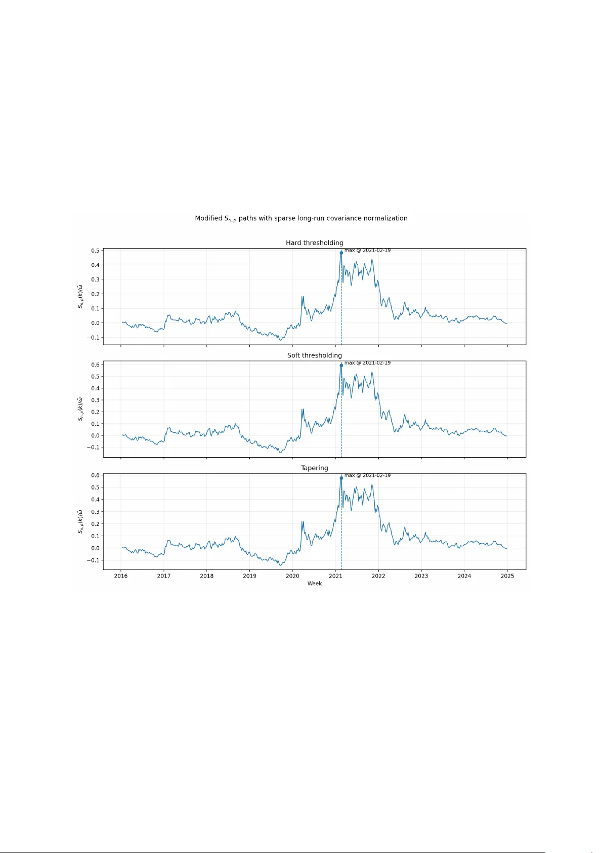
Diﬀerence-Based High-Dimensional Long-Run Co v ariance Matrix Estimation for Mean-shift Time Series Y anhong Liu 1 , F engyi Song 2 , and Long F eng 2 1 Guangzhou Universit y , 2 Nank ai Universit y Marc h 19, 2026 Abstract W e consider estimation of high-dimensional long-run co v ariance matrices for time series with nonconstant means, a setting in which con ven tional estimators can be severely biased. T o address this diﬃculty , we propose a diﬀerence-based initial estimator that is robust to a broad class of mean v ariations, and com bine it with hard thresholding, soft thresholding, and tap ering to obtain sparse long-run cov ariance estimators for high-dimensional data. W e deriv e con vergence rates for the resulting estimators under general temp oral dep endence and time-v arying mean structures, showing explicitly ho w the rates dep end on cov ariance sparsit y , mean v ariation, dimension, and sample size. Numerical exp eriments sho w that the prop osed methods perform fav orably in high dimensions, esp ecially when the mean evolv es o v er time. Keyw ords: diﬀerence-based estimator; long-run co v ariance matrix; high dimension; thresholding; max-norm con vergence; nonstationary mean. 1 In tro duction Let { X t } n t =1 b e a p -dimensional time series. A fundamen tal second-order ob ject in time series analysis is the long-run co v ariance matrix V := ∞ X k = −∞ Γ k , Γ k := Co v ( Z 0 , Z k ) , where { Z t } denotes the latent stationary noise c omponent. When the sp ectral density ma- trix f Z ( ω ) exists, V = 2 π f Z (0), so V is precisely the zero-frequency summary of temp oral dep endence. This matrix plays a central role in statistical inference for temp orally dep enden t data, including inference for sample means and linear con trasts, change-point analysis, trend inference, sim ultaneous conﬁdence bands, and many other procedures driven b y partial sums or temp orally aggregated quantities ( Newey and W est , 1987 ; Andrews , 1991 ; Chan , 2022a , b ). In lo w-dimensional settings, long-run v ariance or long-run co v ariance estimation has b een exten- siv ely studied through heteroskedasticit y and auto correlation consisten t (HA C) estimators and related k ernel or bandwidth-based pro cedures ( New ey and W est , 1987 ; Andrews , 1991 ). Classical HA C metho dology is typically developed under the implicit premise that the observ ed series can b e globally centered without materially distorting the serial dep endence structure. This paradigm is adequate when the mean is stable, but it can break down when the data contain smo oth trends, abrupt level shifts, or multiple c hange p oin ts. In such settings, naiv e 1 cen tering ma y contaminate sample auto co v ariances, thereby leading to seriously biased long-run v ariance estimates. T o ov ercome this diﬃcult y , Chan ( 2022a ) and Chan ( 2022b ) developed mean- structure-robust, diﬀerence-based estimators that remain v alid under unkno wn trends and ev en a possibly divergen t n umber of breaks. How ev er, that literature is essentially low-dimensional and does not address the additional regularization required when the am bient dimension p is comparable to or m uch larger than the sample size n . Mean while, the high-dimensional cov ariance literature has largely evolv ed from the i.i.d. setting. It is now well understo od that the sample co v ariance matrix is no longer a reliable estimator when p is large relativ e to n , which has led to a rich b ody of work on regularized co v ariance estimation. Representativ e examples include hard thresholding ( Bick el and Levina , 2008 ), generalized thresholding and shrink age ( Rothman et al. , 2009 ), adaptiv e thresholding ( Cai and Liu , 2011 ), and tapering-based estimators ( Cai et al. , 2010 ). These metho ds exploit sparsit y or approximate sparsit y of the target cov ariance matrix and ha ve b ecome standard to ols in mo dern high-dimensional inference. How ev er, they are designed primarily for con temp oraneous co v ariance matrices under indep endence, and therefore do not directly address the cumulativ e serial dep endence encoded in V . A growing literature extends high-dimensional second-order estimation to temp orally de- p enden t observ ations, but the main target in that line of w ork is still the contemporaneous co v ariance matrix Σ = Co v ( Z t ) or its inv erse, rather than the long-run cov ariance matrix V . F or example, Chen et al. ( 2013 ) established rates for thresholded cov ariance and graphical-Lasso-type precision matrix estimation for high-dimensional stationary and locally stationary time series under functional dep endence conditions. Sh u and Nan ( 2019 ) further developed generalized thresholding and precision matrix estimation for temp orally dep endent observ ations, allo wing slo wly decaying dep endence and long memory through auto correlation-based dep endence sum- maries. Under hea vy tails and mild momen ts, Zhang ( 2021 ) studied robust estimation of means, co v ariance matrices and precision matrices for high-dimensional time series. Although these pap ers substan tially broaden the scope of high-dimensional co v ariance analysis under dep endence, their inferen tial target remains Σ or Σ − 1 rather than the long-run cov ariance matrix needed for inference on temporal aggregates. Related frequency-domain w ork considers high-dimensional sp ectral density matrices and their inv erses. Sun et al. ( 2018 ) proposed thresholded estimators for large sp ectral density matrices of Gaussian and linear pro cesses. Fiecas et al. ( 2019 ) developed non-asymptotic theory for smo othed p eriodogram estimation and sparse in verse spectral densit y estimation. F or lo cally stationary pro cesses, Zhang and W u ( 2021 ) deriv ed a systematic asymptotic theory for co v ariance and sp ectral density estimation in high dimensions. These papers are highly relev ant b ecause the sp ectral density matrix is the frequency-domain analogue of the cov ariance structure. Nev ertheless, they do not directly solve the problem considered here, namely , estimating a sparse long-run co v ariance matrix in the time domain when the observ ed series ma y con tain nonconstan t and unknown mean structures. There is also a more recen t line of work that comes closer to the present problem by directly targeting zero-frequency or long-memory ob jects. In particular, Baek et al. ( 2023 ) dev elop ed thresholded and p enalized lo cal Whittle estimators for high-dimensional long-run v ariance and precision matrices under short- and long-range dep endence, and Zhang et al. ( 2025 ) studied joint estimation of multiple precision matrices for long-memory time series. These contributions demonstrate that high-dimensional long-run second-order estimation is b oth statistically meaningful and technically challenging. Ho wev er, the existing metho ds in this direction are mainly form ulated in the frequency domain under stationary models, whereas man y applications in econometrics, ﬁnance, environmen tal studies, and neuroscience in volv e unkno wn trends, structural breaks, or other nonstationary mean dynamics. This creates a gen uine metho dological gap b etw een mean-robust long-run v ariance estimation in classical time 2 series and sparse regularization in mo dern high-dimensional statistics. The goal of this paper is to ﬁll this gap. W e study diﬀer enc e-b ase d high-dimensional long-run c ovarianc e matrix estimation for multiv ariate time series. Our starting p oin t is a diﬀerence-based pilot estimator motiv ated by Chan ( 2022b ), whic h is intrinsically robust to a broad class of mean structures. W e then com bine this pilot estimator with three regularization sc hemes that are standard in high-dimensional cov ariance estimation, namely , hard thresholding, soft thresholding, and tap ering. In this wa y , we bridge tw o strands of literature that ha ve largely dev elop ed separately: on the one hand, mean-structure-robust long-run v ariance estimation for dep endent data; on the other hand, sparse matrix regularization for high-dimensional co v ariance estimation. The prop osed framew ork has sev eral attractiv e features. First, b y using diﬀerence statistics instead of global centering, it remains stable when the observed series con tains smooth mean v ariation or abrupt mean changes. Second, the subsequen t regularization step exploits sparsity of the long-run cov ariance matrix and therefore adapts naturally to high-dimensional regimes. Third, our methodology is en tirely time-domain, making it conceptually simple and computationally con venien t, while still targeting the quantit y that is directly relev ant for inference based on partial sums and sample a verages. F rom a theoretical p ersp ectiv e, w e establish conv ergence prop erties for the hard-thresholded, soft-thresholded, and tap ered estimators under suitable dep endence and sparsit y conditions. F rom a numerical p ersp ective, our simulation results sho w that these procedures p erform well in genuinely high-dimensional settings and remain eﬀective when the mean structure is nonconstant, where classical HA C-t yp e estimators can deteriorate substan tially . The rest of the paper is organized as follo ws. Section 2 introduces the diﬀerence-based oracle and feasible long-run cov ariance estimators and the three regularization schemes. W e also establishes the main concentration and con vergence results. Section 3 rep orts simulation studies under b oth constan t and nonconstant mean structures. In Section 4 , w e apply our metho d to a c hange-p oint inference problem for time series. Section 5 concludes the pap er. 2 Metho ds 2.1 Diﬀerence-based long-run co v ariance matrix estimation Let X t = µ t + Z t , t = 1 , . . . , n, where X t , µ t , Z t ∈ R p n , p n is allow ed to diverge with n , and { Z t } t ∈ Z is a zero-mean strictly stationary pro cess. Deﬁne the lag- k auto cov ariance matrix of Z t b y Γ k := E  Z 0 Z ⊤ k  , k ∈ Z . The target long-run co v ariance matrix is V := X k ∈ Z Γ k ∈ R p n × p n , assuming the series con verges entrywise (equiv alently , in max norm under our assumptions). Supp ose that µ 1 = · · · = µ n . A large b o dy of work has b een devoted to estimating the long-run cov ariance matrix V , and the existing metho ds may b e broadly group ed into three classical categories. The ﬁrst category consists of subsampling-based estimators; see, for example, Mek eton and Sc hmeiser ( 1984 ); Carlstein ( 1986 ); Song and Schmeiser ( 1995 ); P olitis et al. ( 1999 ); Chan and Y au ( 2017 ). A represen tative example is the o verlapping batch means (OBM) 3 estimator, b Σ OBM ,n := ℓ n − ℓ + 1 n X i = ℓ   1 ℓ i X j = i − ℓ +1 c X j   ⊗ 2 , where ℓ ∈ N ∩ (1 , n ) is the batc h size, c X i = X i − X n , and X n = n − 1 P n i =1 X i . And a ⊗ 2 := a ⊗ a = aa ⊤ for an y a ∈ R p . The second category is formed by kernel-based estimators; see Newey and W est ( 1987 ); Andrews ( 1991 ); Politis ( 2011 ). Two widely used examples are the Bartlett and quadratic sp ectral (QS) estimators, b Σ Bart ,n := ℓ X k = − ℓ Bart( k /ℓ ) b Γ k , b Σ QS ,n := n − 1 X k = − ( n − 1) QS( k /ℓ ) b Γ k , where b Γ k := n − 1 n X i = | k | +1 c X i c X ⊤ i −| k | , Bart( t ) := (1 − | t | ) I ( | t | ≤ 1) , and QS( t ) := 25 12 π 2 t 2  sin(6 π t/ 5) 6 π t/ 5 − cos(6 π t/ 5)  . The third category includes resampling-based pro cedures; see, for instance, K ¨ unsc h ( 1989 ); P olitis and Romano ( 1994 ); P aparo ditis and Politis ( 2001 ); Lahiri ( 2003 ). More recen tly , another line of research has dev elop ed estimators constructed from orthonormal series; see Phillips ( 2005 ); Sun ( 2013 ). Practical issues concerning the choice of kernels and orthonormal bases are discussed in Lazarus et al. ( 2018 ), while M ¨ uller ( 2014 ) inv estigated inference in the presence of strong serial dep endence. When the mean structure is nonconstant, that is, µ i  = µ j for some i  = j , the classical estimators of the long-run co v ariance matrix may fail to b e v alid. In particular, standard HA C-type estimators are generally biased unless the mean is constant, and existing mo diﬁcations for nonstationary time series are typically tailored to sp eciﬁc forms of mean structure and are not equipp ed with an implemen table optimal bandwidth selector. T o address this diﬃculty , Chan ( 2022a ) prop osed a mean-structure and auto correlation consistent (MA C) estimator, which is fully nonparametric and can b e computed in a single pass without explicitly estimating the trend or locating change p oin ts. The k ey idea is to use a v ariate-diﬀerence and bi-diﬀerencing construction to remo ve the eﬀect of the unknown mean structure. Sp eciﬁcally , deﬁne b ∆ k = 1 2( n − | k | + 1) n X i = | k | +1  X i − X i −| k |  ⊗ 2 , | k | = 0 , 1 , . . . , n − 1 . Let L k = c 0 ℓ + c 1 | k | with c 0 , c 1 > 0. Then the MA C estimator of V is given b y b V 0 ,q ,n = ℓ X k = − ℓ K q  | k | ℓ   b ∆ L k − b ∆ k  , K q ( x ) = (1 − | x | q ) 1 ( | x | ≤ 1) , whic h yields an estimator that is robust to unkno wn trends and m ultiple change points. Chan ( 2022b ) prop osed a general framework for the estimation of the long-run v ariance for time series with nonconstant means. W e adopt the diﬀerence-based construction in the 4 m ultiv ariate extension of Chan ( 2022b ). Let m n ∈ N b e the diﬀerence order and h n ∈ N the lag spacing. Let d n = ( d n, 0 , . . . , d n,m n ) ⊤ b e a normalized diﬀerence sequence satisfying m n X j =0 d n,j = 0 , m n X j =0 d 2 n,j = 1 . (1) Deﬁne the v ector-v alued diﬀerence statistics D t := m n X j =0 d n,j X t − j h n , t = m n h n + 1 , . . . , n. F or each integer k with | k | < ℓ n , where ℓ n is the kernel bandwidth, deﬁne the diﬀerence-based sample auto co v ariance matrix b Γ D k := 1 n n X t = m n h n + | k | +1 D t D ⊤ t −| k | . Let K ( · ) b e an even kernel supp orted on [ − 1 , 1]. The initial diﬀerence-based long-run co v ariance matrix estimator is b V DB := X | k | <ℓ n K  k ℓ n  b Γ D k . T o retain the mean con tribution explicitly , deﬁne M t := m n X j =0 d n,j µ t − j h n , U t := m n X j =0 d n,j Z t − j h n , (2) so that D t = M t + U t . Deﬁne the oracle auto co v ariance estimator (built from the noise-only diﬀerence pro cess) b y b Γ U k := 1 n n X t = m n h n + | k | +1 U t U ⊤ t −| k | , b V or := X | k | <ℓ n K  k ℓ n  b Γ U k . The mean-only deterministic con tribution is B µ,n := X | k | <ℓ n K  k ℓ n    1 n n X t = m n h n + | k | +1 M t M ⊤ t −| k |   . (3) Deﬁne the residual mean-induced random remainder R µ,n := b V DB − b V or − B µ,n . (4) By construction, R µ,n consists of the cross terms inv olving M t and U t . W e do not imp ose a c hangep oint structure on µ t ; instead, B µ,n and R µ,n will en ter the conv ergence rate explicitly . W e now state assumptions needed for the high-dimensional max-norm analysis. These assumptions are designed to (i) preserv e the construction of the estimator detailed in Section 6.2 of Chan ( 2022b ), (ii) k eep the mean-induced eﬀect explicit, and (iii) enable a high-dimensional union-b ound upgrade of the entrywise oracle concentration. Assumption 2.1 (Kernel and diﬀerence sequence) . The kernel K is even, b ounde d, supp orte d on [ − 1 , 1] , and K (0) = 1 . Ther e exist c onstants q 0 > 0 and C K > 0 such that | 1 − K ( x ) | ≤ C K | x | q 0 , | x | ≤ 1 . The diﬀer enc e se quenc e { d n,j } m n j =0 is normalize d as in e quation ( 1 ) . Mor e over, m n h n = o ( n ) , ℓ n → ∞ , ℓ n = o ( n ) . 5 Assumption 2.2 (Uniform oracle bias bound inherited from DB k ernel theory) . Ther e exists a c onstant C B > 0 , indep endent of n and ( r, s ) , such that    E ( b V or ) − V    max ≤ C B  ℓ − q 0 n + ( m n + 1) h n n  . Assumption 2.3 (Uniform Bernstein-t yp e concentration for oracle entries) . Ther e exist c onstants c 1 , c 2 > 0 such that for al l suﬃciently lar ge n , al l 1 ≤ r , s ≤ p n , and al l t > 0 , P     b V or [ r , s ] − E b V or [ r , s ]    > t  ≤ 2 exp  − c 1 n min  t 2 ℓ n + m n h n , t ℓ n + m n h n  . R emark 2.1 . Assumptions 2.2 and 2.3 are standard in high-dimensional analysis of dep enden t data. They typically follow under suitable com binations of w eak temp oral dependence, such as ph ysical dep endence or mixing conditions, together with mild tail assumptions, for example, sub- exp onen tial or Bernstein-type momen t b ounds on the co ordinates. W e state these assumptions directly in the main text b ecause the primary goal of this pap er is to develop the max-norm error analysis and the asso ciated thresholding theory for the diﬀerence-based estimator in a high-dimensional setting. F or completeness, the app endix pro vides several suﬃcient conditions under whic h b oth assumptions are satisﬁed. Assumption 2.4 (Explicit mean-induced remainder) . Ther e exists a deterministic se quenc e r µ,n ≥ 0 such that ∥ R µ,n ∥ max = O p ( r µ,n ) , wher e R µ,n is deﬁne d in e quation ( 4 ) . R emark 2.2 . Assumption 2.4 do es not require µ t to follo w a changepoint mo del. The mean eﬀect is fully retained through the explicit deterministic bias matrix B µ,n in equation ( 3 ) and the remainder R µ,n . A detailed discussion of mean shifts is pro vided in Section 2.4 . Next, w e state the Max-norm rate of the initial diﬀerence-based estimator b V DB . Deﬁne the o verall rate a n := ∥ B µ,n ∥ max + r µ,n + ℓ − q 0 n + ( m n + 1) h n n + r ( ℓ n + m n h n ) log p n n + ( ℓ n + m n h n ) log p n n . (5) Theorem 2.1. Supp ose Assumptions 2.1 – 2.4 hold and log p n = o ( n ) . Then    b V DB − V    max = O p ( a n ) , wher e a n is deﬁne d in ( 5 ) . Corollary 2.1 (Bandwidth-balanced rate under negligible mean remainder) . Assume the c onditions of The or em 2.1 . In addition, supp ose ∥ B µ,n ∥ max + r µ,n = o ℓ − q 0 n + r ℓ n log p n n ! , m n h n ≲ ℓ n , ( m n + 1) h n n = o ℓ − q 0 n + r ℓ n log p n n ! . Then    b V DB − V    max = O p ℓ − q 0 n + r ℓ n log p n n + ℓ n log p n n ! . If mor e over ℓ n log p n /n → 0 and ℓ n ≍  n log p n  1 / (2 q 0 +1) , then    b V DB − V    max = O p (  log p n n  q 0 / (2 q 0 +1) ) . (6) 6 2.2 Sparse Estimators When the dimension is ﬁxed, the diﬀerence-based (DB) estimator is eﬀectiv e for time series with nonconstan t mean structures. In high-dimensional settings, ho wev er, the DB estimator may suﬀer from substantial bias and may fail to b e in v ertible, muc h like the sample cov ariance matrix in classical high-dimensional problems. This motiv ates the use of sparse regularization under the assumption that the long-run cov ariance matrix is sparse. In this pap er, we fo cus on three widely used regularization schemes: hard thresholding ( Bic kel and Levina , 2008 ), soft thresholding ( Rothman et al. , 2009 ), and tapering ( Cai et al. , 2010 ). W e note that other high-dimensional co v ariance estimators developed in the literature could also be com bined with the DB estimator in a similar manner. Let τ n > 0 b e a threshold lev el. Deﬁne the hard-thresholding estimator b V hard = ( b V hard rs ) b y b V hard rs =    b V DB [ r , r ] , r = s, b V DB [ r , s ] 1  | b V DB [ r , s ] | ≥ τ n  , r  = s. (7) Similarly , deﬁne the soft-thresholding estimator b V soft = ( b V soft rs ) b y b V soft rs =    b V DB [ r , r ] , r = s, sign( b V DB [ r , s ])  | b V DB [ r , s ] | − τ n  + , r  = s. (8) Assumption 2.5 (W eak ro w-sparsity class) . Ther e exist α ∈ [0 , 1) , M > 0 , and a se quenc e c n,p ≥ 1 such that V is symmetric and max 1 ≤ r ≤ p n p n X s =1 | V rs | α ≤ c n,p , max 1 ≤ r ≤ p n V rr ≤ M . Theorem 2.2 (Thresholded estimation under w eak row-sparsit y) . Supp ose The or em 2.1 and Assumption 2.5 hold. L et τ n = C τ a n with a suﬃciently lar ge c onstant C τ > 0 . Then, for the har d-thr esholding estimator b V hard ,    b V hard − V    max = O p ( a n ) , (9)    b V hard − V    2 = O p  c n,p a 1 − α n  , (10) 1 p n    b V hard − V    2 F = O p  c n,p a 2 − α n  . (11) In p articular, if c n,p a 1 − α n → 0 , then b V hard is op er ator-norm c onsistent. Theorem 2.3 (Soft-thresholding under weak ro w-sparsity) . Supp ose The or em 2.1 and Assump- tion 2.5 hold. L et τ n = C τ a n with C τ > 0 suﬃciently lar ge, then, for the soft-thr esholding estimator b V soft ,    b V soft − V    max = O p ( a n ) , (12)    b V soft − V    2 = O p  c n,p a 1 − α n  , (13) 1 p n    b V soft − V    2 F = O p  c n,p a 2 − α n  . (14) Theorems 2.2 and 2.3 establish the rates of con vergence for the hard-thresholding and soft- thresholding estimators, respectively . These rates dep end on sev eral key features of the problem, 7 most notably the sparsity lev el of the long-run cov ariance matrix, the magnitude of the mean shift, and the relationship b et ween the sample size and the dimension. Roughly sp eaking, a sparser co v ariance structure facilitates more accurate estimation, while a larger mean shift deteriorates performance through its impact on the bias term. Mean while, the dimensionalit y aﬀects the sto chastic error through the usual high-dimensional scaling. Consequen tly , the o verall conv ergence b ehavior is gov erned by the interpla y among dep endence sparsity , signal con tamination from the mean shift, and the eﬀective amoun t of sample information. These results clarify the regimes under whic h thresholded estimators remain reliable for estimating the long-run co v ariance matrix in high-dimensional settings. Deﬁnition 2.1 (T ap ering w eights and tapering estimator) . F or an integer k n ≥ 1, let W ( k n ) = ( w ( k n ) rs ) 1 ≤ r,s ≤ p n b e a symmetric tap ering weigh t matrix satisfying: (i) 0 ≤ w ( k n ) rs ≤ 1 for all r, s ; (ii) w ( k n ) rs = 1 if | r − s | ≤ k n / 2; (iii) w ( k n ) rs = 0 if | r − s | ≥ k n ; (iv) for eac h row r , the n umber of nonzero weigh ts # { s : w ( k n ) rs  = 0 } ≤ C w k n , where C w is a univ ersal constant. Deﬁne the tapering estimator by the Hadamard pro duct V tap := W ( k n ) ◦ b V DB . (15) T o establish the conv ergence rate of the tap ering estimator, we need the following assumption. Assumption 2.6 (Bandable target class) . Ther e exist ν > 0 , c onstants C bd , C bd , 2 , M 1 > 0 , such that V is symmetric and: max 1 ≤ r ≤ p n p n X s =1 | V rs | ≤ M 1 , max 1 ≤ r ≤ p n X | r − s | >k | V rs | ≤ C bd k − ν , ∀ k ≥ 1 , 1 p n p n X r =1 X | r − s | >k V 2 rs ≤ C bd , 2 k − 2 ν , ∀ k ≥ 1 . (16) Theorem 2.4 (T ap ering under bandability) . Supp ose The or em 2.1 , Assumption 2.6 , and Deﬁnition 2.1 hold. Then   V tap − V   2 = O p  k n a n + k − ν n  . (17) In addition, 1 p n   V tap − V   2 F = O p  k n a 2 n + k − 2 ν n  . (18) Henc e, if k n a n → 0 and k n → ∞ , the tap ering estimator is op er ator-norm c onsistent. The b alancing choic e k n ≍ a − 1 / ( ν +1) n yields   V tap − V   2 = O p  a ν / ( ν +1) n  . Theorem 2.4 is complemen tary to thresholding: thresholding targets sparse matrices without an index-distance structure, whereas tap ering exploits a natural ordering and bandability . Both are driv en by the same initial max-norm rate a n , whic h in our framework explicitly carries the mean-induced comp onen t. 8 2.3 Selection of tuning parameters The regularization parameters are selected in a data-driven manner through a blo ckwise v ali- dation pro cedure tailored to dep endent observ ations. Since random splitting at the individual- observ ation level w ould destroy the temp oral dep endence structure, w e instead rep eatedly draw t wo non-o verlapping contiguous blo c ks from the sample. F or the b th repetition, denote b y I tr b and I v a b the training blo c k and the v alidation blo ck, resp ectiv ely , and let ˆ V ( b ) λ b e the thresholded estimator of the diﬀerence-based long-run co v ariance matrix constructed from the training blo ck with threshold level λ . T o ev aluate the qualit y of ˆ V ( b ) λ , w e compute on the v alidation blo c k a pilot estimator ˜ V ( b ) , and measure the discrepancy by the squared F rob enius loss L b ( λ ) =   ˆ V ( b ) λ − ˜ V ( b )   2 F . Av eraging ov er B random double-blo ck splits yields the v alidation criterion CV λ ( λ ) = 1 B B X b =1 L b ( λ ) , and the selected threshold parameter is deﬁned by ˆ λ = arg min λ ∈ Λ CV λ ( λ ) , where Λ is a presp eciﬁed candidate set. This criterion formalizes the usual bias–v ariance trade-oﬀ: an excessively small λ retains to o man y spurious small entries and leads to high v ariability , whereas an excessiv ely large λ o vershrinks the co v ariance structure and induces substantial bias. The tap ering bandwidth k taper is c hosen according to the same principle. F or each candidate k ∈ K , let ˆ V ( b ) k denote the tap ering estimator computed from the training blo c k with bandwidth k . Its v alidation loss is deﬁned as L b ( k ) =   ˆ V ( b ) k − ˜ V ( b )   2 F , and the corresponding av erage criterion is CV k ( k ) = 1 B B X b =1 L b ( k ) . W e then select ˆ k taper = arg min k ∈K CV k ( k ) . F rom a statistical p ersp ectiv e, k taper con trols the eﬀective range of serial dep endence retained in the estimator: a small bandwidth may remo ve non-negligible auto cov ariance con tributions and th us incur truncation bias, while a large bandwidth tends to preserve more long-lag information at the cost of increased estimation v ariabilit y . Therefore, the prop osed blo c kwise v alidation rule pro vides a practically stable and theoretically reasonable calibration mec hanism for b oth λ and k taper , while respecting the dep endence structure of the time series. 2.4 Discussion of Means The rate a n in equation ( 5 ) con tains tw o mean-related components, ∥ B µ,n ∥ max and r µ,n , 9 where B µ,n is the deterministic mean-induced bias matrix in ( 3 ) and r µ,n con trols the sto chastic cross-term remainder R µ,n in ( 4 ) . W e now provide concrete upp er bounds under broad mean regularit y classes. Recall M t from ( 2 ). Deﬁne ¯ M 2 ,n := 1 n n X t = m n h n +1 ∥ M t ∥ 2 max , ¯ M ∞ ,n := max m n h n +1 ≤ t ≤ n ∥ M t ∥ max . (19) Also write ∥ K ∥ ∞ := sup | x |≤ 1 | K ( x ) | and L n := ℓ n + m n h n for short. Prop osition 2.1 (Generic deterministic b ound for B µ,n ) . Under Assumption 2.1 , the determin- istic me an-induc e d bias matrix B µ,n in ( 3 ) satisﬁes ∥ B µ,n ∥ max ≤ (2 ℓ n − 1) ∥ K ∥ ∞ ¯ M 2 ,n . Henc e ∥ B µ,n ∥ max = O ( ℓ n ¯ M 2 ,n ) . T o control the sto chastic mean-induced remainder R µ,n , w e imp ose a conditional Bernstein inequalit y on the cross terms. This assumption is standard once U t admits suitable dep endence and tail con trols uniformly ov er co ordinates, and M t is treated as deterministic conditioning information. Assumption 2.7 (Conditional Bernstein inequality for the mean-noise cross term) . Ther e exists a c onstant c 3 > 0 such that, c onditional on { µ t } n t =1 , for al l suﬃciently lar ge n and al l t > 0 , P  ∥ R µ,n ∥ max > t   { µ t } n t =1  ≤ 4 p 2 n exp  − c 3 n min  t 2 L 2 n ¯ M 2 ,n , t L n ¯ M ∞ ,n  . W e also give a suﬃcient condition for Assumption 2.7 in the App endix. Prop osition 2.2 (Generic stochastic b ound for R µ,n ) . Supp ose Assumption 2.7 holds and log p n = o ( n ) . Then ∥ R µ,n ∥ max = O p q ¯ M 2 ,n L n r log p n n + ¯ M ∞ ,n L n log p n n ! . (20) Conse quently, one may take r µ,n ≍ q ¯ M 2 ,n L n r log p n n + ¯ M ∞ ,n L n log p n n . (21) W e next show how ¯ M 2 ,n and ¯ M ∞ ,n can b e bounded under t w o concrete mean classes. 2.4.1 Piecewise-H¨ older mean class (with p ossible jumps) Assumption 2.8 (Piecewise-H¨ older mean path) . Ther e exist an inte ger J n ≥ 0 , a p artition 0 = η 0 < η 1 < · · · < η J n < η J n +1 = 1 , a H¨ older exp onent β ∈ (0 , 1] , and c onstants L µ , M µ > 0 such that for e ach c o or dinate r ∈ { 1 , . . . , p n } , µ ( r ) t = g r ( t/n ) , t = 1 , . . . , n, 10 wher e g r may jump at η 1 , . . . , η J n , satisﬁes sup u ∈ [0 , 1] | g r ( u ) | ≤ M µ , and on e ach op en interval ( η j , η j +1 ) , | g r ( u ) − g r ( v ) | ≤ L µ | u − v | β , ∀ u, v ∈ ( η j , η j +1 ) . Prop osition 2.3 (Mean-bias and remainder under piecewise-H¨ older means) . Supp ose Assump- tion 2.8 holds. L et C d, 1 := m n X j =0 | d n,j | , C d,β := m n X j =1 | d n,j | j β . Then: (i) The diﬀer enc e-me an pr o c ess satisﬁes ¯ M 2 ,n ≤ C (  h n n  2 β C 2 d,β + C 2 d, 1 M 2 µ J n m n h n n ) , (22) and ¯ M ∞ ,n ≤ C ( C d,β  h n n  β + C d, 1 M µ ) . (23) (ii) Conse quently, by Pr op osition 2.1 , ∥ B µ,n ∥ max ≤ C ℓ n (  h n n  2 β C 2 d,β + C 2 d, 1 M 2 µ J n m n h n n ) . (24) (iii) If Assumption 2.7 also holds, then by Pr op osition 2.2 , ∥ R µ,n ∥ max = O p v u u t (  h n n  2 β C 2 d,β + C 2 d, 1 M 2 µ J n m n h n n ) L n r log p n n + ( C d,β  h n n  β + C d, 1 M µ ) L n log p n n ! . (25) Her e C > 0 is a c onstant indep endent of n and p n . 2.4.2 Bounded-v ariation mean class (no changepoint parametrization) Assumption 2.9 (Co ordinatewise discrete b ounded v ariation) . Ther e exists M µ > 0 and a se quenc e V µ,n ≥ 0 such that sup 1 ≤ t ≤ n ∥ µ t ∥ max ≤ M µ and max 1 ≤ r ≤ p n n X t =2    µ ( r ) t − µ ( r ) t − 1    ≤ V µ,n . 11 Prop osition 2.4 (Mean-bias and remainder under b ounded-v ariation means) . Supp ose Assump- tion 2.9 holds. L et C d, 1 := P m n j =0 | d n,j | . Then ¯ M 2 ,n ≤ C C 2 d, 1 ( m n h n ) 2 V 2 µ,n n , (26) and ¯ M ∞ ,n ≤ 2 C d, 1 M µ . (27) Conse quently, ∥ B µ,n ∥ max ≤ C ℓ n C 2 d, 1 ( m n h n ) 2 V 2 µ,n n , (28) and, if Assumption 2.7 holds, ∥ R µ,n ∥ max = O p  C d, 1 m n h n V µ,n L n √ log p n n + C d, 1 M µ L n log p n n  . (29) R emark 2.3 (Plug-in rates for a n ) . Theorem 2.1 remains unc hanged, but Prop ositions 2.3 and 2.4 pro vide explicit, directly usable upper b ounds for the mean-related comp onen ts in a n . F or example, under Assumption 2.8 , one may substitute ( 24 ) and ( 25 ) into ( 5 ). Corollary 2.2 (Explicit a n under piecewise-H¨ older means) . Supp ose the c onditions of The o- r em 2.1 hold, and Assumptions 2.7 and 2.8 hold. Then one may cho ose a n ≍ ℓ − q 0 n + ( m n + 1) h n n + r L n log p n n + L n log p n n + ℓ n (  h n n  2 β C 2 d,β + C 2 d, 1 M 2 µ J n m n h n n ) + v u u t (  h n n  2 β C 2 d,β + C 2 d, 1 M 2 µ J n m n h n n ) L n r log p n n + ( C d,β  h n n  β + C d, 1 M µ ) L n log p n n . In p articular, if the me an-induc e d terms ar e of smal ler or der than the or acle terms, the r ate r e duc es to the b andwidth-b alanc e d form in Cor ol lary 2.1 . 3 Sim ulation W e conduct Mon te Carlo experiments to assess ﬁnite-sample p erformance of high-dimensional long-run co v ariance (LR C) matrix estimation under temporal dep endence and cross-sectional dep endence. F or eac h replication, we generate a p -v ariate time series { X t } n t =1 with diﬀeren t sample sizes n = 200 , 400 , 800 , 1600 and dimensions p = 300 , 500. The temp oral dep endence follo ws an AR(1) recursion Z t = ϕ Z t − 1 + ε t , t = 2 , . . . , n, with ϕ = 0 . 5, and w e discard an initial burn-in of length 200 to mitigate initialization eﬀects. Throughout, the inno v ations { ε t } are i.i.d. Gaussian with mean zero and co v ariance matrix Σ ε , whose structure diﬀers across the following t wo mo dels. Mo del I (tridiagonal cross-sectional dep endence). W e imp ose lo cal cross-sectional dep endence b y taking Σ ε to b e tridiagonal. Speciﬁcally , let a = 0 . 5 and deﬁne Σ ε b y ( Σ ε ) 11 = 1 , ( Σ ε ) ii = 1 + a 2 ( i ≥ 2) , ( Σ ε ) i,i − 1 = ( Σ ε ) i − 1 ,i = a ( i ≥ 2) , and ( Σ ε ) ij = 0 otherwise. 12 Mo del I I (T o eplitz cross-sectional dependence). W e consider a bandable T o eplitz co v ariance with exp onen tial decay: ( Σ ε ) ij = ρ | i − j | , ρ = 0 . 7 , 1 ≤ i, j ≤ p. Mo del I I I (P ermuted Blo c k Diagonal Structure). W e generate data from a multiv ariate mo del with co v ariance matrix Σ = ΠΣ 0 Π ⊤ , Σ 0 = diag( B , . . . , B ) , B =  1 ρ ρ 1  , where Π is a permutation matrix. This co v ariance matrix is highly sparse, since eac h ro w has only one nonzero oﬀ-diagonal en try , but it is not banded after p erm utation. T o examine robustness to nonconstant means, we add a deterministic mean com ponent to the ﬁrst m = 20 co ordinates of the observ ed series. Let t = i/n for i = 1 , . . . , n and deﬁne µ ( t ) = exp( t ) + 1 ( t > 0 . 3) + 2 1 ( t > 0 . 6) + 4 1 ( t > 0 . 8) . W e set E ( X t,j ) = µ ( t ) for j = 1 , . . . , m and E ( X t,j ) = 0 for j > m . The target LR C matrix is deﬁned for the cen tered stationary comp onen t and, under b oth models, equals V = ∞ X k = −∞ Γ ( k ) = Σ ε (1 − ϕ ) 2 , where Γ ( k ) = Co v ( X t , X t − k ). W e compare six estimators of V . 1. HA C. The standard heterosk edasticity and autocorrelation consistent estimator of New ey and W est ( 1987 ). F or a fair comparison, we use the same k ernel as in the DB estimator, namely K q ( u ) = (1 − | u | q ) + , q = 2 . 2. MA C. The mean-structure and auto correlation consisten t co v ariance matrix estimator prop osed b y Chan ( 2022a ). 3. DB. The diﬀerence-based estimator proposed by Chan ( 2022b ). In our implementation, w e set m = 3 and use d = (0 . 1942 , 0 . 2809 , 0 . 3832 , − 0 . 8582) ⊤ . W e choose h n = 2 ℓ n and ℓ n = min   n log p  1 / 4  ,  n − 10 28   . 4. Hard. The hard-thresholded DB estimator deﬁned in ( 7 ). 5. Soft. The soft-thresholded DB estimator deﬁned in ( 8 ). 6. T ap er. The tap ered DB estimator deﬁned in ( 15 ) , where the tap ering weigh ts are giv en b y W ( k ) ij =      1 , | i − j | ≤ k / 2 , 2 − 2 | i − j | /k , k / 2 < | i − j | < k , 0 , | i − j | ≥ k . 13 F or each replication and eac h method, w e compute the estimation error E = b V − V and rep ort four matrix norms: ∥ E ∥ F , ∥ E ∥ 1 , ∥ E ∥ max , ∥ E ∥ 2 , where ∥ · ∥ F is the F rob enius norm, ∥ · ∥ 1 is the induced matrix 1-norm, ∥ · ∥ max = max i,j | E ij | is the en trywise maxim um norm, and ∥ · ∥ 2 is the spectral norm. W e also report their relativ e errors, obtained b y dividing each error norm b y the corresp onding norm of V (with a small n umerical safeguard in the denominator). Results are summarized as Monte Carlo a verages ov er 1000 replications. Sev eral conclusions emerge clearly from T ables 1 – 6 . First, the unregularized HAC estimator p erforms v ery p o orly in all six settings. Its absolute and relativ e errors remain extremely large across all matrix norms, and the impro vemen t with increasing sample size is negligible. This instabilit y is esp ecially pronounced under the induced ℓ 1 and sp ectral norms, indicating that direct high-dimensional HA C estimation is not reliable in the present regime. In the settings where the MA C estimator is rep orted, it improv es substan tially ov er HAC, but it is still uniformly less accurate than the diﬀerence-based pro cedures, particularly after s tructural regularization. By contrast, the raw DB estimator already ac hieves a dramatic reduction in error, and its accuracy impro ves steadily as n increases, conﬁrming the practical adv an tage of diﬀerencing for remo ving the nonstationary mean comp onen t b efore long-run co v ariance estimation. Second, the eﬀect of regularization dep ends in an informative wa y on the underlying cross- sectional structure. F or Mo dels I and I I, where the co v ariance matrix is banded or bandable under the observ ed ordering, the regularized DB estimators uniformly improv e up on the ra w DB estimator, and the tap ered estimator is typically the most accurate o verall. Its adv antage is especially clear under the F rob enius, matrix ℓ 1 , and sp ectral norms, and this pattern is stable for b oth p = 300 and p = 500. The gains from regularization are therefore not only substan tial but also robust to increasing dimensionality . In contrast, Model I II is sparse but explicitly non-banded after p ermutation. In this setting, the tap ering estimator loses m uch of its adv antage, while hard- and soft-thresholding b ecome more comp etitiv e and often outperform tap ering under the F rob enius norm, with soft-thresholding also p erforming very well under the sp ectral norm in sev eral cases. This contrast is consistent with the structural design of the three regularization schemes: tap ering is most eﬀective when the v ariable ordering carries meaningful lo cality information, whereas thresholding is better adapted to general sparsity without bandedness. Finally , across all six tables, the max-norm errors of the regularized estimators are often quite close to one another, suggesting that the main b eneﬁt of regularization lies in improving global matrix reco very rather than merely reducing the largest en trywise deviation. 4 Data Application F ollowing W ang et al. ( 2025 ), we study w eekly log-returns of NASDA Q constituen t sto c ks from Jan uary 2016 to December 2024. Financial return panels of this t yp e are w ell kno wn to exhibit substan tial temp oral dependence and strong cross-sectional como vemen t, so a realistic c hangep oint analysis must accoun t for the long-run co v ariance structure; see also the empirical discussion in W ang et al. ( 2025 ). Our ob jective is to examine whether the high-dimensional return pro cess experienced a structural break during the sample perio d. F ormally , let X 1 , . . . , X n ∈ R p denote the w eekly return v ectors where in our pro cessed sample n = 471 and p = 1556. W e consider the single-changepoint testing problem H 0 : µ 1 = · · · = µ n v ersus H 1 : µ 1 = · · · = µ τ  = µ τ +1 = · · · = µ n 14 T able 1: Estimation errors of diﬀerent metho ds under Mo del I with p = 300. Metho d ∥ E ∥ F ∥ E ∥ 1 ∥ E ∥ max ∥ E ∥ 2 ∥ E ∥ F ∥ V ∥ F ∥ E ∥ 1 ∥ V ∥ 1 ∥ E ∥ max ∥ V ∥ max ∥ E ∥ 2 ∥ V ∥ 2 ( n, p ) = (200 , 300) HA C 4106.84 6867.44 235.29 4088.23 41.31 763.05 47.06 454.26 MA C 298.80 395.14 7.05 113.76 3.01 43.90 1.41 12.64 DB 114.23 130.85 3.47 33.43 1.15 14.54 0.69 3.71 Hard 61.08 21.90 3.47 10.77 0.61 2.43 0.69 1.20 Soft 60.16 16.83 3.47 7.38 0.61 1.87 0.69 0.82 T ap er 47.54 6.44 3.47 5.56 0.48 0.72 0.69 0.62 ( n, p ) = (400 , 300) HA C 4269.37 6320.69 237.59 4258.68 42.95 702.30 47.52 473.20 MA C 233.92 280.08 4.94 74.85 2.35 31.12 0.99 8.32 DB 86.31 80.67 3.13 16.57 0.87 8.96 0.63 1.84 Hard 49.90 7.90 3.13 6.19 0.50 0.88 0.63 0.69 Soft 53.45 11.65 3.13 6.05 0.54 1.29 0.63 0.67 T ap er 45.44 5.83 3.13 5.07 0.46 0.65 0.63 0.56 ( n, p ) = (800 , 300) HA C 4350.53 5825.08 235.43 4344.89 43.76 647.23 47.09 482.78 MA C 179.73 199.80 3.62 49.01 1.81 22.20 0.72 5.45 DB 83.31 82.84 2.45 17.53 0.84 9.20 0.49 1.95 Hard 33.81 10.17 2.45 4.96 0.34 1.13 0.49 0.55 Soft 41.38 6.51 2.45 5.05 0.42 0.72 0.49 0.56 T ap er 30.99 4.56 2.45 3.87 0.31 0.51 0.49 0.43 ( n, p ) = (1600 , 300) HA C 4378.63 5425.14 232.24 4375.73 44.04 602.79 46.45 486.20 MA C 137.11 142.28 2.47 32.32 1.38 15.81 0.49 3.59 DB 72.96 71.94 1.89 15.02 0.73 7.99 0.38 1.67 Hard 27.09 11.41 1.89 5.21 0.27 1.27 0.38 0.58 Soft 30.45 8.61 1.89 4.01 0.31 0.96 0.38 0.45 T ap er 21.98 3.57 1.89 2.97 0.22 0.40 0.38 0.33 15 T able 2: Estimation errors of diﬀerent metho ds under Mo del II with p = 300. Metho d ∥ E ∥ F ∥ E ∥ 1 ∥ E ∥ max ∥ E ∥ 2 ∥ E ∥ F ∥ V ∥ F ∥ E ∥ 1 ∥ V ∥ 1 ∥ E ∥ max ∥ V ∥ max ∥ E ∥ 2 ∥ V ∥ 2 ( n, p ) = (200 , 300) HA C 4054.94 6474.14 226.25 4043.14 34.32 285.62 56.56 178.52 MA C 241.73 334.23 5.88 106.17 2.05 14.75 1.47 4.69 DB 100.44 108.19 2.78 28.82 0.85 4.77 0.69 1.27 Hard 75.79 26.32 2.83 17.90 0.64 1.16 0.71 0.79 Soft 78.71 27.24 2.78 17.91 0.67 1.20 0.70 0.79 T ap er 59.71 17.73 2.78 14.31 0.51 0.78 0.69 0.63 ( n, p ) = (400 , 300) HA C 4248.96 6027.40 230.56 4242.28 35.96 265.91 57.64 187.31 MA C 189.48 237.01 4.07 72.58 1.60 10.46 1.02 3.20 DB 79.35 67.94 2.51 17.12 0.67 3.00 0.63 0.76 Hard 64.03 18.88 2.51 15.40 0.54 0.83 0.63 0.68 Soft 69.15 22.26 2.51 16.01 0.59 0.98 0.63 0.71 T ap er 55.53 15.97 2.51 12.93 0.47 0.70 0.63 0.57 ( n, p ) = (800 , 300) HA C 4341.36 5634.79 230.95 4337.80 36.74 248.59 57.74 191.53 MA C 146.19 170.41 2.90 48.77 1.24 7.52 0.73 2.15 DB 71.74 69.05 1.95 16.10 0.61 3.05 0.49 0.71 Hard 46.80 16.35 1.96 11.97 0.40 0.72 0.49 0.53 Soft 56.43 17.77 1.97 14.03 0.48 0.78 0.49 0.62 T ap er 39.26 13.12 1.95 10.04 0.33 0.58 0.49 0.44 ( n, p ) = (1600 , 300) HA C 4372.59 5291.68 229.19 4370.74 37.00 233.46 57.30 192.99 MA C 112.72 123.15 2.01 33.86 0.95 5.43 0.50 1.50 DB 61.33 60.52 1.51 14.43 0.52 2.67 0.38 0.64 Hard 35.56 15.01 1.51 9.27 0.30 0.66 0.38 0.41 Soft 42.28 17.35 1.52 11.02 0.36 0.77 0.38 0.49 T ap er 28.73 10.70 1.51 7.69 0.24 0.47 0.38 0.34 16 T able 3: Estimation errors of diﬀerent metho ds under Mo del II I with p = 300. Metho d ∥ E ∥ F ∥ E ∥ 1 ∥ E ∥ max ∥ E ∥ 2 ∥ E ∥ F ∥ V ∥ F ∥ E ∥ 1 ∥ V ∥ 1 ∥ E ∥ max ∥ V ∥ max ∥ E ∥ 2 ∥ V ∥ 2 ( n, p ) = (200 , 300) HA C 4073.82 6571.00 233.42 4061.75 52.59 1095.17 58.35 676.96 DB 92.37 111.94 2.78 30.07 1.19 18.66 0.70 5.01 Hard 46.23 26.73 2.78 14.74 0.60 4.45 0.70 2.46 Soft 45.46 16.64 2.78 7.44 0.59 2.77 0.70 1.24 T ap er 47.57 4.78 2.78 4.57 0.61 0.80 0.70 0.76 ( n, p ) = (400 , 300) HA C 4253.51 6094.31 235.23 4246.63 54.91 1015.72 58.81 707.77 DB 69.03 67.77 2.52 14.60 0.89 11.30 0.63 2.43 Hard 36.64 8.79 2.52 4.41 0.47 1.47 0.63 0.73 Soft 40.29 10.47 2.52 4.28 0.52 1.75 0.63 0.71 T ap er 46.80 4.52 2.52 4.34 0.60 0.75 0.63 0.72 ( n, p ) = (800 , 300) HA C 4338.73 5657.96 232.83 4335.09 56.01 942.99 58.21 722.52 DB 67.04 69.93 1.96 15.66 0.87 11.65 0.49 2.61 Hard 27.07 12.86 1.96 6.23 0.35 2.14 0.49 1.04 Soft 30.29 5.59 1.96 3.50 0.39 0.93 0.49 0.58 T ap er 40.61 3.96 2.02 3.78 0.52 0.66 0.50 0.63 ( n, p ) = (1600 , 300) HA C 4374.31 5317.32 231.56 4372.45 56.47 886.22 57.89 728.74 DB 58.78 61.05 1.52 13.48 0.76 10.17 0.38 2.25 Hard 22.23 12.88 1.52 6.67 0.29 2.15 0.38 1.11 Soft 22.29 8.30 1.52 3.61 0.29 1.38 0.38 0.60 T ap er 37.78 3.84 2.00 3.42 0.49 0.64 0.50 0.57 17 T able 4: Estimation errors of diﬀerent metho ds under Mo del I with p = 500. Metho d ∥ E ∥ F ∥ E ∥ 1 ∥ E ∥ max ∥ E ∥ 2 ∥ E ∥ F ∥ V ∥ F ∥ E ∥ 1 ∥ V ∥ 1 ∥ E ∥ max ∥ V ∥ max ∥ E ∥ 2 ∥ V ∥ 2 ( n, p ) = (200 , 500) HA C 4257.80 8742.62 235.88 4207.16 33.16 971.40 47.18 467.47 MA C 489.54 627.42 6.85 163.23 3.81 69.71 1.37 18.14 DB 181.36 204.51 3.53 47.34 1.41 22.72 0.71 5.26 Hard 79.14 21.24 3.53 10.08 0.62 2.36 0.71 1.12 Soft 78.73 21.49 3.53 7.82 0.61 2.39 0.71 0.87 T ap er 61.79 6.61 3.53 5.66 0.48 0.73 0.71 0.63 ( n, p ) = (400 , 500) HA C 4345.56 7651.68 238.36 4316.10 33.85 850.19 47.67 479.57 MA C 386.65 452.15 5.16 107.04 3.01 50.24 1.03 11.89 DB 135.03 130.78 3.17 24.70 1.05 14.53 0.63 2.74 Hard 65.93 7.82 3.17 6.34 0.51 0.87 0.63 0.70 Soft 70.54 14.23 3.17 6.22 0.55 1.58 0.63 0.69 T ap er 59.38 6.36 3.17 5.16 0.46 0.71 0.63 0.57 ( n, p ) = (800 , 500) HA C 4394.94 6790.50 237.17 4379.21 34.23 754.50 47.43 486.58 MA C 298.51 323.50 3.83 69.46 2.33 35.94 0.77 7.72 DB 134.28 131.98 2.50 24.28 1.05 14.66 0.50 2.70 Hard 43.87 10.33 2.50 5.10 0.34 1.15 0.50 0.57 Soft 54.42 7.53 2.50 5.14 0.42 0.84 0.50 0.57 T ap er 40.32 4.67 2.50 3.94 0.31 0.52 0.50 0.44 ( n, p ) = (1600 , 500) HA C 4400.11 6097.05 232.43 4392.01 34.27 677.45 46.49 488.01 MA C 226.50 230.85 2.77 45.52 1.76 25.65 0.55 5.06 DB 118.73 114.32 1.94 19.73 0.92 12.70 0.39 2.19 Hard 35.35 10.90 1.95 4.73 0.28 1.21 0.39 0.53 Soft 41.13 11.08 1.94 4.19 0.32 1.23 0.39 0.47 T ap er 28.59 3.70 1.94 3.07 0.22 0.41 0.39 0.34 18 T able 5: Estimation errors of diﬀerent metho ds under Mo del II with p = 500. Metho d ∥ E ∥ F ∥ E ∥ 1 ∥ E ∥ max ∥ E ∥ 2 ∥ E ∥ F ∥ V ∥ F ∥ E ∥ 1 ∥ V ∥ 1 ∥ E ∥ max ∥ V ∥ max ∥ E ∥ 2 ∥ V ∥ 2 ( n, p ) = (200 , 500) HA C 4179.92 8117.72 227.08 4147.18 27.38 358.13 56.77 183.02 MA C 393.19 527.70 5.87 148.61 2.58 23.28 1.47 6.56 DB 154.85 168.22 2.82 40.67 1.01 7.42 0.71 1.79 Hard 99.55 26.01 2.84 18.40 0.65 1.15 0.71 0.81 Soft 104.16 30.70 2.82 18.36 0.68 1.35 0.71 0.81 T ap er 77.20 17.95 2.82 14.45 0.51 0.79 0.71 0.64 ( n, p ) = (400 , 500) HA C 4305.60 7216.19 232.09 4286.98 28.20 318.36 58.02 189.19 MA C 309.61 372.73 4.09 101.23 2.03 16.44 1.02 4.47 DB 119.57 108.33 2.53 21.06 0.78 4.78 0.63 0.93 Hard 84.39 19.18 2.54 15.74 0.55 0.85 0.63 0.69 Soft 91.95 24.61 2.53 16.43 0.60 1.09 0.63 0.73 T ap er 72.51 16.64 2.53 13.11 0.47 0.73 0.63 0.58 ( n, p ) = (800 , 500) HA C 4383.82 6491.83 232.63 4373.89 28.71 286.40 58.16 193.02 MA C 239.79 270.08 3.03 68.07 1.57 11.92 0.76 3.00 DB 112.91 109.69 1.99 22.36 0.74 4.84 0.50 0.99 Hard 61.36 16.86 1.99 12.21 0.40 0.74 0.50 0.54 Soft 75.20 18.73 2.02 14.40 0.49 0.83 0.50 0.64 T ap er 50.91 13.34 1.99 10.13 0.33 0.59 0.50 0.45 ( n, p ) = (1600 , 500) HA C 4386.06 5881.84 229.14 4380.89 28.73 259.49 57.28 193.33 MA C 183.70 194.87 2.19 46.32 1.20 8.60 0.55 2.04 DB 98.07 94.97 1.55 19.01 0.64 4.19 0.39 0.84 Hard 46.83 15.11 1.55 9.46 0.31 0.67 0.39 0.42 Soft 56.96 19.62 1.57 11.48 0.37 0.87 0.39 0.51 T ap er 37.19 11.01 1.55 7.87 0.24 0.49 0.39 0.35 19 T able 6: Estimation errors of diﬀerent metho ds under Mo del II I with p = 500. Metho d ∥ E ∥ F ∥ E ∥ 1 ∥ E ∥ max ∥ E ∥ 2 rel frob rel ℓ 1 rel ℓ ∞ rel sp ec ( n, p ) = (200 , 300) HA C 4187.35 8199.56 232.71 4154.57 41.87 1366.59 58.18 692.43 DB 145.68 174.69 2.82 39.86 1.46 29.12 0.71 6.64 Hard 58.45 26.97 2.82 13.98 0.58 4.50 0.71 2.33 Soft 59.05 21.96 2.82 8.28 0.59 3.66 0.71 1.38 T ap er 61.66 4.82 2.82 4.61 0.62 0.80 0.71 0.77 ( n, p ) = (400 , 300) HA C 4307.64 7275.95 235.89 4288.61 43.08 1212.66 58.97 714.77 DB 107.91 107.68 2.53 20.23 1.08 17.95 0.63 3.37 Hard 47.30 8.23 2.53 4.44 0.47 1.37 0.63 0.74 Soft 52.74 12.30 2.53 4.44 0.53 2.05 0.63 0.74 T ap er 60.89 5.37 2.53 4.47 0.61 0.90 0.63 0.75 ( n, p ) = (800 , 300) HA C 4371.29 6505.31 234.85 4361.16 43.71 1084.22 58.71 726.86 DB 107.67 109.62 2.01 20.34 1.08 18.27 0.50 3.39 Hard 34.32 12.76 2.01 5.96 0.34 2.13 0.50 0.99 Soft 39.36 6.48 2.01 3.65 0.39 1.08 0.50 0.61 T ap er 52.54 4.01 2.04 3.81 0.53 0.67 0.51 0.63 ( n, p ) = (1600 , 300) HA C 4390.88 5917.29 231.45 4385.66 43.91 986.22 57.86 730.94 DB 95.27 94.72 1.55 16.52 0.95 15.79 0.39 2.75 Hard 28.36 12.80 1.55 6.20 0.28 2.13 0.39 1.03 Soft 29.95 10.70 1.55 3.81 0.30 1.78 0.39 0.64 T ap er 48.92 4.00 2.00 3.45 0.49 0.67 0.50 0.58 20 for some unkno wn τ ∈ { 1 , . . . , n − 1 } . In the present section, w e fo cus exclusiv ely on the dense- alternativ e statistic S n,p prop osed b y W ang et al. ( 2025 ). Sp eciﬁcally , for eac h candidate split p oin t k , let W ( k ) denote the quadratic CUSUM-type statistic and let b µ M ,k b e the corresp onding cen tering term deﬁned in that pap er. W e then analyze the normalized pro cess e S n,p ( k ) = W ( k ) − b µ M ,k b ω , 1 ≤ k ≤ n − 1 , and estimate the c hangep oin t by the maximizer of e S n,p ( k ) o ver k . The only mo diﬁcation relativ e to W ang et al. ( 2025 ) is in the estimation of the scaling factor ω . Instead of using the original plug-in estimator based on the long-run cov ariance structure app earing in that pap er, w e replace V in the quantit y { 2 tr ( V 2 ) /p } 1 / 2 b y our sparse diﬀerence-based long-run co v ariance estimator. This yields three v ersions, b ω hard =  2 p tr  b V 2 hard   1 / 2 , b ω soft =  2 p tr  b V 2 soft   1 / 2 , b ω taper =  2 p tr  b V 2 taper   1 / 2 , whic h in turn pro duce three normalized S n,p paths. The corresp onding c hangep oin t estimators are deﬁned b y b τ hard = arg max 1 ≤ k ≤ n − 1 e S (hard) n,p ( k ) , b τ soft = arg max 1 ≤ k ≤ n − 1 e S (soft) n,p ( k ) , b τ taper = arg max 1 ≤ k ≤ n − 1 e S (taper) n,p ( k ) . Figure 1: Heatmaps of sparse long run cov ariance matrix estimators (all entries are multiplied b y 10000). Figure 1 provides additional empirical supp ort for the sparse long-run co v ariance form ulation adopted in our modiﬁcation of the S n,p statistic. Across the hard-thresholding, soft-thresholding, and tap ering estimators, the estimated long-run cov ariance matrix b V exhibits a pronounced near- sparse pattern: most oﬀ-diagonal entries are heavily shrunk to ward zero, while only a relatively small fraction of en tries remain visibly non-negligible. This feature is particularly evident aw ay from the main diagonal, where large connected blo cks are largely absent and dep endence app ears to be concentrated in a limited subset of lo cal coordinates. Suc h a pattern is consisten t with the w orking assumption that the cross-sectional and serially aggregated dep endence structure is globally w eak but lo cally persistent, thereb y making sparse regularization a natural device for stabilizing the estimation of V in high dimensions. The three regularization schemes reveal a broadly similar structural picture, although they diﬀer in the degree of shrink age. The hard-thresholding estimator preserves a slightly larger n umber of mo derate signals, the soft-thresholding estimator induces more aggressiv e global 21 shrink age, and the tap ering estimator retains a smo other deca y pattern. Imp ortan tly , how ev er, all three estimators lead to the same qualitative conclusion that b V is appro ximately sparse rather than dense. This visual evidence complemen ts the c hange-p oint analysis based on the mo diﬁed S n,p statistic, and supp orts our use of the sparse estimator b V as a plug-in device in the normalization term in volving tr( V 2 ). Figure 2 displays the three normalized tra jectories based on the hard-thresholding, soft- thresholding, and tap ering estimators of the long-run co v ariance matrix. Although the three normalizations pro duce diﬀerent peak magnitudes, they all attain their maxim um at the same lo cation, namely b k = 269, corresp onding to 2021-02-19. As rep orted in T able 7 , the soft- thresholding version yields the largest p eak v alue, max k e S n,p ( k ) = 0 . 577, together with the smallest Mon te Carlo p -v alue of 0 . 078, while the hard-thresholding and tap ering v ersions give w eaker signals, with corresp onding p -v alues 0 . 173 and 0 . 134, resp ectively . This pattern is consisten t with the behavior observed under Mo del II I in the simulation study , where soft thresholding tends to outp erform hard thresholding in settings with less sharply structured sparsit y . F rom a ﬁnancial p ersp ectiv e, the relatively w eaker p erformance of tap ering is not surprising. T ap ering is most eﬀectiv e when the index ordering carries structural information, so that en tries farther aw ay from the diagonal are naturally less imp ortan t. In the present application, ho wev er, the ordering of sto c ks in the data matrix is essen tially nominal, and there is no in trinsic reason why sto cks with nearby indices should exhibit stronger dep endence than those far apart. Consequently , shrinking the estimated long-run co v ariance matrix according to index distance may b e less appropriate in this setting. Overall, despite these diﬀerences in signal strength, all three sparse estimators iden tify exactly the same changepoint date, whic h provides strong evidence that the estimated break lo cation is stable with resp ect to the sp eciﬁc sparse regularization used in the normalization step. F rom an economic p ersp ective, the date 2021-02-19 is closely aligned with the market regime shift discussed in W ang et al. ( 2025 ). Their interpretation links the F ebruary 2021 break to a broad repricing of tec hnology and other long-duration growth stocks during the p ost- pandemic reopening phase, when abundan t liquidity b egan to be oﬀset b y a rapid rise in U.S. T reasury yields and a corresp onding increase in discount-rate pressure on growth v aluations. This mec hanism is particularly plausible for NASDA Q data, b ecause the index is hea vily tilted to ward large technology and growth ﬁrms whose v aluations are especially sensitive to changes in long-horizon discoun t rates. In statistical terms, suc h an episo de is consisten t with a relativ ely dense cross-sectional shift, whic h is precisely the t yp e of alternativ e for which the S n,p statistic is designed. T able 7: Mo diﬁed S n,p analysis based on sparse long-run cov ariance normalization. Metho d T uning b ω max k e S n,p ( k ) b k Date p -v alue Hard 7 . 27 × 10 − 6 0.0724 0.484 269 2021-02-19 0.173 Soft 3 . 07 × 10 − 4 0.0607 0.577 269 2021-02-19 0.078 T ap er 1556 0.0678 0.517 269 2021-02-19 0.134 5 Conclusion This paper studies diﬀerence-based estimation of the high-dimensional long-run cov ariance matrix for temp orally dep enden t time series in the presence of nonstationary mean structures. W e sho w that the prop osed diﬀerence-based estimator can eﬀectiv ely remov e deterministic mean con tamination and provide a reliable starting point for high-dimensional long-run cov ariance 22 Figure 2: Normalized tra jectories of the mo diﬁed S n,p statistic based on hard-thresholding, soft-thresholding, and tap ering estimators of the sparse long-run co v ariance matrix. The dashed v ertical line marks the common maximizer of the three curv es. 23 estimation. Building on this estimator, w e further inv estigate hard-thresholding, soft-thresholding, and tap ering regularization methods, and establish their theoretical conv ergence properties under suitable sparsit y and dep endence conditions. The numerical results demonstrate that the regularized diﬀerence-based pro cedures substan tially improv e estimation accuracy o ver classical HA C-type metho ds and remain eﬀective across a range of dep endence structures and sample sizes. There are sev eral imp ortan t directions for future researc h. First, the estimated high- dimensional long-run co v ariance matrix can b e incorp orated in to other statistical inference problems inv olving dep enden t data, such as linear and quadratic discriminant analysis, as well as related classiﬁcation and testing problems; see, for example, F riedman ( 1989 ); Bick el and Levina ( 2004 ); F an et al. ( 2012 ). Second, the curren t framework is mainly dev elop ed for sparse long-run co v ariance structures. It would b e of substantial in terest to extend the metho dology to nonsparse settings by com bining diﬀerence-based ideas with low-rank or approximate factor structures, thereb y accommo dating more complex dependence patterns commonly encountered in ﬁnance, economics, and other high-dimensional applications; see F an et al. ( 2008 ); Cham b erlain and Rothsc hild ( 1983 ); F an et al. ( 2013 ). A App endix: Pro ofs of Theorems A.1 Pro of of Theorem 2.1 By ( 4 ), b V DB − V = ( b V or − V ) + B µ,n + R µ,n . Hence,    b V DB − V    max ≤    b V or − V    max + ∥ B µ,n ∥ max + ∥ R µ,n ∥ max . (30) By Assumption 2.4 , ∥ R µ,n ∥ max = O p ( r µ,n ) . Therefore, it remains to bound    b V or − V    max . W rite b V or − V =  b V or − E b V or  | {z } oracle ﬂuctuation +  E b V or − V  | {z } oracle bias . T aking max norm yields    b V or − V    max ≤    b V or − E b V or    max +    E b V or − V    max . (31) By Assumption 2.2 ,    E b V or − V    max ≤ C B  ℓ − q 0 n + ( m n + 1) h n n  . (32) Th us the key step is to deriv e a high-dimensional max-norm concen tration b ound for b V or − E b V or . Deﬁne S rs := b V or [ r , s ] − E b V or [ r , s ] , 1 ≤ r , s ≤ p n . F or any t > 0, P  max 1 ≤ r,s ≤ p n | S rs | > t  ≤ p n X r =1 p n X s =1 P ( | S rs | > t ) . 24 Applying Assumption 2.3 , P  max r,s | S rs | > t  ≤ 2 p 2 n exp  − c 1 n min  t 2 ℓ n + m n h n , t ℓ n + m n h n  . (33) W e now choose t to balance the p olynomial factor p 2 n . Set t 1 := M 1 r ( ℓ n + m n h n ) log p n n for a constan t M 1 > 0 to b e c hosen. Then nt 2 1 ℓ n + m n h n = M 2 1 log p n . Substituting in to ( 33 ) gives P  max r,s | S rs | > t 1  ≤ 2 p 2 − c 1 M 2 1 n → 0 as so on as M 1 is c hosen large enough so that c 1 M 2 1 > 3, say . Therefore,    b V or − E b V or    max = O p r ( ℓ n + m n h n ) log p n n ! whenev er the quadratic term is the activ e branch. T o obtain a uniform b ound v alid across the tw o branc hes of the Bernstein inequality , deﬁne t 2 := M 2 ( ℓ n + m n h n ) log p n n , with M 2 > 0 large. Then nt 2 ℓ n + m n h n = M 2 log p n , hence P  max r,s | S rs | > t 2  ≤ 2 p 2 − c 1 M 2 n → 0 if M 2 is suﬃciently large. Com bining the t wo regimes yields the standard Bernstein-type max-norm b ound    b V or − E b V or    max = O p r ( ℓ n + m n h n ) log p n n + ( ℓ n + m n h n ) log p n n ! . (34) Substitute ( 32 ) and ( 34 ) in to ( 31 ):    b V or − V    max = O p ℓ − q 0 n + ( m n + 1) h n n + r ( ℓ n + m n h n ) log p n n + ( ℓ n + m n h n ) log p n n ! . Then b y ( 30 ) and Assumption 2.4 ,    b V DB − V    max = O p ∥ B µ,n ∥ max + r µ,n + ℓ − q 0 n + ( m n + 1) h n n + r ( ℓ n + m n h n ) log p n n + ( ℓ n + m n h n ) log p n n ! . Then Theorem 2.1 follo ws. 25 A.2 Pro of of Corollary 2.1 Under the additional conditions of the corollary , the terms ∥ B µ,n ∥ max + r µ,n and ( m n + 1) h n n are of smaller order than the leading terms, and m n h n ≲ ℓ n implies ℓ n + m n h n ≍ ℓ n . Hence Theorem 2.1 yields    b V DB − V    max = O p ℓ − q 0 n + r ℓ n log p n n + ℓ n log p n n ! . If ℓ n log p n /n → 0, then the last term is dominated b y the s quare-root term, so the leading rate is ℓ − q 0 n + r ℓ n log p n n . Balancing these t wo terms gives ℓ − q 0 n ≍ r ℓ n log p n n = ⇒ ℓ 2 q 0 +1 n ≍ n log p n = ⇒ ℓ n ≍  n log p n  1 / (2 q 0 +1) . Substituting this c hoice back yields ℓ − q 0 n ≍  log p n n  q 0 / (2 q 0 +1) , r ℓ n log p n n ≍  log p n n  q 0 / (2 q 0 +1) . Therefore ( 6 ) follo ws. A.3 Pro of of Theorem 2.2 By Theorem 2.1 , there exists a constant C 0 > 0 such that the even t E n := n    b V DB − V    max ≤ C 0 a n o satisﬁes P ( E n ) → 1. Choose τ n = C τ a n with C τ ≥ 2 C 0 . Then on E n ,    b V DB − V    max ≤ τ n / 2 . (35) Belo w we w ork on E n ; all bounds then hold with probabilit y tending to one. Fix r  = s . Let x = b V DB [ r , s ], v = V [ r , s ], and b v = b V hard [ r , s ] = x 1 ( | x | ≥ τ n ). Since | x − v | ≤ τ n / 2 on E n , w e consider tw o cases. Case 1: | x | ≥ τ n . Then b v = x , and | b v − v | = | x − v | ≤ τ n / 2 . 26 Case 2: | x | < τ n . Then b v = 0, and | b v − v | = | v | ≤ | v − x | + | x | < τ n / 2 + τ n = 3 2 τ n . Th us, for all r  = s , | b V hard [ r , s ] − V [ r , s ] | ≤ 3 2 τ n . F or diagonal entries, b V hard [ r , r ] = b V DB [ r , r ], so b y ( 35 ), | b V hard [ r , r ] − V [ r , r ] | ≤ τ n / 2 . Therefore,    b V hard − V    max ≤ 3 2 τ n = O ( a n ) , (36) whic h prov es ( 9 ). Fix a ro w r . W e sho w p n X s =1 | b V hard [ r , s ] − V [ r , s ] | ≤ C c n,p τ 1 − α n (37) on E n , uniformly in r . Let e rs := b V hard [ r , s ] − V [ r , s ]. F or r  = s , from the hard-thresholding deﬁnition and | x − v | ≤ τ n / 2, one has the standard decomp osition | e rs | ≤ | x − v | 1 ( | x | ≥ τ n ) + | v | 1 ( | x | < τ n ) . Hence X s  = r | e rs | ≤ X s  = r | x − v | 1 ( | x | ≥ τ n ) | {z } T 1 r + X s  = r | v | 1 ( | x | < τ n ) | {z } T 2 r . (38) On E n , if | x | ≥ τ n , then | v | ≥ | x | − | x − v | ≥ τ n / 2. Therefore T 1 r ≤ τ n 2 X s  = r 1  | v rs | ≥ τ n 2  . Using the w eak row-sparsit y condition 2.5 , X s  = r 1  | v rs | ≥ τ n 2  ≤  2 τ n  α X s  = r | v rs | α ≤ C c n,p τ − α n . Hence T 1 r ≤ C c n,p τ 1 − α n . (39) On E n , if | x | < τ n , then | v | < | x | + | x − v | < 3 2 τ n . Therefore | v | 1 ( | x | < τ n ) ≤ | v | α  3 τ n 2  1 − α 1 ( | x | < τ n ) . Summing o ver s  = r giv es T 2 r ≤  3 τ n 2  1 − α X s  = r | v rs | α ≤ C c n,p τ 1 − α n . (40) 27 Com bining ( 38 ), ( 39 ), and ( 40 ), X s  = r | e rs | ≤ C c n,p τ 1 − α n . The diagonal error con tributes at most τ n / 2, which is absorb ed into the same order since c n,p ≥ 1. Th us ( 37 ) holds. T aking the maximum ov er r , w e obtain    b V hard − V    1 = max 1 ≤ r ≤ p n p n X s =1 | e rs | ≤ C c n,p τ 1 − α n . (41) Since b V hard and V are symmetric (if desired, one can symmetrize b V DB b efore thresholding b y replacing it with ( b V DB + b V DB ⊤ ) / 2, whic h do es not alter the max-norm rate order), w e ha ve    b V hard − V    2 ≤    b V hard − V    1 . Using ( 41 ) and τ n ≍ a n ,    b V hard − V    2 = O p  c n,p a 1 − α n  , whic h prov es ( 10 ). F or any matrix A , ∥ A ∥ 2 F = X r,s A 2 rs ≤ max r,s | A rs | X r,s | A rs | ≤ p n ∥ A ∥ max ∥ A ∥ 1 . Applying this to A = b V hard − V , together with ( 36 ) and ( 41 ), yields 1 p n    b V hard − V    2 F ≤    b V hard − V    max    b V hard − V    1 ≤ C a n · C c n,p a 1 − α n = C c n,p a 2 − α n . Th us ( 11 ) follows. A.4 Pro of of Theorem 2.3 W e parallel the pro of of Theorem 2.2 , but now for the soft-thresholding map S τ ( x ) := sign( x )( | x | − τ ) + . By Theorem 2.1 , there exists C 0 > 0 such that E n := n    b V DB − V    max ≤ C 0 a n o satisﬁes P ( E n ) → 1. Choose τ n = C τ a n with C τ ≥ 2 C 0 . Then on E n ,    b V DB − V    max ≤ τ n / 2 . W e work on E n throughout. Fix r  = s . Let x = b V DB [ r , s ], v = V [ r, s ], and b v = S τ n ( x ). Consider tw o cases. Case 1: | x | ≥ τ n . Then b v = x − τ n sign( x ), so | b v − v | ≤ | x − v | + τ n ≤ 3 2 τ n . 28 Case 2: | x | < τ n . Then b v = 0, and | b v − v | = | v | ≤ | v − x | + | x | < τ n 2 + τ n = 3 2 τ n . Th us, for all oﬀ-diagonal entries, | b V soft [ r , s ] − V [ r , s ] | ≤ 3 2 τ n . Diagonal en tries are not thresholded, hence | b V soft [ r , r ] − V [ r , r ] | = | b V DB [ r , r ] − V [ r , r ] | ≤ τ n / 2 . Therefore    b V soft − V    max ≤ 3 2 τ n = O ( a n ) , whic h prov es ( 12 ). Fix a ro w r . Let e rs := b V soft [ r , s ] − V [ r , s ]. F or r  = s , note that | S τ n ( x ) − v | ≤ | x − v | + τ n 1 ( | x | ≥ τ n ) + | v | 1 ( | x | < τ n ) , b ecause when | x | ≥ τ n , the soft-thresholding shrink age introduces an extra τ n , and when | x | < τ n , the estimator is zero. Hence X s  = r | e rs | ≤ X s  = r | x rs − v rs | | {z } A 1 r + τ n X s  = r 1 ( | x rs | ≥ τ n ) | {z } A 2 r + X s  = r | v rs | 1 ( | x rs | < τ n ) | {z } A 3 r . The ﬁrst term satisﬁes A 1 r ≤ p n ( τ n / 2), whic h is to o crude if tak en directly . Instead, reﬁne it b y restricting to indices with | x rs | ≥ τ n , since the universal | x − v | term only matters in the ﬁrst case: | S τ n ( x ) − v | ≤  | x − v | + τ n  1 ( | x | ≥ τ n ) + | v | 1 ( | x | < τ n ) . Th us X s  = r | e rs | ≤ X s  = r | x rs − v rs | 1 ( | x rs | ≥ τ n ) | {z } T 1 r + τ n X s  = r 1 ( | x rs | ≥ τ n ) | {z } T 2 r + X s  = r | v rs | 1 ( | x rs | < τ n ) | {z } T 3 r . On E n , if | x rs | ≥ τ n , then | v rs | ≥ τ n / 2. Hence T 1 r ≤ τ n 2 X s  = r 1 ( | v rs | ≥ τ n / 2) , T 2 r ≤ τ n X s  = r 1 ( | v rs | ≥ τ n / 2) . By w eak row-sparsit y , X s  = r 1 ( | v rs | ≥ τ n / 2) ≤  2 τ n  α X s  = r | v rs | α ≤ C c n,p τ − α n . Therefore, T 1 r + T 2 r ≤ C c n,p τ 1 − α n . 29 F or T 3 r , on E n , | x rs | < τ n implies | v rs | < 3 τ n / 2. Hence | v rs | 1 ( | x rs | < τ n ) ≤ | v rs | α  3 τ n 2  1 − α , and summing giv es T 3 r ≤ C c n,p τ 1 − α n . Com bining, X s  = r | e rs | ≤ C c n,p τ 1 − α n . The diagonal con tribution is O ( τ n ), absorb ed b y the same order since c n,p ≥ 1. Therefore    b V soft − V    1 ≤ C c n,p τ 1 − α n . The op erator norm b ound follows exactly as in Theorem 2.2 :    b V soft − V    2 ≤    b V soft − V    1 = O p ( c n,p a 1 − α n ) . F or the F rob enius norm, 1 p n    b V soft − V    2 F ≤    b V soft − V    max    b V soft − V    1 = O p ( a n ) · O p ( c n,p a 1 − α n ) = O p ( c n,p a 2 − α n ) . This pro ves ( 13 ) and ( 14 ). A.5 Pro of of Theorem 2.4 Let E n := b V DB − V . Then the tapering estimator satisﬁes V tap − V = W ( k n ) ◦ E n +  W ( k n ) − 11 ⊤  ◦ V . W e b ound the t wo terms separately . By Theorem 2.1 , ∥ E n ∥ max = O p ( a n ). On the corresp onding high-probabilit y ev en t, for each ro w r , p n X s =1    w ( k n ) rs E n,rs    ≤ max r,s | E n,rs | p n X s =1 w ( k n ) rs ≤ C w k n ∥ E n ∥ max ≤ C k n a n . Hence    W ( k n ) ◦ E n    1 ≤ C k n a n and th us    W ( k n ) ◦ E n    2 ≤ C k n a n , (42) using symmetry . F or the F rob enius norm, each ro w has at most C w k n nonzero tap er weigh ts and 0 ≤ w ( k n ) rs ≤ 1, so 1 p n    W ( k n ) ◦ E n    2 F ≤ 1 p n · p n · C w k n · ∥ E n ∥ 2 max = O p ( k n a 2 n ) . (43) By Deﬁnition 2.1 , w ( k n ) rs = 1 whenever | r − s | ≤ k n / 2, so the appro ximation error is supported on | r − s | > k n / 2. Since 0 ≤ w ( k n ) rs ≤ 1,    h ( W ( k n ) − 11 ⊤ ) ◦ V i rs    ≤ | V rs | 1 ( | r − s | > k n / 2) . 30 Therefore, b y Assumption 2.6 ,    ( W ( k n ) − 11 ⊤ ) ◦ V    1 ≤ max 1 ≤ r ≤ p n X | r − s | >k n / 2 | V rs | ≤ C bd  k n 2  − ν ≤ C k − ν n . Hence    ( W ( k n ) − 11 ⊤ ) ◦ V    2 ≤ C k − ν n . (44) Similarly , by ( 16 ), 1 p n    ( W ( k n ) − 11 ⊤ ) ◦ V    2 F ≤ 1 p n p n X r =1 X | r − s | >k n / 2 V 2 rs ≤ C bd , 2  k n 2  − 2 ν ≤ C k − 2 ν n . (45) Using the triangle inequalit y with ( 42 ) and ( 44 ),   V tap − V   2 ≤    W ( k n ) ◦ E n    2 +    ( W ( k n ) − 11 ⊤ ) ◦ V    2 = O p ( k n a n + k − ν n ) , whic h prov es ( 17 ). F or the F rob enius norm, b y ( a + b ) 2 ≤ 2 a 2 + 2 b 2 , together with ( 43 ) and ( 45 ), 1 p n   V tap − V   2 F = O p ( k n a 2 n + k − 2 ν n ) , pro ving ( 18 ). Finally , the balancing choice k n ≍ a − 1 / ( ν +1) n equalizes k n a n and k − ν n , yielding   V tap − V   2 = O p  a ν / ( ν +1) n  . This completes the proof. B Pro ofs for the explicit mean-term b ounds and additional reﬁnemen ts B.1 Pro of of Prop osition 2.1 Recall B µ,n = X | k | <ℓ n K  k ℓ n    1 n n X t = m n h n + | k | +1 M t M ⊤ t −| k |   . Fix an y entry ( r, s ). By the triangle inequalit y and | K ( · ) | ≤ ∥ K ∥ ∞ , | B µ,n [ r , s ] | ≤ X | k | <ℓ n ∥ K ∥ ∞ · 1 n n X t = m n h n + | k | +1 | M ( r ) t M ( s ) t −| k | | ≤ X | k | <ℓ n ∥ K ∥ ∞ · 1 2 n n X t = m n h n + | k | +1 n | M ( r ) t | 2 + | M ( s ) t −| k | | 2 o ≤ X | k | <ℓ n ∥ K ∥ ∞ · 1 n n X u = m n h n +1 ∥ M u ∥ 2 max = (2 ℓ n − 1) ∥ K ∥ ∞ ¯ M 2 ,n . 31 T aking the maximum ov er ( r, s ) pro ves proposition 2.1 . B.2 Pro of of Prop osition 2.2 By Assumption 2.7 , conditional on { µ t } n t =1 , P  ∥ R µ,n ∥ max > t   { µ t }  ≤ 4 p 2 n exp  − c 3 n min  t 2 L 2 n ¯ M 2 ,n , t L n ¯ M ∞ ,n  . W e now choose t to oﬀset the factor p 2 n . Let t 1 := A 1 q ¯ M 2 ,n L n r log p n n , t 2 := A 2 ¯ M ∞ ,n L n log p n n , where A 1 , A 2 > 0 are large constants. Then nt 2 1 L 2 n ¯ M 2 ,n = A 2 1 log p n , nt 2 L n ¯ M ∞ ,n = A 2 log p n . By the union-bound-adjusted Bernstein form, choosing A 1 , A 2 suﬃcien tly large gives P  ∥ R µ,n ∥ max > C ( t 1 + t 2 )   { µ t }  → 0 for a univ ersal constant C . Integrating out the conditioning yields ∥ R µ,n ∥ max = O p ( t 1 + t 2 ) , whic h is exactly ( 20 ). The c hoice ( 21 ) follows immediately . B.3 Pro of of Prop osition 2.3 W e prov e the claims in order. Using P m n j =0 d n,j = 0, M t = m n X j =0 d n,j µ t − j h n = m n X j =1 d n,j ( µ t − j h n − µ t ) . (46) Let B n := { t ∈ { m n h n + 1 , . . . , n } : [ t − m n h n , t ] crosses at least one partition b oundary η j n } . Eac h b oundary can con taminate at most m n h n + 1 indices, so |B n | ≤ C J n m n h n . (47) F or t / ∈ B n , all indices t − j h n , j = 0 , . . . , m n , lie in the same H¨ older segmen t. F or t / ∈ B n , b y ( 46 ) and the H¨ older condition, ∥ M t ∥ max ≤ m n X j =1 | d n,j | ∥ µ t − j h n − µ t ∥ max ≤ L µ m n X j =1 | d n,j |  j h n n  β = L µ C d,β  h n n  β . 32 F or any t , using sup u ∥ µ u ∥ max ≤ M µ , ∥ M t ∥ max ≤ m n X j =0 | d n,j | ∥ µ t − j h n ∥ max ≤ C d, 1 M µ . By splitting the sum o ver t into B n and B c n , ¯ M 2 ,n = 1 n n X t = m n h n +1 ∥ M t ∥ 2 max ≤ 1 n X t / ∈B n ( L µ C d,β  h n n  β ) 2 + 1 n X t ∈B n ( C d, 1 M µ ) 2 ≤ L 2 µ C 2 d,β  h n n  2 β + C 2 d, 1 M 2 µ |B n | n . Using ( 47 ) gives ( 22 ). T aking maxima in the go od/bad b ounds, ¯ M ∞ ,n ≤ max ( L µ C d,β  h n n  β , C d, 1 M µ ) ≤ C ( C d,β  h n n  β + C d, 1 M µ ) , whic h prov es ( 23 ). Equation ( 24 ) follo ws immediately from Prop osition 2.1 and ( 22 ) . Equation ( 25 ) follo ws from Prop osition 2.2 , ( 22 ), and ( 23 ). B.4 Pro of of Prop osition 2.4 Let ∆ µ u := µ u − µ u − 1 for u = 2 , . . . , n . By Assumption 2.9 , n X u =2 ∥ ∆ µ u ∥ max ≤ n X u =2 max 1 ≤ r ≤ p n | µ ( r ) u − µ ( r ) u − 1 | ≤ max 1 ≤ r ≤ p n n X u =2 | µ ( r ) u − µ ( r ) u − 1 | ≤ V µ,n . Using P m n j =0 d n,j = 0 as in ( 46 ), ∥ M t ∥ max ≤ m n X j =1 | d n,j | ∥ µ t − µ t − j h n ∥ max ≤ C d, 1 max 1 ≤ j ≤ m n ∥ µ t − µ t − j h n ∥ max . F or each j ≤ m n , ∥ µ t − µ t − j h n ∥ max ≤ t X u = t − j h n +1 ∥ ∆ µ u ∥ max ≤ t X u = t − m n h n +1 ∥ ∆ µ u ∥ max . Hence ∥ M t ∥ max ≤ C d, 1 t X u = t − m n h n +1 ∥ ∆ µ u ∥ max . Squaring and using Cauc hy–Sc h w arz,   t X u = t − m n h n +1 a u   2 ≤ ( m n h n ) t X u = t − m n h n +1 a 2 u , 33 with a u = ∥ ∆ µ u ∥ max . Therefore ∥ M t ∥ 2 max ≤ C 2 d, 1 ( m n h n ) t X u = t − m n h n +1 ∥ ∆ µ u ∥ 2 max . Summing o ver t and dividing by n , each ∥ ∆ µ u ∥ 2 max is coun ted at most m n h n times, so ¯ M 2 ,n ≤ C 2 d, 1 ( m n h n ) 2 n n X u =2 ∥ ∆ µ u ∥ 2 max ≤ C 2 d, 1 ( m n h n ) 2 n n X u =2 ∥ ∆ µ u ∥ max ! 2 ≤ C C 2 d, 1 ( m n h n ) 2 V 2 µ,n n , whic h prov es ( 26 ). Next, ¯ M ∞ ,n ≤ P m n j =0 | d n,j | sup t ∥ µ t ∥ max ≤ C d, 1 M µ , and enlarging constants yields ( 27 ) . The b ounds ( 28 ) and ( 29 ) then follow from Prop ositions 2.1 and 2.2 . C A uniﬁed suﬃcient condition for Assumptions 2.2 , 2.3 and 2.7 Assumption C.1 (A uniﬁed suﬃcient condition) . Assume that the noise pr o c ess admits a stable line ar r epr esentation Z t = ∞ X a =0 A a ε t − a , t ∈ Z , wher e the innovations { ε t } t ∈ Z ar e i.i.d. in R p n and satisfy the fol lowing c onditions. (U1) ( Indep enden t sub-Gaussian co ordinates ) F or e ach t , the c o or dinates of ε t = ( ε t, 1 , . . . , ε t,p n ) ⊤ ar e indep endent, E ( ε t ) = 0 , and max 1 ≤ j ≤ p n ∥ ε 0 ,j ∥ ψ 2 ≤ K ε < ∞ . (U2) ( Stable and p olynomially deca ying ﬁlter ) Ther e exist c onstants K A < ∞ , e K A < ∞ , and η > 0 such that ∞ X a =0 ∥ A a ∥ op ≤ K A , and ∥ A a ∥ op ≤ e K A (1 + a ) − ( q 0 +2+ η ) , a ≥ 0 . (U3) ( Kernel and diﬀerence w eights ) The kernel is b ounde d on [ − 1 , 1] : sup | x |≤ 1 | K ( x ) | ≤ K 0 , and the diﬀer enc e se quenc e satisﬁes m n X j =0 | d n,j | ≤ K d in addition to ( 1 ) . 34 (U4) ( Bandwidth/spacing rates ) ℓ n = o ( h n ) , h q 0 +1+ η n ℓ q 0 +1 n → ∞ , ℓ n ≤ h n . Lemma C.1. Under Assumption C.1 , for every ﬁxe d q ≥ 4 , the fol lowing hold. (i) ( Uniform moment b ound ) Ther e exists a c onstant C q > 0 , dep ending only on q , K ε , K A , such that max 1 ≤ r ≤ p n ∥ Z 0 ,r ∥ q ≤ C q . (ii) ( Ph ysical dep endence b ound ) L et Z (0) k b e the c ouple d version obtaine d by r eplacing ε 0 with an i.i.d. c opy ε ′ 0 . Then δ q ( k ) := max 1 ≤ r ≤ p n ∥ Z k,r − Z (0) k,r ∥ q ≤ C q (1 + k ) − ( q 0 +2+ η ) , k ≥ 1 . (iii) ( Co v ariance decay ) L et Γ k = E ( Z 0 Z ⊤ k ) . Then ther e exists C Γ > 0 such that ∥ Γ k ∥ max ≤ C Γ (1 + | k | ) − ( q 0 +2+ η ) , k ∈ Z . Conse quently, X k ∈ Z ∥ Γ k ∥ max < ∞ , X k ∈ Z (1 + | k | ) q 0 ∥ Γ k ∥ max < ∞ . Pr o of. W e prov e the three statemen ts in turn. Pro of of (i). Fix r . Since Z 0 ,r = ∞ X a =0 e ⊤ r A a ε − a , b y Minko wski’s inequality , ∥ Z 0 ,r ∥ q ≤ ∞ X a =0 ∥ e ⊤ r A a ε − a ∥ q . Because the co ordinates of ε − a are indep enden t and uniformly sub-Gaussian, ev ery linear form is sub-Gaussian, hence for eac h ﬁxed q ≥ 2, ∥ e ⊤ r A a ε − a ∥ q ≤ C √ q K ε ∥ A ⊤ a e r ∥ 2 ≤ C √ q K ε ∥ A a ∥ op . Therefore, ∥ Z 0 ,r ∥ q ≤ C √ q K ε ∞ X a =0 ∥ A a ∥ op ≤ C √ q K ε K A . T aking the maximum ov er r pro ves (i). Pro of of (ii). F or k ≥ 1, Z k − Z (0) k = A k ( ε 0 − ε ′ 0 ) . Hence, for eac h co ordinate r , Z k,r − Z (0) k,r = e ⊤ r A k ( ε 0 − ε ′ 0 ) . Applying again the linear-form bound for indep enden t sub-Gaussian co ordinates yields ∥ Z k,r − Z (0) k,r ∥ q ≤ C √ q K ε ∥ A k ∥ op . 35 Using (U2), δ q ( k ) ≤ C √ q K ε e K A (1 + k ) − ( q 0 +2+ η ) . This pro ves (ii). Pro of of (iii). Let Σ ε := E ( ε 0 ε ⊤ 0 ) . Since the coordinates of ε 0 are indep enden t and cen tered, Σ ε is diagonal, and ∥ Σ ε ∥ op = max 1 ≤ j ≤ p n V ar( ε 0 ,j ) ≤ C K 2 ε . F or k ≥ 0, b y the linear-process representation and indep endence across times, Γ k = ∞ X a =0 A a Σ ε A ⊤ a + k . Therefore, ∥ Γ k ∥ max ≤ ∥ Γ k ∥ op ≤ ∞ X a =0 ∥ A a ∥ op ∥ Σ ε ∥ op ∥ A a + k ∥ op . Using sup a ≥ 0 ∥ A a + k ∥ op ≤ e K A (1 + k ) − ( q 0 +2+ η ) and P a ≥ 0 ∥ A a ∥ op ≤ K A , w e get ∥ Γ k ∥ max ≤ C K 2 ε K A e K A (1 + k ) − ( q 0 +2+ η ) . F or negative k , use Γ − k = Γ ⊤ k , so the same bound holds with | k | . Hence ∥ Γ k ∥ max ≤ C Γ (1 + | k | ) − ( q 0 +2+ η ) . Since q 0 + 2 + η > q 0 + 1, both series X k ∈ Z ∥ Γ k ∥ max , X k ∈ Z (1 + | k | ) q 0 ∥ Γ k ∥ max con verge. This pro ves (iii). Prop osition C.1 (En trywise Bernstein concentration for the oracle estimator) . Under Assump- tion C.1 , ther e exist c onstants c 1 , c 2 > 0 dep ending only on K ε , K A , K 0 , K d such that for al l suﬃciently lar ge n , al l 1 ≤ r , s ≤ p n , and al l t > 0 , P    b V or [ r , s ] − E b V or [ r , s ]   > t  ≤ 2 exp  − c 1 n min  t 2 ℓ n , t ℓ n  . In p articular, Assumption 2.3 holds, b e c ause ℓ n ≤ ℓ n + m n h n . Pr o of. Fix 1 ≤ r , s ≤ p n . W e ﬁrst prov e the result for a truncated linear pro cess and then let the truncation lev el tend to inﬁnit y . F or M ≥ 0, deﬁne Z ( M ) t := M X a =0 A a ε t − a , U ( M ) t := m n X j =0 d n,j Z ( M ) t − j h n . Let ˆ V or ( M ) [ r , s ] 36 b e the oracle estimator obtained from { U ( M ) t } in place of { U t } . W rite z ( M ) r := ( Z ( M ) 1 ,r , . . . , Z ( M ) n,r ) ⊤ , z ( M ) s := ( Z ( M ) 1 ,s , . . . , Z ( M ) n,s ) ⊤ . Also let u ( M ) r := ( U ( M ) 1 ,r , . . . , U ( M ) n,r ) ⊤ , u ( M ) s := ( U ( M ) 1 ,s , . . . , U ( M ) n,s ) ⊤ . Deﬁne the n × n matrix ( H n ) tu := K  t − u ℓ n  1 {| t − u | < ℓ n } , 1 ≤ t, u ≤ n. Then, up to the usual b oundary con ven tion (equiv alently , by extending the series by zero outside the v alid range), ˆ V or ( M ) [ r , s ] = 1 n ( u ( M ) r ) ⊤ H n u ( M ) s . Next deﬁne the n × n linear ﬁlter matrix ( F n ) tv := m n X j =0 d n,j 1 { v = t − j h n } , 1 ≤ t, v ≤ n, so that u ( M ) r = F n z ( M ) r , u ( M ) s = F n z ( M ) s . No w collect the innov ations in to the ﬁnite vector ξ M := ( ε ⊤ 1 − M , . . . , ε ⊤ n ) ⊤ ∈ R ( n + M ) p n . There exist matrices G r,M and G s,M suc h that z ( M ) r = G r,M ξ M , z ( M ) s = G s,M ξ M . Hence u ( M ) r = L r,M ξ M , u ( M ) s = L s,M ξ M , where L r,M := F n G r,M , L s,M := F n G s,M . Therefore, ˆ V or ( M ) [ r , s ] = 1 n ξ ⊤ M Q M ξ M , where Q M := 1 2  L ⊤ r,M H n L s,M + L ⊤ s,M H ⊤ n L r,M  . The matrix Q M is symmetric, so Hanson–W right applies directly . First, F n satisﬁes ∥ F n ∥ ∞ ≤ m n X j =0 | d n,j | ≤ K d , ∥ F n ∥ 1 ≤ m n X j =0 | d n,j | ≤ K d . Hence ∥ F n ∥ op ≤ p ∥ F n ∥ 1 ∥ F n ∥ ∞ ≤ K d . Second, since H n has at most 2 ℓ n − 1 nonzero entries in each row and eac h column, and each nonzero en try is b ounded b y K 0 , w e hav e ∥ H n ∥ ∞ ≤ (2 ℓ n − 1) K 0 , ∥ H n ∥ 1 ≤ (2 ℓ n − 1) K 0 , 37 so ∥ H n ∥ op ≤ p ∥ H n ∥ 1 ∥ H n ∥ ∞ ≤ C ℓ n . Moreo ver, H n has at most n (2 ℓ n − 1) nonzero en tries, each of magnitude at most K 0 , so ∥ H n ∥ 2 F ≤ C nℓ n . Third, w e b ound G r,M . Let x = ( x ⊤ 1 − M , . . . , x ⊤ n ) ⊤ ∈ R ( n + M ) p n , x τ ∈ R p n . Then ( G r,M x ) t = M X a =0 e ⊤ r A a x t − a , 1 ≤ t ≤ n. Hence, b y the triangle inequality in ℓ 2 , ∥ G r,M x ∥ 2 =      M X a =0  e ⊤ r A a x 1 − a , . . . , e ⊤ r A a x n − a  ⊤      2 ≤ M X a =0 n X t =1 | e ⊤ r A a x t − a | 2 ! 1 / 2 . Since | e ⊤ r A a x t − a | ≤ ∥ A a ∥ op ∥ x t − a ∥ 2 , w e obtain ∥ G r,M x ∥ 2 ≤ M X a =0 ∥ A a ∥ op n X t =1 ∥ x t − a ∥ 2 2 ! 1 / 2 ≤ M X a =0 ∥ A a ∥ op ! ∥ x ∥ 2 ≤ K A ∥ x ∥ 2 . Therefore, ∥ G r,M ∥ op ≤ K A , ∥ G s,M ∥ op ≤ K A . It follo ws that ∥ L r,M ∥ op ≤ ∥ F n ∥ op ∥ G r,M ∥ op ≤ K d K A , and similarly ∥ L s,M ∥ op ≤ K d K A . Using the previous bounds, ∥ Q M ∥ op ≤ ∥ L r,M ∥ op ∥ H n ∥ op ∥ L s,M ∥ op ≤ C ℓ n , and ∥ Q M ∥ F ≤ ∥ L r,M ∥ op ∥ H n ∥ F ∥ L s,M ∥ op ≤ C p nℓ n . All constan ts here dep end only on K A , K d , K 0 . By (U1), the entries of ξ M are indep enden t, cen tered, and uniformly sub-Gaussian. Therefore the Hanson–W right inequality giv es P     ξ ⊤ M Q M ξ M − E ( ξ ⊤ M Q M ξ M )    > x  ≤ 2 exp  − c min  x 2 ∥ Q M ∥ 2 F , x ∥ Q M ∥ op  . Using the norm bounds ab o v e and setting x = nt yields P     ˆ V or ( M ) [ r , s ] − E ˆ V or ( M ) [ r , s ]    > t  ≤ 2 exp  − c 1 n min  t 2 ℓ n , t ℓ n  , where c 1 > 0 dep ends only on K ε , K A , K d , K 0 , and crucially is independent of M , n, r, s . 38 F or each ﬁxed n , since ∞ X a =0 ∥ A a ∥ op < ∞ , w e hav e max 1 ≤ r ≤ p n ∥ Z t,r − Z ( M ) t,r ∥ 2 ≤ C X a>M ∥ A a ∥ op → 0 , M → ∞ , uniformly in the ﬁnitely many t app earing in the estimator. By the deﬁnition of U t and P j | d n,j | ≤ K d , max 1 ≤ r ≤ p n ∥ U t,r − U ( M ) t,r ∥ 2 → 0 . Since b V or [ r , s ] is a ﬁnite weigh ted a verage of pro ducts U t,r U u,s , it follo ws that ˆ V or ( M ) [ r , s ] → b V or [ r , s ] in L 1 , and hence E ˆ V or ( M ) [ r , s ] → E b V or [ r , s ] . No w ﬁx τ ∈ (0 , t ). Then P    b V or [ r , s ] − E b V or [ r , s ]   > t  ≤ P    ˆ V or ( M ) [ r , s ] − E ˆ V or ( M ) [ r , s ]   > t − τ  + P    b V or [ r , s ] − ˆ V or ( M ) [ r , s ]   +   E b V or [ r , s ] − E ˆ V or ( M ) [ r , s ]   > τ  . Letting M → ∞ , the second probability tends to zero, while the ﬁrst is b ounded by the truncated-pro cess inequalit y . Hence P    b V or [ r , s ] − E b V or [ r , s ]   > t  ≤ 2 exp  − c 1 n min  ( t − τ ) 2 ℓ n , t − τ ℓ n  . Finally let τ ↓ 0 to obtain P    b V or [ r , s ] − E b V or [ r , s ]   > t  ≤ 2 exp  − c 1 n min  t 2 ℓ n , t ℓ n  . This pro ves the prop osition. Prop osition C.2. Under Assumption C.1 , ther e exists a c onstant C B > 0 , indep endent of n and ( r, s ) , such that ∥ E ( b V or ) − V ∥ max ≤ C B  ℓ − q 0 n + ( m n + 1) h n n  . Conse quently, Assumption 2.2 holds. Pr o of. Let Γ k = E ( Z 0 Z ⊤ k ) and Γ U k := E ( U 0 U ⊤ k ) . By Lemma C.1 , ∥ Γ k ∥ max ≤ C Γ (1 + | k | ) − ( q 0 +2+ η ) , k ∈ Z , and X k ∈ Z ∥ Γ k ∥ max < ∞ , X k ∈ Z (1 + | k | ) q 0 ∥ Γ k ∥ max < ∞ . (A.1) 39 By stationarit y of { U t } , E b Γ U k = 1 n n X t = m n h n + | k | +1 E ( U t U ⊤ t −| k | ) =  1 − m n h n + | k | n  Γ U | k | . Therefore, E b V or = X | k | <ℓ n K  k ℓ n   1 − m n h n + | k | n  Γ U | k | . Recall V = X k ∈ Z Γ k . Add and subtract appropriate terms to write E b V or − V = B ker + B tail + B bdry + B cross , where B ker := X | k | <ℓ n  K  k ℓ n  − 1  Γ k , B tail := − X | k |≥ ℓ n Γ k , B bdry := − X | k | <ℓ n K  k ℓ n  m n h n + | k | n Γ k , B cross := X | k | <ℓ n K  k ℓ n   1 − m n h n + | k | n  (Γ U k − Γ k ) . Hence ∥ E b V or − V ∥ max ≤ ∥ B ker ∥ max + ∥ B tail ∥ max + ∥ B bdry ∥ max + ∥ B cross ∥ max . By Assumption 2.1 , | 1 − K ( x ) | ≤ C K | x | q 0 , | x | ≤ 1 . Therefore, ∥ B ker ∥ max ≤ X | k | <ℓ n     1 − K  k ℓ n      ∥ Γ k ∥ max ≤ C K ℓ − q 0 n X | k | <ℓ n | k | q 0 ∥ Γ k ∥ max . Using ( A.1 ), ∥ B ker ∥ max ≲ ℓ − q 0 n . Similarly , ∥ B tail ∥ max ≤ X | k |≥ ℓ n ∥ Γ k ∥ max ≤ ℓ − q 0 n X | k |≥ ℓ n | k | q 0 ∥ Γ k ∥ max ≲ ℓ − q 0 n . Using sup | x |≤ 1 | K ( x ) | ≤ K 0 , ∥ B bdry ∥ max ≤ K 0 n X | k | <ℓ n ( m n h n + | k | ) ∥ Γ k ∥ max . Hence ∥ B bdry ∥ max ≤ K 0 ( m n h n + ℓ n ) n X k ∈ Z ∥ Γ k ∥ max ≲ m n h n + ℓ n n . 40 Since ℓ n ≤ h n b y (U4), ∥ B bdry ∥ max ≲ ( m n + 1) h n n . By deﬁnition, U t = m n X j =0 d n,j Z t − j h n , so Γ U k = m n X j =0 m n X j ′ =0 d n,j d n,j ′ Γ k +( j − j ′ ) h n . Using the normalization in ( 1 ), the diagonal part repro duces Γ k , th us Γ U k − Γ k = X 0 ≤ j,j ′ ≤ m n j  = j ′ d n,j d n,j ′ Γ k +( j − j ′ ) h n . Therefore, ∥ Γ U k − Γ k ∥ max ≤ X j  = j ′ | d n,j d n,j ′ | ∥ Γ k +( j − j ′ ) h n ∥ max . Since P j | d n,j | ≤ K d , ∥ Γ U k − Γ k ∥ max ≤ K 2 d max 1 ≤| a |≤ m n ∥ Γ k + ah n ∥ max . No w ﬁx | k | < ℓ n and 1 ≤ | a | ≤ m n . Then | k + ah n | ≥ h n − ℓ n . Hence, b y Lemma C.1 , ∥ Γ k + ah n ∥ max ≤ C Γ (1 + h n − ℓ n ) − ( q 0 +2+ η ) ≲ h − ( q 0 +2+ η ) n , where w e used ℓ n = o ( h n ). Thus uniformly in | k | < ℓ n , ∥ Γ U k − Γ k ∥ max ≲ h − ( q 0 +2+ η ) n . Therefore, ∥ B cross ∥ max ≤ X | k | <ℓ n     K  k ℓ n      ∥ Γ U k − Γ k ∥ max ≲ ℓ n h − ( q 0 +2+ η ) n . By (U4), ℓ n h − ( q 0 +1+ η ) n = o ( ℓ − q 0 n ) , hence a fortiori ℓ n h − ( q 0 +2+ η ) n = o ( ℓ − q 0 n ) . Therefore, ∥ B cross ∥ max = o ( ℓ − q 0 n ) . Collecting the estimates from Steps 3–6 gives ∥ E ( b V or ) − V ∥ max ≤ C 1 ℓ − q 0 n + C 2 ( m n + 1) h n n + o ( ℓ − q 0 n ) . F or all suﬃciently large n , the little- o term can be absorb ed into the ﬁrst term, so ∥ E ( b V or ) − V ∥ max ≤ C B  ℓ − q 0 n + ( m n + 1) h n n  for some constan t C B > 0 indep endent of n and ( r , s ). This completes the pro of. 41 Prop osition C.3. Under Assumption C.1 , Assumption 2.7 holds. Mor e pr e cisely, ther e exists a c onstant c 3 > 0 , dep ending only on K ε , K A , K d , K 0 , such that, c onditional on { µ t } n t =1 , for al l suﬃciently lar ge n and al l t > 0 , P  ∥ R µ,n ∥ max > t   { µ t } n t =1  ≤ 4 p 2 n exp  − c 3 n t 2 ℓ 2 n ¯ M 2 ,n  . (48) Conse quently, P  ∥ R µ,n ∥ max > t   { µ t } n t =1  ≤ 4 p 2 n exp  − c 3 n min  t 2 L 2 n ¯ M 2 ,n , t L n ¯ M ∞ ,n  . (49) In p articular, this veriﬁes Assumption 2.7 . Pr o of. Fix any 1 ≤ r , s ≤ p n . As in the pro of of Prop osition C.1 , for M ≥ 0, deﬁne the truncated linear pro cess Z ( M ) t := M X a =0 A a ε t − a , U ( M ) t := m n X j =0 d n,j Z ( M ) t − j h n . Let R ( M ) µ,n b e the analogue of R µ,n obtained b y replacing U t with U ( M ) t in ( 4 ). Then, b y ( 4 ), R ( M ) µ,n [ r , s ] = X | k | <ℓ n K  k ℓ n  1 n n X t = m n h n + | k | +1 n M ( r ) t U ( M ,s ) t −| k | + U ( M ,r ) t M ( s ) t −| k | o =: I ( M ) r,s + J ( M ) r,s . (50) In tro duce the deterministic v ectors m r := (0 , . . . , 0 , M ( r ) m n h n +1 , . . . , M ( r ) n ) ⊤ ∈ R n , and similarly m s := (0 , . . . , 0 , M ( s ) m n h n +1 , . . . , M ( s ) n ) ⊤ ∈ R n . Then, using the same boundary conv en tion as in the proof of Prop osition C.1 , I ( M ) r,s = 1 n m ⊤ r H n u ( M ) s , J ( M ) r,s = 1 n ( u ( M ) r ) ⊤ H n m s , where H n is the k ernel matrix introduced in that proof, and u ( M ) q = ( U ( M ) 1 ,q , . . . , U ( M ) n,q ) ⊤ , q = r, s. Next, let ξ M := ( ε ⊤ 1 − M , . . . , ε ⊤ n ) ⊤ ∈ R ( n + M ) p n , and recall from the proof of Prop osition C.1 that there exist matrices L r,M and L s,M suc h that u ( M ) r = L r,M ξ M , u ( M ) s = L s,M ξ M , with ∥ L r,M ∥ op ≤ K d K A , ∥ L s,M ∥ op ≤ K d K A , ∥ H n ∥ op ≤ C ℓ n . (51) Therefore, I ( M ) r,s = 1 n g ⊤ r,s,M ξ M , g r,s,M := L ⊤ s,M H ⊤ n m r , and J ( M ) r,s = 1 n e g ⊤ r,s,M ξ M , e g r,s,M := L ⊤ r,M H n m s . 42 W e now bound the Euclidean norms of these co eﬃcient vectors. By the deﬁnition of ¯ M 2 ,n in ( 19 ), ∥ m r ∥ 2 2 ≤ n X t = m n h n +1 ∥ M t ∥ 2 max = n ¯ M 2 ,n , ∥ m s ∥ 2 2 ≤ n ¯ M 2 ,n . Hence, b y ( 51 ), ∥ g r,s,M ∥ 2 ≤ ∥ L s,M ∥ op ∥ H n ∥ op ∥ m r ∥ 2 ≤ C ℓ n q n ¯ M 2 ,n , (52) ∥ e g r,s,M ∥ 2 ≤ ∥ L r,M ∥ op ∥ H n ∥ op ∥ m s ∥ 2 ≤ C ℓ n q n ¯ M 2 ,n . (53) Since the en tries of ξ M are indep enden t, cen tered, and uniformly sub-Gaussian by Assump- tion C.1 (U1), the standard concentration inequalit y for linear forms in indep endent sub-Gaussian random v ariables yields P    v ⊤ ξ M   > x  ≤ 2 exp  − c x 2 ∥ v ∥ 2 2  for every deterministic v ector v , where c > 0 dep ends only on K ε . Applying this with v = g r,s,M and x = nt/ 2, and using ( 52 ), we obtain P  | I ( M ) r,s | > t 2     { µ t } n t =1  ≤ 2 exp  − c n t 2 ℓ 2 n ¯ M 2 ,n  . (54) Similarly , by ( 53 ), P  | J ( M ) r,s | > t 2     { µ t } n t =1  ≤ 2 exp  − c n t 2 ℓ 2 n ¯ M 2 ,n  . (55) Com bining ( 50 ), ( 54 ), and ( 55 ), w e obtain P  | R ( M ) µ,n [ r , s ] | > t    { µ t } n t =1  ≤ 4 exp  − c n t 2 ℓ 2 n ¯ M 2 ,n  . (56) It remains to let M → ∞ . F or each ﬁxed n , since P ∞ a =0 ∥ A a ∥ op < ∞ , max 1 ≤ q ≤ p n ∥ Z t,q − Z ( M ) t,q ∥ 2 ≤ C X a>M ∥ A a ∥ op → 0 , M → ∞ . Using P m n j =0 | d n,j | ≤ K d , it follo ws that max 1 ≤ q ≤ p n ∥ U t,q − U ( M ) t,q ∥ 2 → 0 M → ∞ . Since R µ,n [ r , s ] is a ﬁnite weigh ted sum of terms of the form M ( r ) t U ( s ) t −| k | and U ( r ) t M ( s ) t −| k | , with { µ t } n t =1 treated as deterministic conditioning information, we ha ve R ( M ) µ,n [ r , s ] → R µ,n [ r , s ] in L 1 for eac h ﬁxed r, s . Letting M → ∞ in ( 56 ) gives P ( | R µ,n [ r , s ] | > t | { µ t } n t =1 ) ≤ 4 exp  − c n t 2 ℓ 2 n ¯ M 2 ,n  . 43 Finally , applying the union b ound o ver all 1 ≤ r , s ≤ p n , w e obtain P  ∥ R µ,n ∥ max > t   { µ t } n t =1  ≤ p n X r =1 p n X s =1 P ( | R µ,n [ r , s ] | > t | { µ t } n t =1 ) ≤ 4 p 2 n exp  − c 3 n t 2 ℓ 2 n ¯ M 2 ,n  , whic h prov es ( 48 ). Since ℓ n ≤ L n , w e hav e t 2 L 2 n ¯ M 2 ,n ≤ t 2 ℓ 2 n ¯ M 2 ,n , and therefore min  t 2 L 2 n ¯ M 2 ,n , t L n ¯ M ∞ ,n  ≤ t 2 ℓ 2 n ¯ M 2 ,n . Hence ( 49 ) follo ws immediately from ( 48 ) , and therefore Assumption 2.7 holds. This completes the pro of. References Andrews, D. W. K. (1991). Heteroskedasticit y and auto correlation consistent cov ariance matrix estimation. Ec onometric a , 59(3):817–858. Baek, C., D ¨ uk er, M.-C., and Pipiras, V. (2023). Local whittle estimation of high-dimensional long-run v ariance and precision matrices. The Annals of Statistics , 51(6):2386–2414. Bic kel, P . J. and Levina, E. (2004). Some theory for ﬁsher’s linear discriminant function, ‘naiv e ba yes’, and some alternativ es when there are man y more v ariables than observ ations. Bernoul li , 10(6):989–1010. Bic kel, P . J. and Levina, E. (2008). Cov ariance regularization b y thresholding. The A nnals of Statistics , 36(6):2577–2604. Cai, T. T. and Liu, W. (2011). Adaptiv e thresholding for sparse co v ariance matrix estimation. Journal of the A meric an Statistic al Asso ciation , 106(494):672–684. Cai, T. T., Zhang, C.-H., and Zhou, H. H. (2010). Optimal rates of con vergence for cov ariance matrix estimation. The A nnals of Statistics , 38(4):2118–2144. Carlstein, E. (1986). The use of subseries v alues for estimating the v ariance of a general statistic from a stationary sequence. The Annals of Statistics , 14:1171–1179. Cham b erlain, G. and Rothsc hild, M. (1983). Arbitrage, factor structure, and mean-v ariance analysis on large asset mark ets. Ec onometric a , 51(5):1281–1304. Chan, K. W. (2022a). Mean-structure and auto correlation consisten t co v ariance matrix estimation. Journal of Business & Ec onomic Statistics , 40(1):201–215. Chan, K. W. (2022b). Optimal diﬀerence-based v ariance estimators in time series: A general framew ork. The Annals of Statistics , 50(3):1376–1400. Chan, K. W. and Y au, C. Y. (2017). High order corrected estimator of asymptotic v ariance with optimal bandwidth. Sc andinavian Journal of Statistics , 44:866–898. 44 Chen, X., Xu, M., and W u, W. B. (2013). Cov ariance and precision matrix estimation for high-dimensional time series. The A nnals of Statistics , 41(6):2994–3021. F an, J., F an, Y., and Lv, J. (2008). High dimensional co v ariance matrix estimation using a factor mo del. Journal of Ec onometrics , 147(1):186–197. F an, J., F eng, Y., and T ong, X. (2012). A road to classiﬁcation in high dimensional space: The regularized optimal aﬃne discriminant. Journal of the R oyal Statistic al So ciety: Series B , 74(4):745–771. F an, J., Liao, Y., and Minc hev a, M. (2013). Large cov ariance estimation by thresholding principal orthogonal complemen ts. Journal of the R oyal Statistic al So ciety: Series B , 75(4):603–680. Fiecas, M., Leng, C., Liu, W., and Y u, Y. (2019). Sp ectral analysis of high-dimensional time series. Ele ctr onic Journal of Statistics , 13(2):4079–4101. F riedman, J. H. (1989). Regularized discriminant analysis. Journal of the Americ an Statistic al Asso ciation , 84(405):165–175. K ¨ unsc h, H. R. (1989). The jackknife and the b ootstrap for general stationary observ ations. The A nnals of Statistics , 17:1217–1241. Lahiri, S. N. (2003). R esampling Metho ds for Dep endent Data . Springer, New Y ork. Lazarus, E., Lewis, D. J., Sto c k, J. H., and W atson, M. W. (2018). HAR inference: Recommen- dations for practice. Journal of Business & Ec onomic Statistics , 36:541–559. Mek eton, M. S. and Schmeiser, B. W. (1984). Ov erlapping batc h means: Something for nothing? In Pr o c e e dings of the 16th Confer enc e on Winter Simulation , pages 226–230. M ¨ uller, U. K. (2014). HA C corrections for strongly autocorrelated time series. Journal of Business & Ec onomic Statistics , 32:311–322. New ey , W. K. and W est, K. D. (1987). A simple, p ositive semi-deﬁnite, heteroskedasticit y and auto correlation consisten t cov ariance matrix. Ec onometric a , 55(3):703–708. P aparo ditis, E. and P olitis, D. N. (2001). T ap ered blo c k b o otstrap. Biometrika , 88:1105–1119. Phillips, P . C. B. (2005). HA C estimation b y automated regression. Ec onometric The ory , 21:116–142. P olitis, D. N. (2011). Higher-order accurate, p ositive semideﬁnite estimation of large-sample co v ariance and sp ectral densit y matrices. Ec onometric The ory , 27:703–744. P olitis, D. N. and Romano, J. P . (1994). The stationary bo otstrap. Journal of the A meric an Statistic al Asso ciation , 89:1303–1313. P olitis, D. N., Romano, J. P ., and W olf, M. (1999). Subsampling . Springer, New Y ork. Rothman, A. J., Levina, E., and Zh u, J. (2009). Generalized thresholding of large co v ariance matrices. Journal of the Americ an Statistic al Asso ciation , 104(485):177–186. Sh u, H. and Nan, B. (2019). Estimation of large co v ariance and precision matrices from temp orally dependent observ ations. The Annals of Statistics , 47(3):1321–1350. Song, W. T. and Schmeiser, B. W. (1995). Optimal mean-squared-error batch sizes. Management Scienc e , 41:110–123. 45 Sun, Y. (2013). Heteroscedasticit y and auto correlation robust F test using orthonormal series v ariance estimator. Ec onometrics Journal , 16:1–26. Sun, Y., Li, Y., Kucey eski, A., and Basu, S. (2018). Large spectral density matrix estimation by thresholding. arXiv pr eprint arXiv:1812.00532 . W ang, X., Liu, J., and F eng, L. (2025). Adaptiv e c hange p oin t inference for high dimensional time series with temporal dep endence. arXiv pr eprint arXiv:2511.01487 . Zhang, D. (2021). Robust estimation of the mean and cov ariance matrix for high dimensional time series. Statistic a Sinic a , 31(2):797–820. Zhang, D. and W u, W. B. (2021). Con vergence of co v ariance and sp ectral densit y estimates for high-dimensional lo cally stationary pro cesses. The Annals of Statistics , 49(1):233–254. Zhang, Q., Ch ung, J., and P ark, C. (2025). Joint estimation of precision matrices for long-memory time series. Computational Statistics & Data A nalysis , 212:108234. 46

Difference-Based High-Dimensional Long-Run Covariance Matrix Estimation for Mean-shift Time Series

Original Paper

Comments & Academic Discussion

Leave a Comment

Original Paper

Related Papers

Comments & Academic Discussion

Leave a Comment