Shallow Representation of Option Implied Information
Option prices encode the market's collective outlook through implied density and implied volatility. An explicit link between implied density and implied volatility translates the risk-neutrality of the former into conditions on the latter to rule ou…
Authors: Jimin Lin
Shallo w Represen tation of Option Implied Information Jimin Lin ∗ Abstract Option prices enco de the mark et’s collective outlook through implied density and implied v olatility . An explicit link b et ween implied density and implied volatilit y translates the risk-neutrality of the former in to conditions on the latter to rule out static arbitrage. Despite earlier recognition of their parity , the t wo had b een studied in isolation for decades until the recent demand in implied volatilit y mo deling rejuv enated such parity . This pap er provides a systematic approach to build neural representations of option implied information. As a preliminary , we first revisit the explicit link b etw een implied density and implied v olatility through an alternative and minimalist lens, where implied v olatility is viewed not as volatilit y but as a p oint wise corrector mapping the Black-Sc holes quasi-density into the implied risk-neutral density . Building on this p ersp ective, we prop ose the neural representation that incorp orates arbitrage constrain ts through the differentiable corrector. With an additiv e logistic mo del as the syn thetic b enc hmark, extensive exp eriments reveal that deep er or wider netw ork structures do not necessarily impro ve the mo del p erformance due to the nonlinearity of b oth arbitrage constraints and neural deriv ativ es. By contrast, a shallow feedforward netw ork with a single hidden lay er and a sp ecific activ ation effectively appro ximates implied density and implied volatilit y . Keyw ords: implied volatilit y; implied risk-neutral density; machine learning; shallow neural netw ork 1 In tro duction Option prices implicitly contain the consensus of the market prosp ect on the underlying asset, and constructing a contin uous represen tation of such implied information, mainly the implie d density , also kno wn as the risk-neutral density , and the implie d volatility (surfac e) , from discrete observ ations of v anilla option prices has attracted interest for a long time. Implied density can b e recov ered by the second partial deriv ativ e of the option price ( Breeden and Litzen b erger , 1978 ). Implied v olatility arose from the need to amend the option price pro duced by the Black-Sc holes formula ( Blac k and Scholes , 1973 ) to match the mark et price, and quic kly became a cen tral concept—along with sources of misconception—in mo dern option pricing theory . Implied density can b e expressed as an explicit function of implied volatilit y , which essentially translates risk-neutralit y into arbitrage conditions on implied volatilit y . W e provide a version, Equation ( 3.7 ) in Proposition 3.1 , which regards implied volatilit y as a n umerical corrector that p oint wise morphs the Blac k-Scholes quasi-density into implied density . W e henceforth use the (implied-)density-(implied-)v olatility ∗ Quantitativ e Research, Bloomberg. (E-mail: jlin846@bloom b erg.net ). 1 parit y as a piv otal idea to facilitate our discussion on how it relates to implied volatilit y mo deling with mo dern mac hine learning facilities. Curiously , the explicit densit y-volatilit y parity seems to b e missing from the literature for a long p erio d of time, and is then rep eatedly rediscov ered for different purp oses in the early 2000s. ( Jac kwerth , 2000 ) deriv ed the parity to recov er a risk av ersion function in an economic context. ( Brunner and Hafner , 2003 ) used the parity in the con text of arbitrage analysis of implied volatilit y smiles. Part of the parity is also pro vided by ( Durrleman , 2010 ) as the butterfly arbitrage condition, which might be traced back to an unpublished man uscript, as referenced in ( Rop er , 2009 , 2010 ). ( T avin , 2012 ) decomp osed the formula as a lognormal density plus t wo adjustment terms to derive arbitrage conditions. Con textual segregation and simple deriv ation might cause the parity to b e regarded as a trivial result, so this parity has never b een given a formal name. Sp oradic attention to this parity reflects diverging interests among option researchers. The fo cus on implied densit y is likely driven b y economic interest, where the risk premium is studied by contrasting empirical density and implied density without particular treatment on implied volatilit y . This interest is later absorb ed b y the notion of pricing kernel, see ( Figlewski , 2018 ) for a review. The attention on implied v olatility comes from tw o directions: option pricing mo deling and implied volatilit y mo deling. Mo dern option pricing mo delers often use implied volatilit y as b oth a starting p oint and an end p oint to design and test their sto chastic pro cesses, such as ( Bergomi and Guyon , 2012 ; Bay er et al. , 2016 ; Jab er et al. , 2022 ), where, in contrast to earlier generations of mo dels lik e ( Cox and Ross , 1976 ; Merton , 1976 ; Dupire , 1994 ; Heston , 1993 ; Bates , 1996 ), attention to implied density is largely bypassed. On the other hand, attempts to directly mo del implied v olatility will even tually return to the density-v olatility parity for arbitrage conditions. Early parameterizations of implied v olatility surface, suc h as the sto chastic volatilit y inspired (SVI) mo del ( Gatheral , 2004 , 2006 ) and the sto chastic alpha, b eta, rho (SABR) mo del ( A v ellaneda , 2005 ) did not enforce the densit y-volatilit y parity and were found to violate arbitrage constraints by ( Rop er , 2010 ). ( T avin , 2012 ) did not catch the violation in the SVI mo del. ( Benko et al. , 2007 ) noticed the parity from ( Brunner and Hafner , 2003 ) and employ ed it as a constraint for lo cal p olynomial smo othing of implied volatilit y . ( F engler , 2009 ; Andreasen and Huge , 2011 ; Glaser and Heider , 2012 ) more or less ackno wledged the parity , but did not incorp orate it into their mo dels directly . ( Gatheral and Jacquier , 2014 ) utilized the parity from ( Rop er , 2009 ) to mo dify the SVI mo del to rule out arbitrage, resulting in a class of mo dels named surface SVI (SSVI). The parit y dissolved into a sp ecific condition for a SSVI parameter ( Gatheral and J acquier , 2014 , Theorem 4.2), and then b ecame implicit in succeeding extended SSVI mo dels ( Hendriks and Martini , 2019 ; Corb etta et al. , 2019 ; Mingone , 2022 ). Closely following the implied volatilit y parameterization attempts were the usage of neural netw orks to represen t implied v olatility , where it is natural to adapt the parity and other arbitrage conditions expressed in terms of implied volatilit y , collected by ( Rop er , 2010 ), into loss functions. Deep smo othing came along this route first, named after ( Ac k erer et al. , 2020 ), which implemented feedforw ard neural netw orks to in terp olate implied volatilit y surfaces. ( Zheng et al. , 2021 ) applied ensemble metho ds to build implied v olatility as a weigh ted a verage from multiple neural netw orks. ( Wiedemann et al. , 2024 ) adopted a graph neural op erator with smo othness regularization to jointly learn historical implied volatilit y surfaces, where 2 m ultiple feedforw ard net works are used to approximate lifting, k ernel con volution, and pro jection op erations. ( Y ang et al. , 2025 ) c hose a hypernetw ork structure that used a transformer to enco de the weigh t of another feedforw ard netw ork that models implied v olatility . There are generativ e approac hes as w ell, such as ( Bergeron et al. , 2022 ; V uletić and Cont , 2024 ) that use arbitrage conditions to screen out wrongly generated implied v olatility surfaces. Compared to the previous tw o decades’ careful progression of parameterization approaches, the recent exploration of machine learning approaches seems radical. Although trending neural netw ork structures are b eing tested, some basic questions of interest are still under discussion: Although there is a theoretical guaran tee that a twice differentiable feedforward netw ork can approximate implied volatilit y and implied densit y well ( Hornik et al. , 1989 , 1990 ; Hornik , 1991 ), yet how deep and wide a netw ork we should use, and what activ ations are app ropriate? Different underlying assets might hav e different scales. What is the optimal w ay to standardize the data? The market evolv es and regimes c hange, and different option pricing mo dels capture v arious market asp ects, so what is a reasonable b enchmark-and a p otential prior? In con trast to the aforementioned approaches that exp eriment with adv anced neural netw orks, this pap er is dedicated to building the simplest shallo w neural represen tation of option implied information. W e aim to provide a systematic treatment—from data pro cessing, b enchmark selection, and netw ork design to exp erimen t design and results analysis. The rest of the pap er is structured as follo ws. In Section 2 , we invite readers to review the option pricing theory without sto chastic calculus through the lens of a minimalis t. There are familiar c hanges of v ariables, whose economic or statistical meanings are often unappreciated, which naturally lead to expression simplification, dimension reduction, and data standardization. W e also introduce the additive logistic pricing mo del ( Carr and T orricelli , 2021 ; Azzone and Baviera , 2023 ; Azzone and T orricelli , 2025 ; Lin and Liu , 2024 ) as the b enchmark mo del. Section 3 b egins by clarifying wh y implied v olatility is not volatilit y , exemplified b y a family of risk-neutral logistic-b eta distributions of a fixed volatilit y that pro duces rich shap es of implied volatilit y curves. T reating implied volatilit y as a p oint wise density corrector in tuitively leads to Prop osition 3.1 , which not only translates risk-neutrality into arbitrage conditions, but also justifies the usage of a feedforward neural net work to approximate the corrector. Section 4 establishes the neural representation framework and shows that deep smo othing actually do es not require the use of deep neural net works. Through comprehensive exp eriments and diagnosis, we identify a mo deling risk that go o dness of fit to implied v olatility do es not guarantee a correct implied density . W e find that upscaling neural net works do es not necessarily improv e p erformance of neural representations due to the nonlinearity of arbitrage conditions and neural deriv atives. Finally , we show by exp eriment that neural representation can b e built with a feedforw ard netw ork with only one hidden lay er. 2 Option Pricing Simplified F or simplicit y , w e consider assets with p ositive prices. F or treatment of negative prices, see ( Choi et al. , 2022 ). Let S t denote the price of the underlying asset at t . W e assume the instan taneous risk-free interest rate r t and the contin uous dividend rate d t are deterministic and p ositive. The forward price of the asset from t to some future time T is giv en by F t ,T = S t e R T t ( r u − d u )d u . A Eu rop ean v anilla put (resp. call) option 3 with expiry T and strik e price K offers the righ t to sell (resp. buy) the asset with price K at time T , whic h giv es a pay off of (K − S T ) + (resp. (S T − K) + ). The market price of v anilla Europ ean put option, P t ( T , K ), and call option, C t ( T , K ), are given by the discoun ted exp ected pay off under the market risk-neutral measure Q : P t (T, K) = e − R T t r u d u E Q (K − S T ) + |S t , C t (T, K) = e − R T t r u d u E Q (S T − K) + |S t . (2.1) Innate dimension reduction and data standardization The follo wing changes of v ariables translate the ab ov e prices expressed in absolute calendar time and dollar v alues into relative and dimensionless quantities. Define the tenor τ := T − t and set F τ := F t ,T . Define X τ := log S T F τ , κ := log K F τ , where X 0 = 0. They hav e intuitiv e economic interpretations. X τ is the dividend adjuste d lo garithmic exc ess r eturn ( r eturn for short). κ is the r e quir e d exc ess r eturn to hit the strike , which is commonly called the log-forw ard-moneyness ( moneyness for short). Options quoted b y expiry and strike are readily expressed in tenor and moneyness b y ( T , K ) = ( τ + t , F τ e κ ). Dividing Equation ( 2.1 ) b y dividend adjusted sp ot price S t e − R τ t d u d u , w e define p ( τ , κ ) := P t ( τ + t , F τ e κ ) S t e − R τ t d u d u = E Q e κ − e X τ + , c ( τ , κ ) := C t ( τ + t , F τ e κ ) S t e − R τ t d u d u = E Q e X τ − e κ + . (2.2) p is the put-to-(dividend-adjuste d-)sp ot pric e r atio and c is the c al l-to-(dividend-adjuste d-)sp ot pric e r atio . F or conv enience, w e still refer to them by put price and call price. This transformation abstracts aw ay r , d , and S t and aligns X τ , κ , p , and c on the same scale. Thus, it yields inheren t dimension reduction and data standardization. Generic form of pricing formula Let ψ ( τ , · ) and Ψ ( τ , · ) denote the probability density function (PDF) and cumulativ e distribution function (CDF, or distribution) of X τ under the Q -measure. Note that X is an exp onential Q -martingale, so it holds that E Q [ e X τ ] = R e x ψ ( τ , x )d x = 1, whic h implies that e ψ ( τ , x ) := e x ψ ( τ , x ) is already an Esscher exp onential tilting of ψ . In other words, e ψ is also a PDF. Let e Ψ b e the corresp onding CDF of e ψ . Also define the complemen t of the CDF by Ψ = 1 − Ψ . Then Equation ( 2.2 ) can b e simplified to the following form: p ( τ , κ ) = e κ Ψ ( τ , κ ) − e Ψ ( τ , κ ), c ( τ , κ ) = e Ψ ( τ , κ ) − e κ Ψ ( τ , κ ). (2.3) Equation ( 2.3 ) explicates the relation b etw een option price and the implied CDF, and also indicates that the essence of an option pricing mo del is to sp ecify the risk-neutral CDF. Sufficien t conditions on price to exclude static arbitrage Carr and Madan ( 2005 ) lists sufficien t conditions on option prices to exclude static arbitrages. Here we express them in terms of the put option: 4 i. Calendar spread: for any ∆ τ > 0, p ( τ + ∆ τ , κ ) ≥ p ( τ , κ ) due to conv exity of v anilla pa yoff; ii. V ertical spread: for any ∆ κ > 0, p ( τ , κ + ∆ κ ) − p ( τ , κ ) ≥ 0 since the first pay off dominates the second; iii. Butterfly spread: p ( τ , κ + ∆ κ ) − 2 p ( τ , κ ) + p ( τ , κ − ∆ κ ) ≥ 0 as the p ortfolio has p ossible p ositive pay off. These conditions can b e expressed with partial deriv ativ es as follows: ∂ τ p ( τ , κ ) ≥ 0, ∂ κ p ( τ , κ ) ≥ 0, ∂ κκ p ( τ , κ ) ≥ 0. (2.4) Calculating these partial deriv ativ es from Equation ( 2.3 ), we obtain ∂ τ p ( τ , κ ) = e κ ∂ τ Ψ ( τ , κ ) − ∂ τ e Ψ ( τ , κ ), ∂ κ p ( τ , κ ) = e κ Ψ ( τ , κ ), ∂ κκ p ( τ , κ ) = e κ Ψ ( τ , κ ) + e κ ψ ( τ , κ ). (2.5) Notice that the p ositive vertical spread condition ∂ κ p ≥ 0 and p ositive butterfly spread condition ∂ κκ p ≥ 0 inherit from the risk-neutrality of the distribution. Only the last p ositive calendar spread condition ∂ τ p ≥ 0 requires a sp ecific term structure of the distribution. Blac k-Scholes mo del In the Black-Sc holes mo del, the marginal distribution of the underlying return follo ws a risk-neutral normal distribution, whose v ariance increases linearly with tenor and whose mean equals negative one-half the v ariance, X τ ∼ N ( − 1 2 σ 2 τ , σ 2 τ ). The volatilit y σ > 0 is the only free parameter. Defining the total v olatility ω absorbs the term structure and simplifies expressions: ω ( τ ) := σ √ τ (2.6) The corresp onding Blac k-Scholes PDF, CDF, tilted PDF, and tilted CDF are ψ BS ( τ , x ) = 1 ω ( τ ) ϕ z + ( τ , x ) , e ψ BS ( τ , x ) = 1 ω ( τ ) ϕ z − ( τ , x ) , (2.7) Ψ BS ( τ , x ) = Φ z + ( τ , x ) , e Ψ BS ( τ , x ) = Φ z − ( τ , x ) , where ϕ and Φ are respectively the PDF and CDF of the standard normal distribution N(0, 1) and z ± ( τ , x ) := x ± 1 2 ω 2 ( τ ) ω ( τ ) are statistical piv ots of N( ∓ 1 2 ω 2 ( τ ), ω 2 ( τ )). Here ω 2 ( τ ) = ( ω ( τ )) 2 is a shorthand. The Black-Sc holes pricing formula is readily obtained by plugging Equation ( 2.7 ) in to Equation ( 2.2 ) and using the symmetry of normal distribution: p BS ( τ , κ ) = e κ Ψ BS ( τ , κ ) − e Ψ BS ( τ , κ ) = e κ Φ z + ( τ , κ ) − Φ z − ( τ , κ ) , (2.8) c BS ( τ , κ ) = e Ψ BS ( τ , κ ) − e κ Ψ BS ( τ , κ ) = Φ − z − ( τ , κ ) − e κ Φ − z + ( τ , κ ) . Note that the pivots z − and z + are rewritten forms of classical Black-Sc holes terms − d 1 and − d 2 to make their financial and statistical interpretations explicit: z + (resp. z − ) is the lo cation-scale standardized return under the Blac k-Scholes PDF (resp. tilted PDF). 5 A dditive logistic model as the b enchmark mo del W e will use the additive logistic model as our b enchmark mo del, which was in tro duced by ( Carr and T orricelli , 2021 ) and extensiv ely studied by ( Azzone and Baviera , 2023 ; Azzone and T orricelli , 2025 ; Lin and Liu , 2024 ). Distinguished from mo dels built b ottom-up from sto c hastic diffe ren tial equations, the additiv e logistic mo del pro vides direct top-down access to the risk-neutral density of the underlying asset return. F or every tenor, three parameters can b e sp ec ified to control the disp ersion, right tail, and left tail of the marginal distribution, whic h is logistic-b eta ( Balakrishnan , 1991 ). The term structure is customized by the choice of interpolating ev ery parameter into a contin uous function of tenor, and by such, the underlying martingale pro cess is easily constructed. It has an explicit pricing formula and is flexible to fit the real data in usual market conditions. Those features mak e the additive logistic mo del an ideal b enchmark for new mo del developmen t. In the additive logistic mo del, every marginal of the return follows a risk-neutral logistic-b eta distribution, X τ ∼ LB( µ ( τ ), ς ( τ ), α ( τ ), β ( τ )). The lo cation parameter is fixed due to martingality as µ ( τ ) = log B( α ( τ ) + ς ( τ ), β ( τ ) − ς ( τ )) B( α ( τ ), β ( τ )) , (2.9) where B is the b eta function. The three free parameters ς , α , and β are functions of τ that resp ectively determine the term structure of disp ersion, right tail, and left tail. The PDF ϕ LB and CDF Φ LB of standard logistic-b eta distribution LB(0, 1, α , β ) are given by ϕ LB ( z ; α , β ) = 1 B( α , β ) ϕ L ( z )( Φ L ( z )) α − 1 (1 − Φ L ( z )) β − 1 , Φ LB ( z ; α , β ) = Z Φ L ( z ) 0 u α − 1 (1 − u ) β − 1 d u , (2.10) where ϕ L and Φ L are the PDF and CD F of standard logistic distribution L(0, 1): ϕ L ( z ) = e z (1 + e z ) 2 , Φ L ( z ) = e z 1 + e z . (2.11) Define z ( τ , x ) := x − µ ( τ ) ς ( τ ) as the piv ot. The risk-neutral PDF, tilted PDF, CDF, and tilted CDF of X τ are ψ LB ( τ , x ) = 1 ς ( τ ) ϕ LB z ( τ , x ); α ( τ ), β ( τ ) , e ψ LB ( τ , x ) = 1 ς ( τ ) ϕ LB z ( τ , x ); α ( τ ) + ς ( τ ), β ( τ ) − ς ( τ ) , Ψ LB ( τ , x ) = Φ LB z ( τ , x ); α ( τ ), β ( τ ) , e Ψ LB ( τ , x ) = Φ LB z ( τ , x ); α ( τ ) + ς ( τ ), β ( τ ) − ς ( τ ) , Plugging Equation ( 2.10 ) in to Equation ( 2.2 ) and using the symmetry of the logistic-b eta distribution yields the option pricing form ula: p LB ( τ , κ ) = e κ Ψ LB ( τ , κ ) − e Ψ LB ( τ , κ ) = e κ Φ LB z ( τ , κ ); α ( τ ), β ( τ ) − Φ LB z ( τ , κ ); α ( τ ) + ς ( τ ), β ( τ ) − ς ( τ ) , c LB ( τ , κ ) = e Ψ LB ( τ , κ ) − e κ Ψ LB ( τ , κ ) = Φ LB − z ( τ , κ ); β ( τ ) − ς ( τ ), α ( τ ) + ς ( τ ) − e κ Φ LB − z ( τ , κ ); β ( τ ), α ( τ ) . (2.12) T o ensure v alid densities and to exclude static arbitrage, the following conditions on the term structures should hold ( Carr and T orricelli , 2021 , Prop osition 4.1): (i) ς < β ; (ii) α , β > 0; (iii) ς is nondecreasing and ς (0) = 0; and (iv) α ς and β ς are nonincreasing. 6 F or X ∼ LB ( µ , ς , α , β ), the first four cen tral moments, exp ectation, v ariance, sk ewness, and (excess) kurtosis, are giv en by ( Balakrishnan , 1991 ): E [X] = ς ( γ ( α ) − γ ( β )) + µ , V [X] = ς 2 ( γ ′ ( α ) + γ ′ ( β )), S [X] = γ ′′ ( α ) − γ ′′ ( β ) ( γ ( α ) + γ ( β )) 3/2 , K [X] = γ ′′′ ( α ) + γ ′′′ ( β ) ( γ ( α ) + γ ( β )) 2 , (2.13) where γ ( n ) are the p olygamma functions of order n . 3 Implied V olatilit y Reframed Implied v olatility is understo o d at a practical level as the quantit y that matc hes the option price pro duced b y the Black-Sc holes formula ( 2.8 ) to the market option price. It changed from a constant to a function of tenors and moneynesses after the 1987 Blac k Monday crash. That is, to repro duce the same option price from the market, one has to amend p oint wise the parameter σ ∈ R + with resp ect to b oth tenor and moneyness, in to σ : R + × R → R + , ( τ , κ ) 7→ σ ( τ , κ ). Equations ( 2.6 ) - ( 2.8 ) ha ve to b e mo dified accordingly . The total implied v olatility b ecomes ω ( τ , κ ) := σ ( τ , κ ) √ τ , (3.1) and the new piv ots are z ω ± ( τ , x ; κ ) := x ± 1 2 ω 2 ( τ , κ ) ω ( τ , κ ) , z ω ± ( τ , x ) := z ω ± ( τ , x ; x ). The pricing form ula is reformulated with ω as p ω BS ( τ , κ ) = e κ Φ z ω + ( τ , κ ) − Φ z ω − ( τ , κ ) , c ω BS ( τ , κ ) = Φ − z ω − ( τ , κ ) − e κ Φ − z ω + ( τ , κ ) . The mo dified Blac k-Scholes PDF and CDF are given by ψ ω BS ( τ , x ; κ ) = 1 ω ( τ , κ ) ϕ z ω + ( τ , x ; κ ) , ψ ω BS ( τ , x ) = ψ ω BS ( τ , x ; x ), Ψ ω BS ( τ , x ; κ ) = Φ z ω + ( τ , x ; κ ) , Ψ ω BS ( τ , x ) = Ψ ω BS ( τ , x ; x ). (3.2) The tilted PDF e ψ ω BS and CDF e Ψ ω BS are mo dified in the same w ay . Noticing that ψ ω BS ( τ , x ) (resp. Ψ ω BS ( τ , x )) without a fixed κ is not a v alid PDF (resp. CDF), we call it the Blac k-Scholes quasi-PDF (resp. quasi-CDF). W e also insert the Black-Sc holes vega v ω BS here: v ω BS ( τ , κ ) := ∂ σ p ω BS ( τ , κ ) = ∂ σ c ω BS ( τ , κ ) = ϕ z ω − ( τ , κ ) √ τ . (3.3) It is useful in calibration to con vert price differences into volatilit y differences, motiv ated by the first order T a ylor expansion σ 1 − σ 0 = ( ∂ σ p ) − 1 ( p 1 − p 0 ) + O( p 1 − p 0 ) 2 . 7 V olatility reductionism Mo dern option study relies heavily on the notion of volatilit y to b oth form intuition and describ e underlying dynamics, such as lo cal v olatility , sto chastic volatilit y , lo cal sto chastic volatilit y , and rough v olatility . How ev er, from the lens of marginal distribution, the term volatilit y is unexpressiv e on the tail b ehavior that is more relev an t to the documented smile shap es of implied v olatility . The contrast b etw een the risk-neutral logistic-b eta distribution and the risk-neutral normal distribution pro vides a clear example. −0.6 −0.4 −0.2 0 0.2 0.4 0.6 -1.0 -0.5 0.0 0.5 1.0 -1.0 -0.5 0.0 0.5 1.0 0.1 0.2 0.3 0.4 0.5 −0.105 −0.1 −0.095 −0.09 −0.085 −0.08 −0.075 −0.07 −1.5 −1 −0.5 0 0.5 1 1.5 0.5 1 1.5 2 2.5 3 3 3.5 3.5 4 4 4.5 4.5 5 5 5.5 5.5 log ₁₀ α log ₁₀ β (a) μ (b) ς (c) Mean (d) Skewness (e) Kurtosis Figure 1: Contour plot of parameters and moments generated by X ∼ LB ( µ , ς , α , β ) with fixed v ariance V [ X ] = 0.16. ( α , β ) ∈ [10 − 1 , 10 1 ] 2 . ς in (b) is determined b y Equation ( 3.4 ) , µ in (b) is determined b y Equation ( 2.9 ), and E [X], S [X], and K [X] in (c)-(e) are determined by Equation ( 2.13 ). -2.5 -2 -1.5 -1 -0.5 0 0.5 1 1.5 2 2.5 -1 0 1 2 3 4 5 6 7 -1.5 -1.0 -0.5 0.0 0.5 1.0 1.5 0.0 0.4 0.8 1.2 1.6 2.0 -1.5 -1.0 -0.5 0.0 0.5 1.0 1.5 0.0 0.1 0.2 0.3 0.4 0.5 0.6 0.7 0.8 Skewness κ κ Kurtosis (a) Moment (b) PDF (c) IV Figure 2: Risk-neutral logistic-b eta distributions v ersus risk-neutral normal distribution. All distributions ha ve a v ariance of 0.16. The light violet color corresponds to the normal distribution. 400 logistic-b eta distributions with ( α , β ) ∈ {10 − 1 , 10 − 0.9 , . . . , 10 1 } 2 are plotted, sp ecified in the same manner as Figure 1 , colored b y their skewnesses. Negative (p ositive) skewness is in the red (blue) end of the color sp ectrum. Supp ose for now τ = 1 and we omit the τ notation. Let us fix the volatilit y of the return to 0.4, equiv alen tly V [ X ] = 0.16. F or the Black-Sc holes mo del X ∼ N ( − 1 2 σ 2 , σ 2 ) it only means σ = 0.4, while the additiv e logistic mo del X ∼ LB ( µ , ς , α , β ) has a wide range of choices. F or given α and β , the disp ersion parameter ς is first determined with Equation ( 2.13 ) as ς = V [X] γ ′ ( α ) + γ ′ ( β ) 1/2 , (3.4) 8 and the lo cation parameter µ is then calculated b y martingality according to Equation ( 2.9 ). Th us, even with a fixed v ariance, by altering the choice of α and β , the risk-neutral logistic-beta distribution can generate a wide range of sk ewness and kurtosis, and consequently v arious shap es of implied v olatility curves. Figure 1 displays con tour plots of µ , ς , E [ X ], S [ X ], and K [ X ] from risk-neutral logistic-b eta distributions with ( α , β ) ∈ [10 − 1 , 10 1 ] 2 . Figure 2 collects 400 risk-neutral logistic-b eta distributions with ( α , β ) ∈ {10 − 1 , 10 − 0.9 , . . . , 10 1 } 2 in contrast to the single risk-neutral normal distribution. Figure 2 (a) sho ws the resulting combination of skewness and kurtosis pairs, (b) shows their PDF s, and (c) illustrates the rich shap es of the resulting implied v olatility curves. Implied volatilit y conflation It is now clear ho w, without skewness and kurtosis, volatilit y is impassive for distributional information. F rom this p oin t of view, we understand that implied volatilit y is an ov erloaded term that compresses disp ersion, asymmetry , and hea vy tails altogether. W e henceforth exemplify this by assuming that the true underlying return follows the additive logistic mo del. The correct risk-neutral density is X ∼ LB ( µ , 0.15, 0.57, 1.15), where µ is calculated b y Equation ( 2.9 ) and the other parameters are taken from parameters sp ecified later. 1.5 1.0 0.5 0.0 0.5 1.0 1.5 -1.50 -1.25 -1.00 -0.75 -0.50 -0.25 0.00 0.25 0.50 0.75 1.00 1.25 1.50 0.6 0.5 0.4 0.3 0.2 LB PDF LB Call LB Put BS Call PDF BS Call BS Put PDF BS Put κ (a) κ=0 (b) κ=±0.25 (c) κ=±0.5 (d) κ=±0.75 (e) κ=±1 (f ) ω Figure 3: T rue logistic-b eta density versus Black-Sc holes densities. In (a)-(e), the consistent blue curve is the PDF ψ LB of LB ( µ , 0.15, 0.57, 1.15), and the green (red) curves are Black-Sc holes { ψ ω BS ( · ; κ )} κ with v arious implied volatilit y to matc h call (put) prices. The blue (purple) shaded areas corresp ond to the integral area of ψ LB on the supp orts of calls (puts). The green (red) shaded areas corresp ond to the in tegral area of { ψ ω BS ( · ; κ )} κ on the supp orts of calls (puts). (f ) sho ws the corresp onding implied volatilit y . Figure 3 animates ho w the Black-Sc holes PDF is stretc hed to matc h option prices pro duced by the additive logistic mo del. (a)-(e) contrasts the correct logistic-b eta density ψ LB against multiple Black-Sc holes densities ψ ω BS ( · ; κ ) that v aries with κ . Shaded areas corresp ond to integral areas on the supp orts of put prices and call prices. Th e consistent blue curve is the correct ψ LB , while the green and red curv es represen ting { ψ ω BS ( · ; κ )} with κ ∈ {0, ± 0.25, ± 0.5, ± 0.75, ± 1} that are stretched to match option prices. Because ψ LB is asymmetric and heavy-tailed, as κ mo ves aw ay from zero to b oth tails, ψ ω BS ( · ; κ ) spreads flatter at different paces. The consequen t asymmetric and smile-like implied curves in (f ) are a fo otprin t indicating how ψ ω BS ( · ; κ ) has to alter its disp ersion to comp ensate for the lac k of skewness and kurtosis. 9 Implied scale as corrector Based on the ab ov e observ ation, a more holistic interpretation of the implied v olatility surface can b e inferred: rather than volatilit y , implied volatilit y is a correction function to point wisely morph the Black-Sc holes quasi-densit y into the correct density . W e formalize this idea b y the following prop osition. Prop osition 3.1. L et ψ and Ψ b e the market risk-neutr al PDF and CDF, p b e the r elative put option pric e define d in Equation ( 2.3 ) , ω b e the total implie d volatility surfac e define d in Equation ( 3.1 ) . The fol lowing e qualities hold: ∂ τ p ( τ , κ ) = e ψ ω BS ( τ , κ ) ω ( τ , κ ) ∂ τ ω ( τ , κ ), (3.5) Ψ ( τ , κ ) = Ψ ω BS ( τ , κ ) + ζ ω ( τ , κ ), (3.6) ψ ( τ , κ ) = ψ ω BS ( τ , κ ) ξ ω ( τ , κ ), (3.7) wher e ζ ω is the c orr e ction addend and ξ ω is the c orr e ction multiplier given by ζ ω ( τ , κ ) = ψ ω BS ( τ , κ ) ω ( τ , κ ) ∂ κ ω ( τ , κ ), ξ ω ( τ , κ ) = 1 − κ ω ( τ , κ ) ∂ κ ω ( τ , κ ) 2 − 1 4 ω ( τ , κ ) ∂ κ ω ( τ , κ ) 2 + ω ( τ , κ ) ∂ κκ ω ( τ , κ ). (3.8) ψ ω BS , e ψ ω BS , and Ψ ω BS ( τ , κ ) ar e the Black-Scholes quasi-PDF, tilte d quasi-PDF, and quasi-CDF define d ar ound Equation ( 3.2 ) . Equation ( 3.5 ) relates to the term structure of ω . In Equation ( 3.6 ) , the addend ζ ω p oin twisely matches the Blac k-Scholes quasi-CDF with the true CDF. Equation ( 3.7 ) corrects the Black-Sc holes quasi-PDF with the true PDF through the m ultiplier ξ ω . Figure 4 visualizes all of these related quantities. 1.5 1.0 0.5 0.0 0.5 1.0 1.5 -0.2 -0.1 0.0 0.1 0.2 0.3 0.4 0.5 0.6 1.5 1.0 0.5 0.0 0.5 1.0 1.5 0 0.25 0.5 0.75 1 1.25 1.5 1.5 1.0 0.5 0.0 0.5 1.0 1.5 −0.2 0 0.2 0.4 0.6 0.8 1 1.2 ω ∂κ ω ∂κκ ω Correct Uncorrected Correction κ κ κ (a) IV (b) PDF (c) CDF Figure 4: Implied volatilit y as p oint wise correction. The correct distribution is X 1 ∼ LB ( µ , 0.15, 0.57, 1.15). (a) shows the corresp onding implied total volatilit y ω and its spatial partial deriv atives ∂ κ ω and ∂ κκ ω . In (b) (resp. (c)), blue curv e is the correct PDF ψ LB (resp. CDF Ψ LB ), red curve is the uncorrected Black-Sc holes quasi-PDF ψ ω BS (resp. quasi-CDF Ψ ω BS ), and green curv e is the corrector ζ ω (1, x ) (resp. ξ ω ). W e additionally dra w the related Black-Sc holes PDF s { ψ BS ( · ; κ )} κ (resp. CDF s { Ψ BS ( · ; κ )} κ ) in v ery light red curves. 10 Remark 3.2. In the same spirit of seeing ω as the corrector, w e can imagine other possible pricing form ulas with correctors and other analogs of Prop osition 3.1 . F or example, a degenerate additiv e logistic pricing formula ( 2.12 ) with α = β = 1 that is corrected by an implied scale surface ς ( τ , κ ): p ς LB ( τ , κ ) = e κ Φ L z ς ( τ , κ ) − Φ LB z ς ( τ , κ ); 1 + ς ( τ , κ ), 1 − ς ( τ , κ ) . Sufficien t conditions on implied v olatilit y to exclude static arbitrage Com bining Prop osition 3.1 , Equation ( 2.4 ) , and ( 2.5 ) readily conv eys the risk-neutrality of implied density to sufficient conditions imp osed on implied v olatility to exclude static arbitrages, which we casually collect in the follo wing corollary . F or more detailed treatmen ts, we refer to ( Rop er , 2010 , Theorem 2.9). Corollary 3.3. An implie d volatility surfac e ω admits i. no c alendar spr e ad arbitr age if, for every κ ∈ R , ω ( · , κ ) is nonde cr e asing; ii. no vertic al spr e ad arbitr age if, for every τ ∈ R + , Ψ ω BS ( τ , · ) + ζ ω ( τ , · ) is a valid CDF; iii. no butterfly spr e ad arbitr age if, for every τ ∈ R + , ψ ω BS ( τ , · ) ξ ω ( τ , · ) is a valid PDF. Because we only fo cus on data from the b ound region ( τ , κ ) ∈ [ τ , τ ] × [ κ , κ ] in the next section, we leav e out asymptotics of expiring tenor and extreme moneyness. Hence, the conditions we need from Corollary 3.3 b oil do wn to the following: ∂ τ ω ( τ , κ ) ≥ 0, ζ ω ( τ , κ ) ≥ − Ψ ω BS ( τ , κ ), ξ ω ( τ , κ ) ≥ 0. (3.9) The nonlinearit y of ζ ω and ξ ω still hinders direct parameterization of ω , whic h stimulates the use of a neural net work to approximate ω . 4 Neural Represen tation Shallo w ed The expressibilit y of neural netw orks has b een extensively studied in the past decades. ( Hornik et al. , 1989 , 1990 ; Hornik , 1991 ) pro vided very general conditions for standard multila y er feedforw ard netw orks with sufficien tly smo oth activ ation to well approximate functions and their deriv ativ es with resp ect to Leb esgue space. Although theoretically verified, expressibility relies on a particular design of neural net work structure, including depth, width, and choice of activ ation functions. F or instance, ( Eldan and Shamir , 2016 ) prioritizes depth of netw ork ov er width for b etter expressibility , while ( Cabanilla et al. , 2024 ) shows that one can reduce the depth of the netw ork with an appropriate choice of activ ation functions. Nonetheless, building a neural represen tation of implied volatilit y and implied density falls outside the standard setting considered ab ov e; its viabilit y should b e tested with extensive exp eriments. In contrast to previous successful implementations in ( Ac kerer et al. , 2020 ; Zheng et al. , 2021 ; Wiedemann et al. , 2024 ; Y ang et al. , 2025 ) with deep or sophisticated neural netw orks, our goal is to find the simplest neural represen tations for option implied information up on the representativ e additive logistic mo del. It is motiv ated by the follo wing rationales. Firstly , b oth implied density and implied v olatility are, after all, smo oth 11 biv ariate functions, and they seem to ha ve b een consistently b ehaving under the usual market conditions for a long time ( Dotsis , 2025 ). So, we exp ect that a simple neural netw ork is sufficient for expressibility . Second, the additive logistic mo del is highly customizable for b oth implied density and implied volatilit y , and is represen tative of usual market conditions ( Lin and Liu , 2024 ). W e suggest that it is preliminary to fit the neural represen tation b efore real data; a more holistic exp eriment can b e conducted, suc h as go o dness of fit to implied density that is not accessible in the real situation; the well-trained neural represen tation can b e the initial guess for learning with real market data. With such a goal, we design the neural representation framew ork and the exp eriments. F ramework Let b f denote the neural netw ork approximation of function f . The neural representation framework feeds on an option chain D as the input data to learn the implied density b ψ ( · , · ) that is back ed by the implied total v olatility b ω ( · , · ). The framework of neural representation of option implied information consists of a simple feedforw ard neural netw ork plus several auto-differentiable mo dules, outlined in Figure 5 . W e now describ e eac h mo dule. Data ( τ , κ , p ) V olatility ( τ , κ ) 7→ b ω Deriv ative ( τ , κ , b ω ) 7→ ( ∂ τ b ω , ∂ κ b ω , ∂ κκ b ω ) Corrector ( τ , κ , b ω , ∂ τ b ω , ∂ κ b ω , ∂ κκ b ω ) 7→ ( b ζ , b ξ ) Density ( τ , κ , b ω , b ζ , b ξ ) 7→ b ψ Price ( τ , κ , b ω ) 7→ ( b p , b v ) Arbitrage ( τ , κ , b ω , ∂ τ b ω , b ζ , b ξ ) 7→ ( ϵ C , ϵ V , ϵ B ) Loss ( p , b p , b v ) 7→ L P ϵ {C,V,B} 7→ L {C,V,B} Density Loss ( ψ , b ψ ) 7→ L D Figure 5: Neural representation framework. Data. The dataset includes tenors, moneynesses, and the corresp onding option prices in the option chain. W e denote the dataset by D = {( τ , κ , p ( τ , κ )} ( τ , κ ) ∈ T × K , where the tenor set T = { τ 1 , τ 2 , . . . , τ N } contains | T | = N num b er of tenors with uniform grid difference ∆ τ and the moneyness se t K = { κ 1 , κ 2 , . . . , κ M } has | K | = M n umber of moneynesses with uniform grid difference ∆ κ . There are | D | = | T || K | = NM data p oints. In the real scenario, the data grid is uneven - num b er of listed moneynesses v aries among different tenors - so here, setting the data p oin ts into the Cartesian pro duct of tenor set and moneyness set is a simplification. V olatility mo dule: ( τ , κ ) 7→ b ω ( τ , κ ) . W e approximate the total implied volatilit y with a feedforward neural net work b ω : R 2 → R + with L hidden la yers and an output lay er indexed by L + 1: b ω ( τ , κ ) = V ( τ , κ ) = A L+1 ◦ F L+1 ◦ · · · A 1 ◦ F 1 ( τ , κ ) (4.1) where, for 1 ≤ l ≤ L +1, F l : R n l − 1 → R n l that F l ( x l − 1 ) = W l x l − 1 + b l is the affine map with W l ∈ R n l × R n l − 1 b eing the weigh ts and b l ∈ R n l b eing the bias, A l : R n l → R n l is the element-wise activ ation function, and 12 n l is the width of the la yer. l = 0 corresp onds to the input ( τ , κ ) of dimension n 0 = 2. The output la yer l = L + 1 gives a scalar so n L+1 = 1. As the implied volatilit y is nonnegative, the last activ ation function should output nonnegativ e v alues. Price mo dule: ( τ , κ , b ω ) 7→ b p ( τ , κ ), b v ( τ , κ ) . With total implied volatilit y b ω calculated, w e calculate the appro ximated option price b p and in addition the vega b v b y plugging b ω in to Equation ( 2.8 ) and Equation ( 3.3 ) : b p ( τ , κ ) = p b ω BS ( τ , κ ), b v ( τ , κ ) = v b ω BS ( τ , κ ). (4.2) Deriv ative module: ( τ , κ , b ω ) 7→ ∂ τ b ω ( τ , κ ), ∂ κ b ω ( τ , κ ), ∂ κκ b ω ( τ , κ ) . It is easier to express partial deriv ativ es of b ω starting from the recursive form of Equation ( 4.1 ): x 0 = ( τ , κ ), x l = A l ( y l ), y l = F l ( x l − 1 ), 1 ≤ l ≤ L + 1, b ω = x L+1 . (4.3) Differen tiating Equation ( 4.3 ) we obtain the first order partial deriv atives ∂ τ b ω and ∂ κ b ω , ∂ · b ω = ∂ κ x L+1 ∂ · x l = A ′ l ( y l ) ⊙ (W l ∂ · x l − 1 ), 1 ≤ l ≤ L + 1, ∂ · x 0 = ( ∂ · τ , ∂ · κ ), (4.4) and the second order partial deriv ative ∂ κκ b ω , ∂ κκ b ω = ∂ κκ x L+1 , ∂ κκ x l = A ′′ l ( y l ) ⊙ (W l ∂ · x l − 1 ) ⊙ 2 + A ′ l ( y l ) ⊙ (W l ∂ κκ x l − 1 ), 1 ≤ l ≤ L + 1, ∂ κκ x 0 = 0, (4.5) where ⊙ is Hadamard pro duct, A ′ and A ′′ are the elemen t-wise first and second deriv atives of A . Corrector mo dule: ( τ , κ , b ω , ∂ τ b ω , ∂ κ b ω , ∂ κκ b ω ) 7→ b ζ ( τ , κ ), b ξ ( τ , κ ) . The correctors are calculated b y plugging b ω in to Equation ( 3.8 ): b ζ ( τ , κ ) = ζ b ω ( τ , κ ), b ξ ( τ , κ ) = ξ b ω ( τ , κ ). Densit y mo dule: ( τ , κ , b ω , b ζ , b ξ ) 7→ b ψ ( τ , κ ) . The estimated implied density b ψ is calculated by substituting b ω into Equation ( 3.7 ) and ( 3.8 ): b ψ ( τ , κ ) = ψ b ω BS ( τ , κ ) ξ b ω ( τ , κ ). Arbitrage mo dule: ( τ , κ , b ω , ∂ τ b ω , b ζ , b ξ ) 7→ ϵ C ( τ , κ ), ϵ V ( τ , κ ), ϵ B ( τ , κ ) . Errors corresp onding to calendar spread arbitrage, v ertical spread arbitrage, and butterfly spread arbitrage are ϵ C ( τ , κ ) = ( − ∂ τ b ω ( τ , κ )) + , ϵ V ( τ , κ ) = − Ψ b ω BS ( τ , κ ) − ζ b ω ( τ , κ ) + , ϵ B ( τ , κ ) = − ξ b ω ( τ , κ ) + , where ζ and ξ are calculated based on Equation ( 3.8 ) with b ω plugged in. ϵ {C,V,B} quan tifies the degree to whic h inequalities ( 3.9 ) are violated, and any feasible mo del should ensure they are equal to zero. 13 Loss mo dule. Ev aluated o ver the dataset D , the total loss function L ( D ) is the sum of losses caused by pricing loss, L P ( D ), and arbitrage violations, L C ( D ), L V ( D ), L B ( D ), calculated as L ( D ) = L P ( D ) | {z } weigh ted price + L C ( D ) | {z } calendar spread + L V ( D ) | {z } vertical spread + L B ( D ) | {z } butterfly spread where eac h loss is chosen to b e the ro ot mean square error as L P ( D ) = 1 | D | X ( τ , κ ) ∈ T × K 1 b v ( τ , κ ) b p ( τ , κ ) − p ( τ , κ ) 2 1/2 , L {C,V,B} ( D ) = 1 | D | X ( τ , κ ) ∈ T × K ϵ {C,V,B} ( τ , κ ) 2 1/2 , (4.6) A v alid trained mo del should hold that L {C,V,B} ( D ) ≡ 0. Also notice that the v ega weigh ted price loss L P is equiv alen t to the implied volatilit y loss. Extra densit y loss mo dule. The market risk-neutral distribution is not observ able in practice. W e exploit the kno wn ground truth density in the synthetic data exp eriment to examine the go o dness of fit to the implied densit y of the neural represen tation. Density deviation is measured with the density loss L D o ver the dataset D that is designed as L D ( D ) = 1 | T | X ( τ , κ ) ∈ T × K b ψ ( τ , κ ) − ψ ( τ , κ ) 2 ∆ κ 1/2 . In the later section, we will rep ort a case where the b p and b σ w ell approximate p and σ , but the b ψ significan tly deviates from ψ . Exp erimen t Sp ecification Syn thetic mark et mo del. W e select the additive logistic mo del as the synthetic mo del for the market, with the follo wing term structure that was tested in ( Azzone and T orricelli , 2025 ; Lin and Liu , 2024 ): ς ( τ ) = ς 0 τ h 0 , α ( τ ) = α 1 + α 0 − α 1 1 + ς ( τ ) , β ( τ ) = β 1 + β 0 − β 1 1 + ς ( τ ) + ς ( τ ). (4.7) W e c ho ose the following parameters to pro duce the typical left-skew ed implied density and implied volatilit y: ς 0 = 0.15, h 0 = 0.5, α 0 = 0.5, α 1 = 1, β 0 = 1, β 1 = 1. (4.8) Figure 6 illustrates the corresp onding implied densit y surface and the implied volatilit y surface. Data. The experiment con tains tw o datasets: the training set D T to imitate the observ able option c hain in the real scenario, and the v alidation set D V , which contains denser points for inv estigating the mo del quality . The training set has 20 tenors in T T = {0.1, 0.2, . . . , 2} with ∆ τ T = 0.1 and 201 moneynesses 14 (a) Implied density (b) Implied volatilit y Figure 6: Synthetic surfaces generated by additive logi stic mo del with term structure in Equation ( 4.7 ) and ( 4.8 ). Red scatters are data p oints of the training set D T . in K T = { − 1, − 0.99, . . . , 1} with ∆ κ T = 0.01, so | D T | = 4, 020. The v alidation set contains 191 tenors in T V = {0.1, 0.11, . . . , 2} with ∆ τ V = 0.01 and 2010 moneynesses in K T = { − 1, − 0.999, . . . , 1} with ∆ κ T = 0.001, so | D V | = 383, 910. Th us, the v alidation set is a finer partition of the training set with a ratio of | D T | : | D V | = 1 : 95.5. With the mesh grid chosen, the option prices are calculated with Equation ( 2.12 ) . So far, w e explain the metho dology mainly in terms of the put option p , as i t is mathematically equiv alen t through the put-call parit y c − p = 1 − e κ . Y et for the sake of numerical precision in actual calculation, w e shall instead use the out-of-the-money option prices defined b y o ( τ , κ ) := 1 { κ ≤ 0} p ( τ , κ ) + 1 { κ >0} c ( τ , κ ). This is a simple adaptation obtained b y replacing p (resp. b p ) with o (resp. b o ) in Equation ( 4.2 ) and ( 4.6 ). Neural net work structure. The core mo dule in the system is the volatilit y mo dule V defined in Equation ( 4.1 ) . W e start with the choice of its activ ation functions. Concerning the nonnegativity of ω , an in tuitive c hoice of the activ ation function in the last lay er is the softplus activ ation A L+1 = A Softplus , whose form ula and deriv atives are A Softplus ( x ) = ln(1 + e x ), A ′ Softplus ( x ) = e x 1 + e x , A ′′ Softplus ( x ) = e x (1 + e x ) 2 . Notice that the first and second deriv atives of the softplus activ ation coincide with the logistic CDF and PDF giv en in Equation ( 2.11 ) , which p otentially regulates the v alues of ∂ κ b ω and ∂ κκ b ω to the scale of the CDF and PDF, as suggested b y Equation ( 3.6 ) and ( 3.7 ). The twice differentiabilit y of b ω is back ed by the softplus activ ation, so we hav e a wide choice of activ ations for hidden lay ers. F or simplicity , we let all { A l } 1 ≤ l ≤ L ha ve the same activ ation, and choose from the following 15 candidates: ReLU, quadratic ReLU, cubic ReLU, ELU, and T anh. A ReLU ( x ) = ( x ) + , A ′ ReLU ( x ) = 1 { x >0} , A ′′ ReLU ( x ) = 0, A ReLU2 ( x ) = 1 2 (( x ) + ) 2 , A ′ ReLU2 ( x ) = ( x ) + , A ′′ ReLU2 ( x ) = 1 { x >0} , A ReLU3 ( x ) = 1 6 (( x ) + ) 3 , A ′ ReLU3 ( x ) = 1 2 (( x ) + ) 2 , A ′′ ReLU3 ( x ) = ( x ) + , A ELU ( x ) = ( e x − 1) 1 { x ≤ 0} + x 1 { x >0} , A ′ ELU ( x ) = e x 1 { x ≤ 0} + 1 { x >0} , A ′′ ELU ( x ) = e x 1 { x ≤ 0} , A T anh ( x ) = tanh( x ), A ′ T anh ( x ) = sec h 2 ( x ), A ′′ T anh ( x ) = − 2 tanh( x ) sech 2 ( x ). The motiv ation for testing these activ ation functions is as follows. A ReLU has the simplest form and deriv ativ es that simplifies the calculation of ∂ · b ω and ∂ κκ b ω in Equation ( 4.4 ) and ( 4.5 ) . T esting A ReLU2 and A ReLU3 is motiv ated by ( Cabanilla et al. , 2024 ) to facilitate discov ery of p ossible shallow netw orks. A ELU sligh tly enhances the smo othness of A ReLU . A T anh is smo oth and, in con trast to the other four, b ounded. Noticing the trade-off b etw een the expressivity of the neural netw ork and the increasing complexity of the nested deriv ative in Equation ( 4.4 ) and ( 4.5 ) with resp ect to depth, we hence consider only shallow neural net works with no more than three hidden la yers. As for the width of each lay er, we select 32, 64, and 128 neurons corresp onding to small, medium, and large widths in our con text. F or naming conv en tion, we use N n , l a to refer to neural representation framework as explained in Section 4 whose v olatility mo dule that consists of corresp onding l num b er of hidden lay ers of width n and activ ation function a , whereas notation N a without sup erscript refers to the collection of all the a -activ ation type of neural representations. F or example, N 1,32 ReLU is the neural representation whose volatilit y mo dule has one hidden lay er of 32 no des and A ReLU activ ation; N ReLU refers to all the ReLU type neural represen tations. There are in total 45 mo dels to test: n N n , l a : ( a , n , l ) ∈ {ReLU, ReLU2, ReLU3, ELU, T anh} × {32, 64, 128} × {1, 2, 3} o . (4.9) T raining. It turns out that the conv en tional configuration already serv es our training purp ose. The w eights of neural netw ork are initialized with He uniform ( He et al. , 2015 ), where { W l , b l } are uniformly distributed b etw een − n − 1/2 l − 1 and n − 1/2 l − 1 where n l − 1 is the input dimension of lay er l . Optimization uses the A dam optimizer ( Kingma and Ba , 2014 ) with learning rate 10 − 4 , b etas 0.9 and 0.99, and epsilon 10 − 16 , iterating with shuffled mini-batch gradien t scheme ov er 1000 ep o chs. W e use a batch size of 256, so there are ⌈| D T | /256 ⌉ = 16 shuffled mini-batches, denoted by { D b T } 16 b =1 suc h that S 16 b =1 D b T = D T . Since we adopt mini-batc h gradient descen t, in addition to the losses ev aluated ov er entire datasets, for each epo ch of training, w e record ep o ch-wise losses defined as L e = L e P + L e C + L e V + L e B , L e {P,C,A,B} = 1 16 16 X b =1 L {P,C,A,B} ( D b T ), (4.10) whic h are simple av erages of losses on each mini-batch that are also calculated with Equation ( 4.6 ). Results and diagnosis W e first note that all trained mo dels, except for a few ones that fail to conv erge, are free of arbitrage, with L e C,V,B ( D T ) ⇝ 0 easily achiev ed within at most 300 ep o chs. W e also v erify that L C,V,B ( D V ) = 0. So, the 16 total loss even tually consists of only price loss L ⇝ L P . Figure 7 rep orts learning curv es of ep o c h-wise total losses defined in Equation ( 4.10 ) of the 45 neural representations sp ecified in Equation ( 4.9 ) . Losses are rep orted in basis p oints (bps) throughout this section, 1 bps = 10 − 4 . The first notable observ ation is the failure of the ReLU3 models. All deep ReLU3 mo dels, N {32,64,128},{2,3} ReLU3 , do not con verge. The only exception is the single and wide ReLU3 mo dels N {64,128},1 ReLU3 , which app ear to learn, but only achiev e medio cre p erformance. Performance of N ReLU2 v aries. Dep ending on the netw ork structure, there are not y et conv erged N 32,3 ReLU2 , b ottom p erformer N 32,2 ReLU2 , and top p erformer N 128,1 ReLU2 . W e will take a closer lo ok at the pattern of N ReLU2 shortly . N ELU and N T anh generally p erform well. W e shall highligh t a sp ecial case. N ReLU are most plausible as all mo dels ha ve training loss less than 15 bps, and some of them achiev e the low est loss around 4 bps. Unfortunately , further inv estigation shows that this remark able price fit is misleading. 0 100 200 300 400 500 600 700 800 900 1 2 5 10 2 5 100 2 5 1000 2 5 10k Activation, Node, Layer ReLU, 32, 1 ReLU, 32, 2 ReLU, 32, 3 ReLU, 64, 1 ReLU, 64, 2 ReLU, 64, 3 ReLU, 128, 1 ReLU, 128, 2 ReLU, 128, 3 ReLU2, 32, 1 ReLU2, 32, 2 ReLU2, 32, 3 ReLU2, 64, 1 ReLU2, 64, 2 ReLU2, 64, 3 ReLU2, 128, 1 ReLU2, 128, 2 ReLU2, 128, 3 ReLU3, 32, 1 ReLU3, 32, 2 ReLU3, 32, 3 ReLU3, 64, 1 ReLU3, 64, 2 ReLU3, 64, 3 ReLU3, 128, 1 ReLU3, 128, 2 ReLU3, 128, 3 ELU, 32, 1 ELU, 32, 2 ELU, 32, 3 ELU, 64, 1 ELU, 64, 2 ELU, 64, 3 ELU, 128, 1 ELU, 128, 2 ELU, 128, 3 T anh, 32, 1 T anh, 32, 2 T anh, 32, 3 T anh, 64, 1 T anh, 64, 2 T anh, 64, 3 T anh, 128, 1 T anh, 128, 2 T anh, 128, 3 Epoch T otal Loss Figure 7: Ep o ch-wise total losses defined in Equation ( 4.10 ) of the 45 neural represen tations sp ecified in Equation ( 4.9 ) . Unit of loss is basis p oints (bps), 1 bps = 10 − 4 . Color corresp onds to activ ation, line type to width, and mark er shap e to depth. Recall that Figure 7 only indicates the in-sample price fitting capacity of mo dels with D T , it remains to examine the density loss L D to confirm if the risk-neutral density is learned correctly , and chec k losses ev aluated with the v alidation set D V to understand the generalization abilit y of the mo dels. These are illustrated by Figure 8 through four scatter plots of mo del p erformances on: (a) training set price loss versus v alidation set price loss, L P ( D T ) v ersus L P ( D V ), (b) training set density loss versus v alidation set density loss, L D ( D T ) versus L D ( D V ), (c) training set price losses versus training set density loss, L P ( D T ) versus L D ( D T ), and (d) v alidation set price loss v ersus v alidation set density loss, L P ( D V ) versus L D ( D V ). P oints with excessiv ely large losses are trimmed out. W e henceforth examine the activ ations more closely . ReLU type neural represen tations. Although N ReLU in Figure 7 seem to p erform well with final 17 0 5 10 15 20 25 30 35 40 5 10 15 20 25 30 35 40 0 100 200 300 400 500 600 700 800 100 200 300 400 500 600 700 800 0 5 10 15 20 25 30 35 40 100 200 300 400 500 600 700 800 0 5 10 15 20 25 30 35 40 100 200 300 400 500 600 700 800 Activation, Layer ReLU, 1 R eLU, 2 ReLU, 3 R eLU2, 1 ReLU2, 2 R eLU2, 3 ReLU3, 1 R eLU3, 2 ReLU3, 3 ELU , 1 ELU, 2 ELU, 3 T anh, 1 T anh, 2 T anh, 3 Price Loss - T raining Density Loss - T raining Price Loss - T raining Price Loss - Validation Price Loss - Validation Density Loss - V alidation Density Loss - T raining Density Loss - V alidation (a) (b) (c) (d) Figure 8: Scatter plots on price loss and density loss of training set and v alidation set. Color corresp onds to activ ation, marker shap e to depth, and marker size to width. ep o ch-wise price loss less than 15 bps, Figure 8 (a) shows that N ReLU systematically deteriorate in v alidation price loss. F or instance, N 64,3 ReLU has L P ( D T ) ≈ 3 bps but L P ( D V ) ≈ 7 bps, the latter b eing o ver twice that of the former. Such noticeable v alidation deterioration is not found on other activ ation types. Despite the suggested inferior generalization ability , N ReLU still p erform in the top tier if we only consider the price loss. How ever, density losses in Figure 8 (b)-(d) further exp ose that N ReLU dramatically diverge from the correct risk-neutral density with L D ({ D T , D V }) ≈ 750 bps. Figure 9 (a) and (b) clearly illustrates that N 64,3 ReLU mismatc hes the implied density in spite of the precise fitting on implied v olatility . This phenomenon can b e attributed to the piecewise-linear nature of the ReLU activ ation, whose indicator first deriv ative and zero second deriv ativ e ov ersimplify the neural deriv atives in Equations ( 4.4 ) and ( 4.5 ) , limiting their ability to appro ximate the correctors in Equation ( 3.8 ). ReLU2 type neural represen tations. N ReLU2 is worth noting as their p erformance spreads widely from top performer to b ottom p erformer dep ending on the neural netw ork structure. Their p erformance 18 (a) Implied density of N 64,3 ReLU (b) Implied volatilit y of N 64,3 ReLU (c) Implied density of N 128,1 ReLU2 (d) Implied volatilit y of N 128,1 ReLU2 Figure 9: Surfaces of N 64,3 ReLU and N 128,1 ReLU2 . Red scatters are data p oints of the training set D T . are consisten t in b oth price loss and density loss, ordered by N 32,3 ReLU2 ≺ N 32,2 ReLU2 ≺ N 64,3 ReLU2 ≺ N 32,1 ReLU2 ≺ N 64,2 ReLU2 ≃ N 128,3 ReLU2 ≺ N 64,1 ReLU2 ≃ N 128,2 ReLU2 ≺ N 128,1 ReLU2 . The tw o close matc hing pairs, N 64,2 ReLU2 ≃ N 128,3 ReLU2 and N 64,1 ReLU2 ≃ N 128,2 ReLU2 , well illustrate the trade-off b etw een increased expressivity and more complicated deriv ativ e in Equation ( 4.4 ) and ( 4.5 ) for deep er neural representation. Remark ably , N 128,1 ReLU2 is the only single hidden la yer representation that hav e top tier performance, with L P ({ D T , D V }) ≈ 5 bps and L D ({ D T , D V }) ≈ 160 bps. Figure 9 (c) and (d) shows the precise fit of N 128,1 ReLU2 on b oth implied v olatility and implied density . ReLU3 t yp e neural represen tations. As men tioned abov e, N ReLU3 generally fail except weak p erformer N {64,128},1 ReLU3 . W e notice that roughly N 64,1 ReLU3 ≃ N 64,3 ReLU2 and N 128,1 ReLU3 ≃ N 128,3 ReLU2 , which agrees with Cabanilla et al. ( 2024 ) that neural netw orks with ReLU p ow ers need less depth. But in our con text, N ReLU3 could not achiev e b etter results than the shallow N 128,1 ReLU2 , due to nonlinearity in b oth constraints and neural deriv atives. ELU t yp e neural represen tations. N ELU presen t a more ob vious pattern in con trast to the mi xed 19 order of N ReLU2 b y depth and width. N 32,1 ELU ≺ N 64,1 ELU ≃ N 128,1 ELU ≺ N 32,2 ELU ≺ N 64,2 ELU ≺ N 128,2 ELU . This pattern breaks with deep er structure, as N 64,3 ELU ≺ N 32,3 ELU ≺ N 128,2 ELU ≺ N 128,3 ELU in price loss. T anh t yp e neural represen tations. W e do not find a general pattern for N T anh . N {32,64,128},1 T anh sho w impro ving results with width, while N {32,64,128},{2,3} T anh do not. Price loss is reduced with depth N 64,3 T anh ≺ N 128,3 T anh ≺ N 32,3 T anh ≺ N 128,2 T anh ≃ N 32,2 T anh ≺ N 64,2 T anh , but N 128,2 T anh has the lo west density loss. N T anh in general p erforms b etter than N ELU . 0 200 400 600 800 1000 0.01 0.1 1 10 100 1000 10k 0 200 400 600 800 1000 0.01 0.1 1 10 100 1000 10k 0 200 400 600 800 1000 0.01 0.1 1 10 100 1000 10k 0 200 400 600 800 1000 0.01 0.1 1 10 100 1000 10k Loss Calendar Vertical Butterfly Price (a) ReLU, 64, 2 (b) ReLU2, 128, 1 (c) ELU, 64, 3 (d) T anh, 64, 3 Figure 10: Itemized learning curves of top p erformers. With the ab ov e analysis, we identify some neural represen tations of in terests. Some are the top p erformers within their activ ation types, and some show curiously reduced p erformance compared to their shallow er or narro wer counterparts. W e th us examine their itemized learning curves Figure 10 rep orts within group top p erformers, L e {P,C,V,B} of N 64,2 ReLU , N 128,1 ReLU2 , N 64,3 ELU , and N 128,3 T anh . All of them easily b ecome free of arbitrage in a few ep o c hs. Figure 10 (b) shows that N 128,1 ReLU requires sligh tly more iterations to rule out arbitrage. Figure 11 collects N 128,1 ReLU3 , N 128,3 ReLU2 , N 128,3 ELU , and N 128,3 T anh . W e hav e p ointed out earlier that N 128,1 ReLU3 ≃ N 128,3 ReLU2 , and Figure 11 (a) and (b) indicates that they seem to suffer the similar difficulty in excluding arbitrage. Price loss curv es in Figure 11 (c) and (d) are noisier and reach their plateau earlier than those in Figure 10 (c) and (d), whic h leads to the inferior p erformance of N 128,3 ELU and N 128,3 T anh to N 64,3 ELU and N 64,3 T anh . 5 Discussion This study revisits the representation of option implied information from three complementary p ersp ectives. Section 2 simplified classical option pricing by reassembling familiar v ariable transformations, leading to an inheren t standardization of data. Section 3 reframed implied v olatility as a point wise corrector that morphs the Black-Sc holes quasi-density into the market-implied risk-neutral density , thereby establishing an 20 0 200 400 600 800 1000 0.01 0.1 1 10 100 1000 10k 0 200 400 600 800 1000 0.01 0.1 1 10 100 1000 10k 0 200 400 600 800 1000 0.01 0.1 1 10 100 1000 10k 0 200 400 600 800 1000 0.01 0.1 1 10 100 1000 10k Loss Calendar Vertical Butterfly Price (a) ReLU3, 128, 1 (b) ReLU2, 128, 3 (c) ELU, 128, 3 (d) T anh, 128, 3 Figure 11: Itemized learning curves of noteworth y neural representations. explicit densit y-volatilit y parity and clarifying the theoretical basis for arbitrage-free constraints. Section 4 demonstrated that this parit y can b e op erationalized within a neural-net work framework and that even shallo w feedforward structures are capable of enco ding b oth realistic implied v olatility and implied density under arbitrage conditions. Building a neural representation of option implied information is, how ever, a delicate task in tw o resp ects. First, conv entional goo dness of fit to implied volatilit y do es not ensure a correct implied density , since the latter remains unobserv able in practice. The N ReLU case exemplifies this mo deling risk: excellent price fitting may co exist with an incorrect implied density , potentially leadin g to mispricing of exotic deriv ativ es. Second, there is no universal rule of th umb for netw ork design. Because of the nonlinearity in the arbitrage constrain ts and neural deriv atives, the effects of depth, width, and activ ation smo othness v ary across arc hitectures. Upscaling netw orks do es not necessarily improv e p erformance, as seen in patterns such as N 128,3 {ELU,T anh} ≺ N 64,3 {ELU,T anh} and N {32,64,128},3 ReLU2 ≺ N {32,64,128},2 ReLU2 ≺ N {32,64,128},1 ReLU2 . Increasing activ ation smo othness does not alw ays flatten the effectiv e representation, and higher-order ReLU v arian ts do not outp erform the shallow er quadratic case. Nonetheless, the p erformance of N {64,128},1 ReLU2 confirms that a simple, single-hidden-la yer netw ork with appropriate activ ations can provide an accurate and arbitrage-free represen tation of option implied information. Ov erall, the findings demonstrate that shallow neural net works offer a concise yet expressive basis for mo deling option implied information. The prop osed representation flexibly captures a p otentially wide range of realistic implied-v olatility and implied-density surfaces at a given p oint in time and naturally lends itself to future in vestigation of their temp oral evolution. 21 References [1] A ck erer, D., N. T agasovsk a, and T. V atter (2020). Deep smo othing of the implied volatilit y surface. A dvanc es in Neur al Information Pr o c essing Systems 33 , 11552–11563. [2] Andreasen, J. and B. Huge (2011). V olatility interpolation. R isk 24 (3), 76. [3] A v ellaneda, M. (2005). F rom sabr to geo desics. In Confer enc e Pr esentation at Cour ant Institute; New Y ork: New Y ork University . [4] Azzone, M. and R. Baviera (2023). A fast mon te carlo scheme for additive pro cesses and option pricing. Computational Management Scienc e 20 (1), 31. [5] Azzone, M. and L. T orricelli (2025). Explicit option pricing with additive pro cesses. SIAM Journal on Financial Mathematics 16 (3), 747–802. [6] Balakrishnan, N. (1991). Handb o ok of the L o gistic Distribution . CRC Press. [7] Bates, D. S. (1996). Jumps and sto chastic volatilit y: Exchange rate pro cesses implicit in deutsc he mark options. The R eview of Financial Studies 9 (1), 69–107. [8] Ba yer, C., P . F riz, and J. Gatheral (2016). Pricing under rough volatilit y . Quantitative Financ e 16 (6), 887–904. [9] Benk o, M., M. F engler, W. Härdle, and M. Kopa (2007). On extracting information implied in options. Computational Statistics 22 (4), 543–553. [10] Bergeron, M., N. F ung, J. Hull, Z. P oulos, and A. V eneris (2022). V ariational autoenco ders: A hands-off approac h to volatilit y . The Journal of Financial Data Scienc e 4 (2), 125–138. [11] Bergomi, L. and J. Guyon (2012). Sto chastic volatilit y’s orderly smiles. Risk 25 (5), 60. [12] Blac k, F. and M. Scholes (1973). The pricing of options and corp orate liabilities. Journal of Politic al Ec onomy 81 (3), 637–654. [13] Breeden, D. T. and R. H. Litzenberger (1978). Prices of state-con tingent claims implicit in option prices. Journal of Business 51 (4), 621–651. [14] Brunner, B. and R. Hafner (2003). Arbitrage-free estimation of the risk-neutral density from the implied v olatility smile. Journal of Computational Financ e 7 (1), 75–106. [15] Cabanilla, K. I. M., R. Z. Mohammad, and J. E. C. Lop e (2024). Neural netw orks with relu p ow ers need less depth. Neur al Networks 172 , 106073. [16] Carr, P . and D. B. Madan (2005). A note on sufficient conditions for no arbitrage. Financ e R ese ar ch L etters 2 (3), 125–130. 22 [17] Carr, P . and L. T orricelli (2021). Additiv e logistic pro cesses in option pricing. Financ e and Sto chas- tics 25 (4), 689–724. [18] Choi, J., M. Kw ak, C. W. T ee, and Y. W ang (2022). A black–sc holes user’s guide to the bachelier mo del. Journal of F utur es Markets 42 (5), 959–980. [19] Corb etta, J., P . Cohort, I. Laac hir, and C. Martini (2019). Robust calibration and arbitrage-free in terp olation of ssvi slices. De cisions in Ec onomics and Financ e 42 (2), 665–677. [20] Co x, J. C. and S. A. Ross (1976). The v aluation of options for alternative sto chastic pro cesses. Journal of Financial Ec onomics 3 (1-2), 145–166. [21] Dotsis, G. (2025). Option pricing b efore black, scholes and merton: A review and assessment of the historical evidence. SSRN 5355859 . [22] Dupire, B. (1994). Pricing with a smile. R isk 7 (1), 18–20. [23] Durrleman, V. (2010). Implied volatilit y: Market mo dels. Encyclop e dia of Quantitative Financ e . [24] Eldan, R. and O. Shamir (2016). The p ow er of depth for feedforward neural netw orks. In Confer enc e on L e arning The ory , pp. 907–940. [25] F engler, M. R. (2009). Arbitrage-free smoothing of the implied v olatility surface. Quantitative Financ e 9 (4), 417–428. [26] Figlewski, S. (2018). Risk-neutral densities: A review. Annual R eview of Financial Ec onomics 10 (1), 329–359. [27] Gatheral, J. (2004). A parsimonious arbitrage-free implied volatilit y parameterization with application to the v aluation of v olatility deriv ativ es. Pr esentation at Glob al Derivatives & Risk Management, Madrid . [28] Gatheral, J. (2006). The volatility surfac e: a pr actitioner’s guide . Wiley . [29] Gatheral, J. and A. Jacquier (2014). Arbitrage-free svi volatilit y surfaces. Quantitative Financ e 14 (1), 59–71. [30] Glaser, J. and P . Heider (2012). Arbitrage-free approximation of call price surfaces and input data risk. Quantitative Financ e 12 (1), 61–73. [31] He, K., X. Zhang, S. Ren, and J. Sun (2015). Delving deep into rectifiers: Surpassing h uman-level p erformance on imagenet classification. In Pr o c e e dings of the IEEE International Confer enc e on Computer Vision , pp. 1026–1034. [32] Hendriks, S. and C. Martini (2019). The extended ssvi volatilit y surface. Journal of Computational Financ e 22 , 25–39. 23 [33] Heston, S. L. (1993). A closed-form solution for options with sto c hastic volatilit y with applications to b ond and currency options. The R eview of Financial Studies 6 (2), 327–343. [34] Hornik, K. (1991). Approximation capabilities of m ultilay er feedforward net works. Neur al Networks 4 (2), 251–257. [35] Hornik, K., M. Stinc hcombe, and H. White (1989). Multilay er feedforward net works are universal appro ximators. Neur al Networks 2 (5), 359–366. [36] Hornik, K., M. Stinchcom b e, and H. White (1990). Universal approximation of an unknown mapping and its deriv atives using multila yer feedforward netw orks. Neur al Networks 3 (5), 551–560. [37] Jab er, E. A., C. Illand, and S. X. Li (2022). The quintic ornstein-uhlenbeck volatilit y mo del that jointly calibrates sp x & vix smiles. arXiv pr eprint arXiv:2212.10917 . [38] Jac kwerth, J. C. (2000). Recov ering risk av ersion from option prices and realized returns. The R ev iew of Financial Studies 13 (2), 433–451. [39] Kingma, D. P . and J. Ba (2014). Adam: A metho d for sto chastic optimization. arXiv pr eprint arXiv:1412.6980 . [40] Lin, J. and G. Liu (2024). Neural term structure of additive pro cess for option pricing. In Pr o c e e dings of the 5th A CM International Confer enc e on AI in Financ e , pp. 695–702. [41] Merton, R. C. (1976). Option pricing when underlying sto ck returns are discontin uous. Journal of Financial Ec onomics 3 (1-2), 125–144. [42] Mingone, A. (2022). No arbitrage global parametrization for the essvi v olatility surface. Quantitative Financ e 22 (12), 2205–2217. [43] Rop er, M. (2009). Implie d volatility: Gener al pr op erties and asymptotics . Ph. D. thesis, UNSW Sydney . [44] Rop er, M. (2010). Arbitrage free implied volatilit y surfaces. Pr eprint . [45] T a vin, B. (2012). Implied distribution as a function of the v olatility smile. Bankers Markets and Investors (119), 31–42. [46] V uletić, M. and R. Cont (2024). V olgan: A generativ e mo del for arbitrage-free implied volatilit y surfaces. Applie d Mathematic al Financ e 31 (4), 203–238. [47] Wiedemann, R., A. Jacquier, and L. Gonon (2024). Op erator deep smo othing for implied volatilit y . arXiv pr eprint arXiv:2406.11520 . [48] Y ang, Y., W. Chen, C. Shu, and T. Hosp edales (2025). Hyp eriv: Real-time implied volatilit y smo othing. In The 42nd International Confer enc e on Machine L e arning , pp. 1–15. 24 [49] Zheng, Y., Y. Y ang, and B. Chen (2021). Incorporating prior financial domain knowledge in to neural net works for implied volatilit y surface prediction. In Pr o c e e dings of the 27th A CM SIGKDD Confer enc e on Know le dge Disc overy & Data Mining , pp. 3968–3975. A App endix Pr o of of Pr op osition 3.1 . This follows by straightforw ard calculus. F or compactness we omit ( τ , κ ). First calculate the total v ega by ∂ ω p ω BS = e κ ∂ Φ ( z ω + ) ∂ z ω + ∂ z ω + ∂ ω − ∂ Φ ( z ω − ) ∂ z ω − ∂ z ω − ∂ ω = e κ ϕ ( z ω + ) ∂ z ω + ∂ ω − ϕ ( z ω − ) ∂ z ω − ∂ ω = ϕ ( z ω − ) ∂ ( z ω + − z ω − ) ∂ ω = ϕ ( z ω − ), where e κ ϕ ( z ω + ) = ϕ ( z ω − ) is used in the third line. Thus the calendar spread is given by ∂ τ p = ∂ τ p ω BS = ∂ ω p ω BS ∂ τ ω = ϕ ( z ω − ) ∂ τ ω . The implied CDF is calculated b y Ψ = e − κ ∂ κ p = e − κ ∂ κ p ω BS = e − κ e κ Φ ( z ω + ) + ∂ ω p ω BS ∂ κ ω = Φ ( z ω + ) + e − κ ϕ ( z ω − ) ∂ κ ω = Φ ( z ω + ) + ϕ ( z ω + ) ∂ κ ω . The implied PDF is then computed as ψ = ∂ κ Ψ = ∂ z Φ ( z ω + ) ∂ κ z ω + + ∂ z ϕ ( z ω + ) ∂ κ z ω + ∂ κ ω + ϕ ( z ω + ) ∂ κκ ω = ϕ ( z ω + ) ∂ κ z ω + − z ω + ϕ ( z ω + ) ∂ κ z ω + ∂ κ ω + ϕ ( z ω + ) ∂ κκ ω = ϕ ( z ω + ) ∂ κ z ω + (1 − z ω + ∂ κ ω ) + ∂ κκ ω = ϕ ( z ω + ) 1 ω (1 − z ω − ∂ κ ω )(1 − z ω + ∂ κ ω ) + ∂ κκ ω = ϕ ( z ω + ) ω 1 − ( z ω + + z ω − ) ∂ κ ω + z ω − z ω + ( ∂ κ ω ) 2 + ω ∂ κκ ω = ϕ ( z ω + ) ω 1 − 2 κ ω ∂ κ ω + κ 2 ω 2 − 1 4 ω 2 ( ∂ κ ω ) 2 + ω ∂ κκ ω = ϕ ( z ω + ) ω 1 − κ ω ∂ κ ω 2 − 1 4 ( ω 2 ∂ κ ω ) 2 + ω ∂ κκ ω , 25 where ∂ z ϕ ( z ) = − z ϕ ( z ) is used in the third line and ∂ κ z ω + = 1 ω − ( κ ω 2 − 1 2 ) ∂ κ ω = 1 ω (1 − z ω − ∂ κ ω ) is used in the fifth line. Substitute ψ ω BS , e ψ ω BS , Ψ ω BS in to the ab ov e equations and the result follows. 26
Original Paper
Loading high-quality paper...
Comments & Academic Discussion
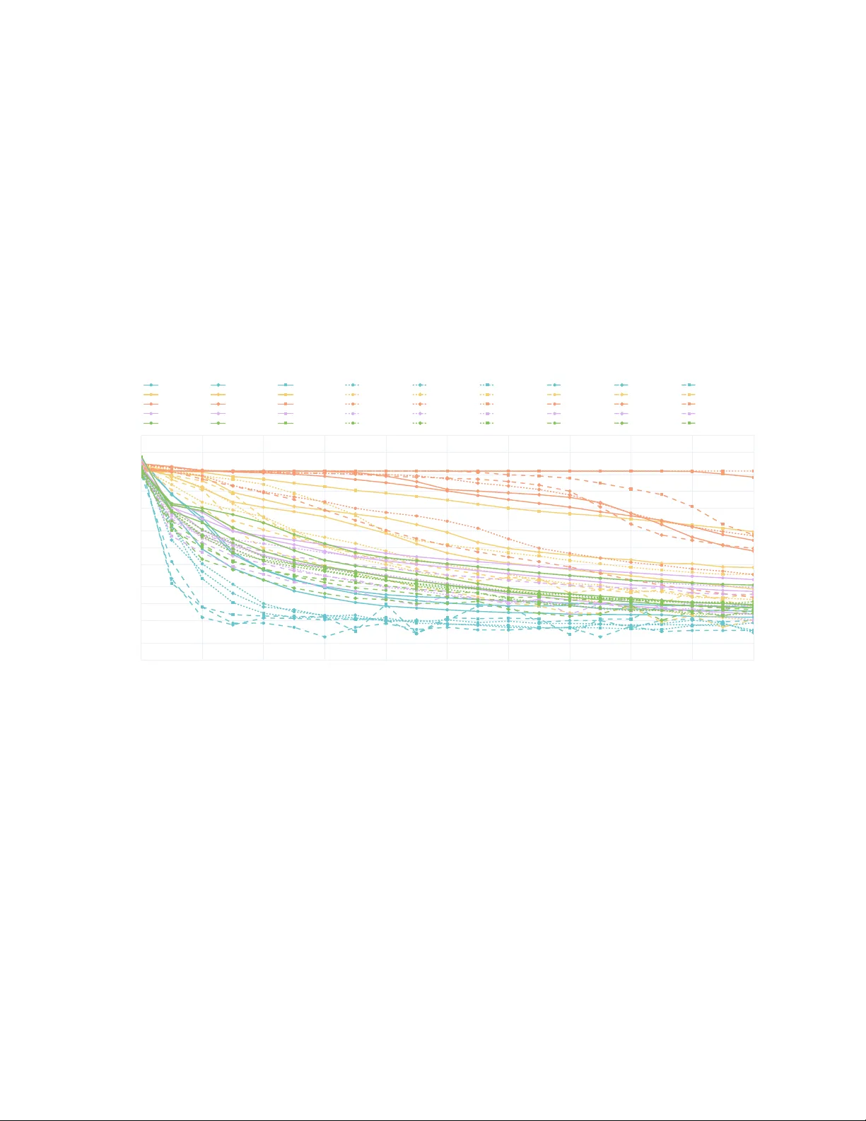
Loading comments...
Leave a Comment