Tractable bank capital structure: optimal control under Basel III constraints

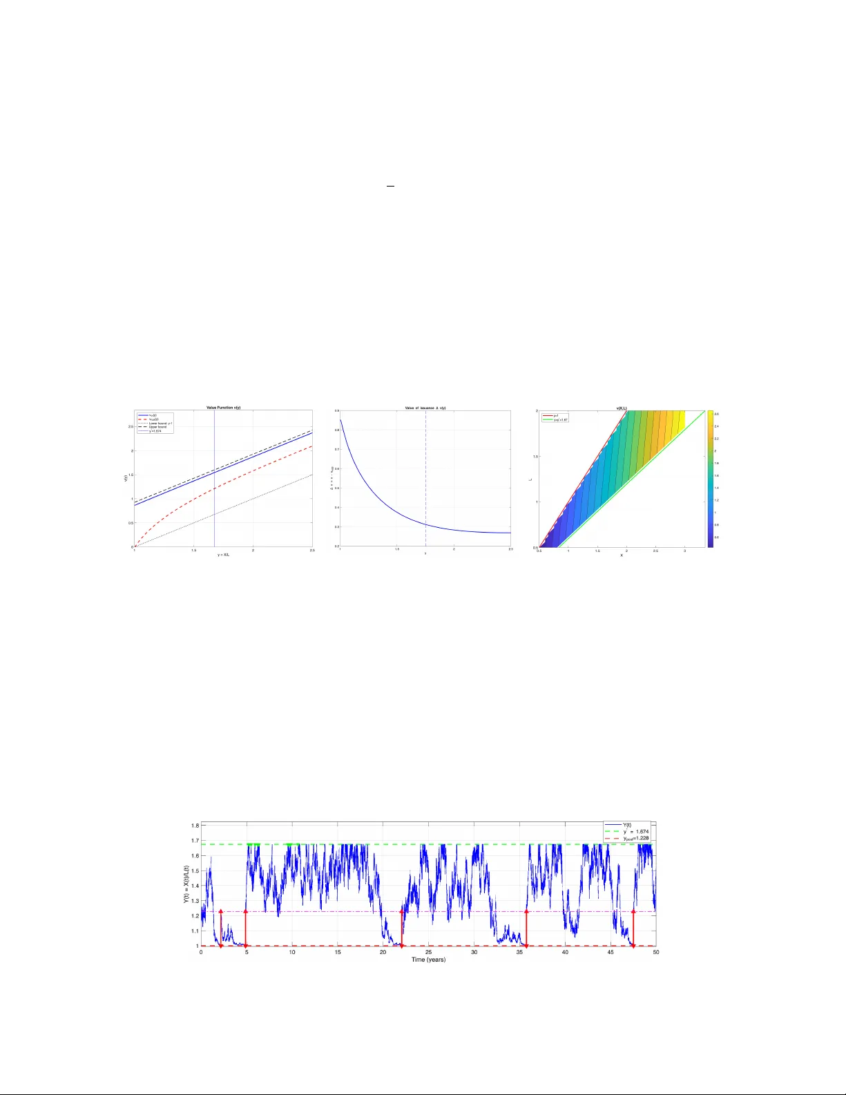
T ractable bank capital structure: optimal con trol under Basel I I I constrain ts Erhan Ba yraktar ∗ Etienne Chev alier † V athana Ly V ath ‡ Y uqiong W ang § Marc h 17, 2026 Abstract Banks m ust optimize risky inv estments, dividend pay outs, and capital structure under tigh t Basel I I I solvency and liquidity constraints, while costly equity issuance serv es as a distress-recov ery to ol. W e form ulate this as a sto chastic con trol problem that reduces the high-dimensional balance-sheet dynamics to a tractable one-dimensional pro cess in the lev erage ratio, with state-dep enden t inv estment limits. The resulting p olicy is simple and in terpretable: pay dividends at an upper reflec- tion barrier and, when needed, recapitalize only at the distress boundary , jumping to a unique target level. W e c haracterize these thresholds analytically and sho w their sensitivit y to regulatory parameters. F rom a regulatory viewpoint, w e solve an outer optimization problem that maps the efficien t frontier b et w een shareholder v alue and surviv al probability (via Mon te Carlo), with and without leverage caps. Results highligh t that tigh tening solvency requirements often yields the b est safety-profitabilit y trade-off. Key w ords : bank capital optimization, Basel I I I, optimal dividends, impulse and singular con trol, regulatory constrain ts, lev erage ratio, profitabilit y-safety fron tier. Con ten ts 1 In tro duction 2 2 Balance-sheet dynamics, regulatory constrain ts, and the bank’s optimiza- tion problem 4 3 Characterization of the optimal strategies 6 3.1 Analytical prop erties of the v alue function . . . . . . . . . . . . . . . . . . . 6 ∗ Departmen t of Mathematics, Universit y of Michigan, USA, erhan@umich.edu . Supp orted in pa rt b y the National Science F oundation and the Susan M. Smith Chair. † LaMME, Universite d’Evry , F rance, etienne.chevalier@univ-evry .fr. ‡ LaMME, ENSI IE, F rance, lyvath@ensiie.fr. § Departmen t of Mathematics, Universit y of Michigan, USA, yuqw@umich.edu. 1 3.2 Optimal dividend and capital issuance strategies . . . . . . . . . . . . . . . 9 4 Sensitivit y analysis and safet y-profitability fron tiers under regulation 9 4.1 V alue function and optimal strategies . . . . . . . . . . . . . . . . . . . . . 9 4.2 Sensitivit y to regulatory parameters . . . . . . . . . . . . . . . . . . . . . . 11 4.3 Regulatory parameter optimization . . . . . . . . . . . . . . . . . . . . . . . 12 5 App endix 17 1 In tro duction Banks contin uously balance three comp eting ob jectives: paying dividends to shareholders, taking on risky inv estmen ts to generate returns, and main taining sufficient capital and liquidit y buffers to satisfy regulators. Dividends are attractive to shareholders but reduce equit y; Risky in vestmen ts can raise profitabilit y but also increase the probabilit y of distress; recapitalization through new equity issuance can restore solvency , but it is typically costly due to flotation costs, dilution, and mark et frictions. These trade-offs are amplified b y regulatory requirements, suc h as Basel I I I’s Tier-1 capital ratio and Liquidity Co verage Ratio (LCR), whic h imp ose hard constrain ts on lev erage and liquid-asset holdings. In this pap er, we develop a tractable contin uous-time model of a bank’s optimal capital structure, dividend policy , and in v estment strategy under these tw o regulatory constraints. The bank collects dep osits (paying in terest rate r L ) and inv ests in risk-free and risky assets financed by dep osits and shareholders’ equity . The manager con trols the fraction π t in vested in the risky asset, cum ulative dividends, and the timing and size of equit y issuance, where issuance carries prop ortional costs κ and κ ′ . Solv ency and LCR requirements translate in to a state-dependent upper b ound π ( y ) on risky exposure, where y = X/L is the lev erage ratio (total assets o v er dep osits). The ob jectiv e is to maximize shareholders’ v alue — exp ected discoun ted dividends net of issuance costs — sub ject to bankruptcy when equit y hits zero. These regulatory constraints activ ely shap e the bank’s feasible strategies. As capital or liquidit y buffers deteriorate, the bank ma y b e forced to reduce risk taking, retain earnings, recapitalize at a cost, or liquidate. Issuance costs create a tension b et ween immediate p enalties and the v alue of av oiding distress. Dynamic mo dels of bank capital structure with costly recapitalization form a growing lit- erature. [18] study optimal equity c hoice under dela yed issuance. The effect of capital regulation on banks’ p ortfolio choices is studied in [19]; [14] and [4] examine ho w liquidit y and lev erage rules join tly drive capital structure, default risk, and refinancing. [4] in par- ticular deriv e a tw o-sided b oundary for dividends and issuance in a setting without hard regulatory distress triggers. Liquidit y is often treated as an exogenous buffer [9] or via runoff/haircut assumptions [2, 5, 10]; [10] argue that while the LCR reduces reliance on short-term funding, its optimal design remains op en. Early w orks on singular dividend 2 con trol include [6] and [15], while com bined singular-impulse and switching problems are studied in [21] and others. F rom a mathematical persp ectiv e, the problem is a com bined singular-impulse con trol prob- lem for diffusions: singular control for dividends (reflection barriers, [13]; [15]) and impulse con trol for recapitalization (jump structure, [12, 17]; [1]). A related corp orate finance model is studied in [7]. Extensions incorp orating in vestmen t/gro wth app ear in [8], [16], [11], and others. Our contribution adv ances this line in three key wa ys, with direct relev ance to sto c hastic optimization in OR. First, we em b ed Tier-1 solvency and LCR constraints (with haircuts and runoff ) in to the admissible set π ( y ). Exploiting homogeneity , the t w o-dimensional ( X , L ) problem reduces to a one-dimensional impulse-singular problem in lev erage ratio Y t = X t /L t . Prior banking mo dels t ypically remain tw o-dimensional, as they do not leverage the fact that both regu- latory ratios dep end solely on y . This reduction mak es the problem analytically tractable. Second, we fully characterize the v alue function analytically . It is the unique contin uous viscosit y solution to the v ariational inequalit y , satisfies linear gro wth, and—crucially—is conca ve in y . Concavit y , a staple of unconstrained dividend problems, survives despite state-dep enden t inv estment caps and forces a clean threshold geometry: dividends via reflection at a single upp er barrier y ∗ , and (when optimal) recapitalization only at the distress boundary y = 1 jumping to a unique target, see Theorem 3.1, which states the pap er’s main analytical result. This contrasts sharply with t wo-sided b oundaries in less- constrained settings (e.g., [4]) and extends classical reflection results (e.g., [15]) as w ell as com bined singular-impulse frameworks (e.g., [1]) to regulated inv estmen t environmen ts with dual state-dependent constrain ts. Third, w e obtain quantitativ e insights that are directly relev an t for regulation. W e explicitly c haracterize y ∗ and the p ost-issuance target, trace sensitivities to regulatory parameters a 1 (solv ency), a 2 (runoff ), a 3 (haircut), and quan tify the recapitalization option’s v alue. W e then form ulate and solv e a regulator’s problem—maximize bank v alue sub ject to a surviv al- probabilit y constraint ov er a finite horizon—with and without a no-leverage restriction ( π ≤ 1). Mon te Carlo ev aluation of the resulting P areto fron tier sho ws a 1 dominates in both regimes, implying capital-requirement tigh tening is often the most efficien t safety to ol, see Section 4.3. This regulator-facing optimization fills a gap in the sto c hastic-control banking literature and aligns with OR’s emphasis on computationally grounded p olicy analysis. The paper pro ceeds as follo ws. Section 2 details balance-sheet dynamics, constrain ts, and the one-dimensional reduction. In Section 3, w e first pro ve the viscosit y characterization and conca vity of the v alue function, using which we deriv e the explicit thresholds for issuance and dividends. Section 4 presents n umerical results on v alue/p olicy sensitivities and the regulator’s frontier. Pro ofs app ear in the Appendix 5. 3 2 Balance-sheet dynamics, regulatory constrain ts, and the bank’s optimization problem Let (Ω , F , P ) b e a probability space equipp ed with a filtration F = ( F t ) t ≥ 0 satisfying the usual conditions. All random v ariables and sto c hastic processes are defined on this probabil- it y space. Let W and B b e tw o correlated F -Bro wnian motions, with correlation co efficient c , i.e. d [ W , B ] t = cdt for all t . W e consider a bank whose liabilities consist of customer de- p osits, denoted b y L t at time t . W e assume that the pro cess L is gov erned by the following sto c hastic differential equation dL t = L t ( µ L dt + σ L dW t ) , L 0 = ℓ, (1) where σ L is a p ositiv e constan t and µ L := γ + r L , with γ ∈ R being the exogenous gro wth rate of the deposit and r L ≥ 0 the interest rate paid by the bank to its clien ts. The bank ma y inv est in a risk-free asset with a constan t interest rate r > 0 or in a risky asset whose v alue pro cess S solv es the follo wing sto c hastic differen tial equation dS t = S t ( µdt + σ dB t ) , S 0 = s, (2) where µ ∈ R , σ > 0. Let X t denote the bank’s total assets at time t , and let π t denote the fraction in vested in the risky asset. Accordingly , (1 − π t ) X t is inv ested in the risk-free asset and π t X t is inv ested in the risky asset b y the bank at time t . By the balance-sheet iden tity , we hav e X t = F t + L t ∀ t ≥ 0 , where F t corresp onds to shareholders’ equit y at time t . The manager of the bank con trols b oth the assets allo cation b et ween the risk-free and risky assets and the bank’s capital through equit y issuance and dividend pa ymen ts. W e then consider a con trol strategy b α = (( τ n ) n ∈ N ∗ , ( b ξ n ) n ∈ N ∗ , b Z , π ), where the F -adapted c´ adl´ ag nondecreasing pro cess b Z represen ts the total amount of dividend distributed, with b Z 0 − = 0. The non-decreasing sequence of stopping times ( τ n ) n ∈ N ∗ represen ts the decision times at whic h the manager decides to issue new capital, and b ξ n ∈ (0 , + ∞ ) whic h is F τ − n -measurable, represents amoun t of capital issue at τ n . The pro cess π is the prop ortion of the bank’s wealth in vested in the risky asset. The equit y process associated with a con trol b α then has the follo wing dynamics: ( dF t = − r L L t dt − d b Z t + (1 − π t ) X t r dt + π t X t ( µdt + σ dB t ) for τ i < t < τ i +1 F τ i = (1 − κ ) F τ − i + (1 − κ ′ ) b ξ i where κ ′ , κ > 0 are issuance cost parameters. More precisely , when issuing capital at time t , we assume that one has to pa y a cost proportional to the capital issued and κF t − is the cost due to comp ensation for existing (prior to the issue of capital) shareholders (against dilution). W e also assume that b ξ i is large enough to ensure that F τ i > F τ − i i.e. b ξ i > κ 1 − κ ′ F τ − i . 4 Otherwise, the manager would b e b etter off av oiding issuance and distributing dividends instead. The corresp onding w ealth pro cess X then solves      dX t = ((1 − π t ) r X t + π t µX t + γ L t ) dt + π t σ X t dB t + σ L L t dW t − d b Z t , for τ i < t < τ i +1 , X τ i = X τ − i + (1 − κ ′ ) b ξ i − κF τ − i (3) W e first define the bankruptcy time as the first time when the equity b ecomes negativ e: T b α = inf { t ≥ 0 : F t < 0 } W e assume that when the bankruptcy time is reac hed, the bank is liquidated immediately and ceases operations. W e fix a constan t shareholder’s discoun t rate ρ > 0. The sharehold- ers receive cum ulative dividends b Z until bankruptcy . A t capital issuance time τ n , a total amoun t of (1 − κ ′ ) b ξ n is added to the equity , while the dilution cost κF τ − n is extracted at issuance. Accordingly , the next issuance cashflow to the shareholders at τ n is b ξ n − κF τ − n . Giv en initial liability ℓ > 0 and initial w ealth x > 0, the shareholders’ present v alue under the p olicy b α is defined b y J b α ( ℓ, x ) = E l,x h Z T b α 0 e − ρt d b Z t − + ∞ X n =1 e − ρτ n ( b ξ n − κF τ − n )1 l { τ n ≤ T b α } i . W e no w in tro duce the regulatory constrain ts that reflects the institutional features of bank- ing. The first constraint is a solvency requirement, which reflects the ability of the bank to absorb losses without default. In our setting, the solvency ratio is the ratio of equit y to risky asset holdings. In our problem, it corresp onds to the ratio b etw een shareholders’ eq- uit y and its risky in vestmen ts F t π t X t ≥ a 1 for some a 1 ∈ (0 , 1). Equiv alently , by in tro ducing the leverage ratio Y t := X t L t , this condition can b e rewritten as 1 − 1 Y t ≥ a 1 π t . The second constrain t is the Liquidity Cov erage Ratio (LCR), defined as the ratio b et w een High Qualit y Liquid Assets (HQLA) and cash outflow during 30 days. The main cash outflo ws we consider are the potential run-off of proportion of retail dep osits, and we model the 30 − day net outflow as a fixed fraction a 2 ∈ (0 , 1) of liabilities, i.e., a 2 L t . W e assume that risk-free assets qualify fully as HQLA. In addition, we allow risky assets to contribute to HQLA only after applying a regulatory haircut as indicated in the Basel II I LCR framework [3]. In other words, a fraction a 3 ∈ (0 , 1) is excluded from HQLA. Hence, when the bank in vests a fraction π t in risky assets, the HQLA level is (1 − π t ) X t +(1 − a 3 ) π t X t = X t − a 3 π t X t . The liquidity constraints can therefore b e expressed as X t − a 3 π t X t a 2 L t ≥ 1 for all t ≥ 0 , or in terms of the lev erage ratio Y , 1 − a 2 Y t ≥ a 3 π t . 5 This leads us to introduce the function π defined on [1 , + ∞ ) by π ( y ) = min  1 a 1 (1 − 1 y ); 1 a 3 (1 − a 2 y )  . (4) The function π gives the regulatory upper b ound on the proportion of inv estment in risky assets. The set of admissible con trols, denoted b y b A , is defined b y b A = { b α = (( τ n ) n ∈ N ∗ , ( b ξ n ) n ∈ N ∗ , b Z , π ) : ∀ 0 ≤ t ≤ T b α , 0 ≤ π t ≤ π ( X t L t ) , ∀ n ≥ 1 : b ξ n > κ 1 − κ ′ F τ − n } . Hence, our v alue function is defined by b v ( ℓ, x ) = sup b α ∈ b A J b α ( ℓ, x ) for ( ℓ, x ) ∈ S := { ( ℓ, x ) ∈ [0 , + ∞ ) 2 : x ≥ ℓ } . (5) W e no w state a result that transforms our initial t wo-dimensional problem into a one- dimensional control problem in terms of the leverage ratio Y , whic h is also a natural state v ariable from a regulatory p ersp ectiv e. Prop osition 2.1 (Reduction to the leverage ratio) . L et α := (( τ n ) n ∈ N ∗ , ( ξ n ) n ∈ N ∗ , Z , π ) wher e ( τ n ) n ∈ N ∗ is an incr e asing se quenc e of stopping times, ( ξ n ) n ∈ N ∗ a se quenc e of p ositive F τ − n -me asur able r andom variables, and Z an incr e asing pr o c ess. Define the pr o c ess Y α as a solution of the fol lowing sto chastic differ ential e quation          d Y α t = ( Y α t [ µ ( π t ) − µ L ] + γ ) dt + π t Y α t σ dB t + σ L (1 − Y α t ) dW t − d Z t for τ n < t < τ n +1 Y τ n = (1 − κ ) Y τ − n + (1 − κ ′ ) ξ n + κ, wher e µ ( π ) = (1 − π ) r + π µ . Define the stopping time T α = inf { t ≥ 0 : Y α t < 1 } . We have b v ( ℓ, x ) = lv ( x ℓ ) , for al l ℓ > 0 and x ≥ ℓ , wher e v : [1 , ∞ ) → R is given by v ( y ) = sup α ∈A E y h Z T α 0 e − ρ L t d Z t − + ∞ X n =1 e − ρ L τ n ( ξ n − κ ( Y α τ − n − 1)) 1 l { τ n ≤ T α } i with ρ L := ρ − µ L . 3 Characterization of the optimal strategies In this section, w e study the v alue function and establish its analytical prop erties, and later use them to c haracterize the optimal strategies. 3.1 Analytical prop erties of the v alue function This subsection establishes the analytical prop erties of the v alue function, whic h underpin the structure of the optimal strategies later. Its main result is the v is the unique viscosity solution of the follo wing v ariational inequality:      0 = min { ρ L v ( y ) − sup 0 ≤ π ≤ π ( y ) L π v ( y ); v ′ ( y ) − 1; v ( y ) − H v ( y ) } , v (1) = max (0 , H v (1)) . (6) 6 where the impulse op erator H is defined by H φ ( y ) = sup ξ > κ 1 − κ ′ ( y − 1) h φ ((1 − κ ) y + (1 − κ ′ ) ξ + κ ) − ξ + κ ( y − 1) i , and the operator L π is defined b y L π φ ( y ) = 1 2  π 2 σ 2 y 2 + 2 π cσ σ L y (1 − y ) + σ 2 L (1 − y ) 2  φ ′′ + ( y [ µ ( π ) − µ L ] + γ ) φ ′ . with µ ( π ) = (1 − π ) r + π µ . W e first observe that for any b ounded stopping time θ , the v alue function v satisfies the follo wing dynamic programming principle (DPP): v ( y ) = sup α ∈A E y h Z θ 0 e − ρ L t d Z t − X τ n ≤ θ e − ρ L τ n ( ξ n − κ ( Y α τ − n − 1)) + e − ρ L θ v ( Y α θ ) i . (7) 3.1.1 Lo w er and upp er b ounds for the v alue function W e introduce notation that will b e useful in the analysis. Recall that the bank allo cates a fraction π t of its assets to the risky asset, and the instan taneous exp ected return is µ ( π t ) = r + ( µ − r ) π t . Since µ is affine in π t and the regulatory constraints tell us 0 ≤ π t ≤ π ( y ). µ ( π ) is th us maximized at an endp oin t. W e define the drift-maximizing strategy b y π ∗ ( y ) = π ( y )1 l { µ ≥ r } , and the corresp onding maximized instantaneous exp ected return by µ ∗ ( y ) := r + π ∗ ( y )( µ − r ) = max { (1 − π ) r + π µ : 0 ≤ π ≤ π ( y ) } . W e emphasize here that π ∗ is not necessarily optimal for the full con trol problem, since optimalit y also dep ends on the correlation and volatilit y parameters, as well as the issuance and dividend strategies through the v ariational inequality . W e refer to π ∗ as the m yopic strategy for the rest of the pap er. Recall that the upp er b ound π ( y ) = min  1 a 1 (1 − 1 y ); 1 a 3 (1 − a 2 y )  increases in y , and it con verges as y → ∞ to lim y →∞ π ( y ) = 1 max( a 1 ,a 3 ) =: 1 ¯ a . It follo ws that sup y ≥ 1 µ ∗ ( y ) =    r , µ ≤ r , µ +(1 − ¯ a ) r ¯ a , µ > r. In particular, π (1) = 0, so at y = 1 the bank can only inv est in risk-free assets. Therefore, w e assume r > r L , so that the ratio pro cess has a p ositiv e drift at y = 1 and the problem remains economically meaningful. W e now imp ose a parameter restriction ensuring that the discounting dominates the maximal gro wth p ermitted b y regulation, whic h guarantees the well-posedness of the problem. Prop osition 3.1. If ρ < max( µ L , r + ( µ − r ) + ¯ a ) , we have v ( y ) = + ∞ on [1 , + ∞ ) . F or an y initial state y ≥ 1, the bank can liquidate immediately by pa ying dividends up to bankruptcy . This immediately yields the low er b ound: v ( y ) ≥ y − 1 , for y ≥ 1 . (8) W e next construct an upper b ound for v , sho wing that the v alue grows at most linearly . This relies on the following t wo results. 7 Prop osition 3.2. L et φ ∈ C 2 ([1 , + ∞ )) such that min( φ (1) , φ (1) − H φ (1)) ≥ 0 and min " ρ L φ ( y ) − sup π ∈ [0 ,π ( y )] L π φ ( y ); φ ′ ( y ) − 1; φ ( y ) − H φ ( y ) # ≥ 0 , for any y > 1 (9) then v ≤ φ on [1 , + ∞ ) . Corollary 3.1. L et y ∈ [1 , + ∞ ) . We have y − 1 ≤ v ( y ) ≤ y + 1 ρ L max ( − ρ L , A + γ , B + γ ) , wher e the p ar ameters A and B ar e given by A :=  r + ( µ − r ) + a 3 − ρ  ˆ y − a 2 ( µ − r ) + a 3 B :=  r + ( µ − r ) + a 1 − ρ  + ˆ y −  r + ( µ − r ) + a 1 − ρ  − − ( µ − r ) + a 1 , with the r e gime switching p oint ˆ y = a 3 − a 1 a 2 a 3 − a 1 . In p articular, if − ρ L ≥ max ( A, B ) + γ , v ( y ) = y − 1 , the optimal p olicy is to imme diately distribute dividends up to b ankruptcy. By Prop osition 3.2 and Corollary 3.1, we exclude b oth cases where the v alue function blow up, and the degenerate case where immediate liquidation is alwa ys optimal. Accordingly , throughout the rest of the paper w e assume that the parameters satisfy: ρ > max( µ L , r + ( µ − r ) + ¯ a ) and − ρ L < max( A, B ) + γ . (10) 3.1.2 Viscosit y c haracterization of the v alue function W e first state the contin uity of v , whic h is needed for b oth the viscosity framework and the stable c haracterization of the free b oundaries. W e then show in Prop osition 3.3 that the v alue function is uniquely characterized as the solution of the v ariational inequality . Prop osition 3.3 (Viscosity characterization of the v alue function) . The value function v is the unique c ontinuous function on [1 , + ∞ ) that satisfies a line ar gr owth c ondition and is a visc osity solution of (6) . The key structural prop erty of the v alue function is concavit y , because it shap es the ge- ometry of the optimal control regions. Economically , conca vity of v indicates diminishing marginal v alue of capital: an additional unit of y is most v aluable near bankruptcy , which leads to a single-threshold type of dividend structure. Prop osition 3.4 (Conca vity of the v alue function) . The value function v is c onc ave on [1 , ∞ ) . Finally , we define the con tinuation, dividend, and issuance regions, and establish in terior regularit y of v , which yields a classical solution in the contin uation region. This is not merely tec hnical: it pro vides the smo oth-fit conditions used to compute the dividend barrier, and it supp orts the n umerical analysis. 8 Corollary 3.2. The value function v is C 1 on { y > 1 : v ( y ) > H v ( y ) } . Define the issuanc e r e gion K , dividend r e gion D , and the c ontinuation r e gion C by K := { y ≥ 1 , v ( y ) = H v ( y ) } (11) D = in t ( { y ≥ 1 , v ′ ( y ) = 1 } ) , (12) C = { y > 1 : v ( y ) > H v ( y ) , D + v ( y ) > 1 } . (13) We have C op en and K ∩ D = ∅ . F urthermor e, v is C 2 on the op en set C ∪ in t( D ) , and the HJB e quation ρ L v ( y ) − sup 0 ≤ π ≤ π ( y ) L π v ( y ) = 0 , y ∈ C holds in the classic al sense. 3.2 Optimal dividend and capital issuance strategies In this section, we translate the v ariational inequality into explicit c haracterizations of the optimal strategies, whic h constitutes the pap er’s main structural result. First, dividends are optimal when retaining one more unit of capital is no more v aluable than paying it out. The concavit y of the v alue function means that once paying dividends is optimal, it remains optimal for all larger y , which implies a single barrier structure. The same conca vity argument also gov erns capital issuance. Theorem 3.1 shows that the optimal strategy has a simple t wo-sided structure: dividends are paid at an upp er barrier, while recapitalization, when optimal, is triggered at the distress b oundary and jumps to a unique p ost-issuance target. Theorem 3.1. Optimal dividend and c apital issuanc e str ate gy. The optimal str ate gy is char acterize d as fol lows. (i) The e quation ρ L v ( y ) = γ − ( µ L − µ ∗ ( y )) y a dmits a unique solution y ∗ on [1 , + ∞ ) . In addition, y ∗ satisfies 1 ≤ y ∗ < ρ L + γ ρ − µ ∗ ( y ∗ ) , and the dividend r e gion is of the form D = [ y ∗ , + ∞ ) . (ii) K ⊂ { 1 } . Mor e over, if K  = ∅ , then v ′ (1 + ) > 1 1 − κ ′ , and ther e exists a unique p ost- issuanc e tar get y ∗ post such that v ′ ( y ∗ post ) = 1 1 − κ ′ . The c orr esp onding optimal issuanc e amount is ξ ∗ = y ∗ post − 1 1 − κ ′ . Final ly, the value function at y = 1 satisfies v (1) = v ( y ∗ post ) − 1 1 − κ ′  y ∗ post − 1  . 4 Sensitivit y analysis and safet y-profitabilit y fron tiers under regulation 4.1 V alue function and optimal strategies 1 W e b egin by plotting the v alue function v and comparing it with the b enchmark case where equity issuance is not allo w ed, denoted b y v H J B . The function v H J B represen ts the 1 The numerical results in this section were generated using scripts av ailable on GitHub at https:// github.com/yuqiongwang/bank_capital_structure 9 v alue function without the p ossibilit y of issuing capital, and it solv es the follo wing singular con trol problem: 0 = min { ρ L v ( y ) − sup 0 ≤ π ≤ π ( y ) L π v ( y ); v ′ ( y ) − 1 } , v (1) = 0 . In the n umerical exp erimen ts, w e use the following baseline parameters: r = 0 . 01 , µ = 0 . 04 , µ L = 0 . 03 , ρ = 0 . 12 , σ = 0 . 08 , σ L = 0 . 03 , c = 0 . 20 , γ = 0 . 01 together with issuance costs κ = 0 . 01 and κ ′ = 0 . 02. Figure 1 sho ws that the incremen tal v alue generated b y the option of issuing is largest at y = 1 and decreases monotonically with y . In other w ords, the flexibility to recapitalize is most useful when the bank is close to bankruptcy and b ecomes less relev an t when the bank is well-capitalized. F or completeness, w e also plot the v alue function expressed in the original ( x, l ) − coordinate. (a) The v alue function v ( y ) (b) v ( y ) − v H J B ( y ) (c) Contour in ( x, l ) Figure 1: The v alue function of y and ( x, l ). W e illustrate the strategy in Figure 2 by sim ulating a single sample path starting from y 0 = 1 . 2, with a dividend barrier y ∗ = 1 . 674 and a p ost-issuance target y ∗ post = 1 . 228, o ver a horizon of 50 y ears. The path sho ws the expected t w o-sided con trol structure: each time the state hits the issuance b oundary y = 1, it jumps up ward by a fixed size in to the in terior of the contin uation region. Eac h time the state reac hes the dividend region at y ∗ it is reflected back in to the con tinuation region. In this simulation, the cumulativ e issuance is 1 . 63 and the cumulativ e dividend pa y out is 4 . 78, as sho wn in Figure 3. Figure 2: T ra jectory from y 0 = 1 . 2 of 50 y ears 10 Figure 3: T otal capital and dividend of 50 years 4.2 Sensitivit y to regulatory parameters W e next study ho w the optimal dividend b oundary y ∗ and the relative v alue of issuance resp ond to c hanges in the regulatory parameters a 1 , a 2 and a 3 . F rom the mo del’s p ersp ec- tiv e, ( a 1 , a 2 , a 3 ) only en ter through the state-dep endent inv estment cap π ( y ). Changing these parameters affects the drift and v olatility of the underlying pro cess Y by altering the admissible inv estmen t cap, and hence the feasible v alues of π ( y ) ≤ π ( y ). The dividend barrier y ∗ reflects the balance b etw een curren t dividend pay outs and maintaining a future buffer under the constrain t dynamics. The issuance v alue ∆ v /v increases when the con- strain t mak es it more lik ely to hit bankruptcy , and it decreases when the process tends to a void hitting the lo w er boundary , thus making recapitalization less attractiv e. The key structure is the minimum op erator that has a switching p oin t ˆ y > 1, whic h induces a t w o-regime inv estment cap. With our curren t baseline parameters ( a 1 , a 2 , a 3 ) = (0 . 045 , 0 . 05 , 0 . 3), w e hav e ˆ y = 1 . 168. When 1 < y ≤ ˆ y , the inv estmen t cap π ( y ) = 1 a 1 (1 − 1 y ) (solv ency-dominated), and when y > ˆ y we hav e π ( y ) = 1 a 3 (1 − a 2 y ) (liquidity-dominated). In addition, ev ery issuance even t mo ves the bank directly to the p ost issuance state y ∗ post = 1 . 228 in the liquidity-dominated region. Thus, an issuing ev ent not only raises capital but ma y also mov e the bank in to a different regulatory regime through the risky inv estment cap. The n umerical results are rep orted in T able 1. Keeping all other parameters fixed, we ev aluate the model at the reference level y 0 = 1 . 2 and v ary one regulatory parameter at a time. W e rep ort ( i ) the dividend threshold y ∗ and ( ii ) the relativ e v alue of issuance: ∆ v v ( y 0 ) := v − v H J B v ( y 0 ) , (14) whic h measures the fraction of the v alue function due to the p ossibility of issuance. It reflects both the lik eliho o d of hitting the bankruptcy b oundary and the contin uation v alue generated near the p ost-issuance target y ∗ post . 11 T able 1: Sensitivity to ( a 1 , a 2 , a 3 ) at y 0 = 1 . 2. a 1 a 1 y ∗ ∆ v v (1 . 2) 0.045 1.674 0.5229 0.05 1.699 0.5235 0.06 1.753 0.5245 0.07 1.814 0.5256 0.08 1.882 0.5276 0.09 1.957 0.5304 0.1 2.041 0.5357 0.11 2.134 0.5438 0.12 2.236 0.5545 a 2 a 2 y ∗ ∆ v v (1 . 2) 0.05 1.674 0.5229 0.06 1.667 0.5198 0.08 1.653 0.5136 0.09 1.646 0.5105 0.1 1.639 0.5073 0.12 1.625 0.5008 0.15 1.604 0.4909 0.18 1.583 0.4806 0.2 1.569 0.4735 a 3 a 3 y ∗ ∆ v v (1 . 2) 0.15 1.895 0.8074 0.2 1.885 0.7144 0.25 1.710 0.6089 0.3 1.674 0.5229 0.35 1.414 0.4882 0.4 1.316 0.4659 0.45 1.259 0.4443 0.5 1.221 0.4243 0.55 1.193 0.4060 First, we observ e that increasing a 1 from the baseline v alue 0 . 045 to 0 . 12 leads to a large increase in y ∗ from 1 . 674 to 2 . 236. A t the same time, the relative gain rises mo derately . a 1 en ters only through the first regime 1 a 1 (1 − 1 y ) and increasing a 1 lo wers this cap for all y , shrinks the feasible set in size throughout that regime. Consequen tly , the bank is motiv ated to adopt a more conserv ativ e strategy by retaining earnings and building a larger capital buffer b efore pa ying dividends, and th us the free b oundary y ∗ shifts up ward. Similarly , solvency tightening makes it more lik ely to hit the bankruptcy b oundary , and recapitalization b ecomes more attractive, so the relative v alue of issuance also increases. Ho wev er, the relativ e issuance v alue increases only mo derately compared to the large shift in y ∗ as a 1 has no influence in the liquidit y-dominated region. As a 2 rises from 0 . 05 to 0 . 2, y ∗ falls from 1 . 674 to 1 . 569, and ∆ v v (1 . 2) falls from 0 . 5229 to 0 . 4735. The parameter a 2 reduces the contin uation v alue at y ∗ post , and thus issuance is less attractiv e, though still feasible. Similarly , the contin uation v alue is less sensitiv e to extra capital buffers. And th us v ′ drops so oner tow ards 1 and y ∗ decreases. In addition, the volatilit y decreases for admissible v alues of π in the region of interest. It is then less lik ely to hit y = 1, whic h again supp orts a smaller y ∗ . Increasing a 3 from 0 . 15 to 0 . 55 has a similar effect: the dividend b oundary falls from 1 . 895 to 1 . 193, and ∆ v v (1 . 2) changes from 0 . 8074 to 0 . 4060. This is because a 3 w orks similarly to a 2 on the in vestmen t cap in the liquidit y-dominated region, whic h scales the whole cap uniformly . 4.3 Regulatory parameter optimization F rom a regulatory persp ectiv e, it is natural to push the parameters a 1 , a 2 , a 3 as high as p ossible to increase resilience. Doing so, ho wev er, comes at the cost of reduced profitabil- it y for the bank. The ov erall health of a financial institution cannot b e assessed solely through solv ency considerations: it must balance the in terests of regulators, shareholders, and dep ositors. Motiv ated by this trade-off, we in tro duce a metric to quantify the ov erall health of the bank. First, the bank should op erate with lo w default risk, or at least with 12 limited exp osure to financial stress. Since equit y issuance is triggered only at the solvency b oundary , we in terpret a b oundary hit as a stress even t and define the asso ciated hitting time: τ := inf { t ≥ 0 : Y t < 1 } and require the probability of av oiding suc h a stress ev ent ov er a reference horizon to b e sufficien tly high. On the other hand, for any fixed regulatory triple ( a 1 , a 2 , a 3 ), the bank resp onds optimally b y solving the v ariational inequality (6). This leads to the following optimization problem with restrictions: max { ( a 1 ,a 2 ,a 3 ) } v ( y 0 ) s.t. P ( τ ≥ T ) ≥ η for some probability threshold η and reference time T . In this numerical illustration, w e set T = 5. W e numerically approximate the solution of this problem by ev aluating all com binations in the following parameter grids: a 1 ∈ { 0 . 045 , 0 . 05 , 0 . 06 , 0 . 07 , 0 . 08 , 0 . 09 , 0 . 10 , 0 . 11 , 0 . 12 } , a 2 ∈ { 0 . 05 , 0 . 06 , 0 . 08 , 0 . 09 , 0 . 10 , 0 . 12 , 0 . 15 , 0 . 18 , 0 . 2 } , a 3 ∈ { 0 . 15 , 0 . 20 , 0 . 25 , 0 . 3 , 0 . 35 , 0 . 4 , 0 . 45 , 0 . 5 , 0 . 55 } , excluding parameter com binations that violate the feasibility conditions (10). F or eac h parameter triple, W e ev aluate the mo del at y 0 = 1 . 2, using 1 , 000 Monte Carlo simulations. In our model, π is the proportion in vested in risky assets, π > 1 corresponds to a lev eraged p osition, and π ∈ [0 , 1] corresp onds to a no-borrowing long p osition. Although allowing π > 1 is natural in theoretical in vestmen t optimization problems, it makes more sense for real-w orld banks to hav e leverage constraints. F or this reason, and as a robustness c heck, w e study tw o cases: one without any additional restriction on π , and one with the leverage constrain t π ≤ 1. 4.3.1 Case without a leverage restriction In this case, we ha v e 486 parameter triples in total that are feasible. W e first plot the pairs ( P ( τ ≥ 5) , v ( y 0 )) generated by all the feasible parameter triples, and illustrate the trade-off b et ween profit and safety . W e call a triple ( a 1 , a 2 , a 3 ) efficien t if no other triple yields b oth a higher v alue v ( y 0 ) and a higher surviv al probabilit y P ( τ ≥ 5). W e indicate these p oin ts in the plot in Figure 4 and sa y that they lie on the P areto efficient frontier, and w e further report these points in T able 2. On the frontier, an y attempt to increase the surviv al probability must come at a cost in the v alue function, and vice v ersa. F or any target surviv al probabilit y η , the optimal regulatory c hoice m ust lie on this frontier. 13 a 1 a 2 a 3 y ∗ v ( y 0 ) P ( τ ≥ T ) 0.12 0.18 0.3 2.069 0.8711 0.927 0.12 0.05 0.3 2.236 0.9948 0.923 0.11 0.06 0.3 2.122 0.9983 0.895 0.11 0.05 0.3 2.134 1.0079 0.868 0.1 0.05 0.3 2.041 1.0198 0.848 0.09 0.05 0.3 1.957 1.0304 0.754 0.08 0.05 0.3 1.882 1.0400 0.680 0.07 0.05 0.3 1.814 1.0487 0.597 0.06 0.05 0.3 1.753 1.0565 0.486 0.05 0.05 0.3 1.699 1.0634 0.433 0.045 0.05 0.3 1.674 1.0666 0.336 T able 2: Pareto fron tier without restriction Figure 4: Optimization without restriction The Pareto fron tier contains 11 p oin ts, and in terestingly , the frontier is primarily driven b y a 1 and almost alwa ys selects the same pair of liquidity parameters ( a 2 , a 3 ) = (0 . 05 , 0 . 3), and it seems to b e most sensitiv e to the solv ency parameter a 1 . Along those frontier p oin ts, increasing a 1 raises the dividend barrier substantially from 1 . 674 to 2 . 236, and this, in turn, affects the surviv al probability: P ( τ ≥ T ) rises from 0 . 336 to 0 . 923 as a 1 increases o ver the curve, while v ( y 0 ) decreases only sligh tly . In other w ords, tigh tening the solv ency parameter a 1 is the most efficient wa y to increase safety while not losing to o muc h v alue in our optimization, whereas altering a 2 , a 2 generally leads to dominated outcomes. In addition, the fron tier reveals some drastic b eha vior at high safet y levels. T o push beyond P ( τ ≥ T ) ≈ 0 . 923 one needs to increase a 2 sharply from 0 . 05 to 0 . 18, but reducing v ( y 0 ) to 0 . 8711. The gain in safety at this point thus b ecomes v ery expensive and requires v ery restrictiv e liquidit y regulations, whereas most of the impro vemen t in probability can b e ac hieved b y increasing a 1 only . Within our mo del, tightening requiremen ts b eyond this p oin t app ears inefficient, as it yields only a marginal safet y gain at a substantial cost in v alue. T able 3: Optimal regulatory parameters without restriction η a ∗ 1 a ∗ 2 a ∗ 3 y ∗ v ( y 0 ) P ( τ ≥ T ) 0.8 0.1 0.05 0.3 2.041 1.0198 0.848 0.9 0.12 0.05 0.3 2.236 0.9948 0.923 Fix η ∈ (0 , 1). Maximizing v ( y 0 ) under the constrain t P ( τ ≥ T ) ≥ η selects an optimal p oin t on the Pareto frontier, and typical choices of η could b e 0 . 8 , 0 . 9, rep orted in T able 3. In this subsection we tak e η = 0 . 8. Using the resulting optimized parameters, we sim ulate six representativ e banks with different starting p oin ts y 0 ’s ov er a 50 − year horizon. F or eac h initial condition, w e run 1 , 000 Monte Carlo tra jectories and compute the av erage cum ulative issuance and av erage cumulativ e dividends ov er the full horizon. In addition, 14 w e rep ort the Sharp e ratio of the net profit, E [net pay off] /σ (net pa yoff), to examine the risk-adjusted profitability of the bank. Here, σ ( · ) is the standard deviation. W e see a clear monotonic pattern in the initial health y 0 : as the bank is better capitalized, the exp ected accumulated dividends increase (from ab out 5 . 05 at y 0 = 1 . 05 to ab out 5 . 32 at y 0 = 1 . 30), and the Sharp e ratio also increases mo destly (from 1 . 87 to 1 . 95). This is consisten t with the fact that a well-capitalized bank reaches the dividend region so oner, and the increase in the Sharp e ratio indicates that the higher net pay off is not driven solely b y greater risk exp osure. In contrast, the expected cum ulative issuance decreases with y 0 (from 1 . 41 to 1 . 14), with the marginal reduction becoming smaller once y 0 is sufficiently high. T able 4: Monte Carlo simulation for 6 banks o ver 50 years without restriction y 0 E [T otal issuance] E [T otal dividend] Sharpe ratio 1.05 1.4077 5.0537 1.8698 1.1 1.2853 5.0502 1.8965 1.15 1.2311 5.0812 1.8757 1.2 1.1917 5.1485 1.8991 1.25 1.1598 5.2062 1.9138 1.3 1.1376 5.3152 1.9477 4.3.2 Case with the leverage restriction π ≤ 1 Under the restriction π ≤ 1, there are 729 feasible parameter triples. W e rep ort the p oin ts on the P areto fron tier in T able 5 and plot all pairs of ( P ( τ ≥ 5) , v ( y 0 )) in Figure 5. W e observ e that the v alue functions is substantially low er compared to the unrestricted case, and the P areto frontier is mainly affected b y the parameter a 1 . How ever, the optimiza- tion problem b ecomes degenerate in the sense that there are only 9 p oin ts on the Pareto fron tier in Figure 5, generated b y 9 v alues of a 1 . In effect, the v alue function is insensitiv e to the liquidity parameters ov er this range. How ever, increasing a 1 pushes the dividend b oundary higher and reduces the v alue function from 0 . 3357 to 0 . 2664, while deliv ering a large impro vemen t in surviv al probability . F or our choice of a 2 ≤ 0 . 2 , a 3 ≤ 0 . 55, the liquidit y cap satisfies 1 a 3 (1 − a 2 y ) ≥ 1 . 455 > 1 for all y ≥ 1. Th us, throughout the entire liquidit y-dominated region, π ≥ 1. Under the additional restriction π ≤ 1, the liquidit y con- strain ts nev er bind. This sho ws our earlier conclusion — that the parameter optimization problem is most sensitive to the solv ency constraint parameter a 1 — is robust. Differen t a 2 , a 3 parameters pro duce small differences in the estimated surviv al probabilit y , although they should not affect the con trol problem in this regime. Since these differences sho w no systematic monotonicity , they are most likely due to Monte Carlo noise. 15 a 1 a 2 a 3 y ∗ v ( y 0 ) P ( τ ≥ T ) 0.12 0.05 0.25 1.175 0.2664 0.860 0.11 0.08 0.25 1.164 0.2766 0.796 0.1 0.08 0.35 1.152 0.2867 0.724 0.09 0.08 0.15 1.141 0.2965 0.619 0.08 0.2 0.35 1.131 0.3059 0.507 0.07 0.06 0.4 1.121 0.3151 0.388 0.06 0.2 0.3 1.111 0.3237 0.264 0.05 0.09 0.4 1.102 0.3318 0.181 0.045 0.08 0.15 1.097 0.3357 0.134 T able 5: Pareto fron tier with π ≤ 1. Figure 5: Optimization with π ≤ 1. In contrast to the unrestricted case, there is no feasible parameter set achieving η ≥ 0 . 9 an ymore. W e therefore select the parameters that give η = 0 . 8, as shown in T able 6. T able 6: Optimal regulatory parameters with π ≤ 1. η a ∗ 1 a ∗ 2 a ∗ 3 y ∗ v ( y 0 ) P ( τ ≥ T ) 0.8 0.12 0.05 0.25 1.175 0.2664 0.86 As in the unconstrained case, we sim ulate the profitability of 6 banks restricted to π ≤ 1 with 1 , 000 Mon te Carlo tra jectories. The same monotonic relationship betw een profitabil- it y and the initial capitalization ratio is preserved. Compared to the unrestricted case, the lev erage cap substan tially reduces profitability: the accumulated dividends drop from 5 . 05 – 5 . 32 to 1 . 05 – 1 . 28, a reduction of roughly 75% – 80% reduction, but the total issuance also falls b y around 45% – 53%. Interestingly , the Sharp e ratios of the net gain are higher under the restriction: around 2 . 45 to 2 . 97 compared to 1 . 87–1 . 95 without restriction. Eco- nomically , imp osing the leverage tightens the distribution of the net profits, and it reduces the v ariance more than it reduces the mean. Th us, risk-adjusted profitabilit y improv es ev en though the absolute net pay off s are low er. T able 7: Monte Carlo simulation for 6 banks o ver 50 years with π ≤ 1 y 0 E [T otal issuance] E [T otal dividend] Sharpe ratio 1.05 0.6765 1.0465 2.4530 1.1 0.6425 1.0855 2.5124 1.15 0.6307 1.1365 2.6160 1.2 0.6261 1.1822 2.7263 1.25 0.6257 1.2318 2.8472 1.3 0.6257 1.2818 2.9684 16 5 App endix Pro of of Prop osition 2.1 Pr o of. Let ( l, x ) ∈ S \ { 0 } and b α = (( τ n ) n ∈ N ∗ , ( b ξ n ) n ∈ N ∗ , b Z , π ) ∈ A . W e define an increasing and c` adl` ag pro cess by Z t = Z t 0 L − 1 u d b Z t for t ≥ 0. Define a sequence of F τ n -measurable random v ariables by ξ n = b ξ n L τ n for n ∈ N ∗ . Using the iden tities F τ − n = X τ − n − L τ n = ( Y τ − n − 1) L τ n , d ˆ Z t = L t d Z t , we can write b J b α ( l, x ) = E l,x h Z T b α 0 e − ρt L t d Z t − ∞ X n =1 e − ρτ n L τ n ( ξ n − κ ( Y τ − n − 1))1 l { τ n ≤ T b α } i . Since the pro cess L is a geometric Brownian motion, it admits the representation L t = l exp  µ L − 1 2 σ 2 L  t + σ L W t  . Define a pro cess M by M t := L t l e − µ L t = exp( σ L W t − 1 2 σ 2 L t ), then M is a p ositiv e martingale. Substituting L t = l e µ L t M t in to the expression of b J , we obtain b J b α ( l, x ) = l E l,x h Z T b α 0 e − ρ L t M t d Z t − ∞ X n =1 e − ρ L τ n M τ n ( ξ n − κ ( Y τ − n − 1))1 l { τ n ≤ T b α } i . Moreo ver, by integration b y parts applied to the martingale M and the finite-v ariation pro cess R t 0 e − ρ L s d Z s , we obtain E l,x [ Z T b α 0 e − ρ L t M t d Z t = E [ M T b α Z T b α 0 e − ρ L t d Z t ] . F or each impulse term, the martingale prop erty of M yields E h e − ρ L τ n M τ n ( ξ n − κ ( Y τ − n − 1))1 l { τ n ≤ T b α } i = E h e − ρ L τ n E [ M T b α |F τ n ]( ξ n − κ ( Y τ − n − 1))1 l { τ n ≤ T b α } ] i = E h e − ρ L τ n M T b α ( ξ n − κ ( Y τ − n − 1))1 l { τ n ≤ T b α } i Consequen tly , w e can write the pa y off as b J b α ( l, x ) = l E l,x h M T Z T b α 0 e − ρ L t d Z t − ∞ X n =1 e − ρ L τ n ( ξ n − κ ( X b α τ − n L τ − n − 1))1 l { τ n ≤ T b α } ! i . W e no w in tro duce a new probabilit y measure P ∗ on F t b y d P ∗ d P   F t = M t . Under P ∗ , the pro cesses W ∗ and B ∗ defined by W ∗ t := W t − σ L t, B ∗ t := B t − cσ L t 17 are standard Bro wnian motions with correlation coefficient c . W e may therefore express the dynamics in terms of ( W ∗ , B ∗ ). Let Y b α denote the leverage ratio defined by Y b α t := X b α t L t . F or τ n < t < τ n +1 , Itˆ o’s form ula giv es, d Y b α t = dX b α t L t − X b α t dL t ( L t ) 2 + X b α t d ⟨ L ⟩ t ( L t ) 3 + d ⟨ X b α , L − 1 ⟩ t =  Y b α t [(1 − π t ) r + π t µ ] + γ  dt + π t σ Y b α t + σ L dW t − d Z t − Y b α t µ L dt − σ L Y b α t dW t + σ 2 L Y b α t dt − cπ t cσ σ L Y b α t dt − σ 2 L dt =  Y b α t  (1 − π t ) r + π t µ − µ L + σ 2 L − cπ t σ σ L  + γ − σ 2 L  dt + π t Y b α t σ dB t + σ L (1 − Y b α t ) dW t − d Z t . By Girsanov’s Theorem, under the measure P ∗ , the process Y b α t satisfies d Y b α t = ( Y α t [(1 − π t ) r + π t µ − µ L ] + γ ) dt + π t Y b α t σ d ( B t − cσ L t ) + σ L (1 − Y b α t ) d ( W t − σ L t ) − d Z t =  Y b α t [(1 − π t ) r + π t µ − µ L ] + γ  dt + π t Y b α t σ d ( B ∗ t ) + σ L (1 − Y b α t ) d ( W ∗ t ) − d Z t for τ n < t < τ n +1 . Moreo ver, at issuance times τ n , we hav e X τ n = X τ − n + (1 − κ ′ ) b ξ τ n − κF τ − τ n . Using F τ − n = ( Y b α τ − n − 1) L τ n and b ξ τ n = ξ τ n L τ n , this becomes X τ n = Y b α τ − n L τ n + (1 − κ ′ ) ξ τ n L τ n − κ ( Y b α τ − n − 1) L τ n . Equiv alently , Y b α τ n = (1 − κ ) Y b α τ − n + (1 − κ ′ ) ξ τ n + κ . W e define the control set by A : A = { α := (( τ n ) n ∈ N ∗ , ( ξ n ) n ∈ N ∗ , Z , π ) : ∀ t ≥ 0 : 0 ≤ π t < π ( Y α t ) , ∀ n ≥ 0 : ξ n > κ 1 − κ ′ ( Y α τ − n − 1) } . F or each b α ∈ b A , there exists an α ∈ A such that Y b α = Y α . Finally , we observe that the admissibilit y condition on b ξ n is equiv alent to the corresp onding condition on ξ n : { b ξ n > κ 1 − κ ′ F τ − n } = { ξ n > κ 1 − κ ′ ( Y b α τ − n − 1) } . Moreo ver, the bankruptcy times coincide: T α := inf { t ≥ 0 : Y α t < 1 } = inf { t ≥ 0 : F t < 0 } = T b α . Under the new measure P ∗ , we can write b J b α ( l, x ) = l E ∗ y h Z T α 0 e − ρ L t d Z t − ∞ X n =1 e − ρ L τ n ( ξ n − κ ( Y α τ − n − 1))1 l { τ n ≤ T α } i . T aking the suprem um ov er the set A on b oth sides yields b v ( l, x ) = l sup α ∈A E ∗ y h Z T α 0 e − ρ L t d Z t − ∞ X n =1 e − ρ L τ n ( ξ n − κ ( Y α τ − n − 1))1 l { τ n ≤ T α } i =: lv ( y ) = l v ( x l ) . Since ( B ∗ , W ∗ ) under P ∗ has the same law as the pro cess ( B , W ) under P , passing to the canonical space do es not change the distribution of the relev ant ob jects. T o simplify notation, we therefore write ( B , W ) instead of ( B ∗ , W ∗ ) and understand all subsequent probabilities as tak en under P ∗ . 18 Pro of of Prop osition 3.1 Pr o of. W e discuss three parameter regimes and construct admissible strategies showing that v ( y ) = ∞ . Case 1 ( ρ < µ L ). Consider the strategy with no issuance and no in vestmen t in the risky asset: π t ≡ 0. Since r > r L , the drift of Y is positive. By con tinuit y , there exists ϵ > 0 suc h that the drift remains p ositiv e on y ∈ [1 , 1 + ϵ ]. Define the low er b ound m := inf y ∈ [1 , 1+ ϵ ] ( r − µ L ) y + γ > 0 . W e choose a dividend region to be [1 + ϵ, ∞ ), that is, any excess ab ov e 1 + ϵ is immediately paid out as dividends. Fix an initial state Y 0 = y > 1. Under this strategy , the controlled dynamics of Y are d Y t = (( r − µ L ) Y t + γ ) dt + σ L (1 − Y t ) dW t − d Z t . T aking exp ectations up to time t : 1 + ϵ ≥ E [ Y t ] = y + Z t 0 E [( r − µ L ) Y s + γ ] ds − E [ Z t ] ≥ y + mt − E [ Z t ] . This implies E [ Z t ] ≥ mt + y − (1 + ϵ ) for t ≥ t 0 = 1+ ϵ − y m . Thus E [ Z t ] grows at least linearly with t . Since ρ L < 0, the v alue function satisfies v ( y ) ≥ E [ Z ∞ 0 e − ρ L s d Z s ] = Z ∞ 0 e − ρ L s d E [ Z s ] ≥ Z ∞ t 0 e − ρ L s mds = ∞ . If the initial state is 1, the agent can first issue a small amount of capital and then follow the ab o ve strategy . Case 2 : µ L ≤ ρ < r = max( r , µ +(1 − ¯ a ) r ¯ a ) . In this regime, µ < r , so the drift-maximizing strategy satisfies µ ∗ ( y ) = r on [1 , ∞ ). Fix y 0 > 1 and let y ≥ y 0 > 1. Fix t > 0, consider the strategy with constant con trol π ∗ s = 0 for 0 ≤ s < t . A t time t , provided bankruptcy has not o ccurred, the agen t distributes dividends to brings the state to 1. Let Y 0 denote the ratio process under the strategy π t = 0, stopp ed at bankruptcy . Y 0 is the solution of d Y 0 t =  ( r − µ L ) Y 0 t + γ  dt + σ L (1 − Y 0 t ) dW t , Y 0 = y . A direct computation yields e − ρ L t Y 0 t = E t  Y 0 + b Z t 0 E − 1 u du + σ L Z t 0 E − 1 u dW u  , (15) where b = γ + σ 2 L and the pro cess E is solution of d E t = E t (( r − ρ ) dt − σ L dW t ) with E 0 = 1. The v alue function therefore satisfies v ( y ) ≥ E h e − ρ L t ( Y 0 t − 1)1 l { t ρ , the in tegrand in the second term is nonnegative. Moreov er, the bankruptcy time is increasing in the initial condition: for all y ≥ y 0 , T ( y ) ≥ T ( y 0 ) , a.s. . Hence, for y ≥ y 0 , Z t ∧ T ( y ) 0 e − ρ L u Y 0 u du ≥ Z t ∧ T ( y 0 ) 0 e − ρ L u Y 0 u du. Using this monotonicit y , we obtain E h e − ρ L t Y 0 t 1 l { t 0, which is finite and indep endent of y . There exists c 2 ≥ 0 suc h that v ( y ) ≥ (1 + c 1 ) y − c 2 for all y ≥ y 0 . F or 1 ≤ y ≤ y 0 , we obtain: v ( y ) ≥ y − 1 ≥ (1 + c 1 ( t, y 0 )) y − 1 − c 1 ( t, y 0 ) y 0 . Th us there exists c 1 , c 2 > 0 such that for all y ≥ 1, v ( y ) ≥ (1 + c 1 ) y − c 2 . Supp ose that for some n ∈ N ∗ \ { 0 } suc h that v ( y ) ≥ (1 + c 1 ) n y − c 2 n − 1 X i =0 (1 + c 1 ) i , ∀ y ∈ (1 , ∞ ) . Consider the strategy where the agent do es nothing un til time t ∧ T ( y ) and then follows an optimal strategy , w e get v ( y ) ≥ E h e − ρ L t v ( Y t )1 l { t c 2 c 1 w e then obtain v ( y ) = ∞ letting n → ∞ . F or y ≤ c 2 c 1 , define θ ( z ) := inf { s ≥ 0 : Y 0 s = z } , for z > c 2 c 1 . By the strong Marko v prop erty , v ( y ) ≥ v ( z ) E h e − ρ L θ z 1 l { θ z 0, and thus the right hand side equals ∞ . Therefore, v ( y ) = ∞ for all y ≥ 1, which concludes the proof. Case 3 : µ L ≤ ρ < µ +(1 − ¯ a ) r ¯ a = max( r, µ +(1 − ¯ a ) r ¯ a ) . In that case, w e ha ve r ≤ µ , and it is optimal to in vest as m uch as p ossible in the risky asset, sub ject to the capital constraint. Consider the maximal-in vestmen t strategy π defined in (4), then µ ∗ ( y ) = r + π ( y )( µ − r ) , y ∈ [1 , ∞ ). Under this strategy , the ratio pro cess Y ∗ satisfies d Y ∗ t = (( µ ∗ ( Y ∗ t ) − µ L ) Y ∗ t + γ ) dt + π ( Y ∗ t ) Y ∗ t σ dB t + σ L (1 − Y ∗ t ) dW t , = (( r − µ L ) Y ∗ t + ( µ − r ) π ( Y ∗ t ) Y ∗ t + γ ) dt + π ( Y ∗ t ) Y ∗ t σ dB t + σ L (1 − Y ∗ t ) dW t with Y ∗ 0 = y . If a 3 ≤ a 1 , then y π ( y ) = 1 a 1 ( y − 1) for an y y ≥ 1. The SDE becomes d Y ∗ t =  ( r − µ L + µ − r a 1 ) Y ∗ t + γ − ( µ − r ) 1 a 1  dt + σ a 1 ( Y ∗ t − 1) dB t + σ L (1 − Y ∗ t ) dW t . The ab o ve SDE is in the same affine form as in Case 2, with ( r − µ L + µ − r a 1 ) > ρ L . Using teh same argument as in Case 2, there exists some c 1 , c 2 > 0 such that v ( y ) ≥ (1 + c 1 ) y − c 2 and th us the v alue function v ( y ) = ∞ . W e no w turn to the case where a 3 > a 1 . Define the threshold ˆ y := a 3 − a 1 a 2 a 3 − a 1 ≥ 1 and we observ e that, for y ≥ ˆ y w e ha v e yπ ( y ) = 1 a 3 ( y − a 2 ). Define T ˆ y := inf { t ≥ 0 : Y ∗ t < ˆ y } , then for 0 ≤ t ≤ T ˆ y , the dynamics of the Y ∗ pro cess b ecomes d Y ∗ t =  ( r − µ L + µ − r a 3 ) Y ∗ t − ( µ − r ) a 2 a 3 + γ  dt + σ a 3 ( Y ∗ t − a 2 ) dB t + σ L (1 − Y ∗ t ) dW t . Since r − µ L + µ − r a 3 > ρ L , the same argumen t as in Case 2 applied up to time t ∧ T ( y ) ∧ T ˆ y sho ws that v ( y ) = ∞ . Pro of of Prop osition 3.2 Pr o of. Fix y > 1 and an arbitrary admissible con trol α ∈ A . Let T α denote the corre- sp onding bankruptcy time. Let τ 0 = 0 and first assume τ 1 > 0. Fix n ∈ N and work on the even t { τ n < T α } . Note that { τ n = T α } = ∅ since ξ n > κ 1 − κ ′ ( Y τ − n − 1) . F or eac h integer m ≥ 2, let θ m,n b e the first exit time from (1 + 1 /m, m ) after τ n : θ m,n := inf { t ≥ τ n : Y y ,α t ≥ m or Y y ,α t ≤ 1 + 1 /m } . On the ev en t { τ n < T α } ∈ F τ n , one can c ho ose m large enough so that τ n < θ m,n . Moreo v er, θ m,n ↗ T α almost surely as m → ∞ . Define η := θ m,n ∧ τ n +1 . W e now apply Itˆ o’s formula 21 to the process  e − ρ L t φ ( Y y ,α t )  on the time in terv al [ τ n , η ]: e − ρ L η φ ( Y y ,α ( η ) − ) = e − ρ L τ n φ ( Y y ,α τ n ) + Z η τ n e − ρ L t ( L π φ − ρ L φ )( Y y ,α t ) dt − Z η τ n e − ρ L t φ ′ ( Y y ,α t ) d Z c t + X τ n ≤ t<η e − ρ L t  φ ( Y y ,α t ) − φ ( Y y ,α t − )  + Z η τ n e − ρ L t σ π t Y y ,α t φ ′ ( Y y ,α t ) dB t + Z η τ n e − ρ L t σ L (1 − Y y ,α t ) φ ′ ( Y y ,α t ) dW t , where Z c is the contin uous part of the dividend process Z . F or any jump time t ∈ [ τ n , η ), it holds that Y y ,α t − Y y ,α t − = − ( Z t − Z t − ). Since φ ′ ≥ 1, the mean-v alue theorem implies that φ ( Y y ,α t ) − φ ( Y y ,α t − ) ≤ Y y ,α t − Y y ,α t − = − ( Z t − Z t − ) for τ n ≤ t < η . Since φ is a sup ersolution, we also ha ve L π φ ( y ) − ρ L φ ( y ) ≤ 0 with an y admissible π . T aking conditional exp ectations with resp ect to F τ n , and using that the in tegrands in the sto c hastic integral terms are b ounded b y a constant dep ending on m , w e obtain, on { τ n ≤ T α } , E h e − ρ L η φ ( Y y ,α ( η ) − ) |F τ n i ≤ e − ρ L τ n φ ( Y y ,α τ n ) − E  Z η τ n e − ρ L t d Z c t |F τ n  − E   X τ n ≤ t<η e − ρ L t ( Z t − Z t − ) |F τ n   . Consequen tly , e − ρ L τ n φ ( Y y ,α τ n ) ≥ E h R η τ n e − ρ L t d Z t + e − ρ L η φ ( Y y ,α ( η ) − ) |F τ n i . Since φ ( y ) ≥ 0, after sending m to infinity , F atou’s lemma yields e − ρ L τ n φ ( Y y ,α τ n ) ≥ E  Z τ n +1 ∧ T α τ n e − ρ L t d Z t + e − ρ L τ n +1 ∧ T α φ ( Y y ,α ( τ n +1 ∧ T α ) − ) |F τ n  . On the ev en t { τ n +1 ≤ T α } , we ha ve φ ( Y y ,α τ − n +1 ) ≥ H φ ( Y y ,α τ − n +1 ) ≥ φ ((1 − κ ) Y y ,α τ − n +1 + (1 − κ ′ ) ξ n +1 + κ ) − ξ n +1 + κ ( Y y ,α τ − n +1 − 1) = φ ( Y y ,α τ n +1 ) − ξ n +1 + κ ( Y y ,α τ − n +1 − 1) . On the complementary ev ent { T α < τ n +1 } , we hav e Y y ,α ( T α ) − ≥ 1. Therefore, φ ( Y y ,α ( τ n +1 ∧ T α ) − ) ≥ 0. then w e obtain e − ρ L τ n φ ( Y y ,α τ n ) ≥ E  Z τ n +1 ∧ T α τ n e − ρ L t d Z t |F τ n  + E  e − ρ L τ n +1  φ ( Y y ,α τ n +1 ) − ξ n +1 + κ ( Y y ,α τ − n +1 − 1)  1 l { τ n +1 ≤ T α } |F τ n  . 22 No w fix N ≥ 0, φ ( Y y ,α 0 ) − E h e − ρ L τ N +1 φ ( Y y ,α τ N +1 )1 l { τ N +1 ≤ T α } i = N X n =0  E h e − ρ L τ n φ ( Y y ,α τ n )1 l { τ n ≤ T α } − e − ρ L τ n +1 φ ( Y y ,α τ n +1 )1 l { τ n +1 ≤ T α } i ≥ N X n =0  E  Z τ n +1 ∧ T α τ n e − ρ L t d Z t − e − ρ L τ n +1  ξ n +1 − κ ( Y y ,α τ − n +1 − 1)  1 l { τ n +1 ≤ T α }  . W e no w distinguish t wo cases. First assume first that τ 1 > 0. Letting N → ∞ , and using the tow er prop ert y together with the previous inequalities, w e obtain φ ( y ) ≥ E " Z T α 0 e − ρ L t d Z t − ∞ X n =1 e − ρ L τ n  ξ n − κ ( Y y ,α τ − n − 1)  1 l { τ n ≤ T α } # . As lim n →∞ τ n = ∞ and ρ L > 0, w e hav e E " e − ρ L T α ∞ X n =0 1 l { τ n 1. It follows that H v (1) ≤ H φ (1), and th us v (1) = max (0 , H v (1)) ≤ max (0 , H φ (1)) ≤ φ (1) . Pro of of Corollary 3.1 Pr o of. The low er b ound follows by considering the strategy that pa ys an immediate lump- sum dividend of size Z 0 − Z 0 − = y − 1. F or the upp er b ound, we set K = 1 ρ L max ( − ρ L , A + γ , B + γ ), and in tro duce the function φ ( y ) = y + K . By Prop osition 3.2, it suffices to pro ve that φ is a sup er solution of equation 6. Since φ is affine, we hav e sup 0 ≤ π ≤ π ( y ) L π φ ( y ) = sup 0 ≤ π ≤ π ( y ) y [ µ ( π ) − µ L ] + γ = y [ µ ∗ ( y ) − µ L ] + γ . 23 Using the iden tit y y π ( y ) = ( 1 a 3 ( y − a 2 ) if a 3 > a 1 and y ≥ ˆ y, 1 a 1 ( y − 1) else, with ˆ y = a 3 − a 1 a 2 a 3 − a 1 , we can compute sup 0 ≤ π ≤ π ( y ) L π φ ( y ) and it follo ws that sup 0 ≤ π ≤ π ( y ) L π φ ( y ) =     r + ( µ − r ) + a 3 − µ L  y + γ − a 2 ( µ − r ) + a 3 if y π ( y ) = 1 a 3 ( y − a 2 )  r + ( µ − r ) + a 1 − µ L  y + γ − ( µ − r ) + a 1 if y π ( y ) = 1 a 1 ( y − 1) Therefore, we ha ve ρ L φ ( y ) − sup 0 ≤ π ≤ π ( y ) L π φ ( y ) =     ρ − r − ( µ − r ) + a 3  y − γ + a 2 ( µ − r ) + a 3 + ρ L K if yπ ( y ) = y − a 2 a 3  ρ − r − ( µ − r ) + a 1  y − γ + ( µ − r ) + a 1 + ρ L K if y π ( y ) = y − 1 a 1 Since the right-hand sides are affine in y , their minima are attained at the endp oin ts. The constan t K was c hosen that ρ L φ ( y ) − sup 0 ≤ π ≤ π ( y ) L π φ ( y ) ≥ 0. Moreo ver, w e ha v e H φ ( y ) = sup ξ > κ 1 − κ ′ ( y − 1)  y + K − κ ′ ξ  < φ ( y ) . Finally , since K ≥ − 1, w e hav e lim y ↓ 1 φ ( y ) ≥ 0, and therefore φ satisfies assumptions of Prop osition 3.2, whic h implies v ≤ φ . In particular, if − ρ L ≥ max ( A, B ) + γ , then max( − ρ L , A + γ , B + γ ) = − ρ K , so K = − 1. Combining this with the low er b ound yields v ( y ) = y − 1. Pro of of Prop osition 3.3 T o prov e Prop osition 3.3, w e first state and prov e the follo wing Lemma. Lemma 5.1. The value function v is non-de cr e asing and c ontinuous on [1 , + ∞ ) . Pr o of of L emma 5.1 . W e first show that v is contin uous on (1 , ∞ ). Fix y > 1. F or ε > 0, define the hitting times T ε = inf { t ≥ 0; Y y t = y + ε } and T 1 = inf { t ≥ 0; Y y t = 1 . } . Consider a control α = (( τ n ) n ∈ N ∗ , ( ξ n ) n ∈ N ∗ , Z , π ∗ ) ∈ A such that Z ≡ 0 and τ 1 > T ε . In other words, no dividends are paid and no capital is issued b efore T ε . Then Y t = Y ∗ t for all t < τ 1 . On T ε < T 1 , w e ha ve Y T ε ∧ T 1 = y + ϵ ; on T ε ≥ T 1 , w e ha ve Y T ε ∧ T 1 = 1. Applying the dynamic programming principle (DPP) up to time T 1 ∧ T ε , we obtain v ( y ) ≥ E  e − ρ L T ε ∧ T 1 v ( Y T ε ∧ T 1 )  = E  e − ρ L T ε v ( y + ε )1 l T ε 0, and restrict to ε < ε 0 . Then v ( y + ε ) − v ( y ) ≤ v ( y + ε 0 )  1 − E [ e − ρ L T ε ]  + ( v ( y + ε 0 ) − v (1)) P ( T ε ≥ T 1 ) . (16) No w tak e ε ↓ 0. Because Y has contin uous paths, T ε − → 0 almost surely , and b y dominated con vergence, E [ e − ρ L T ε ] − → 1, as ε ↓ 0. In addition, the contin uity of scale functions of Y ∗ implies that P ( T ε ≥ T 1 ) − → 0, as ε ↓ 0. Since v is finite by Corollary 3.1, we obtain that the right-hand side of equation (16) goes to zero as ε ↓ 0. This prov es the righ t-contin uity of v . An analogous argumen t, starting from y − ϵ and consider the first hitting time of { 1 , y } , prov es the left-contin uity of the v alue function. W e now turn to the right-con tin uity of v at 1. Let ε > 0. By immediately pa ying dividends down to the bankruptcy level, w e obtain v (1 + ε ) ≥ v (1) + ε . Let η > 0. By (7), there exists α ∈ A suc h that v (1 + ε ) ≤ E h Z T 1 ∧ τ 1 0 e − ρ L t d Z t i + E h e − ρ L τ 1 h v  (1 − κ ) Y τ − 1 + (1 − κ ′ ) ξ + κ  − ξ + κ ( Y τ − 1 − 1) i 1 l { τ 1 ≤ T 1 } i + η , where the hitting time T 1 = inf { t ≥ 0 : Y t = 1 } . On the other hand, on the set { τ 1 ≤ T 1 } , w e ha v e v (1) ≥ H v (1) ≥ v ( Y τ 1 ) − ˜ ξ = v  (1 − κ ) Y τ − 1 + (1 − κ ′ ) ξ + κ  − ˜ ξ , with ˜ ξ = ξ + 1 − κ 1 − κ ′ ( Y τ − 1 − 1). Since ρ L > 0 and v ≥ 0, com bining the previous tw o inequalities yields v (1 + ε ) − v (1) ≤ E h Z ( T 1 ∧ τ 1 ) − 0 e − ρ L t d Z t i + E h ( e − ρ L τ 1 − 1) h v  (1 − κ ) Y τ − 1 + (1 − κ ′ ) ξ + κ  i 1 l { τ 1 ≤ T 1 } i + E h e − ρ L τ 1  ˜ ξ − ξ + κ ( Y τ − 1 − 1)  1 l { τ 1 ≤ T 1 } i + η ≤ E h Z ( T 1 ∧ τ 1 ) − 0 e − ρ L t d Z t i + 1 − κκ ′ 1 − κ ′ E h e − ρ L τ 1  Y τ − 1 − 1  1 l { τ 1 ≤ T 1 } i + η ≤ 1 − κκ ′ 1 − κ ′ E h e − ρ L T 1 ∧ τ 1  Y ( T 1 ∧ τ 1 ) − − 1  + Z ( T 1 ∧ τ 1 ) − 0 e − ρ L t d Z t i + η Applying Itˆ o’s form ula to the pro cess e − ρ L t ( Y t − 1) on the interv al [0 , ( T 1 ∧ τ 1 ) − ], we get d  e − ρ L t ( Y t − 1)  = e − ρ L t ( Y t ( µ ( π t ) − ρ ) + γ + ρ L ) dt + e − ρ L t ( σ Π t Y t dB t + σ L (1 − Y t ) dW t . ) Substituting this iden tit y in to the previous inequality yields v (1 + ε ) − v (1) ≤ 1 − κκ ′ 1 − κ ′ E h ε + Z ( T 1 ∧ τ 1 ) − 0 e − ρ L t ( Y t ( µ ( π t ) − ρ ) + γ + ρ L ) dt i + η . By the standing assumption on ρ , we ha v e µ ( π t ) ≤ ρ and thus Y t ( µ ( π t ) − ρ ) ≤ 0. Therefore, v (1 + ε ) − v (1) ≤ 1 − κκ ′ 1 − κ ′  ε + ( γ + ρ L ) + ρ L  1 − E [ e − ρ L T ]   + η 25 where T = inf { t ≥ 0 : ˜ Y t < 1 } , and ˜ Y solves ( d ˜ Y t =  ( µ ( π t ) − µ L ) ˜ Y t + γ  dt + σ π t ˜ Y t dB t + σ L (1 − ˜ Y t ) dW t ˜ Y 0 = 1 + ε. Since the drift and diffusion co efficients are b ounded, there exists δ > 0 that is small compared to ϵ , P ( T ≤ δ ) → 0. Since E [ e − ρ L T ] ≥ E [ e − ρ L T 1 T >δ ] ≥ e − ρ L δ P ( T > δ ), letting δ ↓ 0 pro ves the right-con tinuit y of v at 1. Pr o of of Pr op osition 3.3 . W e first sho w that v is a viscosit y sup ersolution. T ake y 0 ∈ (1 , ∞ ), and let ϕ ∈ C 2 (1 , ∞ ) b e such that v ( y 0 ) = ϕ ( y 0 ) and v − ϕ attains its local minim um at y 0 . W e must sho w that min { ρ L ϕ ( y 0 ) − sup 0 ≤ π ≤ π ( y 0 ) L π ϕ ( y 0 ); ϕ ′ ( y 0 ) − 1; v ( y 0 ) − H v ( y 0 ) } ≥ 0 . The inequality v ( y 0 ) ≥ H v ( y 0 ) follows by considering immediate issuance. T o pro ve ϕ ′ ( y 0 ) ≥ 1, fix ϵ ∈ (0 , y 0 − 1). Then v ( y 0 ) ≥ v ( y 0 − ϵ ) + ϵ . Lo cally , we ha ve ϕ ( y 0 ) − ϕ ( y 0 − ϵ ) ≥ v ( y 0 ) − v ( y 0 − ϵ ) ≥ ϵ , which implies ϕ ′ ( y 0 ) ≥ 1. It remains to sho w that ρ L ϕ ( y 0 ) − sup 0 ≤ π ≤ π ( y ) L π ϕ ( y 0 ) ≥ 0. Supp ose, for contradiction, that ρ L ϕ ( y 0 ) − sup 0 ≤ π ≤ π ( y ) L π ϕ ( y 0 ) < 0 . Cho ose a strategy π ∗ under which L π ϕ ( y 0 ) attains its maximum, and consider the strategy with no dividends or issuance. Then there exists δ > 0 suc h that L π ∗ ϕ − ρ L ϕ > δ in a neigh b orho od U of y 0 . F or small h > 0, define τ := inf { t ≥ 0 : Y π ∗ t / ∈ U } ∧ h . By the dynamic programming principle 7, v ( y 0 ) ≥ E [ e − ρ L τ v ( Y π ∗ τ )] ≥ E [ e − ρ L τ ϕ ( Y π ∗ τ )]. Applying Itˆ o’s formula shows that the right-hand side satisfies E [ e − ρ L τ ϕ ( Y π ∗ τ )] > ϕ ( y 0 ) + δ E [ Z τ 0 e − ρ L t dt ] > ϕ ( y 0 ) = v ( y 0 ) . This contradiction sho ws that ρ L ϕ ( y 0 ) − sup 0 ≤ π ≤ π ( y ) L π ϕ ( y 0 ) ≥ 0. W e next show that v is a viscosit y subsolution. Let ϕ ∈ C 2 (1 , ∞ ) such that v − ϕ attains a lo cal maximum at y 0 and v ( y 0 ) = ϕ ( y 0 ). W e must sho w that min { ρ L ϕ ( y 0 ) − sup 0 ≤ π ≤ π ( y 0 ) L π ϕ ( y 0 ); ϕ ′ ( y 0 ) − 1; v ( y 0 ) − H v ( y 0 ) } ≤ 0 . Supp ose, for contradiction, that ρ L ϕ ( y 0 ) − sup 0 ≤ π ≤ π ( y 0 ) L π ϕ ( y 0 ) > 0 , ϕ ′ ( y 0 ) − 1 > 0 , v ( y 0 ) − H v ( y 0 ) > 0 . Then there exists δ > 0 and a neighborho o d U of y 0 suc h that ρ L ϕ ( y 0 ) − sup 0 ≤ π ≤ π ( y 0 ) L π ϕ ( y 0 ) ≥ δ , ϕ ′ ( y 0 ) − 1 ≥ δ and v ( y 0 ) − H v ( y 0 ) ≥ δ . F or h > 0 small, define τ := inf { t ≥ 0 : Y π ∗ t / ∈ 26 U } ∧ h . Consider an ϵ − optimal strategy . Then, b y the dynamic programming principle, v ( y 0 ) ≤ ϵ + E h Z τ 0 e − ρ L t d Z t − X τ n ≤ τ e − ρ L τ n ( ξ n − κ ( Y τ − n − 1)) + e − ρ L τ ϕ ( Y τ ) i = ϵ + ϕ ( y 0 ) + E h Z τ 0 e − ρ L t ( L π − ρ L ) ϕ ( Y t ) dt + Z τ 0 e − ρ L t (1 − ϕ ′ ( Y t )) d Z t i + X τ n ≤ τ e − ρ L τ n ( ξ n − κ ( Y τ − n − 1) + ϕ ( Y τ n ) − ϕ ( Y τ − n )) i ≤ ϵ + ϕ ( y 0 ) − 2 δ E h Z τ 0 e − ρ L t dt i + E h X τ n ≤ τ e − ρ L τ n ( ϕ − v )( Y τ n ) − δ i <ϵ + ϕ ( y 0 ) = ϵ + v ( y 0 ) . Letting ϵ ↓ 0 yields a con tradiction. Hence v is a viscosit y subsolution. Consequently , v is a viscosity solution to the v ariational inequality (6). T o show uniqueness, let u b e an upp er semicon tinuous viscosit y subsolution and w a viscosit y supersolution of the v ariational inequalit y . It suffices to sho w that u ≤ w . Supp ose, for contradiction, M := sup y ≥ 1 ( u − w )( y ) > 0. Fix small ϵ, δ > 0, and for α > 0, define Φ α ( y , z ) := u ( y ) − w ( z ) − ( y − z ) 2 2 α + ϵ ( y − 1) − δ ( y 2 + z 2 ) , y , z ≥ 1 , and let ( y α , z α ) b e its maximizer on [1 , ∞ ) 2 . Define k α := y α − z α α and tw o test functions ψ 1 α ( y ) : = w ( z α ) + ( y − z α ) 2 2 α − ϵ ( y − 1) + δ ( y 2 + z 2 α ) , ψ 2 α ( z ) : = u ( y α ) − ( y α − z ) 2 2 α + ϵ ( y α − 1) − δ ( y 2 α + z 2 ) . Then u − ψ 1 attains a lo cal maximum at y α and w − ψ 2 attains a lo cal minimum at z α . A direct computation giv es ( ψ 1 α ) ′ ( y α ) = k α − ϵ + 2 δ y α =: q α , ( ψ 2 α ) ′ ( z α ) = k α − 2 δ z α =: r α . Since w is a viscosit y supersolution and w − ψ 2 has a minimum at z α , w e ha ve ( ψ 2 α ) ′ ( z α ) − 1 ≥ 0, i.e., k α − 2 δz α ≥ 1. Hence, ( ψ 1 α ) ′ ( y α ) ≥ 1 − ϵ + 2 δ ( y α + z α ). Choosing ϵ sufficien tly small, w e obtain ( ψ 2 α ) ′ ( y α ) > 1 for all small α . So the deriv ativ e condition in the v ariational inequalit y cannot be active for u . F or the impulse control term, we next sho w that u ( y α ) > H u ( y α ). W rite I ( y , ξ ) = (1 − κ ) y + (1 − κ ′ ) ξ + κ . Supp ose for contradiction that u ( y α ) ≤ H u ( y α ). Let ξ α b e η − optimal in the definition of H u ( y α ), so that u ( y α ) ≤ u ( I ( y α , ξ α )) − ξ α + κ ( y α − 1) + η . And w satisfies w ( z α ) ≥ w ( I ( z α , ξ α )) − ξ α + κ ( z α − 1) . 27 T aking the difference, we ha ve u ( y α ) − w ( z α ) ≤ u ( I ( y α , ξ α )) − w ( I ( z α , ξ α )) + κ ( y α − z α ) + η . By maximality of ( y α , z α ), Φ α ( I ( y α , ξ α ) , I ( z α , ξ α )) ≤ Φ α ( y α , z α ). W e thus ha ve u ( I ( y α , ξ α )) − w ( I ( z α , ξ α )) ≤ u ( y α ) − w ( z α ) + ϵ ( y α − I ( y α , ξ α )) + 1 2 α  ( I ( y α , ξ α ) − I ( z α , ξ α )) 2 − ( y α − z α ) 2  + δ  I 2 ( y α , ξ α ) + I 2 ( z α , ξ α ) − y 2 α − z 2 α  . Com bining the previous tw o inequalities, w e obtain 0 ≤ ϵ ( y α − I ( y α , ξ α )) + κ ( y α − z α ) + η + δ  I 2 ( y α , ξ α ) + I 2 ( z α , ξ α ) − y 2 α − z 2 α  + 1 2 α  ( I ( y α , ξ α ) − I ( z α , ξ α )) 2 − ( y α − z α ) 2  . Since I is affine, the last term tends to 0 as α ↓ 0, while the p en ultimate term is b ounded b y C δ for some C > 0. Therefore, 0 ≤ ϵ ( y α − I ( y α , ξ α )) + C δ + η . Letting δ, η ↓ 0 yields a con tradiction. Hence u ( y α ) > H u ( y α ), so the subsolution inequality implies that ρ L u ( y α ) − sup 0 ≤ π ≤ π ( y α ) L π ψ 1 α ( y α ) ≤ 0 . Similarly , since w is a supersolution, ρ L w ( y α ) − sup 0 ≤ π ≤ π ( z α ) L π ψ 2 α ( z α ) ≥ 0 . Define a ( π , y ) = 1 2  π 2 σ 2 y 2 + π cσ σ L y (1 − y ) + σ 2 L (1 − y ) 2  and b ( π , y ) = y [ µ ( π ) − µ L ] + γ . Then ρ L ( u ( y α ) − w ( y α )) ≤ sup π ( a ( π , y α ) X α − a ( π , z α ) Y α + b ( π , y α ) q α − b ( π , z α ) r α ) , where ( q α , X α ) ∈ J 2 , + u ( y α ), ( r α , Y α ) ∈ J 2 , + w ( z α ) are giv en by Ishii’s lemma, and X α 0 0 − Y α ! ≤ 1 α 1 − 1 − 1 1 ! + (2 δ + η ) I . The matrix inequalit y ab o ve yields the estimates a ( π , y α ) X α − a ( π , z α ) Y α ≤ C | y α − z α | 2 α + C ( δ + η ) , b ( π , y α ) q α − b ( π , z α ) r α ≤ C | y α − z α | 2 α + C ( δ + ϵ ) . Substituting these estimates and letting α ↓ 0 yields sup y ≥ 1  u ( y ) − w ( y ) + ϵ ( y − 1) − 2 δ y 2  . Finally , letting ϵ, δ ↓ 0 down to 0 giv es sup y ≥ 1 ( u ( y ) − w ( y )) ≤ 0. The uniqueness of v then follo ws. 28 Pro of of Prop osition 3.4 Pr o of. W e will show the concavit y of v in three steps. First, define v 0 as the v alue function when capital issuance is not allo wed. In other words, v 0 ( y ) = sup α ∈A E y h R T α 0 e − ρ L t d Z t i . Here the control set is A = { α := ( Z , π ) : ∀ t ≥ 0 : 0 ≤ π t < π ( Y t ) } . Under suc h a control, the state process Y satisfies d Y α t = ( Y t [ µπ t + r (1 − π t ) − µ L ] + γ ) dt + σ π t Y t dB t + σ L (1 − Y t ) dW t − d Z t , with 0 ≤ π t ≤ π ( Y t ) = min  1 a 1 (1 − 1 Y t ); 1 a 3 (1 − a 2 Y t )  . In tro duce the new control pro cess U t := π t Y t for all t ≥ 0. Then the dynamics can be written as d Y α t = (( r − µ L ) Y t + ( µ − r ) U t + γ ) dt + σ U t dB t + σ L (1 − Y t ) dW t − d Z t , and the admissible con trol set b ecomes A ( y ) = { α := ( Z , U ) : ∀ t ≥ 0 : 0 ≤ U t < u ( Y t ) , Y 0 = y } with u ( y ) = min  y − 1 a 1 ; y − a 2 a 3  , which is conca ve in y . Let Y (1) , Y (2) b e controlled pro cesses starting from y 1 , y 2 ∈ [1 , ∞ ), with con trol pairs ( Z 1 , U 1 ) ∈ A ( y 1 ), ( Z 2 , U 2 ) ∈ A ( y 2 ), resp ectiv ely . Let λ ∈ [0 , 1] and define Y λ = λY (1) + (1 − λ ) Y (2) , U λ = λU 1 + (1 − λ ) U 2 , Z λ = λZ 1 + (1 − λ ) Z 2 . Because the co efficien ts are affine in ( Y , U ), the con vex combination Y λ satisfies the same dynamics under the control ( Z λ , U λ ), starting from y λ := λy 1 + (1 − λ ) y 2 . Moreov er, for t ≥ 0, we ha ve 0 ≤ U λ t ≤ λu ( Y (1) t ) + (1 − λ ) u ( Y (2) t ) ≤ u ( λY (1) t + (1 − λ ) Y (2) t ) = u ( Y λ t ) . Hence, ( Z λ , U λ ) ∈ A ( y λ ). Moreo ver, the pa yoff functional is linear in Z . W riting v 0 ( y ) = sup α ∈A ( † ) J 0 ( y , U, Z ), w e obtain J 0 ( y λ , U λ , Z λ ) = λJ 0 ( y 1 , U (1)) , Z (1)) ) + (1 − λ ) J 0 ( y 2 , U (2)) , Z (2)) ) . T aking ϵ − optimal strategy on the right-hand side and letting ϵ ↓ 0, w e conclude that v 0 ( y λ ) ≥ λv 0 ( y 1 ) + (1 − λ ) v 0 ( y 2 ). Next, w e show that the op erator H φ ( y ) = sup ξ > κ 1 − κ ′ ( y − 1) h φ ((1 − κ ) y + (1 − κ ′ ) ξ + κ ) − ξ + κ ( y − 1) i preserv es concavit y , that is, H φ is conca ve whenev er φ is concav e. Let ξ λ := λξ 1 + (1 − λ ) ξ 2 , where ξ i > κ 1 − κ ′ ( y i − 1), i = 1 , 2. T hen ξ λ is feasible for y λ . Define F ( y , ξ ) := (1 − κ ) y + (1 − κ ′ ) ξ + κ . Since F is affine in ( y , ξ ), H φ ( y λ ) ≥ φ ( F ( y λ , ξ λ )) − ξ λ + κ ( y λ − 1) = φ ( λF ( y 1 , ξ 1 ) + (1 − λ ) F ( y 2 , ξ 2 )) − ξ λ + κ ( y λ − 1) ≥ λφ ( F ( y 1 , ξ 1 )) + (1 − λ ) φ ( F ( y 2 , ξ 2 )) − ξ λ + κ ( y λ − 1) = λ ( φ ( F ( y 1 , ξ 1 )) − ξ 1 + κ ( y 1 − 1)) + (1 − λ ) ( φ ( F ( y 2 , ξ 2 )) − ξ 2 + κ ( y 2 − 1)) . 29 T aking the supremum ov er ξ 1 and ξ 2 on the right-hand side yields H φ ( y λ ) ≥ λ H φ ( y 1 ) + (1 − λ ) H φ ( y 2 ). In other words, H preserves concavit y . W e now define a sequence of functions { v ( n ) } n ≥ 0 : [1 , ∞ ) → [0 , ∞ ) by setting v (0) = v 0 , v ( n +1) = T ( H v ( n ) ) , n ≥ 0 , where the con tin uation operator T is defined b y ( T f )( y ) := sup ( Z,U,τ ) E y  Z τ 0 e − ρ L t d Z t + e − ρ L τ f ( Y τ )  . Moreo ver, v (0) is a fixed p oint of T . Both T and H are monotone op erators. F urthermore, T preserv es concavit y , that is , T f is concav e whenever f is conca ve. The proof is analogous to that for H . W e hav e v (0) = T v (0) ≤ T ( H v (0) ) = v (1) . It follo ws by induction that v ( n ) ≤ v ( n +1) for all n ≥ 0. In addition, v ( n ) is conca ve for all n since v (0) is conca ve. Eac h elemen t v ( n ) in the sequence has a natural in terpretation as the v alue function when there are at most n capital issuance even ts allow ed. Consequen tly , v ( n ) con verges p oint wise to v , and thus v is concav e in y on [1 , ∞ ). Pro of of Corollary 3.2 Pr o of. Since v is concav e on [1 , ∞ ), its righ t and left deriv atives exist for ev ery y > 1. Define D + v ( y ) := lim h ↓ 0 v ( y + h ) − v ( y ) h , D − v ( y ) := lim h ↑ 0 v ( y + h ) − v ( y ) h . These deriv atives are finite and nonincreasing in y . The contin uation set can b e written as C = { y > 1 : v ( y ) > H v ( y ) , D + v ( y ) > 1 } = (1 , ∞ ) \ ( K ∪ D ). Recall that D + is righ t- con tinuous and D − is left-contin uous. In particular, since v (1) ≥ H v (1) ≥ v (1 + (1 − κ ′ ) ξ ) − ξ for every ξ > 0, w e hav e D + v (1) ≤ 1 1 − κ ′ . Concavit y then yields the upp er b ound that v ( y ) ≤ v (1) + y − 1 1 − κ ′ . This growth condition implies that y 7→ H v ( y ) is upp er semicontin uous, and that the set { y > 1 : v ( y ) > H v ( y ) } is op en. Combined with the right con tinuit y of D + , this implies that C is op en. On the set C , the v ariational inequality reduces to the HJB equation ρ L v = sup π L π v . Since this equation is uniformly elliptic on C , the v alue function v ∈ C 2 ( C ) and the HJB equation holds there in the classical sense, by arguments in [20]. W e next turn to the issuance set K . Fix y ∈ D , since D + v ( y ) = 1, we hav e v ( z ) ≤ v ( y ) + ( z − y ) for all z > y . Let z = (1 − κ ) y + (1 − κ ′ ) ξ + κ . Then v ((1 − κ ) y + (1 − κ ′ ) ξ + κ ) − ξ + κ ( y − 1) ≤ v ( y ) − κ ′ ξ . T aking the suprem um ov er admissible ξ on both sides yields H v ( y ) ≤ v ( y ) − κ ′ inf ξ > κ 1 − κ ′ ( y − 1) ξ = v ( y ) − κκ ′ 1 − κ ′ ( y − 1) < v ( y ) 30 since κ, κ ′ > 0 and y > 1 on D . This implies that K ∩ D = ∅ . Finally , conca vity implies that the set D is of the form D = [ y ∗ , ∞ ) with y ∗ = inf { y ≥ 1 : D + v ( y ) = 1 } . Th us, it remains to sho w that D − v ( y ∗ ) ≤ 1, which w ould imply that v is C 1 across the b oundary at y ∗ . Since K ∩ D = ∅ , a standard argumen t applied at the first hitting time of K yields D − v ( y ∗ ) ≤ 1. Therefore v satisfies the smo oth-fit condition at y = y ∗ , and th us v is C 1 across the dividend b oundary . Pro of of Theorem 3.1 Pr o of. (i). By Prop osition 3.4 and Corollary 3.2, the dividend region is a ra y: there exists y ≥ 1 suc h that D = [ y , ∞ ). Moreov er, smo oth-fit holds at y = y . Consequen tly , v is affine with slop e 1 on the entire dividend region: v ( y ) = v ( y ) + ( y − y ) , y ≥ y . F or y > 1, we set ψ ( y ) = ρ L v ( y ) + ( µ L − µ ∗ ( y )) y − γ . W e ha ve ψ ( y ) =    ρ L v ( y ) +  µ L − r − ( µ − r ) + a 1  y + ( µ − r ) + a 1 − γ if y π ( y ) = y − 1 a 1 ρ L v ( y ) +  µ L − r − ( µ − r ) + a 3  y + a 2 ( µ − r ) + a 3 − γ if y π ( y ) = y − a 2 a 3 Since v ′ ≥ 1, it follo ws that ψ ′ ( y ) ≥ ( ρ − r − ( µ − r ) + a 1 if y π ( y ) = y − 1 a 1 ρ − r − ( µ − r ) + a 3 if y π ( y ) = y − a 2 a 3 By the well-posedness assumption 10, we hav e ψ ′ ≥ 0 for all y ≥ 1. Moreov er, Corollary 3.1 implies that lim y ↓ 1 ψ ( y ) = lim y ↓ 1 ( ρ L ( v ( y ) − y ) + ( ρ − µ ∗ ( y )) y − γ ) ≤ ρ L lim y ↓ 1 ( v ( y ) − y ) + ρ − r − γ ≤ − ρ L + ρ − r − γ = r L − r < 0 . Here the second inequalit y uses lo wer bound v ( y ) ≥ y − 1. Therefore, the equation ψ ( y ) = 0 admits a unique solution on [1 , ∞ ) denoted by y ∗ . Finally , we sho w that y = y ∗ . F or y ≥ y , substituting the affine function v in to the HJB equation yields ρ L v ( y ) − sup 0 ≤ π ≤ π ( y ) L π v ( y ) = ( ρ − µ ∗ ( y )( y − y ) + ( ρ − µ ∗ ( y ) y + ρ L ( v ( y ) − y ) − γ ≥ 0 . Using contin uit y of v and smo oth-fit at y , we may let y ↓ y and obtain ψ ( y ) = 0. Since y ∗ is the unique ro ot of ψ , it follo ws that y = y ∗ and thus D = [ y ∗ , ∞ ). 31 (ii). Fix y ∈ [1 , y ∗ ) such that 1 < D + v ( y ) ≤ 1 1 − κ ′ . F or ξ > κ 1 − κ ′ ( y − 1), it follo ws from the conca vity of v that v  (1 − κ ) y + (1 − κ ′ ) ξ + κ  − ξ + κ ( y − 1) ≤ v ( y ) + h − κy + (1 − κ ′ ) ξ + κ i D + v ( y ) − ξ + κ ( y − 1) = v ( y ) + ξ h (1 − κ ′ ) D + v ( y ) − 1 i + κ ( y − 1) h 1 − D + v ( y ) i < v ( y ) − κκ ′ 1 − κ ′ ( y − 1) ≤ v ( y ) , where the strict inequalit y follows from the constraint ξ > κ 1 − κ ′ ( y − 1). Hence, for ev ery y ∈ [1 , y ∗ ) satisfying 1 < D + v ( y ) ≤ 1 1 − κ ′ , w e ha v e H v ( y ) ≤ v ( y ). Therefore, K ⊂ { y ≥ 1 : D + v ( y ) > 1 1 − κ ′ } . Now suppose that K  = ∅ and sup K > 1. Let y K ∈ (1 , y ∗ ] ∩ K . There exists ξ K ∈ ( κ 1 − κ ′ ( y K − 1) , ∞ ) such that v ( y K ) − ξ K + κ ( y K − 1) = v ( y K ), where y K = (1 − κ ) y K + (1 − κ ′ ) ξ K + κ . Fix y ∈ (1 , y K ), and choose ξ = 1 1 − κ ′ ( y K − (1 − κ ) y − κ ) . With this c hoice of ξ , we obtain H v ( y ) ≥ v h (1 − κ ) y + (1 − κ ′ ) ξ + κ i − ξ + κ ( y − 1) = v ( y K ) − ξ + κ ( y − 1) = v ( y K ) + ξ K − ξ − κ ( y K − y ) = v ( y K ) − 1 − κκ ′ 1 − κ ′ ( y K − y ) . On the other hand, the conca vit y of v implies that v ( y ) ≤ v ( y K ) − ( y K − y ) D − v ( y K ) < v ( y K ) − 1 − κκ ′ 1 − κ ′ ( y K − y ) , since D − v ( y K ) ≥ D + v ( y K ) > 1 1 − κ ′ . W e obtain a contradiction as w e ha ve sho wn that v ( y ) ≥ H v ( y ) > v ( y ). Hence, whenever K  = ∅ , it must b e that K = { 1 } . Finally , define ψ ( ξ ) = v h 1 + (1 − κ ′ ) ξ i − ξ for ξ > 0. Since v is conca v e, ψ is conca v e. Moreov er, D + v (1) > 1 1 − κ ′ , so ψ initially increases. The upp er b ound of v implies that ψ ( ξ ) → −∞ as ξ → ∞ . Hence, ψ has a unique p ositiv e maximizer. Let ξ ∗ b e its maximizer and define y ∗ post := 1 + (1 − κ ′ ) ξ ∗ . By Corollary 3.2, v ∈ C 1 at y ∗ post . The first order condition for maximizing ψ yields v ′ ( y ∗ post ) = 1 1 − κ ′ . It follo ws that y ∗ post ∈ C and v (1) = H v (1) = v ( y ∗ post ) − 1 1 − κ ′  y ∗ post − 1  . References [1] Luis H. R. Alv arez. A class of singular sto c hastic control problems with optimal stop- ping and impulse con trol. Sto chastic Pr o c esses and their Applic ations , 118(8):1423– 1452, 2008. Classic reference on com bined singular-impulse problems with stop- ping/impulse features relev an t to dividend + recapitalization setups. 32 [2] Lakshmi Balasubramany an and David D V anHo ose. Bank balance sheet dynamics under a regulatory liquidit y-cov erage-ratio constraint. Journal of Macr o e c onomics , 37:53–67, 2013. [3] Basel Committee on Banking Su p ervision. Basel II I: The Liquidit y Co v erage Ratio and liquidit y risk monitoring to ols. T ec hnical Report BCBS 238, Bank for International Settlemen ts, Jan uary 2013. [4] P atric k Bolton, Y e Li, Neng W ang, and Jinqiang Y ang. Dynamic banking and the v alue of dep osits. The Journal of Financ e , 80(4):2063–2105, 2025. [5] Jill Cetina and Katherine Gleason. The difficult business of measuring banks’ liquidit y: Understanding the liquidit y co v erage ratio. Offic e of Financial R ese ar ch Working Pap er , (15-20), 2015. [6] T ahir Choulli, Michael T aksar, and Xun-Y u Zhou. A diffusion model for optimal dividend distribution for a company with constraints on risk control. SIAM Journal on Contr ol and Optimization , 41(6):1946–1979, 2003. [7] Jean-P aul D´ ecamps, Thomas Mariotti, Jean-Charles Ro c het, and St´ ephane Villeneuve. F ree cash flo w, issuance costs, and stock prices. The Journal of Financ e , 66(5):1501– 1544, 2011. [8] Jean-P aul D ´ ecamps and St ´ ephane Villeneuv e. Optimal dividend p olicy and gro wth option. Financ e and Sto chastics , 11(1):3–27, 2007. [9] Douglas W Diamond and Philip H Dybvig. Bank runs, deposit insurance, and liquidit y . Journal of p olitic al e c onomy , 91(3):401–419, 1983. [10] Sebastian Do err and Mathias Drehmann. The liquidit y cov erage ratio a decade on: a sto c ktak e of the literature. Available at SSRN 5758225 , 2025. [11] Xin Guo and Pascal T omecek. Connections b et ween singular control and optimal switc hing. SIAM Journal on Contr ol and Optimization , 47(1):421–443, 2008. [12] J Michael Harrison, Thomas M Sellk e, and Allison J T aylor. Impulse control of bro w- nian motion. Mathematics of Op er ations R ese ar ch , 8(3):454–466, 1983. [13] J Michael Harrison and Mic hael I T aksar. Instantaneous control of brownian motion. Mathematics of Op er ations r ese ar ch , 8(3):439–453, 1983. [14] Julien Hugonnier and Erwan Morellec. Bank capital, liquid reserves, and insolv ency risk. Journal of Financial Ec onomics , 125(2):266–285, 2017. [15] Monique Jeanblanc-Picqu ´ e and Alb ert N. Shiry aev. Optimization of the flow of divi- dends. Russian Mathematic al Surveys , 50(2):257–277, 1995. [16] V athana Ly V ath, Huy ˆ en Pham, and St´ ephane Villeneuv e. A mixed singular/switching con trol problem for a dividend p olicy with reversible technology inv estmen t. The A nnals of Applie d Pr ob ability , 18(3):1164–1200, 2008. 33 [17] Melda Ormeci, Jim G Dai, and John V ande V ate. Impulse con trol of brownian motion: The constrained a v erage cost case. Op er ations R ese ar ch , 56(3):618–629, 2008. [18] Sam u P eura and Jussi Kepp o. Optimal bank capital with costly recapitalization. The Journal of Business , 79(4):2163–2202, July 2006. [19] Jean-Charles Ro c het. Capital requirements and the b ehaviour of commercial banks. Eur op e an e c onomic r eview , 36(5):1137–1170, 1992. [20] Stev en E. Shrev e and H. Mete Soner. Optimal in vestmen t and consumption with transaction costs. The Annals of Applie d Pr ob ability , 4(3):609–692, 1994. [21] Luis R. Sotoma yor and Abel Cadenillas. Classical, singular, and impulse sto c hastic con trol for the optimal dividend p olicy when there is regime switc hing. Insur anc e: Mathematics and Ec onomics , 48(3):344–354, 2011. 34