Detecting and Mitigating Group Bias in Heterogeneous Treatment Effects

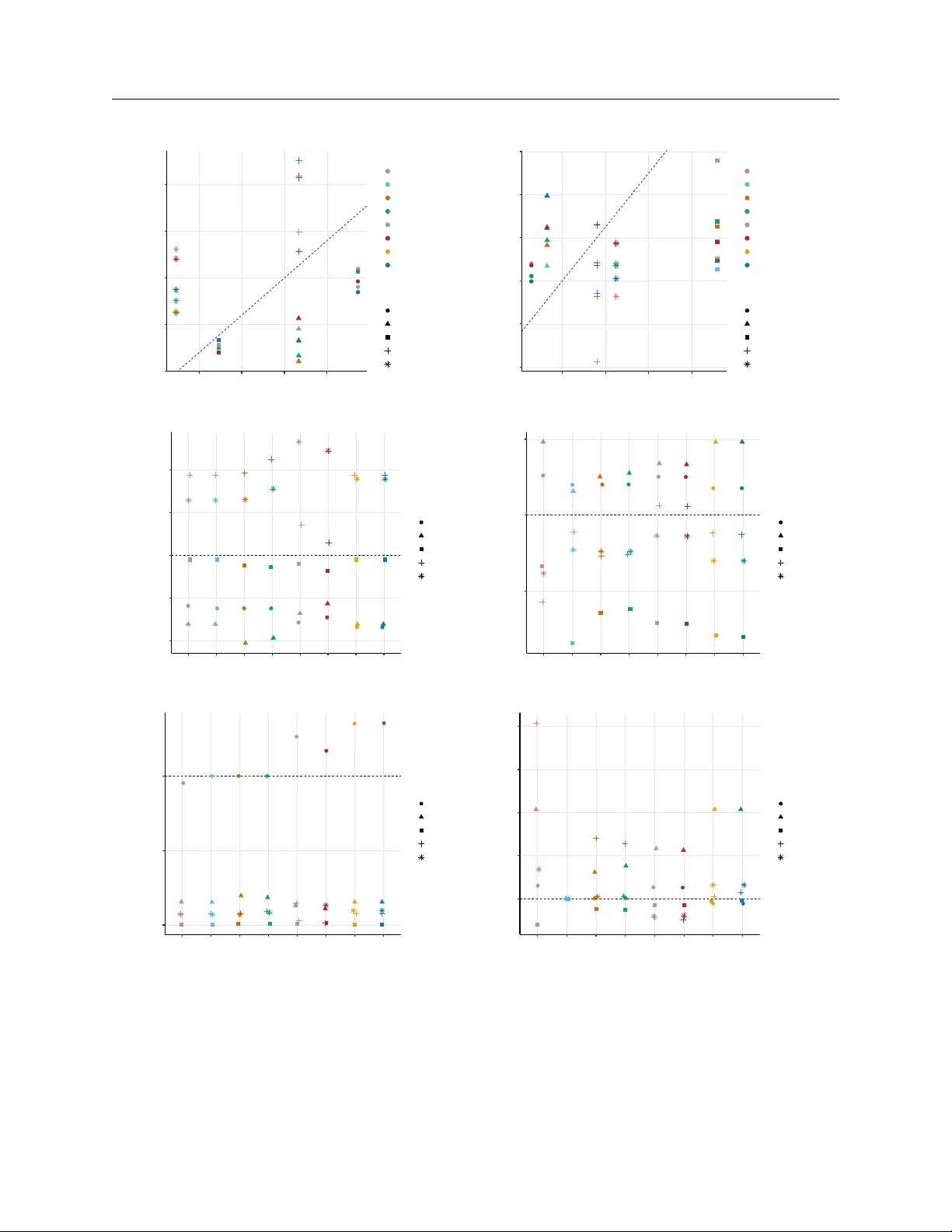
Detecting and Mitigating Group Bias in Heterogeneous T reatmen t Eﬀects Jo el P ersson* † Spotify Jurri ¨ en Bakk er Booking.com Dennis Bohle Booking.com Stefan F euerriegel Munich Center for Machine Learning & LMU Munich Florian v on W angenheim ETH Zurich Heterogeneous treatment eﬀects (HTEs) are increasingly estimated using machine learning mo dels that pro- duce highly p ersonalized predictions of treatmen t eﬀects. In practice, ho wev er, predicted treatmen t eﬀects are rarely interpreted, rep orted, or audited at the individual lev el but, instead, are often aggregated to broader subgroups, suc h as demographic segments, risk strata, or mark ets. W e show that suc h aggregation can induce systematic bias of the group-lev el causal eﬀect: even when models for predicting the individual-level conditional a verage treatment eﬀect (CA TE) are correctly speciﬁed and trained on data from randomized exp erimen ts, aggregating the predicted CA TEs up to the group level do es not , in general, recov er the corre- sp onding group a verage treatment eﬀect (GA TE). W e develop a uniﬁed statistical framew ork to detect and mitigate this form of group bias in randomized exp erimen ts. W e ﬁrst deﬁne group bias as the discrepancy b et w een the mo del-implied and exp erimen tally identiﬁed GA TEs, derive an asymptotically normal estima- tor, and then pro vide a simple-to-implement statistical test. F or mitigation, we prop ose a shrink age-based bias-correction, and show that the theoretically optimal and empirically feasible solutions hav e closed-form expressions. The framew ork is fully general, imp oses minimal assumptions, and only requires computing sam- ple moments. W e analyze the economic implications of mitigating detected group bias for proﬁt-maximizing p ersonalized targeting, thereby characterizing when bias correction alters targeting decisions and proﬁts, and the trade-oﬀs inv olved. Applications to large-scale exp erimen tal data at ma jor digital platforms v alidate our theoretical results and demonstrate empirical performance. Key wor ds : heterogeneous treatment eﬀects; causal mac hine learning; bias detection; bias mitigation; randomized exp eriments ∗ This research w as initiated during the author’s PhD at ETH Zurich. It w as completed indep endently of the author’s curren t emplo yment at Sp otify . † Corresp onding author, email: joelp ersson@sp otify .com 1 2 1. In tro duction Heterogeneous treatment eﬀects (HTEs)—the presence of systematic v ariation in treatment eﬀects across individuals or subgroups—hav e b ecome central to how organizations learn ab out and target in terv en tions across a wide range of domains, including mark eting (e.g., Lemmens et al. 2025, Hitsc h et al. 2024) and healthcare (e.g., F euerriegel et al. 2024, Kraus et al. 2024). Recen tly dev elop ed metho ds based on mac hine learning (ML) (e.g., A they and Im b ens 2016, W ager and A they 2018, Chernozh uk o v et al. 2018a) ha v e made it p ossible to estimate highly p ersonalized HTEs by mo deling conditional a verage treatment eﬀects (CA TEs) as ﬂexible functions of ric h, high-dimensional, and individual-lev el co v ariates. While individualized CA TE predictions ha ve been adopted for automated decision-making related to p ersonalization (Lemmens et al. 2025), treatment eﬀect estimates themselves are typi- cally not interpreted, rep orted, or audited at the individual level. Instead, they are aggr e gate d to subgroups of substantiv e in terest to the business, organization, or research question at hand, such as demographic segmen ts, risk strata, or mark ets. This practice reﬂects b oth an interest in more generalizable subgroup-lev el eﬀects and the fact that ML-based CA TEs are functions. F or instance, digital platforms may p ersonalize recommendations to individual users while inferring eﬀects at the segment lev el (Lemmens et al. 2025); medical professionals may deploy individualized treat- men t rules while ev aluating eﬀects b y clinically relev an t strata (suc h as young vs. old or smokers vs. non-smokers) (Hernan and Robins 2023); and ﬁrms and lab or market programs may use ML systems for p ersonalization while rep orting outcomes for coarser groups deﬁned b y age, lo cation, or other characteristics (Agraw al et al. 2025, A they and Palik ot 2022). More generally , whenever CA TE estimates are plotted, tabulated, or summarized ov er bins or discrete cov ariates, they are implicitly b eing summarized to treatmen t eﬀects for groups. Despite this widespread practice, it is less recognized that suc h subgroup-level summaries, in general, do not recov er a causal eﬀect. F or this to hold, the appropriately w eighted group-av erage of the CA TE must equal the estimand of the corresp onding group-a v erage treatmen t eﬀect (GA TE). This is a strong requiremen t and ma y fail ev en when the CA TE is point-iden tiﬁed, correctly spec- iﬁed, and un biased and consisten tly estimated. As a result, subgroup-level aggregates of CA TEs learned even under ideal conditions ma y lac k a causal in terpretation. More generally , this problem reﬂects the distinction b etw een unbiasedness, confounding, and collapsibilit y in causal inference (Greenland et al. 1999, Huitfeldt et al. 2019, Didelez and Stensrud 2022, Colnet et al. 2023). 1 In this paper, we study the problem of detecting and mitigating this group bias in personalized CA TE predictions from experimental data. Using a st ylized example (Section 3), we ﬁrst show that even state-of-the-art CA TE learners trained on exp erimental data can exhibit systematic group bias relative to the corresp onding GA TE. Perhaps surprisingly , including group indicators, estimating separate CA TE mo dels p er group, or using more training data, do es not necessarily remo v e the group bias and may even b e practically infeasible. In many settings, groups of interest 1 Collapsibilit y refers to the prop erty that a conditional eﬀect measure, when prop erly marginalized, recov ers the corresp onding marginal eﬀect measure. An estimator may b e unbiased and unconfounded yet not collapsible (see, e.g., Greenland et al. 1999). 3 are deﬁned ex p ost by diﬀerent stakeholders, such as, managers, researc hers, or auditors, and is often una v ailable at training time due to priv acy , legal, or op erational constraints. 2 Another k ey c hallenge of the problem is that only randomized exp erimen ts pro vide reliable b enchmarks for mo del-implied estimates, yet they cannot pro duce evidence of treatment eﬀects at the same level of gran ularit y as CA TEs from ML. Because p otential outcomes are nev er jointly observ ed (Holland 1986) and p ersonalized CA TE estimates condition on man y individual-level cov ariates, mo del-free exp erimen tal estimators suc h as diﬀerence-in-means can only b e applied at more aggregate lev els, suc h as those that iden tify GA TEs. Thus, rather than measuring or correcting bias at the individual lev el, we aim to reliably detect and mitigate bias in CA TE predictions at the group lev el—for whic h exp erimen ts pro vide nonparametric iden tiﬁcation and mo del-free estimation. W e aim to mak e three con tributions: First , w e in tro duce a general metho dology for detecting group bias in CA TE predictions from randomized experiments (Section 4). W e deﬁne group bias as a causal estimand capturing the discrepancy b et ween model-implied and exp erimentally iden tiﬁed GA TEs, that is, whether aggre- gating predicted CA TEs recov ers the corresp onding subgroup treatment eﬀects. W e introduce a general, asymptotically normal estimator of this group bias and pro vide a formal statistical test for detection. The resulting pro cedure is nonparametric, mo del-agnostic, and applies to b oth binary and con tin uous outcomes, diﬀerent scales of treatmen t eﬀects (i.e., additive and relativ e eﬀect scales), and arbitrary CA TE learners under minimal assumptions. Se c ond , w e propose a shrink age-based bias-correction approach for mitigation. A na ¨ ıv e correction b y simply subtracting the estimated bias p er group, akin to standard bias-correction, remov es group bias only in exp ectation. In ﬁnite samples, this may incr e ase the disp ersion of group bias among the groups, as it tends to ov ercorrect for smaller or noisier groups. As a solution, we formulate mitigation as choosing how muc h to debias (i.e., how muc h to shrink the correction) in order to minimize the exp ected loss (risk) of residual group bias. F or natural loss functions, w e derive the closed-form oracle minimizer as well as feasible estimators, b oth of whic h automatically adjust the debiasing to the signal-to-noise ratio of the estimated group bias. W e apply our framework to large- scale A/B test data from a leading online trav el platform to demonstrate empirical p erformance and v alidate our theoretical results (Sections 5 and 6). Thir d , we analyze the implications of mitigating detected group bias in p ersonalized CA TE predictions for decision-making. By fo cusing on proﬁt-maximizing p ersonalized targeting, we char- acterize ho w bias correction alters the optimal decision rule, targeting decisions, and expected proﬁts, and the factors that contribute to this (Section 6). W e illustrate our theoretical insights using counterfactual oﬀ-p olicy ev aluation on the Criteo Uplift Prediction Dataset (Diemert et al. 2 Ev en if group indicators are included, they can b e dropp ed by regularization, eﬀectively limiting the group-wise heterogeneit y in treatment eﬀects captured by the mo del. Moreov er, re-training the mo del separately within each group amoun ts to re-estimating a nonparametric treatmen t response function at smaller and potentially noiser subsets of the data, thus requiring even stronger assumptions than for the original mo del that is presumed to b e biased (such as suﬃcient ov erlap within each group), and may therefore introduce new forms of bias. Assuming regularization do es not drop the indicators and that the stronger within-group iden tiﬁcation conditions are met, estimation is still sub ject to diﬀeren tial sample sizes and signal-to-noise across groups, whic h may still in tro duce group bias. 4 2018). W e then discuss the resulting trade-oﬀs and provide practical guidance for implementation (Section 7). 2. Related W ork Our study connects to three strands of researc h: (1) algorithmic bias in mac hine learning, (2) bias in causal inference, and (3) bias mitigation and its implications. 2.1. Algorithmic Bias in Machine Learning Our work is related to, but distinct from, the literature on algorithmic bias and algorithmic fairness. In that literature, bias is t ypically op erationalized as a prediction or decision problem: bias is said to exist if there are systematic disparities in predictive accuracy , error rates, or decision outcomes across groups deﬁned by protected attributes (Chouldec ho v a and Roth 2020, Baro cas et al. 2023, Castelnov o et al. 2022, Corb ett-Davies et al. 2017, De-Arteaga et al. 2022). Related w ork on algorithmic fairness, often motiv ated by legal or ethical considerations, studies how such disparities should b e mitigated, typically b y mo difying prediction mo dels or downstream decision rules (Kleinberg et al. 2018). Diﬀeren t from this literature, we do not study bias in individual- lev el C A TE predictions or downstream decisions p er se, but bias that arises when p ersonalized treatmen t eﬀect predictions are aggregated to reco v er group-lev el causal estimands. While causal or coun terfactual notions are sometimes used to deﬁne measures of bias or fairness (see, e.g., Carey and W u 2022, Nilforoshan et al. 2022), the ob ject being predicted is typically not itself a causal eﬀect, and the causal estimand obtained after mitigation is often left implicit. Our w ork diﬀers in that w e fo cus on causal inference, with b oth the individual-lev el prediction, the group-lev el estimand, and the bias obtained once aggregating the former to the latter, all relate to treatmen t eﬀects. Metho dologically , several pap ers in the algorithmic bias literature frame bias detection as a sta- tistical testing problem, fo cusing on bias in outcome predictions or classiﬁcation decisions (T askesen et al. 2021, DiCiccio et al. 2020, Yik et al. 2022). Although w e also employ statistical testing, the bias we study is fundamentally diﬀerent. Because individual-level treatmen t eﬀects are unobserved (Holland 1986), bias assessment for CA TE mo dels necessarily pro ceeds through aggregation. 3 In the lens of this literature, our con tribution is thus to show that ML mo dels of p ersonalized CA TEs will tend to b e biased when summarizing the CA TES into the causal eﬀects at broader groups of in trinsic in terest. 2.2. Bias in Causal Inference Our work also connects to researc h on bias in causal inference. Here, we distinguish three diﬀeren t issues: bias from identiﬁcation failures, calibration, and bias from am biguity in the causal estimand. 3 Here, we refer to settings in which the CA TE mo del dep ends on many and/or con tinuous cov ariates, as this is precisely the regime that motiv ates ML-based estimation for p ersonalization. T o assess bias in such settings, training a new CA TE mo del is not a viable solution, as the original mo del is presumed to b e biased, and mo del-free estimates from experiments, such as diﬀerence-in-means, identify treatment eﬀects only at more aggregate levels. 5 First, Gordon et al. (2019, 2023) show that ML estimators for causal inference often fail to reco v er experimental estimates of a verage treatment eﬀects, essen tially revisiting the LaLonde critique (LaLonde 1986) with modern methods (Im b ens and Xu 2024) and marketing data. In these w orks, the discrepancy reﬂects an identiﬁc ation pr oblem : observ ational data do not supp ort the assumptions required to recov er the target estimand. Our work highligh ts a diﬀerent issue. Even when CA TE mo dels are correctly identiﬁed, speciﬁed, and estimated, aggregating their predictions can fail to recov er in tended subgroup-level treatment eﬀects. This can arise b ecause mo dels are trained to optimize global rather than group-sp eciﬁc ob jectives, or b ecause regularization shrinks mo deled heterogeneit y (Chernozh uk o v et al. 2018a, Meln yc h uk et al. 2024). Our work is also related to metho ds that summarize or ev aluate estimated CA TEs, but diﬀers in b oth aims and approach. Chernozhuk o v et al. (2018b) aim to summarize the predictiv e conten t of CA TE for more aggregate groups. They do so b y sorting predicted CA TES in to bins and then using regressions to p erform inference on the av erage CA TE p er bin. Leng and Dimmery (2024) aim at calibrating CA TE across its distribution, by regressing the a v erage CA TE within calibration bins on to exp erimen tal subgroup eﬀects. In these works, “groups” are technical devices endogenously deﬁned b y quantiles of the CA TE distribution. In con trast, in our work, groups are deﬁned by a manager, p olicy-mak er, or researc her (e.g., mark ets, segmen ts, or demographic attributes), and the question is whether aggregating individual-lev el CA TE predictions within groups recov ers the group-lev el causal eﬀect, and ho w to correct for the potential bias. As such, our w ork is motiv ated b y a practical use of CA TE mo dels, rather than by their prop erties. Moreov er, while those work fo cuses on additiv e eﬀect measures, our framework also applies to relative treatmen t eﬀects, suc h as relativ e risk and lift factors, commonly used in health sciences and mark eting. In doing so, our researc h connects to recen t econometric literature highligh ting when commonly used estimation practices fail to recov er the causal estimands researchers in tend to estimate (e.g., Go o dman-Bacon 2021, Goldsmith-Pinkham et al. 2024). Among these w orks, the issue is that the a v erage treatment eﬀect is not identiﬁed b y the estimation strategy in question when individual- lev el eﬀects are heterogeneous. This issue is related to the concept of c ol lapsibility from the causal inference literature, whic h c haracterizes when p opulation-marginal causal eﬀects (suc h as the A TE) can b e recov ered from weigh ted av erages of conditional eﬀects (Huitfeldt et al. 2019, Didelez and Stensrud 2022, Colnet et al. 2023). W e extend this logic from p opulation-level eﬀects to subgroup- lev el eﬀects, showing when aggregation of individual-level CA TEs fails to recov er group-av erage treatmen t eﬀects (GA TEs), and prop ose metho ds to detect and mitigate the resulting group bias. 2.3. Bias Mitigation and Its Implications Finally , our work relates to research on bias mitigation and its implications. One line of work in mark eting studies bias in ML mo dels for CA TE sp eciﬁcally . Ascarza and Israeli (2022) introduce fairness constraints in the training of causal trees to regulate downstream targeting across groups, while Huang and Ascarza (2023) prop ose how to calibrate aw ay bias in CA TE estimates induced b y priv acy-preserving noise in the training data. While b oth papers fo cus on personalized CA TEs, they target diﬀeren t bias ob jects and are tied to sp eciﬁc learners, constraints, or data-generating 6 pro cesses. By contrast, w e fo cus on errors that arise when aggr e gating CA TE into group-lev el treatmen t eﬀects, while remaining agnostic to the mo del. Another stream of research studies the consequences of constraining how predictiv e mo dels are used. Ram bachan et al. (2020) dev elop an economic model of how group-level constraints on predic- tiv e allocations aﬀect optimal decision rules in hiring, while related w ork examines applications in business analytics (De-Arteaga et al. 2022) and public p olicy (Corb ett-Davies et al. 2017, Chohlas- W o o d et al. 2023). A recurring insight in this literature is that correcting group-level disparities in individual-level predictions do es not necessarily yield the in tended economic or allo cative out- comes. F or example, De-Arteaga et al. (2022) pro vide coun terp oints to the personalization–fairness “trade-oﬀ ”, while Chohlas-W o o d et al. (2023) sho w that allo cation rules designed to promote equity can b e P areto-dominated b y purely eﬃciency-orien ted p olicies. Our analysis of targeting implications is conceptually related but diﬀers in fo cus. Rather than studying fairness or equit y , we examine the trade-oﬀ that arises when personalized treatment eﬀect predictions are used b oth for aggregate causal inference and for individualized treatment decision- making. In this setting, correcting aggregated CA TE predictions to reco ver GA TEs impro ves group- lev el causal inference but can alter targeting decisions, resulting in proﬁt loss relativ e to using the ra w CA TE predictions. Our analysis clariﬁes when such trade-oﬀs arise and ho w they dep end on the chosen bias-mitigation strategy . W e distill these insights into practical guidance for how managers and ﬁrms can na vigate this trade-oﬀ, helping to rationalize wh y coarser targeting policies ma y b e preferred ev en when more granular p ersonalization is technically feasible (Lemmens et al. 2025). 3. Motiv ating Example T o build intuition for why group bias can arise in ML mo dels of heterogeneous treatmen t eﬀects, w e consider a motiv ating example in which a p ersonalized CA TE mo del is trained on exp erimental data and then ev aluated b y aggregating predictions to ex post-deﬁned groups. The example shows that systematic group bias can arise even under correct identiﬁcation and speciﬁcation, and is not sp eciﬁc to an y particular estimation approac h. The same logic extends to multiple groups and, as sho wn later, to relativ e eﬀect measures. Supp ose we observe data on N individuals indexed by i = 1 , . . . , N . F or each individual, let X i denote a vector of pre-treatment cov ariates, T i ∈ { 0 , 1 } a binary treatment assigned uniformly at random, and let p oten tial outcomes b e giv en b y Y i (0) = µ 0 ( X i ) + ε i 0 , Y i (1) = µ 1 ( X i ) + ε i 1 , (1) where µ t ( x ) = E [ Y ( t ) | X = x ] and the errors ε i 0 , ε i 1 ha v e mean zero and ﬁnite v ariance. The CA TE is τ ( x ) = µ 1 ( x ) − µ 0 ( x ) , (2) whic h we assume is a smooth, learnable function of X . In this data-generating pro cess, the standard iden tiﬁcation assumptions hold: There is no in terference betw een units (stable unit treatmen t v alue 7 assumption), and the treatment is randomly assigned, implying no confounding and o verlap. As a result, τ ( x ) is p oint-iden tiﬁed, and w e can use a mo del f to obtain a CA TE estimate b τ f ( x ) from the data ( X i , T i , Y i ) N i =1 . One w ay to represent this estimation task is empirical risk minimization, where the ob jectiv e is to solv e min τ E h  Y − µ 0 ( X ) − T · τ ( X )  2 i , (3) with ﬁnite-sample analogs implemented via meta-learners (K ¨ unzel et al. 2019), causal forests (W ager and Athey 2018, Athey et al. 2019), and related metho ds. Another representation is esti- mating equations: mo dern causal ML estimators solv e momen t conditions of the form E  ψ ( { X , T , Y } ; τ , η 0 )  = 0 , (4) for some estimating function ψ ( · ), p ossibly after orthogonalization with respect to nuisance param- eters η 0 (Chernozh uk o v et al. 2018a). This encompasses double/debiased ML, doubly robust (DR) learners (Kennedy 2023), R-loss minimization (Nie and W ager 2021), and other orthogonal learners (F oster and Syrgk anis 2023). In all cases, the CA TE mo del is trained to optimize an ob jective o v er the data, under regularization and h yp erparameter tuning to con trol mo del complexit y . No w supp ose that, after the CA TE mo del has b een trained, a binary group v ariable G ∈ { 1 , 2 } is introduced to analyze the data at diﬀerent segmen ts of managerial, organizational, or research relev ance. Essentially , the v ariable G partitions the p opulation into tw o groups of unequal size, with N 1 > N 2 . The group indicator may b e included among the co v ariates X or correlated with them, but it do es not aﬀect treatmen t assignmen t per its randomization. The induced groups ma y therefore diﬀer arbitrarily in their cov ariate distributions and outcome distributions, even though treatmen t remains randomized within eac h group. Our interest lies in using the trained CA TE mo del to infer GA TEs τ g = E [ τ ( X ) | G = g ], g ∈ { 1 , 2 } by aggr e gating the individual-lev el CA TE predictions via subgroup sample a v erages, b τ f g = E N [ b τ f ( X ) | G = g ]. W e illustrate the resulting tension using a simple sim ulation. W e set sample sizes to N 1 = 150 and N 2 = 100, generate T i ∼ Bernoulli(1 / 2), and draw tw o contin uous cov ariates from group-sp eciﬁc biv ariate normal distributions. 4 The true CA TE τ ( X ) is constructed as a nonlinear function of the co v ariates with diﬀeren t group means, and thus generating diﬀerent GA TEs τ g . Outcomes are generated as Y i = Y i (0) + T i τ ( X i ). W e then construct a generic CA TE predictor b y p erturbing the true CA TE with group-sp eciﬁc mean shifts and mean-zero noise, chosen so that the predictor is un biased in the p opulation but systematically biased within groups. W e also estimate CA TEs using a range of representati ve and widely used causal ML mo dels, namely , causal forests, metalearners (S-, T-, and X-learners), and the DR-learner, which w e implemented using the grf , glmnet , and randomForest pack ages in R with default h yp erparameter v alues. 5 W e include the group indicator 4 The sample sizes are c hosen for visual clarit y; increasing them narro ws the precision of the group bias of CA TE in GA TE without changing its sign or magnitude. 5 W e implement causal forests using grf , the metalearners with random forests for the outcome regressions, and the DR-learner via 5-fold cross-ﬁtted estimation of the propensity score and outcome regressions using regularized 8 Figure 1 Simulation illustration of group bias in CA TE predictions. 0.0 0.2 0.4 0.6 0.8 0.0 0.2 0.4 0.6 0.8 Predicted CA TE T r ue CA TE Group 1 (large) Group 2 (small) 0.0 0.2 0.4 0.6 0.8 GA TE Group 1 Group 2 Predicted T r ue 0.0 0.2 0.4 0.6 0.8 GA TE Group 1 Group 2 T r ue Causal Forest T−Learner S−Learner X−Learner DR−Learner Note. (L eft) : A generic CA TE mo del, given b y the true CA TE plus errors with group=wise heteroskedastic v ariance, o verestimates CA TE for the larger group ( N = 150) and underestimates CA TE for the smaller group ( N = 100). The dashed 45 ° line signiﬁes no estimation errors. (Center) : Av eraging the CA TE predictions p er group yields GA TEs that diﬀer in bias. (Right) : Causal ML estimates of CA TE are also biased of GA TE, despite satisfying all iden tiﬁcation assumptions, b eing correctly sp eciﬁed, and trained on data with with randomized treatment. Error bars are 95% conﬁdence interv als based on normal approximation. G i when training the mo dels to allow them to capture the group-wise heterogeneity . All mo dels then satisfy p oin t-iden tiﬁcation, and are correctly sp eciﬁed. Figure 1 summarizes the results. In the left panel, the generic CA TE predictions are centered around the 45-degree line, indicating no ov erall bias. How ev er, conditional on group membership, predictions systematically understate treatment eﬀects for the larger group and o verstate them for the smaller group. When these predictions are aggregated to the group lev el, the resulting GA TE estimates diﬀer systematically from the true GA TEs (center panel). The bias is statistically signiﬁcan t at the 5% level for b oth groups, and the sign and magnitude v ary . The same qualitative pattern app ears for the causal ML estimators (right panel), with the sign and magnitude of the group bias now also v arying across mo dels. This demonstrates that even under ideal identiﬁcation and correct speciﬁcation, ML mo dels that are un biased for individual-lev el CA TE can exhibit systematic and uncon trolled bias of group-lev el eﬀects. 6 4. F ramew ork This section provides our framew ork. W e ﬁrst in tro duce the relev ant estimands and then presen ting metho ds and theory for the detection and mitigation of group bias from exp erimen tal data. generalized linear mo dels ( glmnet ), follow ed by a second-stage regression of the resulting orthogonalized (AIPW) pseudo-outcome on cov ariates using a random forest. 6 An underlying mechanism is that the mo dels are trained to optimize global ﬁt ov er the full distribution of the data, whether by empirical risk minimization, solving a momen t condition, or some orthogonalized v ersion thereof (as in Chernozh uko v et al. 2018a, F oster and Syrgk anis 2023, Nie and W ager 2021). Under regularization and heterogeneous group sizes, cov ariate distributions, and signal-to-noise ratios, prediction errors then need not cancel symmetrically within the groups c hosen ex post. 9 4.1. T reatmen t Eﬀect Estimands W e consider individual-lev el exp erimental data on pre-treatment co v ariates X , a randomly assigned treatmen t T ∈ { 0 , 1 } , and an outcome Y that may b e binary or con tin uous. The random v ariables ( X , T , Y ) are drawn i.i.d. from a distribution P . The data are partitioned into groups indexed b y G ∈ G , where G may b e contained in X . Groups ma y represent demographic attributes, market segmen ts, or some other one-dimensional partitioning of in terest, or they may b e deﬁned as a function of observed v ariables. 7 F or each group g ∈ G , let P g denote the conditional distribution of ( X , T , Y ) giv en G = g , which ma y diﬀer arbitrarily across groups. In a sample of size N = P g ∈G N g from P , group sizes N g ma y also v ary . There is a pre-existing ML mo del f : X 7→ b τ f ( X ), where b τ f ( X ) is its prediction of the (true) CA TE, deﬁned on an additiv e or relativ e scale as τ ( X ) = E [ Y (1) − Y (0) | X ] and τ ( X ) = E [ Y (1) | X ] E [ Y (0) | X ] , (5) resp ectiv ely . The mo del was trained on some prior data using a p ossibly unknown ob jective and pro cedure. No assumptions are imp osed on it b ey ond standard regularity conditions, such as that its predictions hav e ﬁnite v ariance, and that w e can obtain its CA TE prediction for eac h observ ation. W e are in terested in whether the mo del’s CA TE predictions reco v er the GA TE, deﬁned as τ g = E [ Y (1) − Y (0) | G = g ] and τ g = E [ Y (1) | G = g ] E [ Y (0) | G = g ] , (6) resp ectiv ely . Either estimand τ g can b e estimated from the treated and con trols observ ations p er group, also via appropriate regression adjustmen t estimators (see App endix B for details). Additiv e eﬀects for contin uous outcomes are standard in the statistics and econometrics liter- ature based on the p otential outcomes framew ork. They directly answer questions such as the dollar impact of a promotion on sales or the eﬀect of a medical treatmen t on blo o d pressure. In applied research and practice, how ever, relative eﬀects are also widely used due to their scale-free, p ercen tage-c hange interpretation and are commonly used when binary outcomes are of primary in terest. 8 F or example, in the health sciences, interest often lies in eﬀects on adverse ev ents suc h as disease onset or death, while in mark eting and the tec h sector, common binary outcome is conv er- sion. In these settings, E [ Y ( t )] = Pr( Y ( t ) = 1), and so the treatmen t eﬀect estimands corresp ond to a causal measure of the risk diﬀerence and relative risk, whic h are standard in the health sciences (Greenland et al. 1999, Hern´ an and Robins 2006), or magnitude and relativ e measures for “lift”, whic h are standard in adv ertising measurement and incrementalit y testing (see e.g., the measures in Section 4.1. and 5.2 in Gordon et al. 2023). It is worth noting that, although additiv e and relative 7 Groups may also be deﬁned or data-driven manner, provided they are deﬁned independently of the bias detection and mitigation pro cedures. Examples of the latter include quan tiles of predicted outcomes (risk or c h urn quan tiles), or clusters constructed using pre-treatment information 8 F or relative eﬀects to b e well-deﬁned, denominators must b e strictly p ositive. A common ad-ho c ﬁx is to add a small constant to the numerator and denominator, analogous to practices for ﬁtting regression mo dels with zero- v alued log-transformed outcomes. How ever, this can introduce bias. More principled approaches include modeling on appropriate scales (e.g., via log-link GLMs). 10 eﬀects are expressed on diﬀerent scales, they are equiv alen t via simple transformations: relativ e eﬀects are additive eﬀects scaled b y the mean baseline p otential outcome or, equiv alently , they are additiv e eﬀects measured on the log scale and then transformed bac k. 9 Our framew ork applies to b oth additiv e and relative eﬀect measures. The distinction matters b ecause aggregation from CA TEs to GA TEs b ehav es diﬀerently across the scales, as we show in the next section. 4.2. Group Bias T o formalize group bias of CA TE predictions relativ e to GA TEs, we ﬁrst distinguish b etw een tw o sources: estimation error in the CA TE itself and bias induced b y aggregation. This distinction is crucial, as only the former represen ts the underlying CA TE error of interest, while the latter m ust b e con trolled to ensure that such errors propagate into an error in the GA TE rather than an ill-deﬁned or misaligned estimand. Separating the tw o allows detected group bias to b e interpreted as error in the GA TE and ensures that statistical inference targets precisely this ob ject. W e b egin by contrasting what holds at the p opulation level with what o ccurs in ﬁnite samples for a given group. When treatment eﬀects are deﬁned on the additive scale, the p opulation A TE satisﬁes E [ Y (1) − Y (0)] = E X { E [ Y (1) − Y (0) | X ] } = E X [ τ ( X )] . (7) This equality explains why most ML mo dels of the A TE ﬁrst estimate τ ( X ) and then av erages them o v er the cov ariate distribution used for training. In ﬁnite samples, es timation errors in CA TE tend to cancel symmetrically when a v eraged ov er the same distribution, yielding an accurate estimate of the A TE. Ho w ev er, this aggregation prop ert y does not generally hold o ver arbitrary subgroups. The reason is not a failure of identiﬁcation, but of estimation combined with aggregation: CA TE is either esti- mated via a single model trained to minimize error o ver the p opulation, or separately for subgroups that v ary in size and distribution. Then, estimation errors need not cancel within groups, nor b e equal in magnitude across groups. This issue is exacerbated by that causal ML mo dels typically rely on asymptotic guarantees and regularization, which can penalize heterogeneity unev enly when sample sizes or signal-to-noise ratios diﬀer. When treatment eﬀects are instead measured on a relative scale via ratios, an additional com- plication is in tro duced. Because ratios aggregate nonlinearly , the exp ectation of relativ e CA TEs generally do es not p oint-iden tify the corresp onding group-lev el estimand. By Jensen’s inequality , w e ha v e E [ τ ( X )] = E  E [ Y (1) | X ] E [ Y (0) | X ]  ≥ E { E [ Y (1) | X ] } E { E [ Y (0) | X ] } = τ . (8) Hence, the simple av erage of relative CA TEs recov ers an estimand that is not a GA TE but instead (w eakly) upw ard biased relative to it. Because Eq. (8) is deriv ed with resp ect to the true CA TE, this issue arises ev en when τ ( X ) is kno wn or estimated p erfectly . 9 An y ratio E [ Y (1)] / E [ Y (0)] can b e written as E [ Y (1) − Y (0)] / E [ Y (0)] + 1 or equiv alently as exp(log E [ Y (1)] − log E [ Y (0)]). 11 T o address bias from aggregation, and ensure group-level errors reﬂects the CA TE mo del itself, w e dra w on the concept of c ol lapsibility (Colnet et al. 2023). Definition 1 (Collapsibility). L et P { X , Y (0) } denote the joint distribution of c ovariates and b aseline p otential outc omes. A tr e atment eﬀe ct me asur e τ is collapsible if ther e exists a weight function W = w ( X , P ( X , Y (0))) such that E P [ W τ ( X )] = τ , W ≥ 0 , E P [ W ] = 1 . (9) Collapsibilit y formalizes when a conditional treatment eﬀect estimand can b e aggregated to its marginal estimand. It is a prop ert y of the estimand and not just of its estimate. Additiv e eﬀects are collapsible with uniform weigh ts ( W = 1), recov ering the familiar linear aggregation result men tioned earlier. F or relative eﬀects, the appropriate weigh ts are W ( X ) = E [ Y (0) | X ] / E [ Y (0)] (Greenland et al. 1999, Colnet et al. 2023), reﬂecting that the marginal relativ e eﬀect is a ratio of means rather than a mean of ratios (cf. Eq. (8)), and therefore requires w eigh ting conditional ratios b y their baseline p oten tial outcomes. 10 W e can no w deﬁne a causal estimand of group bias in CA TE. Definition 2 (Group Bias). L et b τ f ( X ) b e a pr e diction of τ ( X ) fr om a mo del f , and let W b e a weight function satisfying Def. 1 within gr oup g ∈ G . We deﬁne the group bias of the mo del as b g = E P g  W ( b τ f ( X ) − τ ( X ))  . (10) The expression mirrors the canonical deﬁnition of bias in statistics, but conditional on a group and appropriately weigh ted so error in CA TE propagates to bias with resp ect to the causal estimand of GA TE. As sho wn in Section 3, the group bias will generally diﬀer across groups. T o assess whether bias is unev enly distributed, one can consider contrasts in the group bias. A natural measure is the cr oss- gr oup bias b g − b − g , where b − g = P k ∈G \ g b k Pr[ G = k ] is the av erage bias across all other groups. This estimand captures whether the bias induced b y a CA TE mo del for group g diﬀers systematically from that of the remaining p opulation, and pro vides a basis for across-group comparisons. 11 Tw o examples illustrate wh y detecting and mitigating the group bias can matter in practice. Example 1. Supp ose a ﬁrm ﬁts a CA TE mo del on its customer data and then wan ts to target promotional oﬀers tow ards segments that diﬀer in size and demand elasticity . One segment has particularly strong demand elasticity—for example, due to low er a v erage income or higher price sensitivit y—but is made up of c omparativ ely few customers. Aggregating the customer-lev el CA TE predictions to segment-lev el GA TEs would then tend to underestimate the GA TE for this high- resp onse segment. If the ﬁrm has a budget constrain t on the num b er of promotions or thresholds the GA TEs to decide which segmen t to target, then this segment w ould receiv e fewer promotions than in optimum, and total targeting proﬁts and customer surplus would b e low er than attainable. 10 Not all eﬀect estimands are collapsible; e.g., conditional (log) o dds ratios are not. 11 One may also consider pairwise contrasts b g − b h for any h  = g in G , scalar disp ersion measures such as V ar G [ b B g ] for estimates ( b B g ), or empirical densities ov er ( b B g ). W e later provide results based on the latter tw o (cf. App endix E to the empirical results in Section 5.4 and Appendix D on a sim ulation study . 12 Example 2. Supp ose a public health agency w ants to promote COVID-19 v accination for demo- graphic groups according to their COVID risk. T o do so, the agency conducts large-scale random- ized con trolled trial to learn the CA TE of individual v accine resp onse, which can then inform an outreac h targeting p olicy . Consider that African Americans w ere underrepresented in such trials despite facing ab ov e-av erage relative risk from CO VID (W arren et al. 2020, Artiga et al. 2020). Their estimated risk by the mo del-implied GA TE would then b e down w ard biased tow ards the p opulation-marginal A TE, potentially causing ineﬃcien t targeting b y the public health agency and sub optimal health outcomes for this high-risk group. 4.3. Detection 4.3.1. Estimation via Decomp osition of Group Bias. W e no w describ e a general approac h for estimating and detecting group bias in CA TE predictions. The main idea is that, although the CA TE τ ( X ) is unobserv able, the group bias of a CA TE mo del can be decomposed as simply the diﬀerence b et w een t w o group-lev el aggregates that are directly estimable: b g = E P g  W b τ f ( X )  − E P g [ W τ ( X ) ] = τ f g |{z} model-implied GA TE − τ g |{z} true GA TE , (11) where the ﬁrst equality follows b y applying linearit y of exp ectations to Eq. (10) and the second b y Deﬁnition 1. Here, τ f g = E P g [ W b τ f ( X )] is the p otentially-biased GA TE parameter implied by the CA TE mo del using the true weigh ts, and τ g is the corresp onding GA TE estimand deﬁned in Eq. (6). This decomp osition holds for an y model of CA TE used and irrespective of whether eﬀects are deﬁned as diﬀerences or ratios. Therefore, a general estimator can b e written as b B g = b τ f g − b τ g , (12) where b τ f g = E N g [ c W b τ f ( X )], and c W are estimates of the weigh ts W = E [ Y (0) | X , G ] / E [ Y (0) | G ] if eﬀects are measured on a relativ e scale (cf. the discussion after Deﬁnition 2) and c W = 1 if not, and b τ g is an estimate of GA TE for the same group. Hence, estimating the group bias in CA TE do es not require the actual CA TE: it suﬃces to compare prop erly aggregated predictions to a direct estimate of GA TE. In randomized exp eriments, the weigh ts required to collapse ratio CA TEs are nonparametrically iden tiﬁed and easily estimated. In particular, randomization implies that E [ Y (0) | X, G ] / E [ Y (0) | G ] is iden tiﬁed b y E [ Y | X , G, T = 0] / E [ Y | G, T = 0], whic h can b e estimated by ﬁtting regression mo d- els to the non-treated using a group indicator and cov ariates as controls, and then taking the ratio of ﬁtted v alues p er observ ation. 12 The estimated GA TE b τ g , in turn, is obtained via the appropriate con trast-in-means (diﬀerence or ratio) or regression-adjustmen t estimator; see App endix B. 13 12 It is useful to consider when w eighting for collapsing ratio CA TEs is necessary . Because the weigh ts are iden tiﬁed b y E [ Y | X , G, T = 0] / E [ Y | G, T = 0], their estimates approach a v alue of one when outcome heterogeneity with resp ect to cov ariates is negligible among the non-treated observ ations in a group. In that case, the w eights may , in principle, b e ignored for ratio CA TEs. 13 This t yp e of bias assessmen t of comparing a model-based treatment eﬀect estimate to an exp erimental one parallels the classical ev aluation in LaLonde (1986) and its revisits for ML metho ds in marketing settings (Gordon et al. 2019, 13 4.3.2. Inference and Statistical T est. In practice, a p oint estimate b B g rarely suﬃces as evidence of the group bias; instead, w e w an t to perform inference using a statistical test. The follo wing prop osition pro vides the suﬃcien t conditions for this. Proposition 1. L et b g = τ f g − τ g b e the gr oup bias and let b B g = b τ f g − b τ g , wher e b τ f g and b τ g ar e sample estimators of τ f g and τ g , r esp e ctively, c ompute d on a sample of eﬀe ctive size N g . If b τ f g and b τ g admit a joint p N g -asymptotic normal distribution with ﬁnite se c ond moments, then, as N g → ∞ , p N g  b B g − b g  d − → N (0 , σ 2 g ) . (13) Pr o of. See App endix A.1. □ Prop osition 1 establishes v alid inference for the group bias b g under standard regularity con- ditions. 14 If the collapsibility weigh ts are consistently estimated, then E N g [ c W b τ f ( X )] consisten tly estimates its parameter τ f g as the num b er of observ ations for the av erage grows, while the direct estimator b τ g is p N g -consisten t and asymptotically normal for τ g . As such, the diﬀerence b τ f g − b τ g isolates b g increasingly w ell with more data. In that sense, b τ f g and b τ g are n uisance comp onents: they are not of interest in themselves but must satisfy consistency and regularity conditions to enable inference on b g . The assumption of joint asymptotic normality is mild. Conditional on the ﬁtted CA TE mo del, b oth nuisance comp onents are av erages (or sm ooth functions thereof ) of random v ariables with ﬁnite second moments, so standard cen tral limit arguments apply . Sample splitting can b e used to eliminate cov ariance b etw een the t w o comp onents if desired, at the cost of a reduced eﬀective sample size. Under the n ull hypothesis H 0 : b g = 0 of no group bias, Prop osition 1 implies that Z g = ( b B g − b g ) /σ g is approximately distributed as a standard normal. Replacing the unkno wn standard error with an estimate thereof thereby allows us to use a standard W ald test. As suc h, we reject the null h yp othesis against its t w o-sided alternativ e and sa y that w e ha v e detected group bias if      b B g b σ g      ≥ z 1 − α/ 2 , (14) where z 1 − α/ 2 is the 1 − α / 2-quan tile of a standard normal and b σ g the standard error. Closed-form expressions for the standard error exist but are cum b ersome to deriv e, as they dep end on the weigh ts and the cov ariance b et w een the mo del-implied and exp erimen tal GA TEs (unless indep endent samples are used), all of which themselv es dep end on whether eﬀects are mea- sured as diﬀerences or ratios. As a simple and general solution, one can use an appropriate b o otstrap sc heme. App endix C pro vides an implemen tation with the usual nonparametric b o otstrap. F or testing for cross-group bias, the n ull h yp othesis of in terest is H 0 : b g = b − g , whic h we ev aluate with estimated diﬀerence b B g − b B − g . Here, b B − g is the estimated bias on complement of group g , 2023). Here, how ever, we assess bias in subgroup treatment eﬀects implied by individual-level predictions, i.e., across lev els of aggregation in HTEs. 14 Here and throughout, asymptotic arguments are with resp ect to the observ ations used to form the group-level aggregates b τ f g and b τ g , and we use N g to denote the eﬀectiv e sample size determining their join t con vergence. 14 obtained analogously . V alid inference follo ws by an application of Slutsky’s lemma to Prop osition 1, pro vided the fo cal group is not asymptotically small relative to the remainder. F or either test, family-wise error across m ultiple groups can b e con trolled using a Bonferroni correction. 4.4. Mitigation 4.4.1. Problem and Ob jectiv e. Our next step is to mitigate the group bias out-of-sample. A natural but na ¨ ıv e strategy is to simply subtract the estimated group bias b B g from each new prediction, yielding adjusted CA TE predictions b τ f ( X ) − b B g , analogous to classical bias correction. If b B g estimated b g without error, this adjustmen t w ould eliminate group bias exactly . Ho w ev er, in practice, b B g is sub ject to estimation error that dep ends on the sample size and signal-to-noise ratio for the group. Here, the problem is not the estimation pro cedure itself, as b B g is unbiased and consisten t p er Prop osition 1, but rather its sampling v ariability—w e may get an “unluc ky draw” of detection data that mak es b B g a p o or approximation of b g , even though the estimator has the desired prop erties. This issue will be more problematic for smaller or noisier groups, whic h will be sub ject to greater v ariance and sensitivit y to outlier observ ations. As a result, the na ¨ ıve strategy ma y latch on to noise and amplify the group bias unevenly across groups, leading to gr e ater cross-group bias compared to b efore the mitigation. As a solution, w e introduce a group-sp eciﬁc shrink age factor γ g ∈ [0 , 1] and instead correct new predictions as b τ f ( X ) − γ g b B g . (15) This form ulation nests the range of p ossible debiasing strategies: γ g = 0 implies no correction, γ g = 1 implies the na ¨ ıve strategy of a full correction, and an y v alue of γ g b et w een zero and one implies an in termediate strategy with a diﬀeren t bias-v ariance trade-oﬀ. T o mak e the trade-oﬀ explicit, consider the re sidual group bias left after debiasing, b g − γ g b B g . By Prop osition 1 and the standard rules for linear combinations of random v ariables, this residual bias has an ex ante exp ected v alue of (1 − γ g ) b g and v ariance γ 2 g σ 2 g . Less shrink age (i.e., γ g closer to one, meaning more debiasing) therefore trades oﬀ greater bias reduction against v ariance inﬂation, while more shrink age (i.e., γ g closer to zero, implying less debiasing) ac hiev es the opp osite. Since b oth bias and v ariance con tribute to the ﬁnite-sample deviation of b B g from b g , an y eﬀectiv e method for c ho osing γ g m ust balance this trade-oﬀ according to the accuracy and precision of the estimated group bias p er group. W e balance this trade-oﬀ by framing mitigation as a statistical decision problem—incorporating a loss function and aiming for risk minimization under uncertaint y . Let L ( b g − γ g b B g ) b e the loss from a debiasing error. W e w an t to c ho ose γ g to minimize the (Ba y es) risk of suc h an error, that is, γ L ∗ g ∈ arg min γ g ∈ [0 , 1] E b B g ∼ P g h L  b g − γ g b B g i , (16) where the exp ectation is ov er the sampling distribution of b B g from the detection stage. F or a given loss function L ( · ), the minimizer γ L ∗ g determines how strongly to act on estimated group bias, thereb y represen ting a particular debiasing strategy . 15 4.4.2. Optimal Debiasing. W e next deriv e optimal debiasing strategies for mitigating group bias in terms of the shrink age parameter γ g . W e consider t wo natural loss functions: me an debiasing err or (signed linear loss), and me an-squar e d debiasing err or (corresp onding to MSE). W e obtain three debiasing strategies: an me an err or str ate gy , whic h yields a binary decision of whether to debias, an MSE − str ate gy , whic h yields a contin uous correction that trades oﬀ bias reduction against estimation v ariance, and an MSE + str ate gy , which is a simpler appro ximation of the latter. Our main result is that the oracle solutions, as w ell as their feasible estimators, admit closed-form solutions that automatically adapt to the statistical uncertaint y in bias detection. W e start with the optimal solution under mean-error loss. Proposition 2. The or acle minimizer for the me an debiasing err or is γ ME g = 1 { b g  = 0 } . (17) Pr o of. This result is straightforw ard, and we therefore pro vide a pro of sk etc h. By unbiasedness of b B g p er Prop osition 1, the mean debiasing error is E [ b g − γ g b B g ] = (1 − γ g ) b g . (18) It follo ws that one should debias fully ( γ g = 1) if true bias is presen t and not debias otherwise ( γ g = 0). □ Because b g is unknown, we implement this rule by substituting the test decision from the detec- tion stage. The feasible estimator of γ ME g , whic h w e call the me an-err or str ate gy , is th us b γ ME g ( α ) = 1      b B g b σ g      ≥ z 1 − α/ 2 ! . (19) Optimal debiasing under mean-error loss is thus determined b y the signal-to-noise ratio of the estimated bias. Smaller or noisier groups tend to exhibit larger estimated bias but also greater estimation v ariance; the rule accoun ts for this by debiasing only when evidence is suﬃciently strong. In this sense, the signiﬁcance level α reﬂects our risk tolerance: smaller v alues of α (e.g., 0.01) imply that w e debias only when evidence is strong (risk-av erse), while larger v alues of α (e.g., 0.10) imply w e debias more lib erally (risk-toleran t). W e no w turn to optimal debiasing under squared loss. The mean-squared debiasing error is E b B g ∼ P g  ( b g − γ g b B g ) 2  = (1 − γ g ) 2 b 2 g + γ 2 g σ 2 g , (20) whic h reco v ers the familiar bias-v ariance trade-oﬀ, but in terms of how muc h to debias as controlled b y γ g . Proposition 3. The or acle minimizer for the me an-squar e d debiasing err or is γ MSE g = b 2 g σ 2 g + b 2 g . (21) 16 Pr o of. See App endix A.2. □ While the mean error strategy yields a binary decision of whether to debias, the MSE minimizer prescrib es how muc h to debias. Holding b 2 g ﬁxed, γ MSE g → 1 as σ 2 g → 0, and γ MSE g → 0 as σ 2 g → ∞ , meaning that more precise estimates during detection lead to stronger debiasing. 15 Note that E [ b B 2 g ] = σ 2 g + b 2 g for an y b B g satisfying Prop osition 1. Therefore, Eq. (21) can b e rewritten as γ MSE g = E [ b B 2 g ] − σ 2 g E [ b B 2 g ] = b 2 g E [ b B 2 g ] . (22) This representation suggests tw o feasible estimators of the MSE-optimal shrink age, whic h we can call the MSE − str ate gy and the MSE + str ate gy : b γ MSE − g = b E [ b B 2 g ] − b σ 2 g b E [ b B 2 g ] and b γ MSE+ g = b B 2 g b E [ b B 2 g ] . (23) The empirical moments b E [ b B 2 g ] and b σ 2 g can be obtained during the detection stage, for example via b o otstrap resampling, as part of constructing the test statistic in Eq. (14). It is straightforw ard to see that b γ MSE − g is un biased for γ MSE g . Therefore, it will shrink the debi- asing optimally giv en estimated moments. The other estimator, b γ MSE+ g , is easier to implement, as it inv olves one less moment, but will tend to o v ercorrect. This is b ecause it replaces b 2 g in the n umerator b y b B 2 g . Since b 2 g = E [ b B 2 g ] − σ 2 g , this substitution inﬂates the numerator and thus pulls b γ MSE+ g up w ard relativ e to γ MSE g . Nonetheless, it remains useful as a simpler appro ximation. 4.4.3. Ev aluation. The mitigation pro cedure minimizes the exp ected risk of debiasing errors, but do es not b y itself sho w how well the correction w orked. A natural and tempting approach to ev aluate mitigation is to compare the debiased CA TE predictions to the GA TE estimate b τ g obtained during detection. W e now explain why this reuse is in v alid and, instead, how to obtain v alid inference. Reusing the detection-stage GA TE to ev aluate mitigation is inappropriate b ecause the same estimate is then used b oth to select the amount of debiasing and to assess its eﬀectiv eness. This induces p ost-sele ction bias : the estimated residual bias is artiﬁcially shrunk to ward zero b ecause it eﬀectiv ely assesses in-sample performance, and inference is in v alid since the estimate (and its test statistic) is derived from the data used to optimize the mitigation. As a remedy , one can use sample splitting or hold-out data. whereby , one re-estimates the GA TE τ g on an indep endent ev aluation sample, for e xample, a held-out split of the original exp erimental or from a new exp eriment, and compare this estimate e τ g to the prop erly collapsed, debiased CA TE predictions. Sp eciﬁcally , the estimator for the residual group bias is b B b γ g = E P g  c W b τ f ( X ) − b γ g b B g  | {z } Collapsed debiased CA TE predictions − e τ g |{z} Hold-out GA TE estimate , (24) 15 Equiv alently , a rational decision-maker hedges against estimation noise and debiases less when evidence is imprecise. Because of this, the MSE-minimizer can also b e in terpreted as a form of classical empirical Ba yes shrink age. 17 where, just like for the initial detection, the weigh ts c W and GA TE estimator e τ g are selected for scale of the treatment eﬀect (i.e., the appropriate con trast-in-means or regression adjustment; see App endix B). W e no w sho w that this is an unbiased estimator of the residual group bias. If we ignore b γ g b B g in Eq. (24), then the remainder is simply a group bias estimate e B g on the new data, and Eq. (24) can b e written as b B b γ g = e B g − γ g b B g . (25) Because b γ g b B g is already c hosen, w e are in terested in the residual bias conditional on it. Hence, E h b B b γ g | b γ g b B g i = E h e B g − γ g b B g | b γ g b B g i (26) = E h e B g i − b γ g b B g (27) = b g − b γ g b B g (28) and so b B b γ g is an un biased estimator of the residual bias b g − b γ g b B g in tro duced in Section 4.4. F or inference, the statistics literature on p ost-selection inference tells us that, when the data for selection and inference are indep enden t, normal approximations or bo otstrap pro cedures yield v alid inference under minimal assumptions (e.g., Rinaldo et al. 2019, Kuchibhotla et al. 2022, Rasines and Y oung 2023). Accordingly , testing pro ceeds as prescrib ed by Prop osition 1 and the initial detection: testing H 0 : b g − b γ g b B g = 0 ev aluates whether mitigation remo ved bias for group g , and testing diﬀerences in this residual bias for a given group compared to that of the rest ev aluates whether the mitigation equalized the bias across groups. App endix C pro vides a pseudo-algorithm for ev aluating the detection and mitigation on historical data. 5. Empirical Application: Group Bias in a Large-Scale A/B T est 5.1. Setting W e apply our framework to data from a large-scale internal A/B test at Bo oking.c om , a leading online trav el platform, in whic h an ML mo del of CA TE was used to infer the lift of a marketing in terv en tion (describ ed later). The company routinely uses ML mo dels of CA TE to understand ho w eﬀects of interv en tions v ary across individuals and subgroups of their customer base. While estimated CA TEs are intended to capture meaningful b ehavioral heterogeneity , they should not exhibit systematic bias across stable user segmen ts (e.g., b y geograph y or demographics). F or this A/B test, an internal team selected country of origin as the group v ariable of interest for assessing GA TEs. This choice reﬂects b oth managerial relev ance (countries naturally deﬁne mark ets and segmen ts in the trav el industry) and internal evidence that treatment eﬀects v ary substan tially across coun tries, whether due to underlying conditions or b ecause other determinan ts of treatment eﬀect heterogeneity correlate with country of origin. 16 The CA TE mo del ev aluated in this application was an existing, general-purp ose ML mo del trained prior to this analysis. This 16 Bo oking.com does not collect sensitiv e p ersonal attributes suc h as race or nationalit y and do es not use protected information in its ML systems. Country of origin is not a protected attribute under the General Act on Equal T reatment in the Netherlands, where the company is headquartered. 18 reﬂects a common organizational structure in platform companies, where models are dev elop ed and pro ductionized b y engineering teams, while ev aluation, rep orting, and decision-making are handled ex p ost b y data science and pro duct teams. There are several reasons wh y a user-level mo del of CA TE may fail to reco v er the GA TE deﬁned with respect to country of origin. In digital platform companies, CA TE mo dels are typically trained on p o oled data, either b ecause this is b elieved to optimize o verall predictiv e performance or b ecause the customer base in some coun tries has insuﬃcient sample size. 17 As a result, users from diﬀeren t coun tries are inevitably unevenly represented in the training data, b oth in terms of sample size and the information their co v ariates pro vide ab out treatmen t eﬀects. Ev en when CA TE predictions capture meaningful individual-level heterogeneit y , aggregating these predictions to the coun try lev el can yield systematically biased GA TE estimates that obscure inference ab out within-market and cross-mark et eﬀectiv eness. Detecting suc h bias is therefore imp ortant. An operational adv antage of the proposed framework is that it allo ws the CA TE mo del to remain unchanged and con tinue op erating in pro duction: testing for group bias requires only the mo del’s CA TE predictions and A/B test data, and any bias correction is applied ex p ost. This makes the approac h particularly attractive for large-scale platforms, where mo dels op erate in real time and retraining or redeploymen t is costly and time- consuming. 5.2. Data The A/B test ran b etw een January and Marc h 2020. The treatmen t was a free b eneﬁt to encourage users to complete their hotel b o okings. The exact nature of the b eneﬁt cannot b e disclosed, but similar incentiv es in the trav el industry include free breakfast, late chec k-out, or ro om upgrades. The oﬀer was sho wn to users who met eligibilit y criteria (described below), w ere randomly assigned to the treatmen t arm, and who na vigated to hotels included in the campaign. Incoming user sessions w ere randomly assigned to treatmen t (oﬀer display ed) or con trol (no oﬀer), until b oth arms had 18.5 million observ ations. Eligibility required that: (i) the session w as on a computer; (ii) the user selected a hotel that w as part of the campaign; (iii) their search met a minim um sp end threshold; and (iv) the user’s planned sta y in v olv ed at most six p eople. User sessions that did not meet these criteria were excluded, ensuring that treatmen t and con trol groups w ere comparable on baseline factors. The unit of observ ation is a user-session on the desktop w ebsite, iden tiﬁed by an anon ymized session ID, coun try-of-origin indicator v ariable, and eigh t b ehavioral, pre-treatment co v ariates cap- turing bro wsing, searc h, and purc hase history . Due to conﬁden tialit y , the cov ariates cannot b e disclosed but are known to be predictiv e of CA TE on the platform. Each observ ation also has 17 More generally , group-level bias can arise for additional reasons, including limited a v ailability of group attributes at training time due to legal, priv acy , or op erational constraints. F or example, to obtain user-level data on country of origin, an online platform must either ask each user to share it or infer it algorithmically . Such data would then need to b e stored and go v erned in a priv acy-preserving and secure wa y for millions of users, which ma y not b e feasible reputationally , technically , or economically . Imp ortan tly , as shown in Section 3, group bias can arise even when group indicators are included in the CA TE mo del and treatment assignment is randomized. 19 the treatmen t status, a binary b o oking indicator, and a X GBo ost prediction of ratio-CA TE. The CA TE mo del was trained on data from identical A/B test that ran one year earlier, using the eight co v ariates as features. Details on the mo del and data are pro vided in Goldenberg et al. (2020). The compan y decided to restrict the data to coun tries with at least 10,000 observ ations to ensure reliable results. This is motiv ated by that the inference guarantees for detection are asymptotic (Prop osition 1) and b ecause simulations (App endix D) show b etter p erformance at this sample size. As a result, the empirical ﬁndings are conserv ative and less lik ely to b e driv en by estimation noise. 5.3. Application of F ramew ork W e use ratio-of-means to estimate GA TEs and the estimator in Goldenberg et al. (2020) for col- lapsing CA TEs, which is standard at the compan y . See App endix G for details on the estimator, and Appendix D for sim ulation evidence of its p erformance when used for detection and mitigation. W e follo w our procedure in Section 4.4.3 to ev aluate the mitigation. W e run 10-fold cross-v alidation with random splits into detection and mitigation sets, eac h with ﬁft y bo otstrap resamples p er group to obtain the sampling distribution statistics required to implement the debiasing strategies. 5.4. Empirical Results Figure 2 plots the exp erimentally estimated GA TEs against mo del-predicted GA TEs b efore and after mitigation, providing a direct visualization of group bias and its correction. Before mitigation, the predicted GA TEs exhibit a substan tially narro wer range than the experimental GA TEs, as seen by comparing the x -axis to the y -axis in Figure 3(a). This reﬂects that the CA TE mo del w as trained on all data across groups to minimize empirical loss under regularization, thereby shrinking heterogeneity in treatment eﬀects tow ard the global mean, particularly for smaller or less predictable groups. When CA TE predictions are aggregated to the group level, this shrink age carries ov er to the predicted GA TEs, resulting in systematic bias relativ e to the exp erimen tal estimates. The corresponding scatters after mitigation are sho wn in Figure 3(b). After correction, the predicted GA TEs span a range comparable to that of the exp erimen tal GA TEs, reﬂecting the purp ose of debiasing. What matters, how ever, is not only recov ering the range, but how closely the corrected predicted and exp erimen tal GA TE align, as indicated b y their proximit y to the 45-degree line of no error. The mitigation strategies diﬀer markedly in ho w they achiev e this. Na ¨ ıve debiasing pro duces the widest spread around the diagonal, reﬂecting ampliﬁcation of noise when bias estimates are imprecise. The risk-minimizing strategies accoun t for estimation v ariance and can therefore address this. Among them, the MSE − strategy pro duces the tigh test ov erall alignmen t with the exp erimental GA TEs, consistent with its optimalit y under mean-squared loss o v er the debiasing error. The mean error strategy applies full correction only when evidence is suﬃcien tly strong, leading to more conserv ative adjustments for smaller groups, resulting in that the predicted GA TEs still ha v e a somewhat narro w er range that the exp erimen tal estimates. The 20 heuristic MSE+ strategy exhibits a somewhat intermediate behavior: it has a tigh ter spread than na ¨ ıve but more outlier p oin ts than the mean error and MSE − strategy . Figure 2 Exp erimentally estimated GA TEs versus model-predicted GA TEs in the hold-out data   •  -0.2 • • • • • • • •   • •     • •                    / . .    / .   :. :•      •     • • •  •'  • • • •              • •   Predicted GATE (standardized wrt estimated GATE) • • • • • • • • • • • •  Est imated standardized GATE (a) Without mitigation (b) With mitigation Note. Each dot represents a country of origin. Estimates are standardized by the mean and standard deviation of the exp erimental estimated GA TEs to obtain an interpretable scale while preserving conﬁdentialit y . The dashed line indicates p erfect alignment. W e ﬁnally examine how group bias relates to group sample size. Intuitiv ely , groups that make up a larger share of the data are exp ected to exhibit smaller bias, since they con tribute more to the mo del’s training ob jectiv e (assuming the user base is somewhat stable) and therefore tend to b e predicted more accurately . Figure 3(a) supp orts this pattern. Most countries account for only ab out 1% of the total sample, while just ﬁv e coun tries (few er than one ten th of all groups) mak e up appro ximately 5, 8, 10, 22, and 33%—and ov er 75% collectively . Among the least represented groups, the estimated biases range from ab out − 2 to o v er +4 standard deviations. F or the ﬁve largest groups, b y con trast, the estimates do not exceed ± 1. Figure 3(b) shows that all debiasing strategies impro v e this pattern, though in diﬀerent wa ys. All metho ds substan tially reduce the most extreme upw ard deviation, from more than four standard deviations aw ay from zero to just ab ov e one. Ho w ev er, the na ¨ ıv e strategy also increases the most extreme down ward deviation b y nearly a full standard deviation, a b ehavior not observ ed for the risk-minimizing strategies. Moreov er, the na ¨ ıv e strategy disprop ortionately corrects the single largest group: the righ t-most purple p oint in Fig. 3(b) lies exactly at zero. This can b e explained b y that na ¨ ıve debiasing optimizes for bias reduction in exp ectation. The largest group will alwa ys ha v e the most precise bias estimate, and so the correction is most eﬀective for that one group. The same logic also explains why na ¨ ıv e debiasing increases bias for the smaller groups: it ignores heterogeneit y in estimation v ariance and instead applies an o verconﬁden t, full correction uniformly . 21 The risk-minimizing strategies do not hav e this weakness; a larger fraction of the smaller groups’ bias estimates fall close to zero under their debiasing. Figure 3 Group bias estimates b B g against relative group sample sizes N g / N in the hold-out data. (a) Without mitigation (b) With mitigation Note. Each dot represents a country of origin. Estimates are standardized by the mean and standard deviation of the experimental estimated GA TEs to obtain an in terpretable scale while preserving conﬁden tiality . 6. Implications for T argeting W e no w analyze the implications for targeting. W e fo cus on the canonical application of using CA TE mo dels for proﬁt-maximizing p ersonalized targeting, where treatment carries a cost and p ositiv e binary outcomes yield reven ue. Our analysis fo cuses on the empirically relev ant case in which organizations correct p ersonalized CA TE mo dels to recov er GA TEs using exp erimental evidence, for instance, for purp oses of insigh ts, rep orting, or model auditing, while con tinuing to target based on the p ersonalized predictions to exploit all heterogeneit y . F or this setting, we show that group debiasing induces trade-oﬀs that dep end on the accuracy of the CA TE mo del, the uncertaint y in estimated group bias, and the proﬁt margins underlying the targeting problem. W e discuss the implications of our results and ho w to na vigate them in Section 7. 6.1. Proﬁt-Maximizing P ersonalized T argeting Consider a ﬁrm that assigns a binary treatment T ∈ { 0 , 1 } to users based on cov ariates X ∈ X . Let Y ( T ) ∈ { 0 , 1 } denote the p oten tial conv ersion outcome under treatmen t T , and let Pr[ Y ( T ) = 1 | X ] = E [ Y ( T ) | X ] denote the corresp onding conv ersion probability . A conv ersion yields reven ue R > 0, while assigning T = 1 incurs cost C ∈ (0 , R ) regardless of the outcome. The ﬁrm seeks to learn a targeting p olicy π : X → { 0 , 1 } to maximize exp ected proﬁt. The exp ected proﬁt from assigning T is ψ ( T ) = E [ Y (1) | X ]( R − C ) T + E [ Y (0) | X ] R (1 − T ) . (29) 22 Assigning treatmen t is therefore optimal whenev er E [ Y (1) | X ]( R − C ) > E [ Y (0) | X ] R ⇐ ⇒ τ ( X ) = E [ Y (1) | X ] E [ Y (0) | X ] > M = R R − C . (30) Hence, the optimal p olicy π ∗ ∈ arg max π ∈ Π E [ ψ ( π )] assigns treatment whenev er the relative CA TE exceeds the inv erse proﬁt-margin M , i.e., the incremental lift required for treatment to break even. The ﬁrm can approximate the optimal p olicy by replacing τ ( X ) with an ML estimate b τ f ( X ). By the plug-in principle, this yields the empirical proﬁt-maximizing p olicy b π ( X ) = 1 { b τ f ( X ) > M } . (31) Supp ose the ﬁrm applies one of the mitigation pro cedures. The proﬁt-maximizing p olicy then b ecomes b π g ( X ; γ g b B g ) = 1  b τ f ( X ) − γ g b B g > M  . (32) The debiased p olicy contin ues to maximize exp ected proﬁt, but using CA TE estimates that are corrected to exhibit no statistically detectable group bias. Hence, Eq. (32) can b e interpreted as solving the program max π ∈ Π 1 N N X j =1 ψ ( π ( X j )) sub ject to X g ∈G 1        b B γ g − b γ g q d V ar( b B γ g )      > z 1 − α/ 2   = 0 , (33) where the constraint restricts the p olicy space to those for which all group-lev el bias tests fail to reject at the pre-sp eciﬁed signiﬁcance lev el α . 18 A k ey implication is that debiasing induces gr oup-sp e ciﬁc thr esholds for targeting. This follows from that b τ f ( X ) − γ g b B g > M is equiv alent to b τ f ( X ) > M + γ g b B g , and thus debiasing shifts the threshold b y an amount that v aries across groups. As shown in Section 4.4.2, the magnitude of this shift dep ends on the size and precision of the estimated group bias, so that groups with larger or more precisely estimated bias receive larger adjustmen ts. By contrast, the unconstrained p olicy based on unadjusted CA TE predictions applies a common threshold to all individuals, reﬂecting the principle that treatment allo cations are based on a common standard for all individuals (see, e.g., the discussions in Corb ett-Da vies et al. 2017). 6.2. Exp ected Proﬁt Loss and Probability of Altered T argeting W e no w consider the consequences of debiasing on targeting decisions and proﬁts. Let φ ( X ) : = 1 n b π ( X )  = b π g ( X ; γ g b B g ) o , (34) whic h equals one when mitigation alters targeting. The exp ected p er-gr oup proﬁt c hange from debiasing is ∆ ψ g : = E P g h ψ ( b π g ; γ g b B g ) − ψ ( b π ) i (35) 18 Eq. (33) admits an alternative in terpretation as a sto chastic program with chance constrain ts. W e fo cus on the statistical-testing interpretation, which directly corresp onds to the framew ork’s implemen tation. 23 = E P g h φ ( X )  ψ { b π g ( X ; γ g b B g ) } − ψ { b π ( X ) } i (36) = E P g h  b π g ( X ; γ g b B g ) − b π ( X ) | {z } Equals ± 1 when targeting diﬀers  ψ (1) − ψ (0) | {z } Proﬁt lift from treatment  i . (37) Eq.’s (35)–(37) sho w that proﬁt is impacted only when debiasing alters targeting, weigh ted b y proﬁt lift from treatmen t. It is therefore useful to c haracterize the probabilit y of this even t, as done in the follo wing. Proposition 4. L et b γ g b B g denote a bias c orr e ction, and assume that b τ f ( X ) = τ ( X ) + b g ( X ) + ε ( X ) , wher e b g ( X ) = E [ b τ f ( X ) − τ ( X ) | X ] , ε ( X ) | X ∼ N  0 , σ 2 ( X )  , and σ 2 ( X ) = V ar[ b τ f ( X ) − τ ( X ) | X ] . L et Φ denote the standar d normal cumulative distribution function. Deﬁne the p olicies b π ( X ) and b π ( X ; b γ g b B g ) as in Eq. (31) and Eq. (32) . Then, the pr ob ability that their tar geting de cisions diﬀer is Pr  b π ( X ; b γ g b B g )  = b π ( X ) | X  = Φ M + | b γ g b B g | − [ τ ( X ) + b g ( X )] σ ( X ) ! − Φ M − | b γ g b B g | − [ τ ( X ) + b g ( X )] σ ( X ) ! . (38) Pr o of. See App endix A.3. □ Prop osition 4 characterizes the probability that debiasing alters a targeting decision—that is, the probability that the constrained and unconstrained p olicies disagree for a given user. 19 The marginal probabilit y for a given group, or for the p opulation as a whole, is obtained by integrat- ing this conditional probabilit y ov er the corresp onding cov ariate distribution. 20 Empirically , these marginal probabilities corresp ond to the share of individuals whose treatment assignment would c hange after debiasing. Prop osition 4 shows that four factors determine whether debiasing changes targeting decisions: (a) the magnitude of the correction | b γ g b B g | , (b) the proximit y of the predicted CA TE b τ f ( X ) to the proﬁt-lift threshold M , (c) the lev el of the threshold M itself, and (d) the CA TE residual v ariance σ 2 ( X ). F or (a), the correction b γ g b B g shifts the eﬀectiv e decision b oundary inside the cum ulative distribu- tion function (CDF) from M to M + b γ g b B g . A larger and more precisely es timated group bias b B g , whic h implies that b γ g approac hes 1 (cf. Section 4.4.2), therefore increases the probability that a CA TE prediction crosses the threshold; the opp osite holds for smaller or noisier estimates. Hence, more precise detection (and therefore larger bias corrections) raise the chance of altered targeting with proﬁt losses. F or (b), units whose predicted CA TEs lie close to the b oundary M under the 19 In the prop osition, b g ( X ) represents systematic estimation error at cov ariate v alue X , ε ( X ) captures random estimation noise, and σ 2 ( X ) denotes its conditional v ariance. These imply that the CA TE prediction error is approx- imately normal, which holds asymptotically for man y mo dern CA TE learners under standard regularit y conditions. Here, normality is in v oked for analytical con venience, and the qualitativ e result do es not rely on it: any con tinuous error distribution with no p oint mass at the decision threshold yields an analogous expression, that diﬀers only CDF b eing ev aluated. 20 The marginal probability for group g is given by Pr( b π ( X ; b γ g b B g )  = b π ( X ) | G = g ) = R Pr( b π ( X ; b γ g b B g )  = b π ( X ) | X ) d P g ( X ), whereas the for the population, it is giv en by Pr( b π ( X ; b γ g b B g )  = b π ( X )) = R Pr( b π ( X ; b γ g b B g )  = b π ( X ) | X ) d P ( X ). 24 unconstrained p olicy are most likely to b e targeted diﬀerently under the constrained one, since ev en small corrections b γ g b B g can c hange whether b τ f ( X ) − γ g b B g > M holds. F or (c), the level of M determines how many units lie near the treatment threshold. Low er thresholds (e.g., when con- v ersion proﬁts are small or treatment costs are high) concentrate more units near M , making the p olicy globally more sensitive to debiasing. Environmen ts with low break-ev en lifts therefore face inheren tly higher risk of proﬁt loss from correcting group bias. Finally , for (d), the residual v ari- ance σ 2 ( X ) app ears in the denominator of the CDF. Greater v ariance thereb y ﬂattens the normal CDF and reduces the chance that a CA TE estimate crosses the decision b oundary , whereas low er v ariance sharp ens the distribution and mak es targeting decisions more sensitiv e to small shifts induced b y debiasing. 6.3. Illustration on the Criteo Uplift Prediction Dataset 6.3.1. Data and Metho ds. W e illustrate the targeting implications using the Crite o Uplift Pr e diction Dataset , also used in related work (Leng and Dimmery 2024). 21 The dataset is a large- scale b enchmark for HTE estimation and p olicy learning, constructed b y combining data from m ultiple advertising campaigns in which users w ere randomly assigned to receive or not receive displa y ads (Diemert et al. 2018). Eac h observ ation corresp onds to a user–advertisemen t impression pair with tw elve anon ymized pre-treatmen t co v ariates X , a binary treatmen t T indicating whether the ad w as shown to a user, and a binary outcome Y indicating whether a user conv erted. 22 The dataset contains 14 million observ ations. W e randomly split the data into three indep endent subsets: (i) 40% as a tr aining split for ﬁtting the CA TE mo del, (ii) 30% as a dete ction split for estimating and testing group bias, and (iii) 30% as a tar geting split for estimating p olicy outcomes and proﬁts via oﬀ-p olicy ev aluation. F ollowing Eq. (31), we ﬁt a relativ e-scale CA TE mo del as a T-learner instan tiated with XGBoost, whic h separately estimates E [ Y (1) | X ] and E [ Y (0) | X ] on the treated and control units in the training split. On the detection and targeting splits, we obtain predicted relative CA TEs b y ev aluating the t w o outcome mo dels p er v alue of X and taking the ratio. Because the dataset lac ks predeﬁned groups G , treatment costs C , and rev enues R , we construct these to emulate a realistic empirical setting. W e deﬁne ﬁve “baseline-con version” groups b y ﬁtting a regularized logistic regression mo del on the control units to predict E [ Y | X ] and taking quintiles of its ﬁtted v alues, thereb y segmen ting users by ex-ante purchase prop ensit y . W e set conv ersion rev en ue to R = 1 and base treatmen t cost to C = 0 . 005, implying a proﬁt-lift threshold M = R/ ( R − C ) = 1 . 005, or conv ersely , a proﬁt margin of 0 . 995, consistent with small p er-impression 21 A description of the dataset and a link to download it is av ailable at https://ailab.criteo.com/ criteo- uplift- prediction- dataset/ . 22 All cov ariates are anonymized and numerically pro jected to preserve priv acy while retaining predictive signal. Randomization chec ks conﬁrm treatment assignment is indep endent of cov ariates. 84.6% of impressions are assigned to treatmen t, reﬂecting industry practice of maintaining a small con trol p opulation to minimize opp ortunity costs from withholding ad impressions if they hav e an eﬀect. See Section 3 of Diemert et al. (2018) for details on the data. 25 costs in digital advertising. T o examine sensitivity to less fav orable unit economics, w e increase C up to 0 . 75, yielding M ∈ [1 . 005 , 4]. On the detection split, we estimate exp erimental GA TEs via ratio-of-means and compare them to the prop erly collapsed predicted GA TEs from the CA TE mo del using the pro cedure in Section 4.3. This yields estimated group biases b B g and corresp onding mitigation factors b γ g , which we use to debias CA TE predictions per Eq. (32). W e ev aluate four mitigation strategies: the na ¨ ıve correction, the mean error strategy , the MSE+ strategy , and the MSE − strategy (see Section 4.4.2). T o assess the impact on targeting decisions, we compute the share of observ ations whose targeting c hanges after applying a given mitigation strategy . Sp eciﬁcally , for each observ ation i = 1 , . . . , N g , group g , and mitigation strategy , we ev aluate the disagreement indicator φ in Eq. (34) and tak e sample av erages either within groups or ov er the full p opulation. These a v erages corresp ond to marginal analogs of the conditional probability c haracterized in Prop osition 4. T o study ho w this share (probabilit y) v aries with the determinants in that proposition, we additionally compute these a v erages across ranges of eac h determinan t. W e then coun terfactually ev aluate the proﬁt impact using the Horvitz–Thompson estimator (Horvitz and Thompson 1952), also kno wn as in v erse-prop ensit y w eighting (IPW). In randomized exp erimen ts, IPW is an unbiased and consistent estimator of counterfactual outcomes and thus allo ws us to quantify the expected proﬁt eﬀect of debiasing. In this setting, the IPW estimator for an arbitrary p olicy b π 0 and group g is b ψ g ( b π 0 ) = 1 N g N g X j =1 ω j ( b π 0 )  Y j R − b π 0 ( X j ) C  , with ω j ( b π 0 ) = T j b π 0 ( X j ) p + (1 − T j ) [1 − b π 0 ( X j )] 1 − p , (39) where the treatmen t propensity p : = Pr( T = 1) is known and constant by the uniform random assignmen t, and is computed as the empirical treatment rate in the targeting split. 23 By standard results from semiparametric theory , a heterosk edasticit y-robust v ariance estimator is d V ar[ b ψ g ( b π 0 )] = N − 2 g N g X j =1  ω j ( b π 0 )  Y j R − C b π 0 ( X j )  − b ψ g ( b π 0 )  2 . (40) T aking the diﬀerence in b ψ g b et w een the unconstrained p olicy b π ( X ) and a debiased p olicy b π g ( X ; b γ g b B g ) yields the estimated proﬁt c hange ∆ ψ g in Eq. (35). W e aggregate these p er-group p oin t and v ariance estimates to the p opulation using w eigh ts N g / N , via standard rules for linear com binations of random v ariables. W e compute these proﬁt diﬀerences ov er the same ranges of the determinan ts as for our analysis on targeting decisions, thereby assessing the corresp onding implications for proﬁts. The asymptotic normality of the IPW estimator allo ws us to construct conﬁdence in terv als in the usual manner. 6.3.2. Empirical results. Figure 4 shows the magnitude of the bias corrections p er group and their economic consequences. The na ¨ ıve strategy yields the largest corrections and proﬁt losses. 23 If treatmen t assignment is random conditional on co v ariates, p ma y b e replaced by an estimate of the conditional prop ensit y score, for example from logistic regression. 26 Both the MSE+ and MSE − strategies yield similar corrections y et only one of them pro duces a statistically signiﬁcant proﬁt loss, which can only b e explained by that it assigns more units to sub optimal treatmen t status than the other strategy . The mean-error strategy concen trates its corrections almost entirely on the highest baseline-c on version group (group 5) and lik ewise do es not incur a statistically signiﬁcan t proﬁt loss. Figure 4 Bias Corrections and Proﬁt Diﬀerences −0.8 −0.6 −0.4 −0.2 0.0 0.2 0.4 Naïve Mean Error MSE− MSE+ Group bias correction γ ^ g B ^ g Group 1 2 3 4 5 k = 48% k = 37% k = 38% k = 44% ∆ = 26% ∆ = 1% ∆ = 10% ∆ = 11% −40% −30% −20% −10% 0% 10% Naïve Mean Error MSE− MSE+ Relative Profit Diff erence (%) Note. Left panel: bias corrections per group, | b γ g b B g | , across the mitigation strategies. Righ t panel: Corresp onding proﬁt diﬀerences from debiasing for each mitigation strategy , rep orted as percentage c hange relative to the original p olicy (i.e., targeting based on the unadjusted CA TE estimates), with 95% conﬁdence interv als. The annotated k is the share of units treated, and ∆ denotes the share of units whose targeting decisions diﬀer from the original p olicy . The relative c hange in proﬁt is computed with the IPW estimator in Eq. (39) with v ariance from Eq. (40), applied p er group for the original and debiased p olicy , then aggregated up to the p opulation-lev el using sample-share weigh ts N g / N , and ﬁnally taking relative diﬀerences. Error bars are 95% conﬁdence interv als. W e next examine implications for targeting decisions. Figure 5 plots the share of users whose targeting assignmen t c hanges after debiasing as a function of eac h determinan t en tering Prop osi- tion 4, following the pro cedure describ ed in Section 6.3.1. W e observe that changes in targeting increase prop ortionally with the magnitude of the bias corrections. They are most likely for users whose predicted CA TEs lie close to the proﬁt-lift threshold, with the na ¨ ıve strategy addition- ally altering decisions at larger distances. Increasing the proﬁt-lift threshold (via higher treatmen t costs) reduces the share of targeting decisions that change substan tially , consistent with that tar- geting decisions in environmen ts with low break-even-thresholds are more sensitiv e to debiasing. Finally , greater noise in CA TE predictions quickly atten uates the impact of debiasing. Overall, the empirical patterns align with the implications of determinan ts in Prop osition 4. 24 Finally , we examine proﬁt implications of debiasing. Figure 6 similarly shows how changes in proﬁt v ary with the four determinan ts of whether debiasing changes targeting decisions. The pat- terns largely mirror those in Figure 5 but inv ersely . This follo ws from that the original empirical targeting is a b etter approximation of the optimal p olicy , so any changes induced by debiasing 24 W e also compute 95% Wilson score conﬁdence in terv als, but they are not visually distinguishable from the p oint estimates due to the large sample size. F or reference, each p oint in panel (a) is based on approximately 840,000 observ ations, each p oin t along the curves in panel (b) on ab out 210,000 observ ations, and eac h p oint along the curves in panels (c) and (d) on the full targeting split of 4.2 million observ ations. 27 Figure 5 Sha re of targeting decisions changed by debiasing as functions of its determinants. 0% 10% 20% 30% 40% 50% 60% 70% −0.8 −0.6 −0.4 −0.2 0.0 0.2 0.4 Bias correction γ ^ g B ^ g Altered targeting (%) Strategy Naïve Mean Error MSE− MSE+ Group 1 2 3 4 5 0% 10% 20% 30% 40% 50% 1 5 10 15 20 Quantile bins of distance | τ ^ ( X ) − M | (1 = closest) Altered targeting (%) 0% 5% 10% 15% 20% 25% 1 2 3 4 Profit−lift threshold M = R ( R − C ) Altered targeting (%) 0% 5% 10% 15% 20% 25% 0 2 4 6 8 10 Multiplier α in N ( 0 , ασ ^ τ ^ ( X ) ) noise added to τ ^ ( X ) Altered targeting (%) Note. Each panel sho ws the share (p ercen tage) of targeting decisions from the proﬁt-maximizing policy that change with debiasing, plotted against one determinant of the probability in Prop osition 4. The share is computed as the sample a verage of the disagreement indicator in Eq. (34), ev aluated on the targeting split, and corresp onds to the marginal probability obtained by integrating the conditional probability in the prop osition ov er the cov ariate distribution. Upp er left : Share plotted against the bias corrections p er group. Upp er right : Share computed within 20 quan tile bins of the observed distance b et ween the CA TE estimate and the targeting threshold. L ower left : Share as a function of the proﬁt-lift threshold, computed ov er a ﬁne grid of threshold v alues. L ower right : Share as a function of normal noise added to the CA TE estimates, computed o ver a ﬁne grid of increasing noise v ariance. tend to reduce proﬁt. 25 Consisten t with this logic, we see that proﬁt losses are appro x. linear in the bias correction and concentrate among users near the proﬁt-lift threshold, and they diminish when the proﬁt-lift threshold or the v ariance of the CA TE estimates increases. Across debiasing strategies, the na ¨ ıv e one pro duces large but also more ﬂuctuating proﬁt reductions, whereas the other debiasing strategies ha v e smaller and more stable impact. T ak en together, these results indicate that the economic impact of debiasing is second-order relativ e to the extent it alters targeting. When biases and margins are mo derate, correcting CA TE estimates to recov er GA TEs may not incur substantial proﬁt losses if one follows a risk-minimizing shrink age strategy , esp ecially compared to na ¨ ıv e approac hes that ignore the estimation uncertain ty . 7. Practical T ak ea w ays and Guidance W e no w distill our theoretical and empirical results in to main tak ea w a ys and practical guidance. When do es group bias arise? Our work point to conditions under whic h group bias is most pronounced. Group bias is most likely when CA TE mo dels are trained on p o oled data with hetero- geneous group represen tation, high-dimensional or contin uous cov ariates, and strong regularization, 25 Because some proﬁt diﬀerences are close to zero, results are shown in dollar units rather than p ercentages; these magnitudes are illustrative given the normalization of R = 1 and C ∈ [0 . 005 , 0 . 75]. What matters is the relative ordering and shap e of the curv es. 28 Figure 6 Change in targeting p roﬁts b y debiasing as functions of its determinants −3000 −2000 −1000 0 1000 −0.5 0.0 0.5 Bias correction γ ^ g B ^ g Change in profit ($) Strategy Naïve Mean Error MSE− MSE+ Group 1 2 3 4 5 −400 −200 0 200 5 10 15 20 Quantile bins of distance | τ ^ ( X ) − M | (1 = closest) Change in profit ($) −3000 −2000 −1000 0 1 2 3 4 Profit−lift threshold M = R ( R − C ) Change in profit ($) −2500 −2000 −1500 −1000 −500 0 0 2 4 6 8 10 Multiplier α in N(0, alpha· σ ^ τ ^ ( X ) ) noise added to τ ^ ( X ) Change in profit ($) Note. Eac h panel shows ho w total proﬁts from the proﬁt-maximizing targeting p olicy change with debiasing, plotted against one determinant of the probability in Proposition 4. Proﬁt c hanges are computed per group using the IPW estimator in Eq. (39) with v ariance giv en by Eq. (40), and then aggregated to the p opulation level using weigh ts N g / N , thereb y iden tifying the theoretical proﬁt change expression in Eq. (35). Upp er left : Proﬁt diﬀerence plotted against the bias corrections per group. Upp er right : Proﬁt diﬀerence computed within 20 quan tile bins of the observ ed distance b etw een the CA TE estimate and the targeting threshold. L ower left : Proﬁt diﬀerence as a function of the proﬁt-lift threshold, computed ov er a ﬁne grid of threshold v alues. L ower right : Proﬁt diﬀerence as a function of normal noise added to the CA TE estimates, computed ov er a ﬁne grid of increasing noise v ariance. and when groups of interest are deﬁned ex p ost to mo del training. In suc h s ettings, CA TE predic- tions can ha ve systematic group bias even when correctly identiﬁed and estimated on randomized exp erimen tal data using a mo del that is consisten t and un biased of CA TE; see the stylized example in Section 3 and the empirical evidence in Section 5.4. By contrast, group bias may b e negligi- ble when groups are large, w ell represen ted, and the deﬁnition of groups is closely aligned the co v ariate-strata within whic h CA TEs are estimated. When do es debiasing matter? In our framework, the mitigation ob jectiv e is not to correct do wnstream decisions, but to correct CA TE predictions for group bias when that bias is estimated with heterogeneous precision. Whether this correction has economic consequences dep ends on how often it alters decisions together with the treatment eﬀect on the economic outcome in question; see Eq. (37). Our results show that the economic impact is determined b y how large the corrections are relativ e to decision thresholds and how m uc h mass of predicted CA TEs lies near those thresholds (cf. Prop osition 4 and Section 6.3.2). Debiasing has only a second-order impact when biases are mo dest and proﬁt margins are not tight, particularly when the bias correction is optimized using risk-minimizing shrink age rather than na ¨ ıvely applied (Figure 6). As such, shrink age-based bias correction can be preferred when CA TE predictions are used b oth for group-level causal inference and p ersonalized targeting. 29 Cho osing co v ariates v ersus c ho osing groups. As suggested by the discussion abov e, a cen tral tension concerns the interaction betw een the richness of co v ariates used to estimate CA TEs and the gran ularity of groups used to estimate GA TEs. When CA TE models rely on a small num b er of categorical co v ariates, experimental data ma y support estimation of GA TEs at comparable lev els of gran ularit y to the CA TE, so debiasing can improv e the CA TE mo dels recov ery of GA TE with little economic cost when used for targeting. By contrast, when CA TE mo dels use high-dimensional or contin uous co v ariates, o verlap is sparse and exp erimentally estimating GA TEs at the same gran ularit y b ecomes infeasible. Practitioners must then choose b et w een coarsening the cov ariates for CA TE or re-deﬁning the groups used to estimate GA TE. Both choices impro ve statistical feasibilit y but entail costs: coarsening co v ariates reduces predictive accuracy , while broad groups atten uate meaningful heterogeneit y . Either choice can diminish the proﬁtability of personalized targeting, as implied b y our c haracterization in Section 6.2. Coarse p ersonalization has a place. Despite these trade-oﬀs, organizations often rep ort treatmen t eﬀects and use them for targeting at coarse levels, ev en when ric her data and mo dels are a v ailable. Coarser p olicies can b e easier to deploy , scale, and comm unicate (Lemmens and Gupta 2020), and are t ypically more stable in practice, as ﬂexible CA TE mo dels can b e sensitiv e to hyperparameters, sample noise, and random seeds (W ager and Athey 2018). With this in mind, a pragmatic design principle supp orted by our analysis is to use the coarsest group partition that captures actionable heterogeneity for decision-making, and the ric hest co v ariate set that preserv es o v erlap for estimating GA TEs (cf. Section 4.3 and App endix B). At the extreme, when targeting p olicies are based directly on estimated GA TEs rather than individual CA TEs, mitigating detected group bias improv es targeting performance by construction relative to no debiasing. Whether such coarse targeting outp erforms p ersonalized p olicies based on CA TE predictions, b efore or after bias correction, dep ends on the data-generating pro cess in eac h particular application. Within-group rankings are preserv ed. Because the bias correction is constant across indi- viduals within groups (cf. Eq. (15)), within-group rankings of individual CA TE estimates are preserv ed. As a result, any p olicy based on within-group treatment prioritization (e.g., a top- K rule for some K < N g ) is mathematically inv ariant to the bias correction. Therefore, for this class of p olicies, mitigating detected group bias carries no trade-oﬀ, in that group-level causal inferences from the mo del are improv ed without altering the economic returns from its p ersonalized targeting decisions. 8. Conclusion Recen t adv ances in causal machine learning hav e enabled researchers and practitioners to estimate highly p ersonalized heterogeneous treatment eﬀects. Suc h estimates are often aggregated to broader groups with the ob jective to unco v er more generalizable or stable insights. How ev er, these aggre- gates need not recov er a causal estimand and ma y instead b e biased relativ e to the corresponding group-a v erage treatment eﬀect. This pap er studies the detection, mitigation, and implications of suc h group bias. 30 W e hav e developed a uniﬁed statistical framework for deﬁning, estimating, and testing for the group bias, along with a shrink age-based bias-correction metho dology that adaptively optimizes the debiasing. W e ha ve provided practical guidance for implemen ting and ev aluating these metho ds using historical data from randomized exp eriments. The framework is agnostic to the choice of treatmen t eﬀect estimand and CA TE learner, imp oses minimal assumptions, and requires no addi- tional mo del training, but only computing sample momen ts. Finally , we c haracterized the resulting trade-oﬀs in the context of proﬁt-maximizing targeting and v alidate our theoretical results using large-scale randomized exp erimen ts at digital platforms. W e conclude with limitations and future directions. First, our framework presumes that sub- group GA TEs can b e reliably estimated. This ma y b e c hallenging in small or imbalanced samples but can b e mitigated using regression-adjustmen t metho ds or by redeﬁning groups. Second, while our framew ork is delib erately agnostic to the source of bias, understanding the underlying mech- anisms remains imp ortant. Integrating in-pro cessing metho ds may b e useful when the source of bias is kno wn, but risks exacerbating bias when it is not. Third, extending the framew ork to non-exp erimen tal settings with unmeasured confounding w ould b e v aluable but p oses conceptual and tec hnical c hallenges. Quasi-exp erimen tal designs suc h as instrumen tal v ariables, regression dis- con tin uit y , or diﬀerence-in-diﬀerences can b e used to estimate the b enchmark group eﬀects, but these designs iden tify lo cal a v erage treatmen t eﬀects. Consequen tly , the CA TE estimates must b e collapsed to the corresp onding lo cal estimand to enable a v alid comparison. How to do so, and whether the resulting lo cal bias estimand remains meaningful, are op en questions. F unding and Comp eting In terests Authors 1 w as an intern at Bo oking.com at the start of the pro ject that led to this researc h. Authors 2 and 3 are emplo y ed at Bo oking.com. Authors 4 and 5 ha v e no comp eting in terests. Ac kno wledgmen ts W e w ould also lik e to thank participan ts of the follo wing conferences and w orkshop for v aluable feedbac k and commen ts: CODE@MIT 2025, W orkshop on Platform Analytics 2023, ISMS Mark eting Science Conference 2023, Annual Theory + Practice in Marketing Conference 2023, The 2023 American Causal Inference Con- ference, and the 2023 Marketing Science conference on Diversit y , Equity And Inclusion. Finally , we w ould lik e to thank ev eryone at Bo oking.c om that enabled the researc h collaboration. References Agra w al K, Carleton A they S, Kano dia A, Nath S, P alikot E (2025) The Economics of Algorithmic Person- alization: Evidence from an Educational T echnology Platform. Available at SSRN 5996014 . Artiga S, Kates J, Mic haud J, Hill L (2020) Racial Diversit y within CO VID-19 V accine Clinical T rials: Key Questions and Answers. URL https://www.kff.org/racial- equity- and- health- policy/issue- brief/ racial- diversity- within- covid- 19- vaccine- clinical- trials- key- questions- and- answers/ . Ascarza E, Israeli A (2022) Eliminating Unintended Bias in Personalized Policies using Bias-Eliminating Adapted T rees (BEA T). Pr o c e e dings of the National A c ademy of Scienc es 119(11):e2115293119. A they S, Im b ens G (2016) Recursiv e Partitioning for Heterogeneous Causal Eﬀects. Pr o c e e dings of the National A c ademy of Scienc es 113(27):7353–7360. 31 A they S, Palik ot E (2022) Eﬀectiv e and Scalable Programs to F acilitate Lab or Market T ransitions for W omen in T echnology. arXiv pr eprint arXiv:2211.09968 . A they S, Tibshirani J, W ager S (2019) Generalized Random F orests. The A nnals of Statistics 47(2):1148– 1178. Baro cas S, Hardt M, Naray anan A (2023) F airness and Machine L e arning: Limitations and Opp ortunities (MIT press). Carey AN, W u X (2022) The Causal F airness Field Guide: P ersp ectiv es from So cial and F ormal Sciences. F r ontiers in Big Data 5:892837. Castelno v o A, Crupi R, Greco G, Regoli D, Penco IG, Cosen tini A C (2022) A Clariﬁcation of the Nuances in the F airness Metrics Landscap e. Scientiﬁc R ep orts 12(1):4209. Chernozh uk ov V, Chetv erik ov D, Demirer M, Duﬂo E, Hansen C, Newey W, Robins J (2018a) Dou- ble/Debiased Machine Learning for T reatment and Structural P arameters. Ec onometrics Journal 21(1):C1–C68. Chernozh uk ov V, Demirer M, Duﬂo E, F ernandez-V al I (2018b) Generic Machine Learning Inference on Heterogeneous T reatment Eﬀects in Randomized Exp eriments, with an Application to Immunization in India. T ec hnical report, National Bureau of Economic Research. Chohlas-W o o d A, Coots M, Goel S, Nyark o J (2023) Designing Equitable Algorithms. Natur e Computational Scienc e 3(7):601–610. Chouldec ho v a A, Roth A (2020) A Snapshot of the F rontiers of F airness in Mac hine Learning. Communic a- tions of the ACM 63(5):82–89. Colnet B, Josse J, V aro quaux G, Scornet E (2023) Risk Ratio, Odds Ratio, Risk Diﬀerence ... Which Causal Measure is Easier to Generalize? arXiv:2303.16008 . Corb ett-Da vies S, Pierson E, F eller A, Goel S, Huq A (2017) Algorithmic Decision Making and the Cost of F airness. ACM SIGKDD International Confer enc e on Know le dge Disc overy and Data Mining (KDD) . De-Arteaga M, F euerriegel S, Saar-Tsec hansky M (2022) Algorithmic F airness in Business Analytics: Direc- tions for Research and Practice. Pr o duction and Op er ations Management 31(10):3749–3770. Deng A, Hagar L, Stevens N, Xifara T, Y uan LH, Gandhi A (2023) F rom Augmentation to Decomp osition: A New Lo ok at CUPED in 2023. arXiv pr eprint arXiv:2312.02935 . Deng A, Xu Y, Kohavi R, W alker T (2013) Improving the Sensitivity of Online Con trolled Experiments b y Utilizing Pre-Exp eriment Data. Pr o c e e dings of the sixth ACM international c onfer enc e on Web se ar ch and data mining , 123–132. DiCiccio C, V asudev an S, Basu K, Ken thapadi K, Agarwal D (2020) Ev aluating F airness using Perm utation T ests. ACM SIGKDD International Confer enc e on Know le dge Disc overy and Data Mining (KDD) . Didelez V, Stensrud MJ (2022) On the Logic of Collapsibilit y for Causal Eﬀect Measures. Biometric al Journal 64(2):235–242. Diemert E, Betlei A, Renaudin C, Massih-Reza A (2018) A Large Scale Benchmark for Uplift Mo deling. AC M SIGKDD International Confer enc e on Know le dge Disc overy and Data Mining (KDD) . Do ob JL (1935) The Limiting Distributions of Certain Statistics. The Annals of Mathematic al Statistics 6(3):160–169. F euerriegel S, F rauen D, Melnyc huk V, Sch weisthal J, Hess K, Curth A, Bauer S, Kilb ertus N, Kohane IS, v an der Schaar M (2024) Causal Mac hine Learning for Predicting T reatment Outcomes. Natur e Me dicine 30(4):958–968. F oster DJ, Syrgk anis V (2023) Orthogonal Statistical Learning. The Annals of Statistics 51(3):879–908. Golden b erg D, Alb ert J, Bernardi L, Estev ez P (2020) F ree Lunch! Retrosp ective Uplift Mo deling for Dynamic Promotions Recommendation within ROI Constraints. ACM Confer enc e on R e c ommender Systems (R e cSys) . Goldsmith-Pinkham P , Hull P , Koles´ ar M (2024) Contamination Bias in Linear Regressions. Americ an Ec onomic R eview 114(12):4015–4051. 32 Go o dman-Bacon A (2021) Diﬀerence-in-Diﬀerences with V ariation in T reatmen t Timing. Journal of Ec ono- metrics 225(2):254–277. Gordon BR, Moakler R, Zettelmey er F (2023) Close Enough? A Large-Scale Exploration of Non-experimental Approac hes to Advertising Measurement. Marketing Scienc e 42(4):768–793. Gordon BR, Zettelmeyer F, Bhargav a N, Chapsky D (2019) A Comparison of Approac hes to Adv ertising Measuremen t: Evidence from Big Field Exp eriments at F aceb o ok. Marketing Scienc e 38(2):193–225. Greenland S, Pearl J, Robins JM (1999) Confounding and Collapsibility in Causal Inference. Statistic al Scienc e 14(1):29–46. Hernan M, Robins J (2023) Causal Infer enc e: What If (Bo ca Raton: Chapman & Hall/CRC). Hern´ an MA, Robins JM (2006) Estimating Causal Eﬀects from Epidemiological Data. Journal of Epidemi- olo gy & Community He alth 60(7):578–586. Hitsc h GJ, Misra S, Zhang WW (2024) Heterogeneous T reatment Eﬀects and Optimal T argeting P olicy Ev aluation. Quantitative Marketing and Ec onomics 22(2):115–168. Holland PW (1986) Statistics and Causal Inference. Journal of the Americ an Statistic al Asso ciation 81(396):945–960. Horvitz DG, Thompson DJ (1952) A Generalization of Sampling Without Replacement from a Finite Uni- v erse. Journal of the A meric an Statistic al Asso ciation 47(260):663–685. Huang TW, Ascarza E (2023) Debiasing T reatmen t Eﬀect Estimation for Priv acy-Protected Data: A Model Audition and Calibration Approac h. Available at SSRN 4575240 . Huitfeldt A, Stensrud MJ, Suzuki E (2019) On the Collapsibility of Measures of Eﬀect in the Coun terfactual Causal F ramework. Emer ging Themes in Epidemiolo gy 16:1–5. Im b ens G, Xu Y (2024) LaLonde (1986) After Nearly F our Decades: Lessons Learned. arXiv pr eprint arXiv:2406.00827 . Kennedy EH (2023) T ow ards Optimal Doubly Robust Estimation of Heterogeneous Causal Eﬀects. Ele ctr onic Journal of S tatistics 17(2):3008–3049. Klein b erg J, Ludwig J, Mullainathan S, Sunstein CR (2018) Discrimination in the Age of Algorithms. Journal of L e gal A nalysis 10:113–174. Kraus M, F euerriegel S, Saar-Tsechansky M (2024) Data-driven allo cation of preven tive care with application to diab etes mellitus type ii. Manufacturing & Servic e Op er ations Management 26(1):137–153. Kuc hibhotla AK, Kolassa JE, Kuﬀner T A (2022) P ost-Selection Inference. Annual R eview of Statistics and Its Applic ation 9:505–527. K ¨ unzel SR, Sekhon JS, Bick el PJ, Y u B (2019) Metalearners for Estimating Heterogeneous T reatment Eﬀects using Machine Learning. Pr o c e e dings of the National A c ademy of Scienc es 116(10):4156–4165. LaLonde RJ (1986) Ev aluating the Econometric Ev aluations of T raining Programs with Exp erimental Data. The A meric an Ec onomic R eview 604–620. Lemmens A, Gupta S (2020) Managing Churn to Maximize Proﬁts. Marketing Scienc e 39(5):956–973. Lemmens A, Ro os J, Gab el S, Ascarza E, Bruno H, Gordon B, Israeli A, F eit EM, Mela C, Netzer O (2025) Personalization and T argeting: How to Exp eriment, Learn & Optimize. International Journal of R ese ar ch in Marketing . Leng Y, Dimmery D (2024) Calibration of Heterogeneous T reatment Eﬀects in Randomized Exp eriments. Information Systems R ese ar ch 35(4):1721–1742. Lin W (2013) Agnostic Notes on Regression Adjustmen ts to Exp erimental Data: Reexamining F reedman’s Critique. The A nnals of Applie d Statistics 295–318. Marsc hner IC, Gillett AC (2012) Relative Risk Regression: Reliable and Flexible Methods for Log-Binomial Mo dels. Biostatistics 13(1):179–192. Meln yc huk V, F rauen D, F euerriegel S (2024) Bounds on Represen tation-Induced Confounding Bias for T reatment Eﬀect Estimation. International Confer enc e on L e arning R epr esentations (ICLR) . 33 Nie X, W ager S (2021) Quasi-Oracle Estimation of Heterogeneous T reatment Eﬀects. Biometrika 108(2):299– 319. Nilforoshan H, Gaebler JD, Shroﬀ R, Goel S (2022) Causal Conceptions of F airness and Their Consequences. International Confer enc e on Machine L e arning , 16848–16887 (PMLR). Ram bach an A, Kleinberg J, Mullainathan S, Ludwig J (2020) An Economic Approac h to Regulating Algo- rithms. T echnical rep ort, National Bureau of Economic Researc h. Rasines DG, Y oung GA (2023) Splitting Strategies for P ost-Selection Inference. Biometrika 10(3):597––614. Rinaldo A, W asserman L, G’Sell M (2019) Bo otstrapping and Sample Splitting F or High-Dimensional, Assumption-Lean Inference. The Annals of Statistics 47(6):3438–3469. T askesen B, Blanchet J, Kuhn D, Nguy en V A (2021) A Statistical T est for Probabilistic F airness. ACM Confer enc e on F airness, A c c ountability, and T r ansp ar ency . V an der V aart A W (2000) Asymptotic Statistics , v olume 3 (Cambridge Universit y Press). W ager S, Athey S (2018) Estimation and Inference of Heterogeneous T reatment Eﬀects using Random F orests. Journal of the A meric an Statistic al Asso ciation 113(523):1228–1242. W arren RC, F orrow L, Ho dge Sr DA, T ruog RD (2020) T rust w orthiness Before T rust – Covid-19 V accine T rials and the Blac k Comm unity. New England Journal of Me dicine 383(22):e121. Wilco x RR (2010) F undamentals of Mo dern Statistic al Metho ds: Substantial ly Impr oving Power and A c cur acy (New Y ork, NY: Springer). Yik W, Seraﬁni L, Lindsey T, Monta˜ nez GD (2022) Iden tifying Bias in Data using Tw o-Distribution Hypoth- esis T ests. AAAI/A CM Confer enc e on AI, Ethics, and So ciety . Zhang J, Kai FY (1998) What’s the Relative Risk?: A Metho d of Correcting the Odds Ratio in Cohort Studies of Common Outcomes. JAMA 280(19):1690–1691. 34 Online App endix 35 App endix A: Pro ofs A.1. Pro of of Prop osition 1 W e prov e the result for the relativ e eﬀect estimand. The argument for the additive estimand is analogous. Throughout, we allow the mo del-implied and exp erimentally estimated GA TEs to b e arbitrarily dep enden t. Without loss of generality , we suppress the group index g . Throughout, b τ f ( X ) is treated as ﬁxed, since we tak e the CA TE mo del to already b e ﬁtted. Let h : R 2 → R b e deﬁned by h ( x, y ) = x/y , with y  = 0. The function h is contin uously diﬀeren- tiable, with gradien t ∇ h ( x, y ) =  1 y , − x y 2  . (41) Let ¯ Y 1 : = N − 1 1 P i : T i =1 Y i and ¯ Y 0 : = N − 1 0 P i : T i =0 Y i , and let µ 1 : = E [ Y (1)] and µ 0 : = E [ Y (0)], so that the relativ e GA TE is τ = µ 1 /µ 0 . W e ha v e √ N  ¯ Y 1 − µ 1 ¯ Y 0 − µ 0  d − → N (0 , Σ) , (42) where Σ is a ﬁnite, positive semideﬁnite cov ariance matrix. This follows from standard cen tral limit theorems for sample means under random assignmen t and ﬁnite second momen ts. Let us deﬁne the exp erimental estimator of the relative GA TE as b τ = h ( ¯ Y 1 , ¯ Y 0 ). By the multi- v ariate delta metho d (V an der V aart 2000, Do ob 1935), √ N ( b τ − τ ) d − → N  0 , σ 2 τ  , (43) where σ 2 τ = ∇ h ( µ 1 , µ 0 ) ⊤ Σ ∇ h ( µ 1 , µ 0 ) . (44) No w, let b τ f = E N [ c W b τ f ( X )] denote the mo del-implied GA TE estimator, and let τ f = E P [ W b τ f ( X )] b e its p opulation counterpart. Here, b τ f is an empirical mean of a ﬁxed function with estimated w eigh ts, and therefore admits a central limit under standard regularity conditions. In particular, b y the assumptions of Prop osition 1, √ N  b τ f − τ f b τ − τ  d − → N (0 , Ω) , (45) for some ﬁnite co v ariance matrix Ω, allo wing for arbitrary dep endence. Recall that the group bias is b = τ f − τ and its estimator is b B = b τ f − b τ . Let a = (1 , − 1) ⊤ . By the con tin uous mapping theorem, w e yield √ N  b B − b  = √ N a ⊤  b τ f − τ f b τ − τ  d − → N  0 , a ⊤ Ω a  , (46) where σ 2 = a ⊤ Ω a . This concludes the pro of. □ 36 A.2. Pro of of Prop osition 3 W e ﬁrst deriv e ho w the MSE in terms of the debiasing error dep ends on the shrink age factor. F or ease of notation, w e omit the group index g . Recall that the debiasing error is b γ = b − γ b B . Let b 2 γ = ( b − γ b B ) 2 . F or any consistent estimator, b B is a normal random v ariable. Using the prop erties of squared normal random v ariables, w e ha ve E [ b 2 γ ] = γ 2 σ 2 + b 2 ( γ − 1) 2 . (47) W e ﬁnd the MSE-minimizing v alue γ ∗ b y solving for the ﬁrst-order conditions. W e ha v e ∂ E b 2 γ ∂ γ = ∂ ∂ γ  γ 2 σ 2 + b 2 ( γ − 1) 2  = 2 γ σ 2 + 2 b 2 ( γ − 1) . Setting the deriv ativ e to 0 and solving for γ yields 2 γ σ 2 + 2 b 2 ( γ − 1) = 0 (48) ⇐ ⇒ γ σ 2 = b 2 − γ b 2 (49) ⇐ ⇒ γ ( σ 2 + b 2 ) = b 2 . (50) Th us, γ ∗ = b 2 σ 2 + b 2 . (51) This concludes the pro of. □ A.3. Pro of to Prop osition 4 Since b γ g and b B g are estimated prior to debiasing, their pro duct is treated as ﬁxed. The unconstrained p olicy treats if b π ( X ) = 1 { b τ f ( X ) > M } , while the constrained p olicy treats if b π ( X ; b γ g b B g ) = 1 { b τ f ( X ) − b γ g b B g > M } . The ev ent b π ( X ; b γ g b B g )  = b π ( X ) thus occurs if and only if   b γ g b B g   >   b τ f ( X ) − M   , (52) or equiv alen tly , M −   b γ g b B g   < b τ f ( X ) < M +   b γ g b B g   . (53) Under the assumed condition that b τ f ( X ) = τ ( X ) + b ( X ) + ϵ ( X ), it follo ws that b τ f ( X ) | X ∼ N  τ ( X ) + b ( X ) , σ 2 ( X )  . Then, conditional on X , we ha ve Pr  b π ( X ; b γ g b B g )  = b π ( X ) | X  = Pr  M − | b γ g b B g | < b τ f ( X ) < M + | b γ g b B g | | X  (54) = Φ M + | b γ g b B g | − [ τ ( X ) + b g ( X )] σ ( X ) ! − Φ M − | b γ g b B g | − [ τ ( X ) + b g ( X )] σ ( X ) ! . (55) This concludes the pro of. □ 37 App endix B: Estimating the Group Bias W e describ e how to estimate the group bias using data from a randomized exp eriment. F ollo wing our decomp osition in Section 4.3, an y estimator of the group bias admits the decomp osition b B g = b τ f g − b τ g . (56) so estimation reduces to obtaining the model-implied GA TE b τ f g and an experimental estimator b τ g . Supp ose we hav e N pred g observ ations to estimate b τ f g and N exp g observ ations to estimate b τ g . These samples may coincide, although using indep endent data simpliﬁes inference by a v oiding cov ariance b et w een the t wo estimators. F ollowing the collapsibility discussions in Section 4.2, the mo del- implied GA TE is estimated as b τ f g = 1 N pred g N pred g X j =1 c W j b τ f ( X j ) , (57) with w eights c W j appropriately c hosen and estimated for the scale of the treatmen t eﬀects as describ ed in Section 4.3. T o estimate τ g , any unbiased and p N g -consisten t estimator may b e used (cf. Prop osition 1). W e describ e several suc h estimators b elow, b eginning with contrast-in-means and ratio-of-means, and then turning to v ariance-reducing regression adjustments. Iden tiﬁcation relies on the standard p oten tial outcomes assumptions of unconfoundedness, ov erlap, and SUTV A, whic h holds for the randomized exp erimen ts w e dev elop our framew ork for. B.1. Unadjusted Con trast-in-Means The simplest estimator is simply con trast-in-means. F or additiv e treatmen t eﬀects, b τ g = 1 N exp 1 g X i : T i =1 Y i − 1 N exp 0 g X i : T i =0 Y i (58) whereas for ratio eﬀects, b τ g = ( N exp 1 g ) − 1 P i : T i =1 Y i ( N exp 0 g ) − 1 P i : T i =0 Y i . (59) Here, N exp 1 g and N exp 0 g denote treatment and control sample siz es, N exp 1 g + N exp 0 g = N exp g . These esti- mators are the direct sample analogs of the deﬁnition of additiv e- and ratio-GA TEs in Eq. (6). Putting things together, the group bias estimator is then b B g = 1 N pred g N pred g X j =1 b τ f ( X j ) | {z } av erage predicted CA TE − 1 N exp 1 g X i : T i =1 Y i − 1 N exp 0 g X i : T i =0 Y i ! | {z } estimated additive GA TE , (60) or b B g = 1 N pred g N pred g X j =1 c W j b τ f ( X j ) | {z } weigh ted-av erage predicted CA TE − ( N exp 1 g ) − 1 P i : T i =1 Y i ( N exp 0 g ) − 1 P i : T i =0 Y i | {z } estimated relative GA TE . (61) 38 The expressions ab ov e use con trast-in-means to estimate the GA TE, as this is the default esti- mator in randomized experiments and provides a simple, unbiased, and mo del-free estimator that meets the conditions for Prop osition1. Ho wev er, v ariance reduction can be ac hieved through co v ari- ate adjustment via regression, such as Lin’s in teractiv e mo del (Lin 2013), CUPED (Deng et al. 2013, 2023), or an appropriate ML estimator of the A TE. These estimators control for v ariance in outcomes explained b y pre-treatment cov ariates and will increase the p o wer of the test, esp ecially for small or noisy groups, while remaining nonparametric in identiﬁcation under no additional assumptions. W e next explain ho w those metho ds for our setting. B.2. Co v ariate Adjustment via Regression W e now explain regression estimators for the GA TE τ g that can b e used in place of the unadjusted con trast-in-means. Regression adjustmen t has long b een used to impro ve the eﬃciency of A TE estimators in randomized exp erimen ts, and is v alid b ecause randomization ensures unbiasedness ev en after adjusting for baseline co v ariates. By applying these metho ds separately within e ac h group g ∈ G , they yield un biased and v ariance-reduced estimators of GA TEs. These more precise GA TE estimates b τ g can b e plugged into our bias estimator in Eq. (11), increasing the p ow er of the statistical test for detection (Eq. (14)), particularly for small or noisy groups. W e b egin with regression-adjustment metho ds for the absolute (diﬀerence) scale, then turn to relativ e (ratio) scales. B.2.1. Absolute-Scale Regression Adjustment Lin (2013) shows that regression of out- comes on treatment, centered cov ariates, and treatmen t–cov ariate in teractions yields an estimator of the A TE that is design-unbiased under randomization and never asymptotically less eﬃcien t than the simple diﬀerence in means. Applying this to observ ations i = 1 , . . . , N g within a group g , the regression is Y i = α g + τ Lin g T i + X ⊤ i β 0 g + ( T i · X i ) ⊤ β 1 g + ε i , (62) where X i should b e centered. The OLS co eﬃcient b τ Lin g is an unbiased estimator of τ g and has asymptotic v ariance V ar( b τ Lin g ) ≈ 1 N g  σ 2 1 g p g + σ 2 0 g 1 − p g  , (63) where p g = N 1 g / N g is the treatme n t share and σ 2 tg are residual v ariances from regressing Y ( t ) on X within group g . Robust standard errors (i.e., Hub er–White HC2/HC3) consisten tly estimate this v ariance (Lin 2013), also under heterosk edasticit y . Relative to contrast-in-means, Lin regression reduces v ariance b y replacing raw outcome v ariance with residual v ariance, often substan tially when X is predictive of Y . Another estimator is CUPED (“con trolled exp eriments using pre-exp erimen t data”) (Deng et al. 2013). This is a regression-instantiation of the control v ariate technique from Monte Carlo methods, whic h lev erages pre-treatmen t (e.g., lagged) outcomes, co v ariates, or other statistics Z i unaﬀected b y treatmen t as con trol v ariates. 39 CUPED w orks as follo ws. Deﬁne the adjusted outcome Y adj i = Y i − θ g Z i , (64) with θ g c hosen to minimize v ariance. The CUPED estimator of GA TE is then b τ CUPED g = Y adj 1 g − Y adj 0 g = ∆ Y g − θ g ∆ Z g , (65) where Y adj 1 g and Y adj 0 g denote the within-group means of the adjusted outcome for treated and con trol observ ations, and ∆ Y g and ∆ Z g denote the corresp onding treatmen t–con trol diﬀerences in outcomes and cov ariates. This estimator remains unbiased for τ g b ecause E [∆ Z g ] = 0 under randomization. Its v ariance is V ar( b τ CUPED g ) = V ar(∆ Y g ) + θ 2 g V ar(∆ Z g ) − 2 θ g Co v(∆ Y g , ∆ Z g ) , (66) whic h is minimized by setting θ ⋆ g = Cov(∆ Y g , ∆ Z g ) / V ar(∆ Z g ). The resulting v ariance reduction in this CUPED estimator of GA TE relativ e to unadjusted contrast-in-means is proportional to 1 − ρ 2 , where ρ is the correlation b et w een Y and Z in group g (Deng et al. 2013). CUP A C (“Control Using Predictions as Cov ariates”) generalizes CUPED by using ﬂexible ML mo dels to construct augmen tation terms from high-dimensional co v ariates, further reducing v ari- ance (Deng et al. 2023). V ariance can b e estimated using plug-in sample co v ariances or by non- parametric b o otstrap. More generally , semiparametric ML estimators for the A TE (suc h as double ML (Chernozhuk ov et al. 2018a), causal forests (A they et al. 2019), and related meta-learners (K ¨ unzel et al. 2019)) can b e applied within groups to estimate τ g nonparametrically . These approaches com bine mo dels for outcomes and prop ensity scores as nuisance functions with cross-ﬁtting to yield p N g -consisten t and asymptotically normal estimators of av erage treatment eﬀects. Importantly , when used in this w a y , these causal ML metho ds do not suﬀer from the aggregation-induced group bias studied in this pap er, b ecause they estimate the GA TE directly rather than by ﬁrst estimating individual- lev el CA TEs and then aggregating them. As such, they provide v alid and eﬃcient estimators of GA TEs that can b e used as plug-ins for the group-bias estimator in Eq. (11). B.2.2. Relativ e-Scale Regression Adjustmen t Regression adjustment for ratio eﬀects can b e implemented either via generalized linear mo dels (GLMs) with log links, pro viding natural analogs of Lin (2013) and CUPED/CUP AC, or via sp ecialized estimators from biostatistics and epidemiology . As in the additive-scale case, these estimators preserv e design-un biasedness under randomization and reduce v ariance b y conditioning on co v ariates that predict outcomes. The diﬀer- ence is that one must tak e an additional step to ensure that the regression recov ers the relativ e-scale GA TE. W e start b y explaining log-link regression analogs of Lin’s regression and CUPED/CUP A C. F or a group g , the relative-scale analogue of Lin’s interactiv e regression (cf. Eq. (62)) is log E [ Y | T , X , G = g ] = ν g + θ g T + X ⊤ β 0 g + ( T × X ) ⊤ β 1 g . (67) 40 A CUPED-st yle analogue includes the pre-treatment controls Z additiv ely in the linear predictor, log E [ Y | T , X , Z, G = g ] = ν g + θ g T + X ⊤ β g + γ g Z, (68) whereas CUP A C replaces Z with an ML-prediction f ( Z ) of Y . In b oth cases, the regression implies a multiplicativ e treatment eﬀect on the conditional mean. The corresp onding relativ e GA TE τ g = E [ Y (1) | G = g ] E [ Y (0) | G = g ] (69) m ust therefore be obtained by collapsing the ﬁtted conditional mean mo del, following Deﬁnition 1 in Section 4.2. T o do so, compute arm-sp eciﬁc predicted means b µ 1 g = 1 N g X i ∈ g exp  b ν g + b θ g + X ⊤ i b β 0 g + X ⊤ i b β 1 g  , (70) b µ 0 g = 1 N g X i ∈ g exp  b ν g + X ⊤ i b β 0 g  , (71) T aking the ratio then yields the GLM-estimate of the GA TE: b τ GLM g = b µ 1 g / b µ 0 g . (72) Robust (sandwich) standard errors com bined with the delta metho d yield v alid asymptotic inference for b τ GLM g . Nonparametric bo otstrap pro vides a con v enien t alternative, particularly when the control v ariate Z is estimated using ML. The (bio)statistics and epidemiology literature literature has also dev elop ed sp ecialized regression estimators for the relative risk estimand, which transfer directly to our framework when outcomes are binary and treatmen t eﬀects are deﬁned on a ratio scale. The common thread among these estimators is to ﬁt a GLM with a log-link for the conditional relativ e risk. F or instance, Greenland et al. (1999) describ e a lo g-binomial r e gr ession mo del that directly applies to binary outcomes, and Marschner and Gillett (2012) develop a quasi-Poisson (lo g-link) r e gr ession mo del , using that a binary outcome can b e mo deled a quasi-coun t. Finally , Zhang and Kai (1998) prop oses a transfor- mation from logistic regression estimates of the co v ariate-adjusted o dds-ratio that appro ximates the conditional risk ratio, which is useful when the log-binomial regression fails to conv erge and the binary outcome should not b e mo deled as a quasi-count. All of these metho ds are developed for estimating the conditional relative risk in the p opulation, and so estimating the GA TE for use in our framew ork again forming the conditional means by b µ 1 g and b µ 0 g and then taking b τ g = b µ 1 g / b µ 0 g , just lik e in Eq. (72). 41 App endix C: Oﬄine Ev aluation on Historical Data W e now show how the detection and mitigation b e can ev aluated “oﬄine” on historical data. This is useful when a new exp eriment cannot b e run but past data is a v ailable, or to test p erformance prior to running an ev en tual exp erimen t. F or instance, one may wish to test sev eral debiasing strategies against eac h other and then select only the most promising to roll out or to test “online”. Algorithm 1 summarizes the end-to-end pro cedure, enabling systematic comparison of m ulti- ple strategies under identical conditions. F or assumption-lean inference, the data used to estimate CA TE must b e indep endent of the data used for bias detection, the and data used for mitigating the bias must further b e indep enden t of the detection data. In organizational settings, this inde- p endence holds by construction whenev er a CA TE mo del is ﬁrst trained, its bias is later ev aluated on some new observ ations, and the mitigation is ﬁnally applied to y et another set of observ ations. On historical data, how ev er, w e m ust take care to enforce indep endence. W e do so simply by splitting the data p er group into four m utually exclusive sets: (i) CA TE predictions to collapse to w ards model-implied GA TE; (ii) experimental data for estimating GA TE; (iii) some CA TE pre- dictions to debias; and (iv) hold-out exp erimental data to re-estimate the GA TE. This four-wa y split prev en ts information leak age and preserv es v alid inference. T o further av oid ha ving to estimate cov ariances, w e recommend a nonparametric b o otstrap nested within this four-wa y split by group. The use of b o otstrap lets us appro ximate the sampling distributions of all key estimates under minimal assumptions, irresp ectiv e of the CA TE mo del or eﬀect scale. As shown in Algorithm 1, w e also recommend computing all v ariance estimates once and reusing them across all steps. This improv es computational eﬃciency b y enabling us to execute the statistical tests b oth for the initial detection and the p ost-mitigation ev aluation in a single pass at the end. As earlier noted, we ma y use a Bonferroni-adjusted signiﬁcance level of α/ (4 |G | ), where the additional division b y four accoun ts for the four-w a y split p er group. 42 Algorithm 1 End-to-end ev aluation of bias detection and mitigation 1: Inputs: • Pre-ﬁtted CA TE mo del f : X 7→ b τ f ( X ) • R CT data D g = { ( X i , T i , Y i ) } N g i =1 and D holdout g = { ( X j , T j , Y j ) } M g j =1 p er g ∈ G . • Collapsibilit y w eigh ts ( c W ig ) and ( c W j g ) for eac h i ∈ [ N g ], j ∈ [ M g ], g ∈ G . • Signiﬁcance lev el α ∈ (0 , 1), p ossibly with Bonferroni correction. • Set of mitigation strategies S deﬁning correction factors γ g ; i.e, s : b B g 7→ γ g for each strategy s ∈ S . 2: Outputs: Group bias estimates b B g and cross-group bias estimates b B g − b B − g b efore and after mitigation, along with standard errors and test decisions. 3: for g ∈ G do ▷ Bias detection 4: b τ f g ← N − 1 g P i c W i b τ f ( X i ). 5: b τ g ← scale-appropriate con trast-in-means estimator on D g (i.e., Eq. (60) or Eq. (61)). 6: b B g ← b τ f g − b τ g . 7: b σ 2 g ← d V ar( b B g ). 8: Compute e B g and e σ 2 e B g b y rep eating steps 4–7 with on D holdout g . ▷ Bias mitigation 9: for Strategy s ∈ S do 10: Estimate correction factor: b γ ( s ) g ← s ( b B g ). 11: b B b γ g ← e B g − γ ( s ) g b B g . 12: b σ 2 b B b γ g ← d V ar( b B b γ g ). 13: Rep eat steps 4–12 on D − g and D holdout − g , where D − g = ∪ k  = g D k and D holdout − g = ∪ k  = g D holdout k . 14: Compute b B g − b B − g and b σ 2 b B g − b B − g . ▷ Execute statistical tests 15: T est the follo wing n ull h yp otheses at signiﬁcance lev el α : • H 0 : b g = 0 • H 0 : b γ g = 0 • H 0 : b g = b − g • H 0 : b γ g = b γ − g 16: Return ( b B g , b B g − b B − g , b B b γ g , b B b γ g − b B b γ − g ) with standard errors and test decisions for all g ∈ G and s ∈ S . 43 App endix D: Sim ulation Study W e ev aluate ﬁnite-sample performance via a simulation study . W e consider relativ e treatment eﬀects on binary outcomes, where collapsibilit y requires w eigh ting. Data-generating pro cess. W e generate cov ariates representing user-level features com- monly observed in mark eting (e.g., click-through rates, dwell times) as X i 1 ∼ Beta(2 , 18), X i 2 ∼ Gamma(2 , 0 . 2), and X i 3 ∼ T runcNormal(0 . 05 , 0 . 1). Poten tial outcome success probabilities are mo delled as Pr[ Y i ( T i ) = 1 | X i ] = expit( η i ( T i ; X i )), with treatment T i ∼ Bernoulli(1 / 2), inv erse logit expit( · ), and linear predictors η i (0; X i ) = 0 . 1 + ζ g (0 . 5 X i 1 + 0 . 25 X 2 i 1 + 0 . 3 X i 2 + 0 . 2 X i 2 X i 3 ) , (73) η i (1; X i ) = η i (0) · (1 + | ζ g (0 . 75 X i 1 + 0 . 9 X i 2 + 1 . 2 X i 3 ) | ) . (74) The parameter ζ g scales cov ariate-dep endent heterogeneit y in baseline success and treatment eﬀects across groups. W e construct generic CA TE predictions as b τ f ( X i ) = τ ( X i ) + β g + ε ig , where τ ( X i ) = E [ Y i (1) | X i ] / E [ Y i (0) | X i ] is the true relative CA TE, β g represen ts systematic bias, and ε ig ∼ N (0 , ϱ g ) denotes estimation noise scaled by the within-group v ariance of observed outcomes. Observ ed binary out- comes are dra wn as Y i ∼ Bernoulli(Pr[ Y i ( T i ) = 1]). Sampling of data. W e generate a population of one million observ ations from the data- generating pro cess and compute the true and predicted GA TEs b y aggregating CA TEs within groups using the correct collapsible w eigh ts on the relativ e scale. W e then sample N ∈ { 5000 , 50000 } observ ations with group prop ortions ﬁxed at (0 . 45 , 0 . 20 , 0 . 15 , 0 . 12 , 0 . 08), implying a v erage group sizes N g ∈ { 1000 , 10000 } across tw o sample-size scenarios. This design introduces three forms of heterogeneit y: (i) groups diﬀer in total sample size, (ii) treatment and control coun ts v ary ran- domly within groups since treatment assignment is indep endent of group, and (iii) the proportion of data used for estimation versus prediction diﬀers across groups. T ogether, these create realistic v ariation in detection precision across groups that c hallenges the metho ds. Estimation and ev aluation. W e follow the end-to-end pro cedure in Section 4.4.3, using the four-w a y split of Algorithm 1. F or eac h sample size, w e randomly split the data within eac h group in to detection and mitigation halv es. Within both halv es, w e further split in to prediction and esti- mation subsets to ensure independence b etw een predicted and exp erimental GA TEs. The prop or- tion allocated to estimation v aries by group as (0 . 55 , 0 . 35 , 0 . 30 , 0 . 25 , 0 . 50), inducing heterogeneous estimation uncertaint y and thereby unequal detection precision. The outer split b y detection and mitigation ensures that w e ev aluate performance strictly out-of-sample, while the inner split cancels co v ariance in detection statistics and ensures un biased p ost-mitigation ev aluation. 44 Exp erimen tal GA TEs are estimated by the ratio of mean outcomes among treated and con trol units, and predicted CA TEs are collapsed using the estimated collapsible w eigh ts for the relative estimand. W e also ev aluate the alternative estimator that relies only on positive outcomes ( Y i = 1), describ ed in Appendix G and used in our empirical application at Booking.com. W e use signiﬁcance lev el 0 . 05 for the detection test and Z = 1000 − 1 b o otstrap resamples p er group, where the min us 1 leads to exact inference (Wilco x 2010). Benc hmarks. W e include four regression-based calibration metho ds as b enc hmarks, adapting and extending the metho d of Leng and Dimmery (2024) for use in our framew ork; see App endix F for details. In doing so, we obtain four b enchmarks: aﬃne, log-aﬃne, isotonic, and log-isotonic calibration. P erformance metrics. W e ev aluate mitigation p erformance using the ro ot mean-square and mean absolute residual bias, and their cross-group diﬀerences, across groups: RMSE = s 1 |G | X g ∈G ( b γ g g ) 2 , RMSED = s 1 |G | X g ∈G ( b γ g g − b γ − g − g ) 2 , (75) MAE = 1 |G | X g ∈G | b γ g g | , MAED = 1 |G | X g ∈G | b γ g g − b γ − g − g | . (76) RMSE and RMSED capture cen trality and disp ersion of residual group bias (sensitive to large deviations), whereas MAE and MAED capture the av erage absolute magnitude of remaining bias (robust to outliers). W e also compute absolute residual bias p er group and rep ort the min and max as a measure of the worst and best p erformance. W e ev aluate these in terms of the estimated residual bias, pro ducing the observ able min g ∈G | b B γ g | max g ∈G | b B γ g | , and in terms of the true residual bias, yielding the p opulation v alues min g ∈G | b γ g | max g ∈G | b γ g | . Intuitiv ely , these metrics tells us ho w the mitigation strategies impact the the tail b eha vior of the distribution of group bias. W e compute eac h metric against b oth true and estimated GA TEs p ost-mitigation, and addition- ally rep ort the p ercentage c hange in each metric relativ e to no debiasing. This allo ws us to assess b oth the empirically observ able and the true but unobserv able bias reduction, and c heck their alignmen t. All p erformance metrics are computed using 5-fold cross-v alidation on the mitigation split to ensure stabilit y . Results. W e ﬁrst assess p erformance visually before diving into detailed results on our metrics. Figure 7 and 8 show calibration p erformance across the t wo sample sizes and whether true bias is presen t or not. Overall, we see that all metho ds tend to reduce the bias for most groups, whether true bias is presen t or not, and across the smaller and larger sample sizes. Debiasing w.r.t. mean error leads to the least c hange in group bias when none is truly presen t; see Figure 7 and Figure 8(f ). The regression calibration metho ds p erform w ell when the p er-group sample sizes are small, as they po ol information across (Figure 7). When we increase the sample sizes p er group, they instead p erform w orse than our per-group shrink age metho ds. This follo ws from that each group then carry enough signal to direct the debiasing group-wise and the calibration mixes the heterogeneit y via its p o oling. 45 W e no w comment detailed results on our p erformance metrics. T ables 1 summarize the simulation for the across-group, distributional metrics. Tw o main patterns emerge. First, p erformance improv es with sample size. Increasing N g from 1 , 000 to 10 , 000 reduces the remaining bias ac ross all metrics and metho ds, reﬂecting that larger samples yield more precise bias detection and, therefore, more eﬀectiv e mitigation. Second, the relativ e ranking of metho ds dep ends on whether bias is truly presen t. When bias truly exists, all methods ac hiev e large reductions relative to no debiasing, with reductions exceeding 90% for b oth RMSE and MAE at large N g . Under smaller samples, the risk-minimizing metho ds (MSE + , MSE − ) outp erform the na ¨ ıve and mean-error strategies, which tend to ov ercorrect under detection noise. The log-aﬃne and isotonic regression-calibration b enchmarks also p erform comp etitiv ely when bias is truly presen t but are outp erformed by our group-wise risk-minimizing strategies in all scenarios when there is no bias. This reﬂects that the mean error strategy applies full debiasing when detection p er group is statistically signiﬁcant, that the MSE + and MSE − strategies adapt to group-wise statistical uncertaint y , whereas the regression calibrators can inadv ertently increase bias when no global miscalibration exists b ecause they apply a common transformation across groups. T able 2 sho w the best and worst debiasing p erformance among the groups, as quan tiﬁed b y the min and max of the absolute residual bias. The results largely conﬁrm the former. F or instance, when sample sizes are large, debiasing per group yields a low er maximum increase and greater maxim um reduction in group bias than using regression calibration. Finally , across all sets of tables, the empirical and p opulation metrics tell a consisten t story . Metho ds that ac hieve the greatest reduction in true residual bias also minimize the empirical (hatted) metrics, and the discrepancy b etw een the t w o shrinks with larger N g . This conﬁrms the theoretical guaran tees for empirical applications. Extensions. W e also ev aluate a practical extension of our framework. Sp eciﬁcally , we assess p erformance using a c onverte d-only estimator for collapsing predicted CA TEs to GA TEs. This estimator, describ ed in App endix G, relies only on p ositive binary outcomes ( Y = 1) and is the default metho d for collapsing CA TE in our empirical application at Bo oking.com. It separately estimates mean CA TE for treated and con trol observ ations and then com bines these in to an ov erall A TE. The metho d is eﬃcient when outcomes are binary and p ositive cases are rare, diﬃcult to record, or costly to record or retain. F or instance, users on online platforms t ypically only engage with a small share of the items they are exposed to, and in man y mark eting and healthcare settings (e.g., scanner data and electronic health record), observ ations are only collected conditional on the “p ositiv e” outcome (e.g., in-store c hec k-out or health concern). T ables 3 and 4 sho w the results using when we apply this estimator p er group during detection. In short, it yields results similar to those in T ables 1 and 2, conﬁrming that our framework generalizes to other metho ds for collapsing CA TE. 46 Figure 7 Simulation p erformance across debiasing strategies fo r small group sizes ( N g ≈ 1 , 000 on average) 0.9 1.0 1.1 1.2 1.3 0.8 0.9 1.0 1.1 Experimental GA TE (hold−out) Predicted GA TE (post−mitigation) Method Naïve Mean Error MSE+ MSE− Affine Log affine Isotonic Log isotonic Group 1 2 3 4 5 (a) N g ≈ 1000 on avg., with true bias 0.8 0.9 1.0 1.1 1.2 1.3 0.92 0.96 1.00 Experimental GA TE (hold−out) Predicted GA TE (post−mitigation) Method Naïve Mean Error MSE+ MSE− Affine Log affine Isotonic Log isotonic Group 1 2 3 4 5 (b) N g ≈ 1000 on avg., without true bias −0.25 0.00 0.25 0.50 Naïve Mean Error MSE+ MSE− Affine Log affine Isotonic Log isotonic Residual group bias (post−mitigation) Group 1 2 3 4 5 (c) N g ≈ 1000 on avg., with true bias −0.1 0.0 0.1 0.2 0.3 Naïve Mean Error MSE+ MSE− Affine Log affine Isotonic Log isotonic Residual group bias (post−mitigation) Group 1 2 3 4 5 (d) N g ≈ 1000 on avg., without true bias 0 200 400 Naïve Mean Error MSE+ MSE− Affine Log affine Isotonic Log isotonic Change in residual group bias (%) Group 1 2 3 4 5 (e) N g ≈ 1000 on avg., with true bias 0 200 400 600 Naïve Mean Error MSE+ MSE− Affine Log affine Isotonic Log isotonic Change in residual group bias (%) Group 1 2 3 4 5 (f ) N g ≈ 1000 on avg., without true bias Note. Left panels correspond to settings when true bias is presen t in the data-generating process; right panels sho w results when it is not. P anels (a) and (b) plot mo del-implied v ersus exp erimental GA TEs estimated on indep endent hold-out data, with the dashed line indicating p erfect alignment. Panels (c) and (d) directly plot the resulting residual group bias b B γ g , deﬁned as the diﬀerence b etw een the mo del-implied and experimental GA TEs. Panels (e) and (f ) plot the p ercentage change in that residual group bias relative to no debiasing. Shapes denote groups and colors denote the mitigation strategy . 47 Figure 8 Simulation p erformance across debiasing strategies fo r large group sizes ( N g ≈ 10 , 000 on average) 0.950 0.975 1.000 1.025 1.050 0.96 0.98 1.00 1.02 Experimental GA TE (hold−out) Predicted GA TE (post−mitigation) Method Naïve Mean Error MSE+ MSE− Affine Log affine Isotonic Log isotonic Group 1 2 3 4 5 (a) N g ≈ 10000 on avg., with true bias 0.96 0.98 1.00 1.02 1.04 1.06 1.000 1.025 1.050 1.075 Experimental GA TE (hold−out) Predicted GA TE (post−mitigation) Method Naïve Mean Error MSE+ MSE− Affine Log affine Isotonic Log isotonic Group 1 2 3 4 5 (b) N g ≈ 10000 on avg., without true bias −0.050 −0.025 0.000 0.025 0.050 Naïve Mean Error MSE+ MSE− Affine Log affine Isotonic Log isotonic Residual group bias (post−mitigation) Group 1 2 3 4 5 (c) N g ≈ 10000 on avg., with true bias −0.05 0.00 0.05 Naïve Mean Error MSE+ MSE− Affine Log affine Isotonic Log isotonic Residual group bias (post−mitigation) Group 1 2 3 4 5 (d) N g ≈ 10000 on avg., without true bias −100 −50 0 Naïve Mean Error MSE+ MSE− Affine Log affine Isotonic Log isotonic Change in residual group bias (%) Group 1 2 3 4 5 (e) N g ≈ 10000 on avg., with true bias 0 100 200 300 400 Naïve Mean Error MSE+ MSE− Affine Log affine Isotonic Log isotonic Change in residual group bias (%) Group 1 2 3 4 5 (f ) N g ≈ 10000 on avg., without true bias Note. Left panels corresp ond to settings when true bias is present in the data-generating pro cess); righ t panels sho w results when it is not. P anels (a) and (b) plot mo del-implied v ersus exp erimental GA TEs estimated on indep endent hold-out data, with the dashed line indicating p erfect alignment. Panels (c) and (d) directly plot the resulting residual group bias b B γ g , deﬁned as the diﬀerence b etw een the mo del-implied and experimental GA TEs. Panels (e) and (f ) plot the p ercentage change in that residual group bias relative to no debiasing. Shap es denote groups and colors denote the mitigation strategy . F or each of the four regression benchmarks, we “back out” 48 T able 1 Simulation results of distributional p erformance measured via ro ot mean-square and mean absolute debiasing error, with the mean across groups. Bias N g Strategy RMSE \ RMSE RMSED \ RMSED MAE \ MAE MAED \ MAED Y es 1,000 Na ¨ ıv e .144 (-69%) .269 (-43%) .195 (-67%) .332 (-43%) .097 (-76%) .184 (-52%) .093 (-66%) .157 (-49%) Mean Error .143 (-69%) .271 (-42%) .192 (-68%) .334 (-42%) .091 (-77%) .190 (-50%) .096 (-65%) .151 (-51%) MSE + .114 (-76%) .246 (-48%) .156 (-74%) .305 (-47%) .084 (-79%) .182 (-52%) .062 (-77%) .136 (-56%) MSE − .113 (-76%) .248 (-47%) .152 (75%) .299 (-48%) .070 (-83%) .174 (-54%) .077 (-72%) .136 (-56%) Aﬃne .085 (-82%) .194 (-62%) .099 (-83%) .199 (-69%) .062 (-85%) .188 (-51%) .039 (-86%) .035 (-89%) Log Aﬃne .055 (-88%) .186 (-64%) .061 (-90%) .186 (-71%) .031 (-92%) .167 (-56%) .028 (-90%) .044 (-86%) Isotonic .038 (-92%) .189 (-63%) .042 (-93%) .192 (-70%) .027 (-93%) .149 (-61%) .011 (-96%) .078 (-75%) Log Isotonic .035 (-93%) .185 (-64%) .040 (-93%) .190 (-70%) .020 (-95%) .145 (-62%) .011 (-96%) .072 (-76%) 10,000 Na ¨ ıv e .032 (-93%) .062 (-87%) .038 (-94%) .071 (-88%) .031 (1910%) .041 (32%) .020 (1297%) .012 (-55%) Mean Error .032 (-93%) .063 (-87%) .038 (-94%) .072 (-88%) .002 (0%) .031 (0%) .001 (0%) .027 (0%) MSE + .035 (-93%) .065 (-87%) .042 (-93%) .075 (-88%) .011 (586%) .032 (4%) .009 (563%) .016 (-40%) MSE − .036 (-92%) .066 (-86%) .045 (-93%) .077 (-87%) .011 (629%) .032 (4%) .009 (552%) .015 (-44%) Aﬃne .022 (-95%) .066 (-86%) .025 (-96%) .075 (-88%) .020 (-95%) .032 (-92%) .018 (-93%) .021 (-92%) Log Aﬃne .021 (-95%) .064 (-87%) .022 (-96%) .072 (-88%) .016 (-96%) .028 (-93%) .021 (-92%) .020 (-92%) Isotonic .030 (-94%) .069 (-86%) .037 (-94%) .081 (-87%) .030 (-93%) .035 (-91%) .016 (-94%) .016 (-94%) Log Isotonic .030 (-94%) .069 (-86%) .037 (-94%) .080 (-87%) .030 (-93%) .035 (-91%) .016 (-94%) .016 (-94%) No 1,000 Na ¨ ıv e .171 (639%) .241 (25%) .229 (739%) .291 (35%) .139 (860%) .114 (39%) .091 (2191%) .101 (186%) Mean Error .023 (-1%) .193 (0%) .027 (-1%) .217 (1%) .014 (0%) .082 (0%) .004 (0%) .035 (0%) MSE + .103 (347%) .212 (10%) .135 (396%) .243 (13%) .065 (349%) .095 (16%) .074 (1755%) .059 (68%) MSE − .112 (387%) .219 (14%) .144 (427%) .250 (16%) .068 (372%) .105 (28%) .085 (2027%) .063 (79%) Aﬃne .162 (693%) .221 (5%) .196 (733%) .245 (8%) .127 (780%) .129 (57%) .106 (2556%) .079 (123%) Log Aﬃne .153 (651%) .212 (1%) .185 (688%) .235 (4%) .123 (753%) .117 (43%) .092 (2214%) .081 (128%) Isotonic .036 (75%) .203 (-4%) .031 (33%) .220 (-3%) .025 (71%) .089 (9%) .021 (435%) .044 (25%) Log Isotonic .030 (45%) .209 (-1%) .031 (33%) .223 (-1%) .017 (20%) .082 (0%) .017 (321%) .035 (-1%) 10,000 Na ¨ ıv e .035 (455%) .070 (3%) .045 (542%) .083 (7%) .031 (1910%) .041 (32%) .020 (1297%) .012 (-55%) Mean Error .006 (0%) .068 (0%) .007 (0%) .077 (0%) .002 (0%) .031 (0%) .001 (0%) .027 (0%) MSE + .014 (116%) .065 (-4%) .017 (145%) .075 (-4%) .011 (586%) .032 (4%) .009 (563%) .016 (-40%) MSE − .014 (125%) .066 (-3%) .018 (154%) .076 (-2%) .011 (629%) .032 (4%) .009 (552%) .015 (-44%) Aﬃne .014 (121%) .072 (1%) .009 (38%) .083 (4%) .011 (627%) .030 (-2%) .005 (282%) .023 (-16%) Log Aﬃne .014 (114%) .072 (1%) .009 (35%) .083 (4%) .011 (599%) .030 (-3%) .005 (266%) .023 (-16%) Isotonic .016 (157%) .076 (6%) .021 (202%) .088 (10%) .011 (602%) .037 (21%) .011 (644%) .026 (-2%) Log Isotonic .016 (155%) .076 (6%) .021 (204%) .088 (11%) .011 (603%) .038 (23%) .011 (643%) .026 (-1%) Notes. Metrics without hats compute the residual bias with resp ect to true GA TE and capture remaining true biases. Hatted metrics are computed with respect to estimates GA TES and capture remaining empirical bias (cf. Eqs. (75)) Num bers in paren theses sho w the percentage c hange vs. if no debiasing was applied (negative = bias reduced, p ositive = bias increased). Smaller v alues indicate more bias remov ed. Percentages under the no-bias scenario app ear big b ecause the baseline was close to zero. Ro ws labeled“Y es” (“No”) corresp ond to data-generating processes with (without) systematic prediction bias. N g is the av erage per-group sample size. 49 T able 2 Simulation results for most and least residual group bias across groups. Bias N g Strategy max | b B γ | G min | b B γ | G max ∆ | b B γ | % G min ∆ | b B γ | % G max | b γ | G min | b γ | G max ∆ | b γ | % G min ∆ | b γ | % G Y es 1,000 Na ¨ ıv e .282 2 .026 3 310% 1 -96% 3 .465 2 .040 3 539% 2 -94% 3 Mean Error .282 2 .009 1 11% 2 -96% 3 .465 2 .040 3 539% 2 -94% 3 MSE + .205 2 .011 1 19% 1 -91% 5 .388 2 .021 3 433% 2 -97% 3 MSE − .223 2 .010 1 14% 1 -96% 4 .406 2 .004 3 458% 2 -99% 3 Aﬃne .139 3 .037 1 304% 1 -93% 4 .234 2 .119 1 222% 2 -71% 5 Log Aﬃne .086 3 .001 4 193% 1 -100% 4 .215 5 .109 1 184% 2 -78% 3 Isotonic .042 1 .007 5 353% 1 -98% 5 .237 5 .040 3 197% 2 -94% 3 Log Isotonic .033 1 .002 5 256% 1 -100% 5 .229 5 .040 3 184% 2 -94% 3 10,000 Na ¨ ıv e .041 2 .002 1 847% 1 -95% 3 .047 4 .003 3 -5% 1 -100% 3 Mean Error .041 2 .000 1 0% 1 -95% 3 .047 4 .003 3 0% 1 -100% 3 MSE + .052 2 .000 1 1% 1 -94% 3 .051 2 .006 3 0% 1 -99% 3 MSE − .050 4 .000 1 11% 1 -94% 5 .056 4 .007 3 0% 1 -99% 3 Aﬃne .041 3 .005 5 4449% 1 -99% 5 .066 5 .005 3 26% 1 -99% 3 Log Aﬃne .045 3 .000 5 2769% 1 -100% 5 .061 5 .007 4 17% 1 -99% 4 Isotonic .041 2 .011 1 5993% 1 -96% 5 .047 4 .003 3 35% 1 -100% 3 Log Isotonic .041 2 .011 1 6037% 1 -96% 5 .047 4 .003 3 35% 1 -100% 3 No 1,000 Na ¨ ıv e .311 2 .062 4 1513% 2 456% 4 .292 2 .027 1 653% 2 -70% 1 Mean Error .019 2 .011 1 0% 1 0% 1 .124 4 .039 2 0% 1 0% 1 MSE + .212 2 .003 4 1001% 2 -72% 4 .193 2 .026 3 398% 2 -75% 3 MSE − .237 2 .007 4 1130% 2 -40% 4 .218 2 .041 3 463% 2 -60% 3 Aﬃne .243 5 .009 3 1737% 5 -51% 3 .285 5 .067 1 417% 5 -31% 4 Log Aﬃne .236 5 .018 3 1684% 5 4% 3 .278 5 .057 1 405% 5 -46% 4 Isotonic .058 5 .006 1 340% 5 -48% 1 .120 4 .001 2 82% 5 -99% 2 Log Isotonic .046 5 .005 4 250% 5 -64% 2 .108 4 .012 2 60% 5 -68% 2 10,000 Na ¨ ıv e .051 3 .005 1 160784% 3 328% 1 .057 4 .026 1 408% 4 -60% 3 Mean Error .004 4 .000 3 0% 1 0% 1 .084 3 .011 4 0% 1 0% 1 MSE + .020 3 .001 1 63605% 3 -11% 1 .065 3 .020 1 140% 4 -24% 3 MSE − .022 3 .001 1 71089% 3 -18% 1 .062 3 .020 1 128% 4 -26% 3 Aﬃne .018 2 .004 1 41860% 3 235% 4 .071 3 .006 4 117% 2 -44% 4 Log Aﬃne .017 2 .004 1 40326% 3 220% 4 .072 3 .006 4 112% 2 -49% 4 Isotonic .032 2 .003 1 15978% 3 14% 4 .079 3 .012 4 207% 2 -11% 1 Log Isotonic .032 2 .003 1 12734% 3 40% 4 .080 3 .013 4 207% 2 -11% 1 Notes. | B γ | denotes the absolute residual bias relative to the estimated GA TE (measuring empirical residual bias), and | b γ | denotes the absolute residual bias relative to the true GA TE (measuring true residual bias). F or each mitigation strategy , the minim um and maxim um v alues are tak en across groups; columns labeled G rep ort the group attaining that v alue. ∆ measures the p ercentage change in absolute bias relativ e to no debiasing (positive = increase/w orse; negativ e = reduction/better). Rows labeled“Y es” (“No”) corresp ond to data-generating pro cesses with (without) systematic prediction bias. N g is the av erage p er-group sample size. 50 T able 3 Simulation results of distributional p erformance measured via root mean-squa re and mean absolute debiasing erro r, with the mean across groups when using the converted-only estimator to collapse CA TE. Bias N g Strategy RMSE \ RMSE RMSED \ RMSED MAE \ MAE MAED \ MAED Y es 1,000 Na ¨ ıv e .153 (-67%) .263 (-47%) .206 (-66%) .312 (-49%) .106 (-74%) .179 (-52%) .097 (-65%) .166 (-47%) Mean Error .152 (-68%) .264 (-47%) .203 (-66%) .311 (-49%) .100 (-75%) .184 (-51%) .100 (-63%) .161 (-49%) MSE + .122 (-74%) .242 (-51%) .167 (-72%) .288 (-53%) .093 (-77%) .177 (-53%) .064 (-77%) .139 (-56%) MSE − .121 (-74%) .245 (-50%) .163 (-73%) .281 (-54%) .079 (-80%) .169 (-55%) .080 (-71%) .137 (-56%) Aﬃne .088 (-81%) .213 (-56%) .103 (-83%) .232 (-61%) .064 (-84%) .182 (-51%) .038 (-86%) .045 (-86%) Log Aﬃne .060 (-87%) .197 (-59%) .065 (-89%) .210 (-65%) .036 (-91%) .161 (-57%) .025 (-91%) .046 (-85%) Isotonic .051 (-89%) .194 (-60%) .059 (-90%) .210 (-65%) .031 (-92%) .143 (-62%) .010 (-96%) .081 (-74%) Log Isotonic .048 (-90%) .192 (-60%) .057 (-91%) .210 (-65%) .027 (-93%) .139 (-63%) .007 (-98%) .075 (-76%) 10,000 Na ¨ ıv e .036 (-92%) .064 (-87%) .042 (-93%) .071 (-88%) .031 (-92%) .032 (-92%) .017 (-94%) .013 (-95%) Mean Error .036 (-92%) .064 (-87%) .042 (-93%) .071 (-88%) .031 (-92%) .033 (-92%) .017 (-94%) .013 (-95%) MSE + .039 (-92%) .066 (-86%) .045 (-93%) .073 (-88%) .034 (-92%) .036 (-91%) .020 (-93%) .015 (-95%) MSE − .040 (-92%) .067 (-86%) .048 (-92%) .075 (-87%) .034 (-92%) .038 (-91%) .023 (-91%) .016 (-94%) Aﬃne .027 (-94%) .069 (-86%) .029 (-95%) .077 (-87%) .022 (-94%) .035 (-92%) .017 (-94%) .020 (-93%) Log Aﬃne .026 (-95%) .066 (-86%) .025 (-96%) .073 (-88%) .018 (-95%) .031 (-93%) .020 (-93%) .020 (-93%) Isotonic .034 (-93%) .071 (-85%) .041 (-93%) .081 (-87%) .031 (-92%) .037 (-91%) .018 (-94%) .015 (-94%) Log Isotonic .035 (-93%) .071 (-85%) .041 (-93%) .082 (-86%) .031 (-92%) .037 (-91%) .018 (-94%) .015 (-94%) No 1,000 Na ¨ ıv e .166 (401%) .264 (13%) .221 (457%) .316 (28%) .135 (593%) .106 (31%) .088 (657%) .103 (144%) Mean Error .033 (1%) .235 (0%) .040 (0%) .247 (0%) .002 (0%) .029 (0%) .001 (0%) .026 (0%) MSE + .099 (199%) .248 (6%) .128 (223%) .281 (14%) .063 (222%) .093 (15%) .074 (540%) .063 (49%) MSE − .108 (226%) .248 (6%) .136 (244%) .284 (15%) .066 (240%) .103 (28%) .085 (634%) .067 (58%) Aﬃne .161 (395%) .224 (2%) .191 (392%) .256 (9%) .126 (547%) .125 (55%) .098 (742%) .075 (78%) Log Aﬃne .153 (369%) .216 (-1%) .180 (366%) .246 (4%) .026 (36%) .088 (8%) .021 (80%) .043 (1%) Isotonic .045 (38%) .215 (-2%) .041 (5%) .232 (-2%) .120 (513%) .114 (41%) .088 (661%) .077 (82%) Log Isotonic .039 (20%) .217 (-1%) .041 (6%) .234 (-1%) .020 (2%) .081 (0%) .017 (45%) .036 (-14%) 10,000 Na ¨ ıv e .036 (300%) .068 (-2%) .046 (368%) .079 (-1%) .031 (1166%) .039 (34%) .021 (1672%) .012 (-52%) Mean Error .009 (1%) .069 (0%) .010 (1%) .080 (0%) .002 (0%) .029 (0%) .001 (0%) .026 (0%) MSE + .015 (66%) .065 (-6%) .018 (89%) .075 (-6%) .011 (327%) .031 (5%) .011 (842%) .015 (-42%) MSE − .016 (73%) .066 (-4%) .019 (96%) .076 (-5%) .011 (353%) .030 (4%) .011 (826%) .014 (-46%) Aﬃne .014 (73%) .068 (3%) .009 (0%) .079 (3%) .013 (434%) .029 (-1%) .004 (273%) .021 (-18%) Log Aﬃne .014 (68%) .068 (3%) .009 (-1%) .079 (3%) .010 (307%) .036 (23%) .010 (773%) .025 (-2%) Isotonic .015 (92%) .069 (4%) .019 (112%) .081 (6%) .013 (416%) .029 (-2%) .004 (253%) .021 (-18%) Log Isotonic .016 (93%) .070 (5%) .020 (116%) .082 (7%) .010 (308%) .036 (24%) .010 (772%) .025 (-1%) Notes. Metrics without hats compute the residual bias with resp ect to true GA TE and capture remaining true biases. Hatted metrics are computed with respect to estimates GA TES and capture remaining empirical bias (cf. Eqs. (75)) Num bers in paren theses sho w the percentage c hange vs. if no debiasing was applied (negative = bias reduced, p ositive = bias increased). Smaller v alues indicate more bias remov ed. Percentages under the no-bias scenario app ear big b ecause the baseline was close to zero. Ro ws labeled“Y es” (“No”) corresp ond to data-generating processes with (without) systematic prediction bias. N g is the av erage per-group sample size. 51 T able 4 Simulation results for most and least residual group bias across groups, when using the converted-only estimator to collapse CA TE. Bias N g Strategy max | b B γ | G min | b B γ | G max ∆ | b B γ | % G min ∆ | b B γ | % G max | b γ | G min | b γ | G max ∆ | b γ | % G min ∆ | b γ | % G Y es 1,000 Na ¨ ıv e .299 2 .029 3 131% 1 -96% 3 .482 2 .031 1 675% 2 -95% 3 Mean Error .299 2 .022 1 22% 2 -96% 3 .482 2 .037 3 675% 2 -95% 3 MSE + .221 2 .023 1 8% 1 -88% 3 .404 2 .024 3 549% 2 -97% 3 MSE − .240 2 .016 4 6% 1 -97% 4 .422 2 .007 3 578% 2 -99% 3 Aﬃne .137 3 .024 1 13% 1 -95% 4 .249 2 .106 1 300% 2 -73% 5 Log Aﬃne .084 3 .009 4 -34% 1 -98% 4 .221 2 .096 1 255% 2 -78% 3 Isotonic .047 2 .014 5 34% 1 -97% 5 .230 2 .037 3 270% 2 -95% 3 Log Isotonic .038 2 .020 1 -7% 1 -96% 3 .221 2 .037 3 255% 2 -95% 3 10,000 Na ¨ ıv e .045 4 .000 1 -64% 1 -94% 3 .051 4 .007 3 -5% 1 -99% 3 Mean Error .045 4 .001 1 0% 1 -94% 3 .051 4 .007 3 0% 1 -99% 3 MSE + .050 2 .001 1 0% 1 -94% 3 .052 4 .011 3 0% 1 -99% 3 MSE − .054 4 .001 1 -2% 1 -95% 5 .060 4 .011 3 0% 1 -98% 3 Aﬃne .046 3 .008 5 745% 1 -98% 5 .069 5 .010 3 25% 1 -99% 3 Log Aﬃne .050 3 .003 5 476% 1 -99% 5 .064 5 .012 4 16% 1 -98% 4 Isotonic .045 4 .012 1 993% 1 -97% 5 .051 4 .007 3 34% 1 -99% 3 Log Isotonic .045 4 .012 1 1000% 1 -97% 5 .051 4 .007 3 34% 1 -99% 3 No 1,000 Na ¨ ıv e .310 2 .059 4 7023% 5 234% 1 .291 2 .011 1 608% 2 -86% 1 Mean Error .033 3 .001 5 0% 1 0% 1 .128 4 .041 2 0% 1 0% 1 MSE + .211 2 .007 4 874% 2 -55% 4 .192 2 .042 3 366% 2 -64% 3 MSE − .236 2 .010 4 1300% 5 -31% 4 .217 2 .057 3 427% 2 -52% 3 Aﬃne .229 5 .007 3 19285% 5 -79% 3 .270 5 .051 1 530% 5 -35% 4 Log Aﬃne .222 5 .003 3 18696% 5 -92% 3 .264 5 .041 1 513% 5 -50% 4 Isotonic .049 3 .010 4 3767% 5 -61% 1 .134 3 .003 2 103% 5 -93% 2 Log Isotonic .037 3 .002 4 2768% 5 -89% 4 .123 3 .015 2 76% 5 -64% 2 10,000 Na ¨ ıv e .055 3 .007 1 1503% 4 500% 1 .056 4 .028 1 447% 4 -63% 3 Mean Error .004 3 .001 1 0% 1 0% 1 .080 3 .010 4 0% 1 0% 1 MSE + .024 3 .001 5 518% 4 -63% 5 .060 3 .020 5 154% 4 -25% 3 MSE − .027 3 .000 5 532% 3 -72% 5 .058 3 .021 5 140% 4 -28% 3 Aﬃne .017 3 .006 1 644% 2 313% 3 .067 3 .007 4 130% 2 -48% 5 Log Aﬃne .017 3 .006 1 614% 2 302% 3 .068 3 .007 4 125% 2 -47% 5 Isotonic .030 2 .001 1 1302% 2 -14% 1 .075 3 .011 4 231% 2 -10% 1 Log Isotonic .030 2 .001 1 1302% 2 -12% 1 .076 3 .012 4 231% 2 -10% 1 Notes. | B γ | denotes the absolute residual bias relative to the estimated GA TE (measuring empirical residual bias), and | b γ | denotes the absolute residual bias relative to the true GA TE (measuring true residual bias). F or each mitigation strategy , the minim um and maxim um v alues are tak en across groups; columns labeled G rep ort the group attaining that v alue. ∆ measures the p ercentage change in absolute bias relativ e to no debiasing (positive = increase/w orse; negativ e = reduction/better). Rows labeled“Y es” (“No”) corresp ond to data-generating pro cesses with (without) systematic prediction bias. N g is the av erage p er-group sample size. 52 App endix E: Additional Figures for the Bo oking.com Application This app endix contains additional visualizations of group bias and cross-group bias that comple- men t the scatterplots in Section 5.4. Figure 9 sho ws kernel densities of the empirical distributions of the bias estimates ov er the groups, where groups are deﬁned by users’ country of origin. All esti- mates are standardized b y the across-group mean and standard deviation to place the distributions on a comparable scale. Three results stand out. First, the distribution of group bias is approximately symmetric and cen tered sligh tly b elo w zero (Fig. 10(a)), indicating that, on av erage across countries, the mo del sligh tly underpredicts the exp erimental GA TE. The dispersion is substantial, with nontrivial mass at t wo and even three standard deviations from zero. Second, although group bias is centered sligh tly negative, the distribution of cross-group bias is cen tered sligh tly positive (Fig. 10(b)). Th us, within-group bias and cross-group bias need not exhibit the same distributional prop erties. This shift reﬂects that a few countries are heavily ov errepresen ted in the data. These countries con tribute disprop ortionately to the p o oled rest that forms the comparison group in the cross-group diﬀerence estimand, and typically exhibit more precise (and closer-to-zero) bias estimates due to their larger sample sizes. Consequently , for many coun tries the p o oled-rest estimate b B − g is smaller than their own bias estimate b B g , pro ducing predominantly p ositive cross-group diﬀerences b B g − b B − g and shifting the distribution up w ard. Third, the cross-group bias estimates provide statistically signiﬁcan t evidence of systematic diﬀerences across groups. The empirical distribution of the test statistic closely trac ks its theoretical n ull distribution, but with a p ositive shift and visible mass at con ven tional critical v alues (e.g., ± 1 . 64, ± 1 . 96, and ± 3; Fig. 10(c)). This indicates that sev eral coun tries exhibit signiﬁcant cross-group bias at the 90% or 95% level, and a few at the 99.5% level. Figure 10(d)–10(e) sho ws the distributions after applying eac h debiasing strategy on the held-out data. All strategies improv e calibration by shifting the distributions tow ard zero (corresp onding to no av erage bias across groups) and reducing disp ersion (corresp onding to fewer groups with large bias). The risk-minimizing strategies outperform the na ¨ ıv e one, as they place more mass near zero and hav e less disp ersion. Consisten t with our theory , the MSE − and mean error strategies b oth outp erform MSE + strategy , conﬁrming that MSE + is a biased estimator of the optimal correction under its loss function. Nonetheless, MSE + still improv es the distribution of bias more than the na ¨ ıve strategy . 53 Figure 9 Empirical distributions of group bias and cross-group bias across countries of origin. (a) Group bias (b) Cross-group bias (c) t -statistic of cross-group bias (d) Remaining group bias (e) Remaining cross-group bias Note. Panels (a)–(b) show the distributions of group bias and cross-group bias during detection; panel (c) compares the empirical t -statistics for cross-group bias to their theoretical distribution under the n ull of no group bias (dashed line). Panels (d)–(e) rep ort the corresponding distributions after applying eac h debiasing strategy . Kernel densities use a normal kernel with bandwidth c hosen by Silverman’s rule-of-thum b. Estimates were standardized b y the mean and standard deviation across the exp erimental estimated GA TEs prior to estimating the densities to obtain an in terpretable scale while preserving conﬁdentialit y . 54 App endix F: Diﬀerences from Leng and Dimmery (2024) and extension to our framew ork This app endix translates the metho d of Leng and Dimmery (2024) (henceforth: LD) into our notation and estimands in order to clarify ho w their metho d w ould op erate if applied to the problem of our pap er. W e emphasize that the approach of LD is mean t for a diﬀeren t ob jective, and that this app endix serves as a re-interpretation of their metho d when imp orted to our mitigation ob jective. Sp eciﬁcally , the original metho d of LD is to sort observ ations in to bins formed by quantiles of the empirical distribution of CA TE predictions, and then regress the av erage predicted CA TE within eac h bin on exp erimental diﬀerence-in-means estimates of the corresp onding bin-level treatmen t eﬀects. The resulting regression co eﬃcien ts are used to calibrate the mo del-implied bin eﬀects to w ards the exp erimen tal estimates on aver age across the CA TE distribution. A ma jor diﬀerence to our framew ork is that LD deﬁne “groups” as technical devices endogenously formed b y the CA TE mo del, whereas w e consider groups to b e of intrinsic interest and externally deﬁned (e.g., markets, demographic groups, or geographic regions). Still, one can apply their basic regression approach and then mathematically “bac k out” through deriv ations what mitigation strategies that w ould imply in our framework, given our deﬁnition of groups. As suc h, we imp ort the metho d of LD to our framework as follo ws: Compute mo del-implied GA TEs by prop erly collapsing CA TE predictions within groups, estimate the GA TEs exp erimen tally on the relev ant eﬀect scale (additiv e or relative), and then regress the former on the latter across groups. The key question is then what suc h a regression metho d can achiev e for our mitigation ob jectiv e of correcting bias in the mo del-implied GA TE for e ach gr oup . This app endix addresses that question. Throughout, let b τ pred g : = b τ f g denote the mo del-implied (prop erly collapsed) predicted GA TE for group g , and let b τ exp g : = b τ g denote the corresp onding unbiased exp erimen tal GA TE estimate. In what follo ws, we ﬁrst deriv e the shrink age factors implied by LD’s approac h, also considering tw o extensions that w e include as additional b enchmarks in our simulation study (App endix D). W e then contrast the ob jectiv e these p o oled calibrations implicitly optimize with the group-wise bias correction prop osed in our framew ork. F.1. P arametric Pooled-Regression Calibration The calibration metho d prop osed by LD ﬁts a p o oled aﬃne mapping b etw een mo del-implied and exp erimen tally estimated group-lev el eﬀects. T ranslated into our notation, the metho d of LD is to ﬁt b τ exp g = α + ξ b τ pred g + ε g , (77) using weigh ted least squares across groups, with weigh ts given b y the inv erse of the v ariance of the exp erimen tal GA TEs. This yields the calibrated group-lev el prediction b τ LD g = b α + b ξ b τ pred g . (78) T o compare LD’s approach to ours and back out the implied shrink age factor, recall that in our framew ork a debiased group-lev el eﬀect can b e written as b τ pred g − γ g b B g . (79) 55 In terpreting LD’s calibrated estimate b τ LD g as suc h a debiased eﬀect and equating the t w o expressions giv es b τ LD g = b τ pred g − γ g b B g . (80) Using the iden tit y b B g = b τ pred g − b τ exp g , w e can therefore back out the implie d shrink age factor under LD’s metho d as γ LD g = 1 + b τ exp g − b τ LD g b B g . (81) If the aﬃne restriction holds exactly (i.e, b τ LD g = b τ exp g for all groups), then γ LD g = 1 and LD’s metho d coincides with the na ¨ ıve strategy in our framework. Moreo ver, γ LD g ma y lie outside the interv al [0 , 1], whereas our framework restricts the shrink age factor γ g to this range, corresp onding to adjustmen ts from no correction to full correction of the estimated group bias (cf. Section 4.4). F.2. Isotonic and Multiplicativ e Extensions F or completeness, and to pro vide additional benchmarks in our sim ulation study , we also consider t w o extensions. First, w e replace the aﬃne mapping with a monotone calibration function obtained via isotonic regression of b τ exp g on b τ pred g . This yields calibrated eﬀects b τ ISO g = b m ( b τ pred g ) , (82) where b m ( · ) is the least-squares monotone ﬁt that maps predicted to exp erimen tal group eﬀects while preserving their ordering, implementable with the isoreg function in R . 26 The asso ciated shift is δ ISO g = b τ ISO g − b τ pred g , and the implied shrink age factor γ ISO g is deﬁned analogously to Eq. (81), replacing b τ LD g b y b τ ISO g . Because w e ha v e only a small num b er of groups, isotonic calibration serves as a parsimonious nonparametric b enchmark: it enforces the natural requirement that groups with higher predicted GA TEs do not receiv e low er calibrated GA TEs, without the instabilit y that w ould arise from ﬁtting ﬂexible unconstrained regressors to v ery few calibration p oin ts. Second, we consider a m ultiplicative calibration map obtained b y applying the aﬃne calibration on the log scale. Sp eciﬁcally , w e estimate log b τ exp g = α + ξ log b τ pred g + ε g , (83) and then transform bac k to lev els. Exp onen tiating b oth sides yields a p o w er-form mapping, b τ cal g = exp( b α ) b τ pred g b ξ , (84) so that calibration acts multiplicativ ely on the predicted group eﬀects rather than as an additiv e shift. This extension is useful when deviations b etw een predicted and exp erimental group eﬀects are more naturally mo deled as prop ortional rather than additive, for example when the errors b et w een the mo del-implied and exp erimen tal GA TE scale with the level of the former. As in the additiv e case, how ever, the calibration remains p o oled across groups and therefore does not adapt to heterogeneous estimation precision of b B g . 26 That is, b m is a piecewise-constant nondecreasing function ﬁt on the ordered pairs 56 F.3. What P o oled Calibration Optimizes for The k ey distinction b etw een LD’s approach and ours lies in the ob jective b eing optimized. LD solv es min α,ξ X g ω g  b τ exp g − ( α + ξ b τ pred g )  2 , (85) with weigh ts ω g prop ortional to the in verse v ariance of the exp erimen tal group-lev el estimates. Isotonic calibration replaces the aﬃne mapping with a nondecreasing function but retains the same p o oled ob jective. Rewriting this ob jective in our notation shows that LD c ho ose p o oled shifts δ g to minimize X g ω g ( b B g + δ g ) 2 , (86) thereb y ac hieving mean calibration acr oss groups. In con trast, our metho d selects group-sp eciﬁc shrink age factors by (in the case of MSE loss, for ease of exp osition) minimizing the expected squared debiasing error, min γ g ∈ [0 , 1] E h ( b g − γ g b B g ) 2 i = (1 − γ g ) 2 b 2 g + γ 2 g σ 2 g , (87) with oracle solution γ MSE g = b 2 g / ( b 2 g + σ 2 g ); see Prop osition 3. F.4. When Do the Approaches Coincide? The t w o approac hes coincide or div erge dep ending on the structure of group-lev el bias. 1. Exact p o oled calibration. If exp erimental and predicted group-level eﬀects are related by an exact aﬃne (or monotone) mapping, LD’s calibration recov ers the exp erimental eﬀects exactly and implies γ g = 1 for all groups, coinciding with na ¨ ıv e debiasing, which we show is generally sub optimal for the ob jectiv e of recov ering GA TE using a mo del of CA TE. 2. High signal-to-noise and approximate linearity . When p o oled calibration error is small relativ e to b B g and estimation noise is limited, LD’s implied γ g will b e close to one. In con trast, when b B g is noisy (due to small group size or weak eﬀects) our risk-minimizing γ g shrinks to w ard zero, a b eha vior not shared b y p o oled calibration. 3. Heterogeneous or missp eciﬁed bias. When no single aﬃne or monotone map captures the relationship b etw een predicted and exp erimen tal eﬀects across groups, p o oled calibration ma y ov er- or under-correct individual groups, with implied γ g outside [0 , 1]. Our group-wise shrink age remains w ell-deﬁned in this setting. 57 App endix G: Estimator of Predicted GA TE from Binary Positiv e Outcomes W e describe the estimator of the mo del-implied GA TE used in the Bo oking.com application (Sec- tion 5), which only uses observ ations with the p ositive-ev ent binary outcome (i.e., from conv er- sions). This estimator also applies in other con texts where it is preferable to only store or use data from the p ositiv e ev en ts, suc h as purc hase scanner data or data from hospitals. W e ﬁrst co ver identiﬁcation. Let Y ∈ { 0 , 1 } denote a binary outcome. Units en ter the estimation sample only when Y = 1 (i.e., case-only sampling): Pr(included | Y , X , T , G = g ) = ρ g ( Y ) , ρ g (1) > 0 , ρ g (0) = 0 . (88) Under random treatment assignmen t and SUTV A, the mo del-implied GA TE τ f g can then b e recov- ered from p ositiv e outcomes using the predicted CA TE b τ f ( X i ). Let b λ (1) g and b λ (0) g denote the av erage predicted CA TE among p ositive-outcome treated and control units in group g ; that is, b λ (1) g = 1 P i ∈ g T i Y i X i ∈ g T i Y i b τ f ( X i ) , b λ (0) g = 1 P i ∈ g (1 − T i ) Y i X i ∈ g (1 − T i ) Y i b τ f ( X i ) . (89) The predicted GA TE is then estimated as b τ f g = P i ∈ g (1 − T i ) Y i ( b λ (0) g ) 2 + P i ∈ g T i Y i b λ (1) g P i ∈ g (1 − T i ) Y i b λ (0) g + P i ∈ g T i Y i . (90) This estimator is a v arian t of the retrosp ective estimator proposed by Golden b erg et al. (2020). It is straigh tforw ard to verify that the estimator in Eq. (90) satisﬁes collapsibility: if the true CA TE is constant within a group, τ ( X ) = τ g , then b λ (1) g = b λ (0) g = τ g , and the estimator reduces to b τ f g = τ g . Sp eciﬁcally , w e ha v e b λ (1) g = 1 P i ∈ g T i Y i X i ∈ g T i Y i τ g = τ g , b λ (0) g = 1 P i ∈ g (1 − T i ) Y i X i ∈ g (1 − T i ) Y i τ g = τ g . (91) Plugging these in to the estimator in Eq. (90) yields b τ f g = P i ∈ g (1 − T i ) Y i τ 2 g + P i ∈ g T i Y i τ g P i ∈ g (1 − T i ) Y i τ g + P i ∈ g T i Y i = τ g × P i ∈ g (1 − T i ) Y i τ g + P i ∈ g T i Y i P i ∈ g (1 − T i ) Y i τ g + P i ∈ g T i Y i = τ g , (92) as we were supp osed to sho w. Therefore, the estimator aggregates individual-level CA TE predic- tions in a manner that reco vers the (p otentially biased) model-implied GA TE under case-only sampling.

Detecting and Mitigating Group Bias in Heterogeneous Treatment Effects

Original Paper

Comments & Academic Discussion

Leave a Comment

Original Paper

Related Papers

Comments & Academic Discussion

Leave a Comment