JUCAL: Jointly Calibrating Aleatoric and Epistemic Uncertainty in Classification Tasks

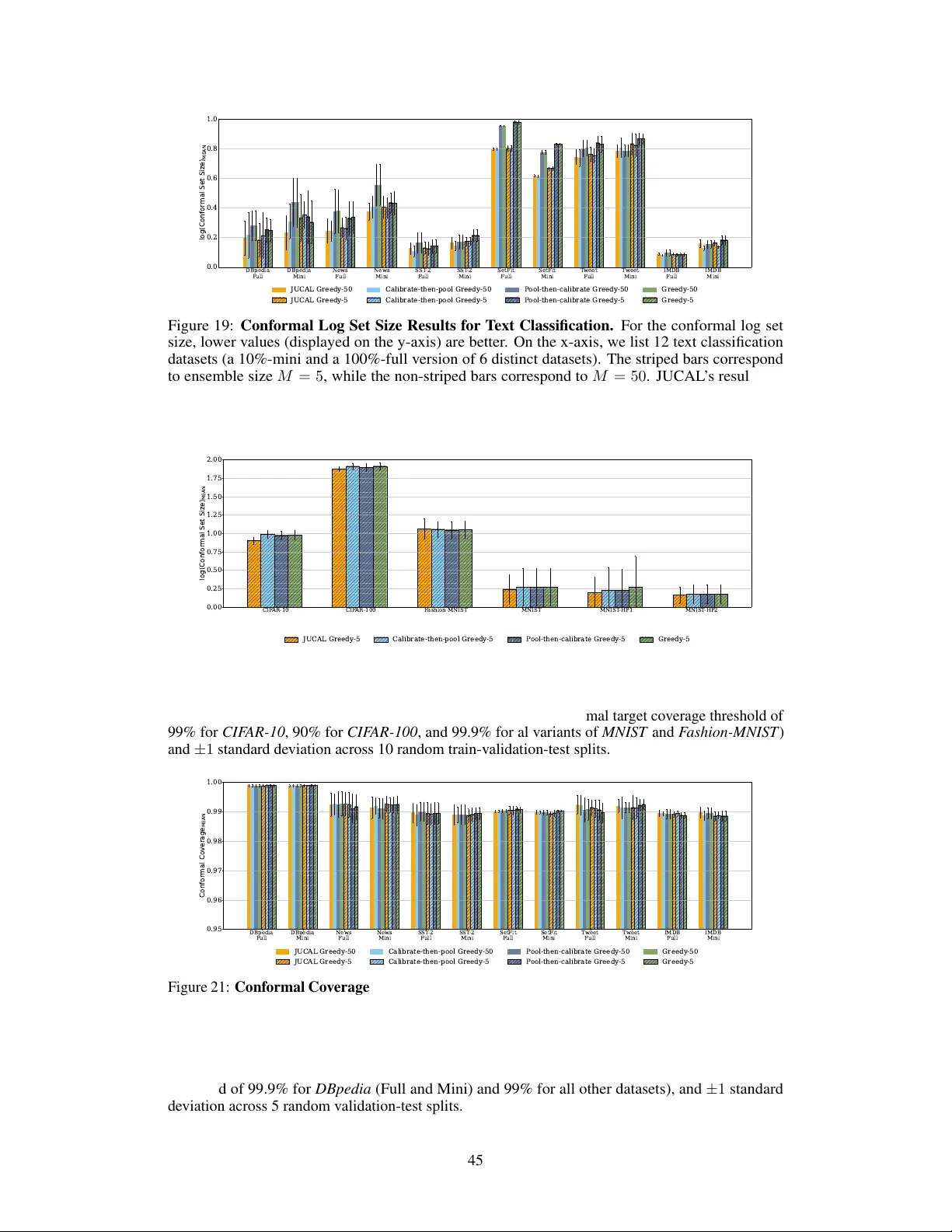
JUCAL: J ointly Calibrating Aleatoric and Epistemic Uncertainty in Classiﬁcation T asks Jak ob Heiss ∗ UC Berkeley jakob.heiss@berkeley.edu Sören Lambr echt ∗ ETH Zurich sorenlambrecht@gmail.com Jak ob W eissteiner † UBS Zurich jakob.weissteiner@gmx.at Hanna W utte † UBS Zurich wutte.hanna@gmail.com Žan Žuri ˇ c Kaiju W orldwide zan.zuric@gmail.com Josef T eichmann ETH Zurich josef.teichmann@math.ethz.ch Bin Y u UC Berkeley binyu@berkeley.edu Abstract W e study post-calibration uncertainty for trained ensembles of classiﬁers. Specif- ically , we consider both aleatoric uncertainty (i.e., label noise) and epistemic uncertainty (i.e., model uncertainty). Among the most popular and widely used cal- ibration methods in classiﬁcation are temperature scaling (i.e., pool-then-calibrate ) and conformal methods. Howe ver , the main shortcoming of these calibration methods is that they do not balance the proportion of aleatoric and epistemic uncer - tainty . Nev ertheless, not balancing epistemic and aleatoric uncertainty can lead to sev ere misrepresentation of predicti ve uncertainty , i.e., can lead to ov erconﬁdent predictions in some input regions while simultaneously being underconﬁdent in other input regions. T o address this shortcoming, we present a simple but po werful calibration algorithm Joint Uncertainty Calibration (JUCAL) that jointly calibrates aleatoric and epistemic uncertainty . JUCAL jointly calibrates two constants to weight and scale epistemic and aleatoric uncertainties by optimizing the ne gative log-likelihood (NLL) on the v alidation/calibration dataset. JUCAL can be applied to any trained ensemble of classiﬁers (e.g., transformers, CNNs, or tree-based methods), with minimal computational ov erhead, without requiring access to the models’ internal parameters. W e experimentally ev aluate JUCAL on various te xt classiﬁcation tasks, for ensembles of v arying sizes and with dif ferent ensembling strategies. Our experiments show that JUCAL signiﬁcantly outperforms SOT A calibration methods across all considered classiﬁcation tasks, reducing NLL and predicti ve set size by up to 15% and 20%, respecti vely . Interestingly , ev en applying JUCAL to an ensemble of size 5 can outperform temperature-scaled ensembles of size up to 50 in terms of NLL and predictiv e set size, resulting in up to 10 times smaller inference costs. Thus, we propose JUCAL as a new go-to method for calibrating ensembles in classiﬁcation. 3 ∗ First author equal contribution. † Second author equal contribution 3 This is a preliminary version of an ongoing project; e xpanded ev aluations are currently in progress. 1 Introduction Machine learning (ML) systems ha ve been widely adopted in v arious applications, and the rate of adoption is only increasing with recent adv ancements in generati v e artiﬁcial intelligence (AI) [ 10 ]. Deep learning (DL) models, often at the core of ML systems, can learn meaningful representations by mapping complex high-dimensional data to lo wer -dimensional feature spaces [ 56 ]. Howe ver , many DL frame works only pro vide point predictions without accompanying uncertainty estimates, which poses signiﬁcant challenges in high-stakes decision-making scenarios [50, 81]. Uncertainty in ML is commonly categorized into aleatoric and epistemic uncertainty [ 23 , 59 , 46 , 50 ]. Aleatoric uncertainty refers to the inherent randomness in the data-generating process, such as noise or class ov erlap, which cannot be reduced by collecting more training observ ations and is therefore often considered irreducible 4 . In contrast, epistemic uncertainty , also referred to as model uncertainty , captures the model’ s lack of knowledge about the data-generating process, typically arising from limited number of training observations. It is considered reducible through collecting additional training observations or by incorporating stronger inductiv e biases, such as priors or architectural constraints. For more details on these concepts, see Section A. While we adopt the con ventional distinction between aleatoric and epistemic uncertainty , we note that this dichotomy reﬂects a theoretical abstraction. In real-world data science workﬂo ws, uncertainty arises from a broader range of sources, including modeling choices, data collection, data prepro- cessing, and domain assumptions. While most aspects of modeling choices fall into the cate gory of epistemic uncertainty , some aspects of the data collection process and imputation methods for missing values do not alw ays ﬁt well into either of these tw o categories. The Pr edictability-Computability- Stability (PCS) frame work for v eridical data science of fers a more comprehensive vie w of the data science life cycle (DSLC) and highlights the importance of stability in analytical decisions [ 88 , 89 ]. Section C.1 provides more details on PCS and ho w it relates to JUCAL. In classiﬁcation, neural networks (NNs) typically output class probabilities via the softmax outputs. Howe ver , modern NNs often yield poorly calibrated probabilities, where the predicted conﬁdence scores do not reliably reﬂect the true conditional likelihoods of the labels [ 31 ]. Calibration, therefore, is critical to ensure that uncertainty estimates are meaningful and trustw orthy , particularly in high- stakes or safety-critical applications [ 66 , 53 ]. In the PCS frame work [ 88 ], calibration directly supports the Pr edictability principle, acting as a statistical reality check to ensure that model outputs are well aligned with empirical results. Calibration can prevent a model from being on averag e too over - or underconﬁdent on a gi ven dataset. Howe ver , a more challenging task is to develop models that accurately adapt their uncertainty for differ ent data points. F or example, in the absence of strong prior kno wledge, one w ould e xpect higher epistemic uncertainty for inputs that are far out-of-distribution (OOD), where predictiv e accuracy typically deteriorates [ 28 , 37 ]. 5 Con v ersely , lower epistemic uncertainty is expected for inputs densely surrounded by training data. Howe ver , modern NNs typically do not exhibit this sensiti vity: softmax outputs tend to remain ov erconﬁdent far from the training data, and standard calibration techniques cannot change the relati ve ranking of uncertainties across inputs (see Figure 1(a)). As a result, ev en calibrated softmax outputs are often o verconﬁdent OOD and underconﬁdent in-distrib ution (while achieving mar ginal calibration a v eraged ov er the v alidation set). Although many methods exist for uncertainty estimation in DL, Gustafsson et al. [32] suggest that deep ensembles (DEs), introduced by Lakshminarayanan et al. [55] , should be considered the go-to method. Additionally to incorporating aleatoric uncertainty via softmax outputs, DEs also incorporates epistemic uncertainty via ensemble div ersity (which is typically higher OOD). They achiev e this simply by averaging the softmax outputs of multiple trained NNs. Howe v er , they are inherently not well-calibrated [54, 72, 86]. 4 In practice, aleatoric uncertainty can sometimes be reduced by reformulating the problem, e.g., by including additional informative cov ariates. For example, a model predicting whether houses will sell within a month based only on price and square footage faces high aleatoric uncertainty . Man y houses with identical features ha ve different outcomes. Adding a co v ariate like location can e xplain much of this v ariance, reducing the a verage aleatoric uncertainty across the dataset. 5 This behavior depends on the assumptions encoded in the model (prior knowledge). For example, if the true logits are known to be a linear function of x , extrapolation beyond the training domain in certain directions may be justiﬁed with high conﬁdence. 2 4 2 0 2 F eature 1 4 2 0 2 4 F eature 2 Single Neural Network Train Class 0 Train Class 1 4 2 0 2 F eature 1 4 2 0 2 4 F eature 2 Deep Ensemble Train Class 0 Train Class 1 4 2 0 2 F eature 1 4 2 0 2 4 F eature 2 P ool-then-Calibrate ( =1.009) Train Class 0 Train Class 1 4 2 0 2 F eature 1 4 2 0 2 4 F eature 2 JUCAL (c1=1.011, c2=4.211) Train Class 0 Train Class 1 0.0 0.2 0.4 0.6 0.8 1.0 P r e d i c t i v e P r o b a b i l i t y o f Y = 1 | X = x (a) (b) (c) (d) Figure 1: Predictiv e probability estimation for a synthetic 2D binary classiﬁcation task. (a) Softmax outputs from a single NN. (b) Deep Ensemble. (c) & (d) show the same ensemble as in (b) b ut with different calibration algorithms applied to it. In all cases, the uncertainty peaks near the decision boundary , but only JUCAL suf ﬁciently accounts for epistemic uncertainty by widening the uncertain region (bright colors) as the distance to the training data increases. This reﬂects the model’ s limited knowledge in data-sparse re gions, highlighting the ensemble’ s ability to distinguish between aleatory and epistemic components. Again, standard post-hoc calibration techniques, such as conformal methods [ 4 ] or the pool-then-calibrate temperature scaling approach [ 72 ], mitigate the tendency of DEs to be on aver age too under- or overconﬁdent; ho we v er , the y do not address the balancing of aleatoric and epistemic uncertainty during calibration. The epistemic uncertainty’ s dependenc y on its hyperparameters can be highly unstable. For example, Y u & Barter [89] , Agarwal et al. [2] recommend training ev ery ensemble member on a different bootstrap sample of the data. This increases the ensemble’ s diversity and thus the estimated epistemic uncertainty . On the other hand, Lakshminarayanan et al. [55] recommend training ev ery ensemble member on the whole training dataset, which is expected to reduce the di versity of the ensemble. Also, other hyperparameters such as batch-size, weight-decay , learning-rate, dropout-rate, and initialization affect the diversity of the ensemble. In practice, all these hyperparameters are usually chosen without considering the ensemble di versity , and we cannot expect that they result in the right amount of epistemic uncertainty . There is also no reason to believ e that the miscalibration of DEs’ aleatoric and DEs’ epistemic uncertainty has to be aligned: For example, if we regularize too much, DEs usually ov erestimate the aleatoric uncertainty and underestimate the epistemic uncertainty . In such cases, decreasing the temperature of the predictive distrib ution results in overconﬁdent OOD predictions, while increasing it leads to underconﬁdence in regions dominated by aleatoric uncertainty . Classical temperature scaling cannot resolve this imbalance between the two types of uncertainty . T o address this shortcoming , we propose JUCAL , a no vel method speciﬁcally for classiﬁcation that jointly calibrates both aleatoric and epistemic uncertainty . Unlike standard post-hoc calibration approaches, our method explicitly balances these tw o uncertainty types during calibration, resulting in well-calibrated point-wise predictions (visualized in Figure 1(b)) and informativ e decomposed uncertainty estimates. Our algorithm can be easily applied to any already trained ensemble of models that output “probabilities”. Our experiments across multiple text-classiﬁcation datasets demonstrate that our approach consistently outperforms existing benchmarks in terms of NLL (up to 15%), predictiv e set size (up to 20% giv en the same cov erage), and A OROC = (1 − A UR OC ) (up to 40%). Our method reduces the inference cost of the best-performing ensemble proposed in Arango et al. [5] by a factor of about 10, while simultaneously improving the uncertainty metrics. 3 2 Related W ork Bayesian methods, such as Bayesian NNs (BNNs) [ 67 , 27 ], estimate both epistemic and aleatoric uncertainty by placing a prior ov er the NN’ s weights. If the true prior were known, the posterior predictiv e distrib ution would theoretically be well calibrated in a Bayesian sense. Howe v er , in practice, the prior is often unkno wn or misspeciﬁed, and thus BNNs are not guaranteed to produce calibrated predictions. W e note that our algorithm can easily be extended to BNNs. As an alternativ e, DEs, introduced by Lakshminarayanan et al. [55] , hav e demonstrated competiti ve or superior performance compared to BNNs across sev eral metrics [ 1 , 32 , 70 ]. DEs, from a Bayesian perspectiv e, approximate the posterior predicti v e distrib ution by av eraging predictions (i.e. softmax outputs) from multiple models trained from independent random initializations. Howe ver , like BNNs, DEs are not inherently well-calibrated and often require additional calibration to ensure reliable uncertainty estimates [6]. Guo et al. [31] suggest temperature scaling as a simple, yet effecti v e, calibration method for mod- ern NNs. Rahaman et al. [72] criticize the calibration properties of ensembles and recommend pool-then-calibrate , aggre gating ensemble member predictions before applying temperature scaling to the combined log-probabilities, using a proper scoring rule such as NLL. Although this approach can improv e the calibration of DEs [ 72 ], it relies on a single calibration parameter to scale the total uncertainty , without using separate parameters to explicitly account for aleatoric and epistemic uncertainty . Thus, pool-then-calibrate implicitly assumes that aleatoric and epistemic uncertainty are both equally miscalibrated. In contrast, our algorithm calibrates both epistemic and aleatoric uncertainty with individual scaling factors, allowing us to increase one of them while simultaneously reducing the other one. Recently , Azizi et al. [7] hav e demonstrated that the conceptual idea of using two calibration constants to balance epistemic and aleatoric uncertainty can also be successfully applied to regression while facing dif ferent technical challenges. See Section C for further related work. 3 Problem Setup Consider the setting of supervised learning, where we are giv en a training dataset D train = { ( x 1 , y 1 ) , . . . , ( x N , y N ) } ⊂ X × Y , where the pairs ( x i , y i ) are assumed to be independent and identically distributed (i.i.d.) and Y = { 1 , . . . , K } consists of K classes. Similar to the setup de- scribed in Lakshminarayanan et al. [55] , let { f m } M m =1 be an ensemble of M independently 6 trained NN classiﬁers and let { θ m } M m =1 denote the parameters of the ensemble. For each x ∈ X , each ensemble member f m , followed by a softmax acti vation, produces a probability-vector Softmax ( f m ( x )) = p ( y | x , θ m ) = ( p ( y = 0 | x , θ m ) , . . . , p ( y = K − 1 | x , θ m )) in the simplex △ K − 1 , as visualized in Figure 2 (this can be seen as an approximation of a Bayesian posterior as described in Section A.2.2). A classical DE would no w simply av erage these probability vectors to obtain a predicti v e distribution o v er the K classes for a giv en input datapoint x N +1 : p  y | x N +1 , { θ m } M m =1  = 1 M M X m =1 p ( y | x N +1 , θ m ) ∈ △ K − 1 . (1) 3.1 Aleatoric and Epistemic Uncertainty There are fundamentally different reasons to be uncertain. Case 1: If each ensemble of the M ensemble members outputs a probability vector in the center of the simplex without fav oring any class, you should be uncertain (aleatoric uncertainty; similar to Figure 2(c)). 7 Case 2: If each ensemble member outputs a probability vect or in a corner of the simple x, where each corner is chosen by M K ensemble members, you should be uncertain too (epistemic uncertainty; similar to Figure 2(d)). 8 Both 6 The neural networks are not statistically independent if the dataset D is treated as a random variable, since all models are trained on the same D . Howe v er , they can be considered conditionally independent gi ven D , due to independent random initialization and data shufﬂing at the be ginning of each training epoch. 7 This is analogous to multiple doctors telling you that they are too uncertain to make a diagnosis. 8 This is analogous to multiple doctors telling you highly contradictory diagnoses. 4 Class 0 Class 1 Class 0 Class 1 Class 2 Class 0 Class 1 Class 2 Class 0 Class 1 Class 2 Class 0 Class 1 Class 2 (a) (b) (c) (d) (e) Figure 2: Scatter plots of ensemble members’ softmax outputs for (a) binary ( K = 2) and (b-e) ternary ( K = 3 ) classiﬁcation. Each subplot shows a different possibility of how the M = 50 predictions could be arranged for a ﬁxed input point x . Each point represents a probability vector p ( y | x, θ m ) ov er K classes estimated by an ensemble member . (a)&(b) low total predictive uncertainty; (c) very high aleatoric and low epistemic uncertainty; (d) low aleatoric and v ery high epistemic uncertainty; (d)&(e) high epistemic uncertainty . Theoretically (d) claims that the aleatoric uncertainty is certainly lo w , while (e) is uncertain about the aleatoric uncertainty , but in practice, both (d)&(e) should usually be simply interpreted as high epistemic uncertainty (see Remark A.1). cases result in a predictiv e distrib ution p that is uniform over the K classes. Howe ver , in practice, this can lead to very dif ferent decisions. The diversity of the ensemble members describes the epistemic uncertainty , while each indi vidual ensemble member estimates the aleatoric uncertainty . There are multiple different approaches to quantify them mathematically (see Section A.2). In our method, we calibrate these two uncertainty components separately . 4 Jointly Calibrating Aleatoric and Epistemic Uncertainty 4.1 T emperature Scaling For an y probability vector p ∈ △ K − 1 , one can transform p by temperature scaling p TS ( T ) := Softmax  Softmax − 1 ( p ) /T  , with logits f TS ( T ) := Softmax − 1 ( p ) /T , which mov es p tow ards the center of the simple x for temperatures T > 1 and aw ay from the center tow ards the corners for T < 1 , where Softmax ( z ) = 1 P K j =1 exp( z j ) (exp( z 1 ) , . . . , exp( z K )) . P ool-then-calibrate applies temperature scaling to the predictiv e probabilities p from Equation (1) . This allows to increase the total predicti ve uncertainty with T > 1 or reducing it with T < 1 . Calibrate-then-pool applies temperature scaling on each individual ensemble-member p ( y | x , θ m ) before av eraging them. Thus, Calibrate-then-pool mainly adjusts the aleatoric uncertainty . 4.2 JUCAL JUCAL uses two calibration constants c 1 and c 2 . JUCAL applies temperature scaling on each indi vidual ensemble-member p ( y | x , θ m ) = Softmax ( f m ( x )) with temperature T = c 1 , resulting in temperature-scaled logits f TS ( c 1 ) m = f m c 1 ∈ R K , as in Calibrate-then-pool . This allo ws us to increase the estimated aleatoric uncertainty by setting c 1 > 1 and to reduce it by setting c 1 < 1 . Howe ver , c 1 is not sufﬁcient to calibrate the epistemic uncertainty . Therefore, we introduce a second calibration mechanism for calibrating the epistemic uncertainty via c 2 . Concretely , c 2 adjusts the ensemble-diversity of the already temeperature-scaled logits f TS ( c 1 ) m ( x ) without changing their mean ¯ f TS ( c 1 ) ( x ) := 1 M P M m =1 f TS ( c 1 ) m ( x ) . I.e., the diversity- adjusted ensemble-logits f JUCAL ( c 1 ,c 2 ) m ( x ) := (1 − c 2 ) ¯ f TS ( c 1 ) ( x ) + c 2 f TS ( c 1 ) m ( x ) increase their distance to their mean ¯ f TS ( c 1 ) ( x ) for c 2 > 1 and decrease it for c 2 < 1 . By applying Softmax we obtain an ensemble of M probability-vectors p JUCAL ( c 1 ,c 2 ) m ( x ) = Softmax  f JUCAL ( c 1 ,c 2 ) m ( x )  ∈ △ K − 1 . By combining these steps and av eraging, JUCAL obtains the calibrated predicti ve distrib ution ¯ p JUCAL ( c 1 ,c 2 ) ( x ) := 1 M M X m =1 Softmax  (1 − c 2 ) c 1 ¯ f ( x ) + c 2 c 1 f m ( x )  (2) 5 from the uncalibrated logits f m ( x ) of the M ensemble members and their mean ¯ f := P M m =1 f m ( x ) . In practice, we usually don’t kno w a priori ho w to set c 1 and c 2 . Hence, JUCAL picks ( c ∗ 1 , c ∗ 2 ) ∈ arg min ( c 1 ,c 2 ) ∈ (0 , ∞ ) × [0 , ∞ ) NLL ( ¯ p JUCAL ( c 1 ,c 2 ) , D cal ) (3) that minimize the NLL ( p, D cal ) := − 1 |D cal | P ( x,y ) ∈D cal log p ( y | x ) on a calibration dataset D cal . The NLL is a proper scoring rule, and re w ards lo w uncertainty for correct predictions and strongly penalizes lo w uncertainty for wrong predictions. In our experiments, we are reusing the v alidation dataset D v al as a calibration dataset while ev aluating our results on a separate test set D test . For a pseudo-code implementation of JUCAL, see Algorithm 1. Algorithm 1: JUCAL (simpliﬁed). See Algorithm 2 for a faster implementation. Input : Ensemble E = ( f 1 , . . . , f M ) , calibration set D cal (e.g., D cal = D v al ), grid C for candidate values ( c 1 , c 2 ) 1 Initialize best NLL ← ∞ and ( c ∗ 1 , c ∗ 2 ) arbitrarily 2 f oreach ( c 1 , c 2 ) ∈ C do 3 current_NLL ← 0 4 for each ( x, y ) ∈ D cal do 5 for each m = 1 , . . . , M do 6 f TS m ( x ) ← f m ( x ) /c 1 ▷ T emperature scaling 7 for each m = 1 , . . . , M do 8 f JUCAL m ( x ) ← (1 − c 2 ) · 1 M P M m ′ =1 f TS m ′ ( x ) + c 2 · f TS m ( x ) ▷ Div ersity adjustment 9 ¯ p JUCAL ( x ) ← 1 M P M m =1 Softmax ( f JUCAL m ( x )) 10 current_NLL ← current_NLL + NLL ( ¯ p JUCAL ( x ) , y ) 11 if curr ent_NLL < best_NLL then 12 best_NLL ← current_NLL 13 ( c ∗ 1 , c ∗ 2 ) ← ( c 1 , c 2 ) retur n : ( c ∗ 1 , c ∗ 2 ) 4.3 Further Intuition on JUCAL In Figure 3, we sho w a simple toy e xample where all the ensemble members manage to quite precisely learn the true conditioned class-probability within the body of the distribution, b ut not in data-scarce regions. Also, the disagreement of the ensemble logits increases in data-scarce regions, indicating a higher epistemic uncertainty in these regions. Howe v er , the amount by which disagreement increases in these regions is too low in this e xample, while at the same time, the aleatoric uncertainty is slightly o verestimated (e.g., at x = − π 2 ). This leads to overconﬁdence OOD (i.e., outside [ − 7 , 7] ) and slight underconﬁdence in the body of the distribution. Pool-then-calibrate can only globally increase or decrease the uncertainty , which cannot resolve this problem. In contrast, JUCAL can simply increase the ensemble div ersity via c 2 ≫ 1 and simultaneously decrease the aleatoric uncertainty via c 1 < 1 , resulting in reasonable input-conditional predictive uncertainty across the entire range of x ∈ [ − 10 , 10] . In the lo w epistemic-uncertainty re gions, the logits of different ensemble members almost perfectly agree; therefore, linearly scaling up their disagreement by c 2 does only hav e a small effect. Con versely , in regions where disagreement of pre-calibrated logits is already elev ated, scaling this further up by c 2 has a large effect. This way , c 2 can more selectively calibrate the epistemic uncertainty without manipulating the aleatoric uncertainty too much. 5 Results In this section, we empirically ev aluate JUCAL based on a comprehensiv e set of experiments. In Section 5.1 we describe the experimental setup and in Section 5.2 the e xperimental results. 6 5.1 Experimental Setup Arango et al. [5] introduce a comprehensi ve metadataset containing prediction probabilities from a large number of ﬁne-tuned lar ge language models (LLMs) on six text classiﬁcation tasks. For each task, predictions are provided on both v alidation and test splits. The underlying models include GPT2, BER T -Large, B AR T -Large, ALBER T -Lar ge, and T5-Large, spanning a broad range of architectures and parameter counts, from 17M to 770M parameters. This metadataset is particularly valuable as it allows us to use already ﬁnetuned models for our experiments. Arango et al. [5] used 3800 GPU hours to ﬁne-tune these models, allowing us to isolate and study the effects of aggre gation and calibration strategies independently of model training. In comparison, applying JUCAL to these expensi v ely ﬁne-tuned models only requires a few CPU-minutes. Six full-sized datasets and six reduced mini-datasets were used. Additional details about the metadataset are provided in T able 10. 5.1.1 Evaluation Metrics and Benchmarks Model performance is ev aluated using the av erage NLL, which is commonly used in related work and also reported by Arango et al. [5] for their ensemble methods. It is computed as NLL ( p, D test ) := − P ( x,y ) ∈D test log p ( y | x ) . In addition, we report A ORA C = 1 − A URA C , representing the area ov er the rejection-accuracy curve. Each point on this curve gi ves the accuracy on a subset of the dataset, where the model is most certain, i.e., the model is allowed to reject answering questions for which it estimates high uncertainty . The A ORA C is equal to the a verage misclassiﬁcation rate, av eraged over all different rejection rates. As a third metric, we report A OR OC = 1 − A UROC , representing the area ov er the receiver -operator -curve (R OC) . Here, the A UROC is computed by av eraging the one-vs-rest A UR OC scores obtained for each class. Both A ORA C and A OR OC measure how well the model is able to rank the uncertainty of dif ferent input datapoints. As a fourth metric, we e v aluate the a verage size of the prediction set required to co ver the true label with high conﬁdence (cov erage threshold). For most datasets we use a 99% coverage threshold, but for DBpedia we increase this to 99.9% due to the high accuracy of the model predictions. Among the ensemble methods presented by Arango et al. [5] , Greedy-50 , a greedy algorithm that iterati vely adds the model providing the largest performance gain (in terms of NLL ( p, D v al ) ) until an ensemble of size 50 is formed, achiev es the best o verall performance. The authors demonstrate that Gr eedy-50 outperforms se v eral ensemble construction strategies, including: Single Best , which selects the single model with the best validation performance; Random-M , which builds an ensemble by randomly sampling M models; T op-M , which selects the M models with the highest validation scores; Model A verage (MA) , which averages predictions from all models using uniform weights without model selection. They ev aluated M = 5 and M = 50 , and Gr eedy-50 had the best performance in terms of NLL across all 12 datasets. Giv en its strong empirical performance, we adopt Greedy-50 as our benchmark. Additionally , we adopt Gr eedy-5 as another benchmark, due to its up to 10 times lower computational prediction costs, 10.0 7.5 5.0 2.5 0.0 2.5 5.0 7.5 10.0 X values 0.0 0.2 0.4 0.6 0.8 1.0 Probability (Class 1) Deep Ensemble & P ool-then-Calibrate ( =0.862) E n s e m b l e m e m b e r p ( y = 1 | x , m ) E n s e m b l e m e a n p P o o l - t h e n - C a l i b r a t e p c a l T r u e p ( y = 1 | x ) T r a i n i n g o b s e r v a t i o n s ( x , y ) 10.0 7.5 5.0 2.5 0.0 2.5 5.0 7.5 10.0 X values Probability (Class 1) JUCAL (c1=0.810, c2=7.041) JUCAL ensemble member J U C A L e n s e m b l e m e a n p J U C A L ( c 1 , c 2 ) ( x ) T r u e p ( y = 1 | x ) T r a i n i n g o b s e r v a t i o n s ( x , y ) Figure 3: Binary classiﬁcation example with X ∼ N (0 , 1) . The ensemble logits strongly agree in the center of the distribution x ∈ [ − 2 , 2] , but disagree more as one mov es aw ay from the center . The two subplots sho w the same ensemble before and after applying JUCAL to it. 7 which can be crucial in certain applications. For both of these ensembles, we compare three different calibration strategies: JUCAL (Algorithm 1), pool-then-calibrate , and no calibration. 5.2 Experimental Results Figures 4 – 5 present the performance of different calibration techniques on the Greedy-50 and Greedy-5 ensembles across six metrics. For detailed tables and further ablation studies, see Section F. Arango et al. [5] demonstrated the strength of the Greedy-50 ensemble, which we further improve with our calibration method at a ne gligible computational cost (see Section H). The state-of-the-art pool-then-calibrate method improves NLL (Figures 4(a)&5(a)) but only rarely the other metrics. Our proposed method, JUCAL, simultaneously improv es all four metrics compared to both the uncalibrated and state-of-the-art calibrated ensembles across most datasets. W e observe similar performance gains for JUCAL on the smaller Gr eedy-5 ensembles. In line with Arango et al. [5] , the uncalibrated Greedy-50 ensemble consistently outperforms Gr eedy- 5 in terms of test-NLL, b ut at an approximately 10x higher computational inference cost. Howe ver , applying JUCAL to Gr eedy-5 requires only a negligible one-time computational in v estment and maintains its low inference costs, while achieving superior performance to both the uncalibrated Gr eedy-50 and the pool-then-calibrate Greedy-50 across most datasets and metrics. This demonstrates JUCAL ’ s ability to signiﬁcantly reduce inference costs without sacriﬁcing predicti ve quality . W e recommend JUCAL Gr eedy-5 for cost-sensitiv e applications and JUCAL Gr eedy-50 for scenarios where ov erall performance is the top priority . Figure 4(a) shows the NLL on a held-out test set D test , our primary metric due to its property as a strictly proper scoring rule. JUCAL consistently improv es the NLL of the Greedy-50 ensemble, outperforming all other non-JUCAL ensembles across all 12 datasets, with most improv ements being statistically signiﬁcant (see T ables 2 and 6 in Section F). Even more notably , for the smaller Greedy-5 ensembles, JUCAL achie ves the best average test-NLL among all size-5 ensembles, with NLL reductions up to 30%. For example, on DBpedia, JUCAL Greedy-5 trained on just 10% of the data achiev es a lower av erage NLL than all non-JUCAL ensembles, including the 10x larger ensembles trained on the full dataset. This demonstrates that JUCAL offers a more effecti v e and computationally ef ﬁcient path to improving performance than simply scaling up the training data or ensemble size. Figure 4(b)&(c) show the A ORA C = 1 − A URAC and A OR OC = 1 − A UROC , respectively , as deﬁned in Section 5.1.1. The pool-then-calibrate method sho ws no ef fect for these metrics. This is expected because these metrics measure the relati ve uncertainty which is inv ariant to monotonic transformations. They assess whether positiv e examples hav e higher certainty than negativ e ones, irrespectiv e of absolute uncertainty level. In contrast, JUCAL and calibrate-then-pool consistently improv e A OROC across all datasets, with statistically signiﬁcant gains in most cases. This sho ws that JUCAL activ ely impro ves the relati v e uncertainty ranking of the model. Figure 4(d), presents the predicti ve set size results. JUCAL and calibrate-then-pool achieve signiﬁ- cantly smaller predicti ve sets. Already , a reduction in set size from 1.2 to 1.1 can equate to halving the costs of human interventions, if a set size of one corresponds to zero human interv ention. 5.3 JUCAL ’ s Disentanglement Into Aleatoric and Epistemic Uncertainty . Figure 6 demonstrates that the epistemic uncertainty estimated by JUCAL Gr eedy-50 substantially decreases as more training observations are collected for each of the 6 datasets, and for 5 out of 6 datasets in the case of JUCAL Gr eedy-5 . Con versely , the estimated aleatoric uncertainty usually does not show any systematic tendency to decrease as more training observations are collected. These results align well with the theoretical understanding that epistemic uncertainty is reducible by collecting more training observations and aleatoric uncertainty is not. W e used Equations (6) and (7) from Section A.2.1 to compute the values presented in Figure 6, while there w ould be other alternativ es too. More research is needed to interpret dif ferent scales of estimated epistemic and aleatoric uncertainty across different datasets and dif ferent ensembles to better estimate the potential beneﬁts of collecting more data to guide efﬁcient data collection. For more details, see Section A.3. 8 6 Conclusion W e ha ve presented a simple yet effecti ve method that jointly calibrates both aleatoric and epistemic uncertainty in DEs. Unlike standard post-hoc approaches such as temperature scaling, our method addresses both absolute and relativ e uncertainty through structured ﬁtting of prediction distributions. Experiments on sev eral datasets sho w that our method consistently and often signiﬁcantly improves upon state-of-the-art baselines, including Greedy-50 and P ool-then-Calibrate Gr eedy-50 , and is almost nev er signiﬁcantly outperformed by any of the baselines on any e v aluated metric. Our method is remarkably stable and reliable, making it a safe and practical addition to any classiﬁcation task. It can also be used to reduce inference costs without sacriﬁcing predicti ve performance or uncertainty quality by compensating for the weakness of Gr eedy-5 . Limitations and future work: So far , our empirical ev aluation focused on text classiﬁcation with ﬁne-tuned LLMs and image classiﬁcation with CNNs, using rather large calibration datasets. Future work includes ev aluating JUCAL on other data modalities and models and extending it to Chatbots. 9 0.6 0.8 1.0 1.2 1.4 1.6 N L L M E A N ( n o r m a l i z e d ) 0.00 0.02 0.04 0.06 0.08 0.10 0.12 A O R A C M E A N 1 0 4 1 0 3 1 0 2 1 0 1 A O R O C M E A N ( l o g s c a l e ) 1.0 1.2 1.4 1.6 1.8 2.0 2.2 2.4 2.6 2.8 S e t S i z e M E A N 0.00 0.05 0.10 0.15 0.20 0.25 0.30 B r i e r S c o r e M E A N DBpedia Full DBpedia Mini News Full News Mini S ST -2 Full S ST -2 Mini SetFit Full SetFit Mini T weet Full T weet Mini IMDB Full IMDB Mini 0.00 0.05 0.10 0.15 0.20 0.25 M i s c l a s s i f i c a t i o n M E A N JUCAL Greedy-50 JUCAL Greedy-5 Calibrate-then-pool Greedy-50 Calibrate-then-pool Greedy-5 P ool-then-calibrate Greedy-50 P ool-then-calibrate Greedy-5 Greedy-50 Greedy-5 (a) (b) (c) (d) (e) (f) Figure 4: T ext Classiﬁcation Results. F or each of the six subplots, lower values of the metrics (displayed on the y-axis) are better . On the x-axis, we list 12 text classiﬁcation datasets (a 10%- mini and a 100%-full v ersion of 6 distinct datasets). The striped bars correspond to ensemble size M = 5 , while the non-striped bars correspond to M = 50 . JUCAL ’ s results are yellow . For all six metrics (deﬁned in Section 5.1.1), we show the a v erage and ± 1 standard deviation across 5 random validation-test splits. (a) NLL normalized by the mean of JUCAL Greedy-50 on the corresponding full dataset; (b) A ORA C = 1 − A URA C ; (c) A OROC = 1 − A UR OC ; (d) A verage set size for the cov erage threshold of 99.9% for DBpedia (Full and Mini) and 99% for all other datasets; (e) Brier Score ; (f) Misclassiﬁcation Rate = 1 − Accuracy . For more detailed results, see the corresponding tables in Section F. 10 0.8 0.9 1.0 1.1 1.2 1.3 N L L M E A N ( n o r m a l i z e d ) 0.00 0.05 0.10 0.15 0.20 A O R A C M E A N 1 0 5 1 0 4 1 0 3 1 0 2 1 0 1 A O R O C M E A N ( l o g s c a l e ) 1 2 3 4 5 6 7 S e t S i z e M E A N CIF AR-10 CIF AR-100 F ashion-MNIST MNIST MNIST -HP1 MNIST -HP2 0.0 0.1 0.2 0.3 0.4 0.5 0.6 B r i e r S c o r e M E A N CIF AR-10 CIF AR-100 F ashion-MNIST MNIST MNIST -HP1 MNIST -HP2 0.0 0.1 0.2 0.3 0.4 M i s c l a s s i f i c a t i o n M E A N JUCAL Greedy-5 Calibrate-then-pool Greedy-5 P ool-then-calibrate Greedy-5 Greedy-5 (a) (b) (c) (d) (e) (f) Figure 5: Image Classiﬁcation Results. For each of the six subplots, lower v alues of the metrics (displayed on the y-axis) are better . On the x-axis, we list distinct image classiﬁcation datasets (and two hyperparameter -ablation studies for MNIST). JUCAL ’ s results are yellow . For all six metrics (deﬁned in Section 5.1.1), we show the av erage and ± 1 standard deviation across 10 random train-validation-test splits. (a) NLL normalized by the mean of JUCAL Greedy-5; (b) A ORA C = 1 − A URA C ; (c) A OROC = 1 − A UR OC ; (d) A verage set size for the cov erage threshold of 99% for CIF AR-10 , 90% for CIF AR-100 , and 99.9% for al variants of MNIST and F ashion-MNIST ; (e) Brier Score ; (f) Misclassiﬁcation Rate = 1 − Accuracy . DBpedia Full DBpedia Mini News Full News Mini S ST -2 Full S ST -2 Mini SetFit Full SetFit Mini T weet Full T weet Mini IMDB Full IMDB Mini 0.0 0.1 0.2 0.3 0.4 0.5 U n c e r t a i n t y M E A N Epistemic (JUCAL Greedy-50) Epistemic (JUCAL Greedy-5) Aleatoric (JUCAL Greedy-50) Aleatoric (JUCAL Greedy-5) Figure 6: Epistemic and Aleatoric Uncertainty (computed as in Section A.2.1) of JUCAL applied on Greedy-50 ensembles across six datasets in the metadataset. W e compare the full (100%) and the mini (10%) metadataset conﬁgurations for both epistemic and aleatoric uncertainty . Bars indicate the mean uncertainty , and error bars denote one standard deviation o ver random seeds. 11 Reproducibility Statement Our source code for all experiments is av ailable at https://github.com/anoniclr2/iclr26_ anon . Upon ﬁnal publication, we will provide a permanent public repository with an installable package. Acknowledgments W e thank Anthon y Ozerov for the insightful discussions. Jakob Heiss gratefully ackno wledges support from the Swiss National Science Foundation (SNSF) Postdoc.Mobility fellowship [grant number P500PT_225356] and the Department of Statistics at UC Berkele y . He also wishes to thank the Department of Mathematics at ETH Zürich where the project’ s early ideas originated. Sören Lambrecht gratefully acknowledges Kaiju W orldwide for supporting this work, as parts of this project were conducted during his time there, and thanks Aitor Muguruza Gonzalez, Chief AI Ofﬁcer at Kaiju W orldwide, for v aluable discussions. Bin Y u gratefully acknowledges partial support from NSF grant DMS-2413265, NSF grant DMS 2209975, NSF grant 2023505 on Collaborative Research: Foundations of Data Science Institute (FODSI), the NSF and the Simons Foundation for the Collaboration on the Theoretical Foundations of Deep Learning through a wards DMS-2031883 and 814639, NSF grant MC2378 to the Institute for Artiﬁcial CyberThreat Intelligence and OperatioN (A CTION), and NIH (DMS/NIGMS) grant R01GM152718. The Use of Large Language Models (LLMs) W e used Large Language Models (LLMs), speciﬁcally ChatGPT and Gemini, to assist with improving the English writing on a sentence or paragraph lev el. The content and scientiﬁc ideas presented in the paper are entirely our own. Every suggestion provided by the LLM w as carefully re vie wed, iterated upon, and corrected by a human. W e conﬁrm that every sentence in the paper and the appendix has been checked and veriﬁed by a human author . In writing the code, we used standard LLM-based coding tools, speciﬁcally ChatGPT and Claude Code, to increase efﬁcienc y . These LLMs were used mainly for generating ﬁgures rather than for dev eloping core modules of the source code. All changes made with the help of an LLM were carefully revie wed before being committed to the GitHub repository . References [1] T aiga Abe, Estef any K elly Buchanan, Geoff Pleiss, Richard Zemel, and John P Cunningham. Deep ensembles work, but are they necessary? Advances in Neural Information Pr ocessing Systems , 35:33646–33660, 2022. [2] Abhineet Agarwal, Michael Xiao, Rebecca Barter, Omer Ronen, Boyu F an, and Bin Y u. Pcs-uq: Uncertainty quantiﬁcation via the predictability-computability-stability framew ork, 2025. URL https://arxiv.org/abs/2505.08784 . [3] Gustaf Ahdritz, Aravind Gollakota, P arikshit Gopalan, Charlotte Peale, and Udi W ieder . Prov- able uncertainty decomposition via higher -order calibration. In The Thirteenth International Confer ence on Learning Representations , 2025. URL https://openreview.net/forum? id=TId1SHe8JG . [4] Anastasios N Angelopoulos and Stephen Bates. A gentle introduction to conformal prediction and distribution-free uncertainty quantiﬁcation. arXiv pr eprint arXiv:2107.07511 , 2021. [5] Sebastian Pineda Arango, Maciej Jano wski, Lennart Puruck er , Arber Zela, Frank Hutter, and Josif Grabocka. Ensembling ﬁnetuned language models for text classiﬁcation. arXiv pr eprint arXiv:2410.19889 , 2024. 12 [6] Arsenii Ashukha, Alexander L yzhov , Dmitry Molchanov , and Dmitry V etrov . Pitfalls of in-domain uncertainty estimation and ensembling in deep learning. arXiv preprint arXiv:2002.06470 , 2020. [7] Ilia Azizi, Juraj Bodik, Jakob Heiss, and Bin Y u. Clear: Calibrated learning for epistemic and aleatoric risk, 2025. URL . [8] Mostafa Bakhouya, Hassan Ramchoun, Mohammed Hadda, and T awﬁk Masrour . Gaussian mixture models for training bayesian conv olutional neural networks. Evolutionary Intelligence , 17:1–22, January 2024. doi: 10.1007/s12065- 023- 00900- 9. [9] Sumanta Basu, Karl Kumbier , James B Brown, and Bin Y u. Iterati ve random forests to disco ver predictiv e and stable high-order interactions. Pr oceedings of the National Academy of Sciences , 115(8):1943–1948, 2018. [10] Alexander Bick, Adam Blandin, and David J Deming. The rapid adoption of generative ai. T echnical report, National Bureau of Economic Research, 2024. [11] Charles Blundell, Julien Cornebise, K oray Kavukcuoglu, and Daan W ierstra. W eight uncertainty in neural networks. In 32nd International Conference on Machine Learning (ICML) , 2015. URL http://proceedings.mlr.press/v37/blundell15.pdf . [12] Erez Buchweitz, João V itor Romano, and Ryan J. T ibshirani. Asymmetric penalties underlie proper loss functions in probabilistic forecasting, 2025. URL 2505.00937 . [13] Peter Bühlmann and Bin Y u. Analyzing bagging. The annals of Statistics , 30(4):927–961, 2002. [14] L. M. C. Cabezas, V . S. Santos, T . R. Ramos, and R. Izbicki. Epistemic uncertainty in conformal scores: A uniﬁed approach, 2025. URL . [15] Rich Caruana, Alexandru Niculescu-Mizil, Geof f Cre w , and Alex Ksik es. Ensemble selection from libraries of models. In Pr oceedings of the T wenty-F irst International Conference on Machine Learning , ICML ’04, pp. 18, New Y ork, NY , USA, 2004. Association for Computing Machinery . ISBN 1581138385. doi: 10.1145/1015330.1015432. URL https://doi.org/10. 1145/1015330.1015432 . [16] Rich Caruana, Art Munson, and Alexandru Niculescu-Mizil. Getting the most out of ensemble selection. In Pr oceedings of the Sixth International Confer ence on Data Mining , ICDM ’06, pp. 828–833, USA, 2006. IEEE Computer Society . ISBN 0769527019. doi: 10.1109/ICDM.2006.76. URL https://doi.org/10.1109/ICDM.2006.76 . [17] Matthew A. Chan, Maria J. Molina, and Christopher A. Metzler . Estimating epistemic and aleatoric uncertainty with a single model. In Pr oceedings of the 38th International Confer ence on Neural Information Pr ocessing Systems , NIPS ’24, Red Hook, NY , USA, 2025. Curran Associates Inc. ISBN 9798331314385. [18] Bai Cong, Nico Daheim, Y uesong Shen, Daniel Cremers, Rio Y okota, Mohammad Emtiyaz Khan, and Thomas Möllenhoff. V ariational low-rank adaptation using iv on, 2024. URL https://arxiv.org/abs/2411.04421 . [19] G. Cybenko. Approximation by superpositions of a sigmoidal function. Mathematics of Contr ol, Signals and Systems , 2(4):303–314, December 1989. ISSN 1435-568X. doi: 10.1007/ BF02551274. URL https://doi.org/10.1007/BF02551274 . [20] Erik Daxberger , Agustinus Kristiadi, Alexander Immer , Runa Eschenhagen, Matthias Bauer , and Philipp Hennig. Laplace redux - effortless bayesian deep learning. In M. Ranzato, A. Beygelzimer , Y . Dauphin, P .S. Liang, and J. W ortman V aughan (eds.), Advances in Neural Information Pr ocessing Systems , volume 34, pp. 20089–20103. Curran Associates, Inc., 2021. URL https://proceedings.neurips.cc/paper_files/paper/2021/file/ a7c9585703d275249f30a088cebba0ad- Paper.pdf . 13 [21] Stefan Depewe g, José Miguel Hernández-Lobato, Finale Doshi-V elez, and Steffen Udluft. Uncertainty decomposition in bayesian neural netw orks with latent v ariables. arXiv pr eprint arXiv:1706.08495 , 2017. [22] Stefan Depewe g, Jose-Miguel Hernandez-Lobato, Finale Doshi-V elez, and Steffen Udluft. Decomposition of uncertainty in bayesian deep learning for efﬁcient and risk-sensiti ve learning. In International confer ence on mac hine learning , pp. 1184–1193. PMLR, 2018. [23] Armen Der Kiureghian and Ove Ditlevsen. Aleatory or epistemic? does it matter? Structural safety , 31(2):105–112, 2009. [24] Raaz Dwiv edi, Y an Shuo T an, Briton Park, Mian W ei, K e vin Horgan, Da vid Madigan, and Bin Y u. Stable discovery of interpretable subgroups via calibration in causal studies. International Statistical Revie w , 88:S135–S178, 2020. [25] Michael Havbro Faber . On the treatment of uncertainties and probabilities in engineering decision analysis. Journal of Offshor e Mechanics and Arctic Engineering , 127(3):243–248, August 2005. ISSN 0892-7219, 1528-896X. doi: 10.1115/1.1951776. [26] Y arin Gal and Zoubin Ghahramani. Dropout as a Bayesian Approximation: Representing Model Uncertainty in Deep Learning. June 2015. URL . arXiv: 1506.02142. [27] Y arin Gal et al. Uncertainty in deep learning. 2016. [28] Saurabh Garg, Siv araman Balakrishnan, Zachary C Lipton, Behnam Neyshab ur , and Hanie Sedghi. Leveraging unlabeled data to predict out-of-distribution performance. arXiv preprint arXiv:2201.04234 , 2022. [29] T . Gneiting and A. E Raftery . Strictly proper scoring rules, prediction, and estimation. Journal of the American statistical Association , 102(477):359–378, 2007. [30] Alex Graves. Practical variational inference for neural networks. In Advances in neural information pr ocessing systems , pp. 2348–2356, 2011. URL http://papers.nips.cc/ paper/4329- practical- variational- inference- for- neural- networks.pdf . [31] Chuan Guo, Geof f Pleiss, Y u Sun, and Kilian Q W einberger . On calibration of modern neural networks. In International confer ence on machine learning , pp. 1321–1330. PMLR, 2017. [32] Fredrik K Gustafsson, Martin Danelljan, and Thomas B Schon. Evaluating scalable bayesian deep learning methods for robust computer vision. In Pr oceedings of the IEEE/CVF confer ence on computer vision and pattern r ecognition workshops , pp. 318–319, 2020. [33] Marton Hav asi, Rodolphe Jenatton, Stanislav Fort, Jeremiah Zhe Liu, Jasper Snoek, Balaji Lakshminarayanan, Andrew Mingbo Dai, and Dustin T ran. Training independent subnetw orks for robust prediction. In International Confer ence on Learning Repr esentations , 2021. URL https://openreview.net/forum?id=OGg9XnKxFAH . [34] J. Heiss. Inductive Bias of Neural Networks and Selected Applications . Doctoral thesis, ETH Zurich, Zurich, 2024. URL https://www.research- collection.ethz.ch/handle/20. 500.11850/699241 . [35] J. Heiss, J. T eichmann, and H. W utte. How inﬁnitely wide neural networks can beneﬁt from multi-task learning - an exact macroscopic characterization. arXiv pr eprint arXiv:2112.15577 , 2022. doi: 10.3929/ETHZ- B- 000550890. [36] Jakob Heiss, Josef T eichmann, and Hanna Wutte. How implicit regularization of Neural Networks af fects the learned function – Part I, Nov ember 2019. URL abs/1911.02903 . [37] Jakob Heiss, Jakob W eissteiner , Hanna W utte, Sven Seuken, and Josef T eichmann. Nomu: Neural optimization-based model uncertainty . arXiv preprint , 2021. 14 [38] Jakob Heiss, Josef T eichmann, and Hanna W utte. How (implicit) regularization of relu neural networks characterizes the learned function – part ii: the multi-d case of two layers with random ﬁrst layer , 2023. URL . [39] Jakob Heiss, Florian Krach, Thorsten Schmidt, and Félix B. T ambe-Ndonfack. Nonparametric ﬁltering, estimation and classiﬁcation using neural jump odes, 2025. URL https://arxiv. org/abs/2412.03271 . [40] José Miguel Hernández-Lobato and Ryan Adams. Probabilistic backpropagation for scalable learning of bayesian neural netw orks. In International Confer ence on Mac hine Learning , pp. 1861–1869, 2015. URL http://proceedings.mlr.press/v37/hernandez- lobatoc15. pdf . [41] Paul Hofman, Y usuf Sale, and Eyke Hüllermeier . Quantifying aleatoric and epistemic un- certainty: A credal approach. July 2024. URL https://openreview.net/forum?id= MhLnSoWp3p . [42] Noah Hollmann, Samuel Müller, Katharina Eggensperger , and Frank Hutter . T abpfn: A transformer that solves small tabular classiﬁcation problems in a second. In International Confer ence on Learning Repr esentations 2023 , 2023. [43] Noah Hollmann, Samuel Müller , Lennart Purucker , Arjun Krishnakumar , Max Körfer , Shi Bin Hoo, Robin T ibor Schirrmeister , and Frank Hutter . Accurate predictions on small data with a tabular foundation model. Natur e , 01 2025. doi: 10.1038/s41586- 024- 08328- 6. URL https://www.nature.com/articles/s41586- 024- 08328- 6 . [44] Shi Bin Hoo, Samuel Müller , David Salinas, and Frank Hutter . The tabular foundation model tabpfn outperforms specialized time series forecasting models based on simple features, 2025. URL . [45] Kurt Hornik. Approximation capabilities of multilayer feedforward netw orks. Neural Networks , 4(2):251 – 257, 1991. ISSN 0893-6080. doi: 10.1016/0893- 6080(91)90009- T. URL https: //doi.org/10.1016/0893- 6080(91)90009- T . [46] Eyke Hüllermeier and W illem W aegeman. Aleatoric and epistemic uncertainty in machine learning: An introduction to concepts and methods. Machine learning , 110(3):457–506, 2021. [47] Alireza Jav anmardi, Soroush H. Zargarbashi, Santo M. A. R. Thies, Willem W aegeman, Aleksandar Bojchevski, and Eyke Hüllermeier . Optimal conformal prediction under epis- temic uncertainty . (arXi v:2505.19033), May 2025. doi: 10.48550/arXiv .2505.19033. URL http://arxiv.org/abs/2505.19033 . arXiv:2505.19033 [stat]. [48] Edwin T Jaynes. Information theory and statistical mechanics. Physical r e view , 106(4):620, 1957. [49] Hamed Karimi and Reza Samavi. Evidential uncertainty sets in deep classiﬁers using conformal prediction. In Simone V antini, Matteo Fontana, Aldo Solari, Henrik Boström, and Lars Carlsson (eds.), Pr oceedings of the Thirteenth Symposium on Conformal and Pr obabilistic Pr ediction with Applications , volume 230 of Pr oceedings of Machine Learning Resear c h , pp. 466–489. PMLR, 09–11 Sep 2024. URL https://proceedings.mlr.press/v230/karimi24a.html . [50] Alex Kendall and Y arin Gal. What uncertainties do we need in bayesian deep learning for computer vision? Advances in neural information pr ocessing systems , 30, 2017. [51] Michael Kirchhof, Gjergji Kasneci, and Enkelejda Kasneci. Position: Uncertainty quantiﬁcation needs reassessment for large-language model agents. (arXiv:2505.22655), May 2025. doi: 10.48550/arXi v .2505.22655. URL . arXi v:2505.22655 [cs]. [52] Armen Der Kiureghian and Ove Ditlevsen. Aleatory or epistemic? does it matter? Structural Safety , 31(2):105–112, March 2009. ISSN 0167-4730. doi: 10.1016/j.strusafe.2008.06.020. 15 [53] V olodymyr Kuleshov , Nathan Fenner, and Stefano Ermon. Accurate uncertainties for deep learning using calibrated regression. In International conference on mac hine learning , pp. 2796–2804. PMLR, 2018. [54] Ananya K umar , T engyu Ma, Percy Liang, and Aditi Raghunathan. Calibrated ensembles can mitigate accuracy tradeof fs under distribution shift. In Uncertainty in Artiﬁcial Intelligence , pp. 1041–1051. PMLR, 2022. [55] Balaji Lakshminarayanan, Alexander Pritzel, and Charles Blundell. Simple and scalable predictiv e uncertainty estimation using deep ensembles. Advances in neural information pr ocessing systems , 30, 2017. [56] Y ann LeCun, Y oshua Bengio, and Geof f re y Hinton. Deep learning. nature , 521(7553):436–444, 2015. [57] Moshe Leshno, Vladimir Y a Lin, Allan Pinkus, and Shimon Schocken. Multilayer feedforward networks with a nonpolynomial activation function can approximate any function. Neural networks , 6(6):861–867, 1993. [58] Jiayu Lin. On the dirichlet distribution. Department of Mathematics and Statistics, Queens University , 40, 2016. [59] Jeremiah Liu, John Paisle y , Marianthi-Anna Kioumourtzoglou, and Brent Coull. Accurate uncertainty estimation and decomposition in ensemble learning. Advances in neural information pr ocessing systems , 32, 2019. [60] Andrew Maas, Raymond E Daly , Peter T Pham, Dan Huang, Andre w Y Ng, and Christopher Potts. Learning word vectors for sentiment analysis. In Proceedings of the 49th annual meeting of the association for computational linguistics: Human language technolo gies , pp. 142–150, 2011. [61] D. J. C. MacKay . A practical bayesian framew ork for backpropagation networks. Neural Computation , 4(3):448–472, 05 1992. ISSN 0899-7667. doi: 10.1162/neco.1992.4.3.448. [62] W esley J Maddox, Pav el Izmailov , Timur Garipov , Dmitry P V etrov , and Andrew Gor- don W ilson. A simple baseline for bayesian uncertainty in deep learning. In H. W al- lach, H. Larochelle, A. Beygelzimer , F . d'Alché-Buc, E. Fox, and R. Garnett (eds.), Advances in Neural Information Pr ocessing Systems , v olume 32. Curran Associates, Inc., 2019. URL https://proceedings.neurips.cc/paper_files/paper/2019/file/ 118921efba23fc329e6560b27861f0c2- Paper.pdf . [63] W ei Chen Maggie and Phil Culliton. T weet sentiment extraction, 2020. URL https://kaggle . com/competitions/tweet-sentiment-extr action . [64] Andrey Malinin and Mark Gales. Predicti ve uncertainty estimation via prior netw orks. Advances in neural information pr ocessing systems , 31, 2018. [65] Andrey Malinin, Bruno Mlodozeniec, and Mark Gales. Ensemble distrib ution distillation. arXiv pr eprint arXiv:1905.00076 , 2019. [66] Mahdi Pakdaman Naeini, Gregory Cooper , and Milos Hauskrecht. Obtaining well calibrated probabilities using bayesian binning. In Pr oceedings of the AAAI confer ence on artiﬁcial intelligence , v olume 29, 2015. [67] Radford M. Neal. Bayesian Learning for Neural Networks , volume 118 of Lectur e Notes in Statistics . Springer New Y ork, Ne w Y ork, NY , 1996. [68] Luong-Ha Nguyen and James-A. Goulet. Analytically tractable hidden-states inference in bayesian neural networks. J ournal of Machine Learning Researc h , 23(50):1–33, 2022. URL http://jmlr.org/papers/v23/21- 0758.html . [69] Luong-Ha Nguyen and James-A. Goulet. cuT A GI: a CUD A library for Bayesian neural networks with tractable approximate Gaussian inference. https://github.com/lhnguyen102/cuT A GI, 2022. 16 [70] Y aniv Ov adia, Emily Fertig, Jie Ren, Zachary Nado, David Sculley , Sebastian Now ozin, Joshua Dillon, Balaji Lakshminarayanan, and Jasper Snoek. Can you trust your model’ s uncertainty? e valuating predictiv e uncertainty under dataset shift. Advances in neural information pr ocessing systems , 32, 2019. [71] John Platt. Probabilistic outputs for support vector machines and comparisons to regularized likelihood methods. Advances in Lar ge Mar gin Classiﬁers , pp. 61–74, 1999. [72] Rahul Rahaman et al. Uncertainty quantiﬁcation and deep ensembles. Advances in neural information pr ocessing systems , 34:20063–20075, 2021. [73] H. Ritter, A. Bote v , and D. Barber . A scalable laplace approximation for neural networks. In 6th International Confer ence on Learning Repr esentations (ICLR) , 2018. URL https: //openreview.net/forum?id=Skdvd2xAZ . Conference Track Proceedings. [74] Y aniv Romano, Matteo Sesia, and Emmanuel Candes. Classiﬁcation with valid and adapti ve cov erage. In H. Larochelle, M. Ranzato, R. Hadsell, M.F . Balcan, and H. Lin (eds.), Advances in Neural Information Pr ocessing Systems , volume 33, pp. 3581–3591. Curran Associates, Inc., 2020. URL https://proceedings.neurips.cc/paper_files/paper/2020/file/ 244edd7e85dc81602b7615cd705545f5- Paper.pdf . [75] R. Rossellini, R. F . Barber , and R. W illett. Integrating uncertainty a wareness into conformalized quantile regression. (arXiv:2306.08693), March 2024. doi: 10.48550/arXi v .2306.08693. URL http://arxiv.org/abs/2306.08693 . arXiv:2306.08693 [stat]. [76] Murat Sensoy , Lance Kaplan, and Melih Kandemir . Evidential deep learning to quantify classiﬁcation uncertainty . Advances in neural information pr ocessing systems , 31, 2018. [77] Y uesong Shen, Nico Daheim, Bai Cong, Peter Nickl, Gian Maria Marconi, Bazan Clement Emile Marcel Raoul, Rio Y okota, Iryna Gurevych, Daniel Cremers, Mohammad Emtiyaz Khan, and Thomas Möllenhof f. V ariational learning is ef fecti v e for lar ge deep netw orks. In Ruslan Salakhutdinov , Zico K olter, Katherine Heller, Adrian W eller, Nuria Oli ver , Jonathan Scarlett, and Felix Berkenkamp (eds.), Pr oceedings of the 41st International Confer ence on Machine Learning , v olume 235 of Pr oceedings of Machine Learning Resear ch , pp. 44665–44686. PMLR, 21–27 Jul 2024. URL https://proceedings.mlr.press/v235/shen24b.html . [78] Richard Socher , Ale x Perelygin, Jean W u, Jason Chuang, Christopher D Manning, Andrew Y Ng, and Christopher Potts. Recursi v e deep models for semantic compositionality over a sentiment treebank. In Pr oceedings of the 2013 confer ence on empirical methods in natural language pr ocessing , pp. 1631–1642, 2013. [79] L. T unstall, O. Pereg, L. Bates, M. W asserblat, U. Eun, D. K orat, N. Reimers, and T . Aarsen. Setﬁt-mnli. https://huggingface.co/datasets/SetFit/mnli , 2021. Accessed: 2025- 05-16. [80] Qianru W ang, T iffan y M T ang, Nathan Y oulton, Chad S W eldy , Ana M Kenney , Omer Ronen, J W eston Hughes, Elizabeth T Chin, Shirley C Sutton, Abhineet Agarwal, et al. Epistasis regulates genetic control of cardiac hypertrophy . Resear ch squar e , pp. rs–3, 2023. [81] Jakob W eissteiner, Jak ob Heiss, Julien Siems, and Sven Seuken. Bayesian optimization-based combinatorial assignment. Pr oceedings of the AAAI Conference on Artiﬁcial Intellig ence , 37, 2023. [82] Y eming W en, Dustin T ran, and Jimmy Ba. Batchensemble: an alternati ve approach to ef ﬁcient ensemble and lifelong learning. arXiv preprint , 2020. [83] Florian W enzel, K e vin Roth, Bastiaan V eeling, Jakub Swiatko wski, Linh T ran, Stephan Mandt, Jasper Snoek, Tim Salimans, Rodolphe Jenatton, and Sebastian Nowozin. How good is the Bayes posterior in deep neural networks really? In Proceedings of the 37th International Confer ence on Machine Learning , v olume 119 of Pr oceedings of Machine Learning Resear ch , pp. 10248–10259. PMLR, 13–18 Jul 2020. URL https://proceedings.mlr.press/v119/ wenzel20a.html . 17 [84] Lisa Wimmer , Y usuf Sale, Paul Hofman, Bernd Bischl, and Eyke Hüllermeier . Quantifying aleatoric and epistemic uncertainty in machine learning: Are conditional entropy and mutual information appropriate measures? In Robin J. Evans and Ilya Shpitser (eds.), Pr oceedings of the Thirty-Ninth Confer ence on Uncertainty in Artiﬁcial Intelligence , v olume 216 of Pr oceedings of Machine Learning Researc h , pp. 2282–2292. PMLR, 31 Jul–04 Aug 2023. URL https: //proceedings.mlr.press/v216/wimmer23a.html . [85] Siqi W u, Antony Joseph, Ann S Hammonds, Susan E Celniker , Bin Y u, and Erwin Frise. Stability-driv en nonne gati ve matrix f actorization to interpret spatial gene e xpression and build local gene networks. Proceedings of the National Academy of Sciences , 113(16):4290–4295, 2016. [86] Xixin W u and Mark Gales. Should ensemble members be calibrated? arXiv preprint arXiv:2101.05397 , 2021. [87] Han-Jia Y e, Si-Y ang Liu, and W ei-Lun Chao. A closer look at tabpfn v2: Strength, limitation, and extension, 2025. URL . [88] Bin Y u. V eridical data science. In Pr oceedings of the 13th international conference on web sear c h and data mining , pp. 4–5, 2020. [89] Bin Y u and Rebecca L Barter . V eridical data science: The practice of r esponsible data analysis and decision making . MIT Press, 2024. URL https://vdsbook.com . [90] Xiang Zhang, Junbo Zhao, and Y ann LeCun. Character-le vel con v olutional networks for te xt classiﬁcation. Advances in neural information pr ocessing systems , 28, 2015. 18 List of A ppendices A Aleatoric vs. Epistemic Uncertainty 20 A.1 A Conceptual Point Of V ie w on Aleatoric and Epistemic Uncertainty . . . . . . . . 20 A.2 An Algorithmic/Mathematical Point Of V ie w on Aleatoric and Epistemic Uncertainty 20 A.3 An applied Goal-Oriented Point Of V iew: How Can Aleatoric and Epistemic Uncer- tainty Be Reduced? . . . . . . . . . . . . . . . . . . . . . . . . . . . . . . . . . . 23 A.4 Aleatoric and Epistemic Uncertainty from the Point of V ie w of their Properties . . 25 A.5 Applications of Epistemic and Aleatoric Uncertainty . . . . . . . . . . . . . . . . 27 B Conditional vs. Marginal Co verage 28 B.1 Relative vs. Absolute Uncertainty . . . . . . . . . . . . . . . . . . . . . . . . . . 28 C Further related work 28 C.1 The PCS Frame work for V eridical Data Science . . . . . . . . . . . . . . . . . . . 28 C.2 Uncertainty Calibration T echniques in the Literature . . . . . . . . . . . . . . . . 29 C.3 Pre-calibrated Uncertainty Quantiﬁcation in the Literature . . . . . . . . . . . . . 30 D More Intuition on Jointly Calibrating Aleatoric and Epistemic Uncertainty 31 D.1 Desiderata . . . . . . . . . . . . . . . . . . . . . . . . . . . . . . . . . . . . . . . 31 D.2 JUCAL . . . . . . . . . . . . . . . . . . . . . . . . . . . . . . . . . . . . . . . . 32 E Extended V ersions of Method 36 E.1 Implementation of JUCAL with Reduced Computational Costs . . . . . . . . . . . 36 E.2 Ensemble Slection . . . . . . . . . . . . . . . . . . . . . . . . . . . . . . . . . . 36 F T ables and Figures 39 F .1 T ables with Detailed Results . . . . . . . . . . . . . . . . . . . . . . . . . . . . . 39 F .2 Results on Expected Calibration Error (ECE) . . . . . . . . . . . . . . . . . . . . 42 F .3 Results on Conformal Prediction Sets . . . . . . . . . . . . . . . . . . . . . . . . 44 F .4 Further Intuitiv e Lo w-Dimensional Plots . . . . . . . . . . . . . . . . . . . . . . . 47 G Detailed description of Metadataset 48 H Computational Costs 48 I Theory 49 I.1 Finite-sample Conformal Marginal Cov erage Guarantee . . . . . . . . . . . . . . . 49 I.2 Properties of the Negati ve Log-Lik elihood . . . . . . . . . . . . . . . . . . . . . . 50 I.3 Theoretical Justiﬁcation of Deep Ensemble . . . . . . . . . . . . . . . . . . . . . 52 I.4 Independence of JUCAL to the Choice of Right-Inv erse of Softmax . . . . . . . . 53 19 A Aleatoric vs. Epistemic Uncertainty There are many dif ferent point of views on aleatoric and epistemic Uncertainty [ 51 ]. While Kirchhof et al. [51] emphasizes the dif ferences between these points of views, we want to highlight their connection, while also mentioning some subtle differences. A.1 A Conceptual Point Of V iew on Aleatoric and Epistemic Uncertainty In this subsection, we try to provide a high-le vel discussion of the underlying philosophical ideas of epistemic and aleatoric uncertainty , which might be slightly v ague from a mathematical point of vie w . Aleatoric uncertainty describes the inherent randomness in the data-generating process (such as label noise) or class ov erlap. This is the uncertainty some with perfect kno wledge of the true distrib ution p ( y | x ) would face. This uncertainty cannot be reduced by observing further i.i.d. training samples. For this reason, aleatoric uncertainty is sometimes seen as “irreducible”. In practice, one can reduce aleatoric uncertainty by reformulating the problem: E.g., by measuring additional features that can be added as additional coordinates to x . Epistemic uncertainty describes the lack of knowledge about the underlying data-generating process. Epistemic uncertainty captures the limits in understanding the unknown distrib ution of the data on a population le vel. If we knew exactly the distribution p ( y | x ) , then we would hav e no epistemic uncertainty for this x , ev en if p ( y | x ) giv es a non-zero probability mass to multiple dif ferent classes. W e e xpect this uncertainty to shrink as we observe more training data. These are descriptions should not be understood as precise mathematical deﬁnitions, but rather provide some basic guidance for intuition. They are vague in the sense that different mathematical formalisms hav e been proposed to quantify them, which do not agree on a quantitati ve le vel.Some parts of the literature ev en (slightly) disagree with these descriptions [51]. A.2 An Algorithmic/Mathematical Point Of V iew on Aleatoric and Epistemic Uncertainty Now the question arises, how to precisely quantify aleatoric and epistemic uncertainty and ho w to estimate them with tangible algorithms. For an ensemble of classiﬁers, the uncertainty estimated by individual classiﬁers is often considered as an estimator for aleatoric uncertainty , while the disagreement among dif ferent classiﬁers is often considered as an estimator for epistemic uncertainty . Before we giv e an example for a possibility to quantify the “disagreement”, we discuss the alignment and the misalignment of this algorithmic description with the conceptual description from the previous section. If we use a too restricted class of models (e.g., using only linear models for a highly non-linear problem), then typical ensembles would estimate an increased aleatoric uncertainty , counting this approximation error as part of the aleatoric uncertainty , while according to our conceptual description from Section A.1, one should not count this approximation error as part of aleatoric uncertainty . While [ 51 , Section 2.2] portrays this as a dramatic inconsistency among different deﬁnitions, we want to emphasize that this inconsistency v anishes when sufﬁciently expressi ve models are chosen. E.g., the uni versal approximation theorem (U A T) [ 19 , 45 , 57 ] sho ws that suf ﬁciently lar ge neural networks with non-polynomial activ ation function can approximate any measurable function on any compact subset of R n . A.2.1 Quantifying the Magnitude of Estimated Aleatoric and Epistemic Uncertainty Here, we will quantify the estimated magnitude of the aleatoric, the epistemic, and the total predicti v e uncertainty , each with a number for each input data point x . First we w ant to note, that there are many alternativ es to quantifying uncertainties via numbers: One could quantify uncertaitnes via sets (e.g., conﬁdence/credible/credal sets for frequentist/Bayesian/Le vi epistemic uncertainty [ 41 ], or predicti ve sets for the total predicti ve uncertainty , see Figure 4(d)) or via distributions (e.g., distributions over the classes for aleatoric or total predictiv e uncertainty , or a distribution ov er such distrib utions for epistemic uncertainty , see Section A.2.2). While distributions gi v e a more ﬁne-grained quantiﬁcation of uncertainty , numbers can be easier to visualize, for example. 20 Shannon Entr opy One way to quantify the amount of uncertainty of p ∈ △ K − 1 as a single number is the Shannon entropy H ( p ) = − K X i =1 p ( y = i ) log p ( y = i ) , (4) which increases with the lev el of uncertainty [ 48 ]. 9 W e can compute the Shannon entropy of the predictiv e distrib ution ¯ p to quantify the total uncertainty U total ( x ) = H [ ¯ p ] = H " 1 M M X m =1 p ( y | x N +1 , θ m ) # , (5) In classiﬁcation, mutual information (MI) has become widely adopted to divide uncertainty into aleatoric and epistemic uncertainty . As proposed by Depewe g et al. [21, 22]. W e deﬁne, analogously to the Bayesian equi v alent in Section A.2.3, aleatoric uncertainty as U aleatoric ( x ) = 1 M M X m =1 H [ p ( y | x N +1 , θ m )] , (6) which is highest if all ensemble members output a probability vector in the center of the simplex, as in Case 1 from Section 3.1. W e can use the MI to quantify epistemic uncertainty U epistemic ( x ) = U total ( x ) − U aleatoric ( x ) , (7) which is highest in Case 2 from Section 3.1. Numerous works hav e employed MI for decomposing uncertainty into aleatoric and epistemic components [46, 76, 65, 64, 59]. In our method, JUCAL, we calibrate these two uncertainty components separately , where c 1 is pri- marily calibrating the aleatoric uncertainty and c 2 is primarily calibrating the epistemic uncertainty . 10 Note that there are multiple other alternativ e decomposition-formulas [ 51 ]. While they differ on a quantitativ e level, most of them roughly agree on a qualitati ve lev el. On a qualitati ve lev el, Kirchhof et al. [51] , W immer et al. [84] criticize that the MI is maximal if the the ensemble members’ predictions are symmetrically concentrated on the K corners of the simplex △ K − 1 , while one could also argue that the epistemic uncertainty should be maximal if the ensemble members’ predictions are uniformly spread over the simple x. Our opinion is that both cases should be considered as “very high epistemic uncertainty”, while it is often not that important in practice to decide which of them has ev en higher epistemic uncertainty . Remark A.1 (Uniform ov er the Simplex vs. Corners of the Simplex) . From the conceptual description of epistemic uncertainty in Section A.1, we w ould expect the uniform distribution ov er the simplex △ K − 1 to have very high or ev en maximal epistemic uncertainty . From this perspectiv e, it can be surprising that the MI (7) assigns an ev en larger value to Case 2 from Section 3.1. For example, W immer et al. [84] argues that Case 2 should hav e a lo wer epistemic uncertainty than the uniform distribution ov er the simple x, since Case 2 (interpreted as a Bayesian posterior) seems to know already about the absence of aleatoric uncertainty , which is some knowledge about the data-generating process, while the uniform distribution represents the absence of any kno wledge on the data-generating process. Howe ver , in practice, typically , Case 2 does not actually imply any knowledge of the absence of aleatoric uncertainty . For example, ReLU-NNs have the property that they extrapolate the logits almost linearly in a certain sense [ 36 , 38 , 35 , 34 ], which results in ReLU-NNs’ softmax outputs typically con ver ging to a corner of the simplex as you mov e further away from the training distribution. Therefore, it is very common that far out of distribution all ensemble members’ softmax outputs lie in the corners of the simplex △ K − 1 , which usually should not be interpreted as having very reliable kno wledge that the true probability is not in the center of the simplex, b ut rather simply as being very far OOD. Overall, we think the most pragmatic approach is to consider every v alue of 9 The entropy H : △ K − 1 → [0 , ∞ ) is a concav e function. The entropy is zero at the corners of the simplex, positiv e e verywhere else, and maximal in the center of the simple x. [link to plot] 10 No calibration method can adjust aleatoric and epistemic uncertainty in complete isolation. The two are inherently linked: e.g., when total uncertainty is maximal (i.e., a uniform mean prediction), an increase in one type must decrease the other . Thus, while JUCAL ’ s parameters have primary targets— c 1 for aleatoric and c 2 for epistemic—they ine vitably ha ve secondary ef fects on the other uncertainty component. 21 MI larger than the MI of the uniform distribution over the simplex as high epistemic uncertainty , without differentiating much among e ven higher v alues of MI. W e think this pragmatic approach can be sensible in both settings (a) when using a typical DE, where Case 2 should not be overinterpreted, and (b) when having access to a reliable posterior that (for some exotic reason) is really purposefully only concentrated on the corners of the simplex. A.2.2 A Bayeisan point of view In a Bayesian setting, we place a prior distrib ution p ( θ ) ov er the model parameters 11 .The posterior predictiv e distrib ution for a ne w input x N +1 and class label k is giv en by: p ( y = k | x N +1 , D ) = Z p ( y = k | x N +1 , θ ) p ( θ | D ) dθ, (8) and can be approximated by av eraging the ensemble members: p ( y | x N +1 , D ) = 1 M M X m =1 p ( y | x N +1 , θ m , D ) , (9) if the ensemble members θ m are approximately sampled from the posterior p ( θ | D ) . For any ﬁxed input data point x , each sample from the posterior corresponds to a point on the simplex △ K − 1 := n p ∈ [0 , 1] K : P K − 1 k =0 p k = 1 o . Thus, for any ﬁxed input data point x , the posterior distribution corresponds to a distribution on the simplex △ K − 1 . Such a distribution on the simplex (illustrated in Figure 7) can be referred to as a higher-or der distribution , since each point on the simplex corresponds to a categorical distribution over the K classes. Each point on the simplex △ K − 1 corresponds to a hypothetical aleatoric uncertainty . The posterior distribution ov er the simplex describes the epistemic uncertainty o ver these hypotheses. The posterior predictive distribution (8) contains the total predictiv e uncertainty ov er the K classes, incorporating both aleatoric and epistemic uncertainty in a principled Bayesian way . Remark A.2 (Ensembles as Bayesian approximation) . One interpretation of DEs is that they approxi- mate an implicit distribution o v er the simplex △ K − 1 , conditioned on the input (see Figure 2). W e can use the collection of member outputs to apply moment matching and ﬁt the α ( x ) ∈ R K > 0 parameters of a Dirichlet distribution. This results in an explicit higher -order distrib ution ov er the simple x. For example, for K > 3 it is hard to visualize the m K -dimensional outputs of the ensembles, whereas it is easier to visualize the K -dimensional α ( x ) -vector for multiple x -values simultaneously . Remark A.3 (Applying JUCAL to Bayeisan methods) . Mathematically , JUCAL could be directly applied to Bayesian methods by replacing the sums in Algorithm 1 by posterior-weighted integrals. In practice, we sample m ensemble members from the Bayesian posterior and then apply Algorithm 1 to this ensemble, which corresponds to using Monte-Carlo approximations of these posterior-weighted integrals. A.2.3 Quantifying the Magnitude of Bayesian Aleatoric and Epistemic Uncertainty As discussed in Section A.2.1, the Shannon entropy (4) can summarize the magnitude of uncertainty into a single numerical v alue. Analogously to Section A.2.1, we can use the Shanon entropy H to quantify the magnitude of epistemic and aleatoric uncertainty in the Bayesian setting by replacing sums by expectations: In classiﬁcation, mutual information (MI) has become widely adopted to divide uncertainty into aleatoric and epistemic uncertainty . As proposed by Depeweg et al. [21 , 22] , we deﬁne total uncertainty as U total ( x ) = H [ E m [ p ( y | x , θ m )]] , (10) 11 For a Bayesian neural network (BNN) [ 67 ], the parameters θ correspond to a ﬁnite-dimensional vector . Howe ver , the concepts of epistemic and aleatoric uncertainty and JUCAl are much more general and can also be applied to settings where θ corresponds to an inﬁnite-dimensional object. E.g., it is quite common in Bayesian statistics to consider a prior over functions that has full support on the space of L2-functions. For example, (deep) Gaussian processes (often with full support on L2) are popular choices. The notation p ( θ ) should be taken with a grain of salt, as in the inﬁnite-dimensional case, probability densities usually don’ t exist, b ut one can still deﬁne priors as probability measures. 22 (a) (b) (c) (d) (e) Figure 7: Diff erent possible behaviors of a higher-order distribution ov er the simplex △ K − 1 in a binary (a) and ternary (b-e) classiﬁcation task. W e both sho w the density of a higher -order distribution (such as a posterior distribution) via colors and M = 50 samples from this distribution via semi- transparent black circles. Each point on the simplex △ K − 1 corresponds to a (ﬁrst-order) distribution ov er the K classes. Sub-ﬁgure (a)&(b) show almost no aleatoric or epistemic uncertainty (i.e., very lo w aleatoric and epistemic uncertainty , leading to a low total predicti v e uncertainty), (c) shows almost only aleatoric uncertainty , (d) sho ws almost only epistemic uncertainty and (e) shows both aleatoric and epistemic uncertainty . More precisely , (e) sho ws epistemic uncertainty on whether the aleatoric uncertainty is large or small, whereas (d) is theoretically more certain that the aleatoric uncertainty is lar ge; (a), (b), and theoretically (d) are more certain that the aleatoric uncertainty is low . Note that (d)’ s “certaitny” on the absence of aleatoric uncertainty , should not be trusted in typical settings as discussed in Remarks A.1 and A.4. (c) is certain that the aleatoric uncertainty is high. and aleatoric uncertainty as U aleatoric ( x ) = E m [ H [ p ( y | x , θ m )]] , (11) we can use MI to quantify epistemic uncertainty U epistemic ( x ) = U total ( x ) − U aleatoric ( x ) . (12) Numerous works hav e employed mutual information for decomposing uncertainty into aleatoric and epistemic components [46, 76, 65, 64, 59]. Remark A.4 (Bayesian version of Remark A.1) . Remark A.1 analogously also holds in the Bayesian setting. Note that ReLU-BNNs also hav e the property to put the majority of the posterior mass into the corners of the simplex △ K − 1 for far OOD data points. In practice, this should usually not be interpreted as actually being certain about the absence of aleatoric uncertainty . A.3 An applied Goal-Oriented Point Of V iew: How Can Aleatoric and Epistemic Uncertainty Be Reduced? In applications, one of the most important questions is how one can reduce the uncertainty . In simple words, epistemic uncertainty can be reduced by collecting more samples (which doesn’t affect aleatoric uncertainty), and aleatoric uncertainty can be reduced by measuring more features per sample (which can e ven increase epistemic uncertainty). In the following, we will giv e a more detailed point of vie w . First, we want to note that the reducibility properties of uncertainty could e ven serve as a useful deﬁnition of epistemic and aleatoric uncertainty . While other deﬁnitions rely more on mental constructs (e.g., Bayesian or frequentist probabilistic constructs), this deﬁnition relies more on properties that can be empirically measured in the real world. Epistemic uncertainty can be reduced by increasing the number of training observations and by incorporating additional prior kno wledge (i.e., improving your modeling assumptions), while these actions hav e no effect on aleatoric uncertainty . In particular , increasing the number of training observations in a speciﬁc region of the input space X , typically reduces mainly the epistemic uncertainty in this region. Adding more covariates (also denoted as features) decreases the aleatoric uncertainty on average if they provide additional useful information without e ver harming the aleatoric uncertainty . In contrast, epistemic uncertainty typically increases when more covariates are added, especially if the additional cov ariates are not very useful. Decreasing the noise has a very strong direct ef fect on reducing the aleatoric uncertainty . Additionally , decreasing the noise indirectly also decreases the epistemic uncertainty . Ho we ver , if the epistemic uncertainty is already negligible (e.g., if you hav e already seen a v ery lar ge number of training observ ations), then decreasing the scale of the noise can obviously not have any big effect on the epistemic uncertainty anymore in terms of absolute numbers (since the epistemic uncertainty can obviously not become smaller than zero). For a summary , see T able 1. 23 More obser vations Better prior More co variates Smaller noise Epistemic ⌣ Decreases ⌣ Decreases ⌢ Increases (typically) / À / ⌣ ⌣ Decreases Aleatoric À No effect À No effect ⌣ Decreases / À ⌣⌣ Decreases T able 1: Expected effects of dif ferent factors on epistemic and aleatoric uncertainty . Remark A.5 (T able 1 should be understood on av erage) . While adding cov ariates decreases aleatoric uncertainty on average , it can increase it for speciﬁc subgroups. Consider a 1,000 sq. ft. apart- ment listed for USD 10 million on an online platform. Based on these features alone, the probability of a sale is near zero (low aleatoric uncertainty). Howe ver , adding the covariate location= ' Park Avenue Penthouse ' may shift the sale probability closer to 0.5, thereby in- cr easing the aleatoric uncertainty for this speciﬁc data point. Empirical Evaluation. The experimental results displayed in Figure 6 strongly support our hypoth- esis that adding more training observations clearly decreases our estimated epistemic uncertainty , in contrast to the aleatoric uncertainty . For all 6 datasets, the estimated epistemic uncertainty sig- niﬁcantly decreases as we increase the number of training observ ations for JUCAL Greedy-50, and for 5 out of 6 for JUCAL Greedy-5. For DBpedia, the models already had quite small epistemic uncertainty when only trained on the reduced dataset; thus, the estimated aleatoric uncertainty w as already quite accurate, and adding more training observ ations did not change much, except for further decreasing the already small epistemic uncertainty . For most other datasets, the epistemic uncertainty of the models trained on the reduced dataset signiﬁcantly contrib uted to the ov erall uncertainty . When adding more training observ ations, for some of them, the estimated aleatoric uncertainty increased, while for others it decreased. This is expected, as in the presence of signiﬁcant epistemic uncertainty , the initial estimate of aleatoric uncertainty can be very imprecise. As the true aleatoric uncertainty is not affected by adding more training observations, in contrast to epistemic uncertainty , we do not expect the aleatoric uncertainty to signiﬁcantly decrease on average when adding more training observations (in our experiments, the estimated aleatoric uncertainty ev en increased on average). This empirically sho ws that epistemic and aleatoric uncertainty react very dif ferently to increasing the number of training observations. [ 7 ] demonstrated in an experiment that adding more co v ariates can reduce the aleatoric uncertainty . W e think that man y more e xperiments should be conducted to better empirically ev aluate how well dif ferent estimators of epistemic and aleatoric uncertainty agree with T able 1. More insights in this direction could help practitioners to gauge the potential effects of expensi v ely collecting more training data or expensi vely measuring more cov ariates before inv esting these costs. For example, by only looking at the results for the reduced dataset (mini) in Figure 6, one could already guess that for datasets such as IMBD, T weet, and SST -2 (for JUCAL Greedy-50), where a relatively large proportion of the estimated total uncertainty is estimated to be epistemic, there is a big potential for improving the performance by collecting more observations; while for DBpedia and SetFit, where the estimated total uncertainty is clearly dominated by estimated aleatoric uncertainty , there is little potential for beneﬁting from increasing the number of training observations. Howe ver , the quantiﬁcation of epistemic and aleatoric uncertainty via Equations (6) and (7) from Section A.2.1 seem quite noisy and hard to interpret across dif ferent datasets and dif ferent ensembles, and our experiments in this direction are still way too limited. Therefore, we think further research in this direction is needed. This Deﬁnition Is Relati ve T o the Deﬁnition of a “T raining Observation”. This applied goal- oriented deﬁnition (i.e., epistemic uncertainty can be reduced by increasing the number of training observations, whereas aleatoric uncertainty can be reduced by increasing the number of cov ariates) heavily relies on the notion of a “training observation”. For some ML tasks, it is quite clear what a training observation ( x, y ) is; howe ver , for other ML tasks, this is more ambiguous. For example, for time-series classiﬁcation as in [ 39 ], you can (a) consider each partially observed labeled path (corresponding, for example, to each patient in a hospital) as one training observation, or you can (b) consider each single measurement of any path at any time as one training observation. In case (a), each measurement in time can be seen as a cov ariate of a path; therefore, the proportion of the uncertainty that can be reduced by taking more frequent measurements per path should be seen as part of the aleatoric uncertainty in case (a). Howe ver , in case (b), each measurement of the path is seen as a training observation; therefore, the proportion of the uncertainty that can be reduced by taking more frequent measurements per path should be seen as part of the epistemic uncertainty in 24 case (b). Hence, especially in the context of time series, one should ﬁrst agree on a deﬁnition of what a “training observation” is before talking about epistemic and aleatoric uncertainty for less ambiguous communication. E.g., for the te xt-classiﬁcation datasets that we study in this paper , we consider each labeled text as a training observ ation ( x, y ) (and not ev ery token, for e xample). Imprecise F ormulations of this Deﬁnition. W e refrain from saying that epistemic uncertainty can be reduced by collecting “more data”. Collecting more labeled training observations (e.g., increasing the number of ro ws in your tab ular dataset) can reduce the epistemic uncertainty without af fecting the aleatoric uncertainty , whereas collecting more covariates (e.g., increasing the number of columns in your tabular dataset) tends to increase the epistemic uncertainty and can reduce the aleatoric uncertainty instead. W e also refrain from saying that aleatoric uncertainty is “irreducible”, since in practice it can be reduced by measuring more cov ariates or by reducing the label noise. 12 A.4 Aleatoric and Epistemic Uncertainty from the P oint of V iew of their Properties Some readers might ﬁnd it useful to think about how one could intuiti v ely guess in which re gions one should estimate large/lo w epistemic uncertainty and in which regions one should estimate large/lo w aleatoric uncertainty when looking at a dataset. For re gression, [ 37 ] discusses that, roughly speaking, epistemic uncertainty usually increases as you mov e further away from the training data. For classiﬁcation, this is more complicated. 13 At least in regions with many data points, the epistemic uncertainty should be low , both for regression and classiﬁcation. Ho wev er , an input data-point x is an unusually e xtreme version of a particular class can be far away from the training data, but can still be considered to quite certainly belong to this class as the following thought-e xperiments demonstrate. Example A.6 (Electronic component) . Consider a binary classiﬁcation dataset where x is the tempera- ture of an electronic component and y = 1 denotes the failure of the component. If the training dataset only contains temperatures x ∈ [10 C , 120 C ] and all the electronic components with temperatures larger than 100 C fail, then an electrical component at temperature X = 500 C is very far OOD; howe ver , we can still be rather certain that it will also fail. Here in this example, we have quite a strong prior knowledge, allo wing us to have v ery little epistemic uncertainty . Example A.7 (Similar example for a more generic prior) . Imagine the situation where, for a generic dataset, within the training dataset, there is a clearly visible trend that the further the input x mov es into the direction v , the more likely it is to hav e label y = A . Imagine a datapoint x which is mov ed exceptionally far a way from the center in the direction v . Knowing that for many real-world datasets, such trends are continued as in Example A.6, one should not have maximal epistemic uncertainty for this x , as one would intuitively guess that label y = A is more likely than other labels without any domain-speciﬁc prior knowledge. Ho wev er , in such a situation, one should usually also not guess minimal epistemic uncertainty , as trends are not always continued in the real world. Intuitiv ely , in a region with man y labeled training data points, the epistemic uncertainty should be ev en lo wer . On the other hand, for an input ˜ x that is as far away from the training data as x , but de viates from the training data in a direction u which is orthogonal to v , one should intuitiv ely typically estimate more epistemic uncertainty than for x . See Figure 8. Remark A.8 (How do dif ferent algorithms deal with Example A.7) . W e expect that for an ensemble of linear logistic regression models trained on the dataset described in Example A.7, the coordinate of the logits corresponding to class A increases linearly as you move in the direction v , for each 12 In theoretical settings, the aleatoric uncertainty is often seen as “irreducible”, if you consider the input space X and the data distrib ution is ﬁxed. This makes sense from a theoretical point of view , and sometimes mak es sense practically when you are for example in a kaggle-challenge setting; howev er , for real-world problems, it is sometimes possible to reformulate the learning problem by measuring further covariates, resulting in a dif ferent higher-dimensional input space X , or to improv e the labeling quality in the data collection process. Note that parts of the literature also denote uncertainty that can be reduced by measuring more covariates as epistemic [ 52 , 25 ], which is not compatible which is not compatible with our deﬁnition. Howe ver , [ 52 , 25 ] also mention that depending on the application, it sometimes makes more sense to count this type of uncertainty as aleatoric, which then again agrees more with our deﬁnition. 13 Also, for regression, there are some subtleties discussed in [ 37 ], making it already complicated. Howev er , for classiﬁcation, there are additional complications on top. W e hypothesize that the disederata of [ 37 ] should not be applied directly to the epistemic uncertainty for classiﬁcation settings; b ut, we also hypothesize that the disederata of [37] can be applied quite well to the logit-div ersity . 25 4 2 0 2 F eature 1 4 2 0 2 4 F eature 2 Deep Ensemble - Epistemic Uncertainty (MI) Train Class 0 Train Class 1 4 2 0 2 F eature 1 4 2 0 2 4 F eature 2 JUCAL - Epistemic Uncertainty (MI) (c1=1.011, c2=4.211) Train Class 0 Train Class 1 0.02 0.04 0.06 0.08 0.10 0.12 0.14 0.16 Epistemic Uncertainty (MI) Figure 8: Estimated Epistemic Uncertainty for Figure 1 4 2 0 2 F eature 1 4 2 0 2 4 F eature 2 Deep Ensemble - Aleatoric Uncertainty Train Class 0 Train Class 1 4 2 0 2 F eature 1 4 2 0 2 4 F eature 2 JUCAL - Aleatoric Uncertainty (c1=1.011, c2=4.211) Train Class 0 Train Class 1 0.1 0.2 0.3 0.4 0.5 0.6 Aleatoric Uncertainty Figure 9: Estimated Aleatoric Uncertainty for Figure 1. In regions of high epistemic uncertainty , one usually does not know if the aleatoric uncertainty is high or low; thus it has the possibility to be high, and av eraging ov er all possibilities can result in quite high estimates of the aleatoric uncertainty . ensemble member . This means that if you move far enough in a direction v , both epistemic and aleatoric uncertainty vanish asymptotically . Pool-then-calibrate or calibrate-then-pool can slow do wn this decrease in uncertainty , but cannot stop this asymptotic behavior in direction v (no matter which ﬁnite v alue you use as a calibration constant). In contrast, JUCAL can change this asymptotic behavior; it can e ven rev erse it: If the slopes of the ensemble members’ logits in direction v at least slightly disagree, then this disagreement linearly increases as you mov e into direction v . Thus, for sufﬁciently large values of c 2 the epistemic uncertainty increases as you further mov e a way in the direction v instead of v anishing. 14 Analogous ef fects are expected for models that e xtrapolate local trends, such as logistic spline re gression. Theoretical results in [ 36 , 38 , 35 , 34 ] suggest that ReLU neural networks also e xtrapolate local trends (or global trends for larger regularization), and in our experiments on synthetic datasets, we actually observ e such phenomena. See Figure 10 as an e xample of trained NNs. If you observe different labels y i  = y j for identical inputs x i = x i , there has to be some aleatoric uncertainty present. In practice, you rarely observe exactly the same input x more than once, but typical models also estimate large aleatoric uncertainty if the labels v ary for almost identical x . Intuiti vely , this is a reasonable, if one assumes that the true conditional distribution does not ﬂuctuate a lot between almost identical inputs x . 14 For e xample, JUCAL can choose a v alue c 2 which is neighter so lar ge that epistemic uncertainty quickly increases in direction v nor a v alue of c 2 so small that epistemic uncertainty quickly v anishing in direction v , but rather something in between where the epistemic uncertainty almost stays constant when e xtrapolating in direction v (while quickly increasing when extrapolating in other orthogonal directions). 26 Figure 10: The same ensemble without and with JUCAL calibration. The logit di versity increases as you mov e further OOD, but the probability-di versity decreases without JUCAL. A.5 Applications of Epistemic and Aleatoric Uncertainty Aleatoric uncertainty and epistemic uncertainty can play different roles for different applications. For some applications, estimating pure epistemic uncertainty is more rele v ant, while for other applications, the combined total predictiv e uncertainty is more rele v ant. Active Learning, Experimental Design, and Efﬁcient Data Collection. In activ e learning, ranking the epistemic uncertainty of dif ferent input points x can help to prioritize which of them to collect expensi v e labels for to reduce the overall uncertainty . After having trained a model on a labeled training dataset, comparing the epistemic and aleatoric uncertainty aggregated ov er some (unseen) dataset can help you to decide whether (a) collecting more labeled training samples, or (b) measuring more cov ariates per sample has more potential to reduce the ov erall uncertainty , even before in vesting anything into conducting (a) or (b): If the estimated epistemic uncertainty dominates the total predictiv e uncertainty of your current model, then (a) is more promising whereas if vice-versa the estimated aleatoric uncertainty dominates then (b) has more potential, if there are promising candidates for further cov ariances. Prediction T asks. The total predictive uncertainty tries to predict the true label. Both epistemic and aleatoric uncertainty are reasons to be uncertain about your prediction. 27 B Conditional vs. Marginal Cov erage This section clariﬁes the distinction between conditional and marginal coverage in the context of classiﬁcation. These concepts are closely related to the notions of r elative vs. absolute uncertainty [37], and also ov erlap with the terminology of adaptive vs. calibrated 15 uncertainty . Input-conditional coverage (which we refer to as conditional coverage ) requires that, for ev ery possible input x , the probability that the prediction set C ( x ) contains the true class is at least 1 − α : ∀ x ∈ supp ( X ) : P [ Y n +1 ∈ C ( X n +1 ) | X n +1 = x ] ≥ 1 − α . (13) This deﬁnition is agnostic to the input distribution and instead enforces a per -instance guarantee. In contrast, marginal cov erage provides an a v erage-case guarantee across the data distribution: P [ Y n +1 ∈ C ( X n +1 )] ≥ 1 − α . (14) While marginal cov erage is easier to attain and is the guarantee provided by standard conformal prediction methods, it can hide undercov erage in speciﬁc regions of the input space. Crucially , conditional coverage implies mar ginal cov erage under any distrib ution on X , but not vice versa. As such, achieving approximate conditional cov erage is a desirable but more ambitious goal in practice. B.1 Relative vs. Absolute Uncertainty T o mo ve to ward conditional guarantees, two complementary components are needed: (i) a method that ranks uncertainty ef fecti vely (relative uncertainty), and (ii) a calibration mechanism to set the correct scale (absolute uncertainty). Relative uncertainty refers to how well the model can identify which instances are more or less uncertain. For classiﬁcation, this is often expressed through metrics like A OR OC and A ORA C, which are in v ariant under monotonic transformations of the conﬁdence scores. Methods with strong relativ e uncertainty assign higher uncertainty to ambiguous or out-of-distribution samples and lower uncertainty where predictions are more certain and reliable. Absolute uncertainty , on the other hand, in volves calibrating the scale of predicted conﬁdence. A model has a poor absolute scale of uncertainty if it is on av erage overconﬁdent or underconﬁdent av eraged ov er the whole test dataset. C Further related w ork C.1 The PCS Framework f or V eridical Data Science The Pr edictability-Computability-Stability (PCS) frame work for veridical data science [ 88 , 89 ] pro- vides a framework for the whole data-science-life-cycle (DSLC). They ar gue that uncertainty in each step of the DSLC needs to be considered. These steps include the problem formulation, data collec- tion, exploratory analyses, data pre-processing (e.g., data transformations), data cleaning, modeling, algorithm choices, hyper- parameter tuning, interpretation, and even visualization). They suggest creating an ensemble by applying reasonable perturbations to each judgment call across all steps of the DSLC [ 89 , Chapter 13]. [ 89 , Chapter 13] demonstrates PCS-based uncertainty quantiﬁcation on a regression problem and poses PCS-based uncertainty quantiﬁcation for classiﬁcations as an open problem. Agarwal et al. [2] extend the method from [ 89 , Chapter 13] to classiﬁcation and suggest additional improv ements: The majority of the calibration literature (including [ 89 ]) remov es part of the training data to leave it as calibration data, whereas [ 2 ] giv e each ensemble member a bootstrap sample of the whole training data and only uses out-of-bag data for calibration, leading to improv ed data efﬁcienc y . This approach also increases the amount of data used for calibration. W e believe that our method could potentially beneﬁt ev en more from such an enlarged amount of calibration data, since our 15 When we write about “calibrated uncertainty”, we more precisely mean mar ginally calibrated uncertainty , P [ Y n +1 ∈ C ( X n +1 )] = 1 − α , which is orthogonal to adaptivity; in contrast to input-conditionally calibrated uncertainty , ∀ x ∈ supp ( X ) : P [ Y n +1 ∈ C ( x ) | X n +1 = x ] = 1 − α , which requires perfect adaptivity . 28 method calibrates 2 constants c 1 and c 2 instead of 1 constant on the calibration data. Therefore, it would be an interesting future w ork to combine this out-of-bag technique with JUCAL. As JUCAL can be applied to any ensemble of soft classiﬁers, JUCAL can also be applied to ensembles obtained via the PCS framew ork (the out-of-bag technique would only require a small change in the code). W e note that while [ 89 , Chapter 13] and [ 2 ] do not explicitly model aleatoric uncertainty for the case of regression, [ 2 ] do e xplicitly model aleatoric uncertainty for classiﬁcation by directly a v eraging the soft labels. Howe ver , they only use one calibration constant to calibrate their predicti v e sets, which does not allo w them to compensate for a possible imbalance between aleatoric and epistemic uncertainty . 16 In contrast, our data-driv en joint calibration method decides automatically in a data-driven w ay ho w to combine aleatoric and epistemic uncertainty . Agarwal et al. [2] conducted a large-scale empirical e v aluation, sho wing the strong empirical perfor- mance of PCS-based uncertainty quantiﬁcation on real-w orld datasets. For these experiments, the y focused only on a smaller part of the DSLC than [ 89 ], i.e., they did not consider uncertainty from data-cleaning choices and other human judgment calls. In our experiments, we follow the setting from [ 5 ], where some judgement calls (such as the choice ov er different pre-trained LLMs, dif ferent LoRA-ranks, and learning rate) are explicitly considered, while we also ignore other steps of the DSLC. For real-world data-science projects, we recommend combining the full PCS framework (considering all steps of the DSLC) from Y u [88] , Y u & Barter [89] with the techniques from Agarwal et al. [2] with JUCAL. 17 C.2 Uncertainty Calibration T echniques in the Literature CLEAR [ 7 ] uses two constants to calibrate epistemic and aletoric uncertainty for regression tasks, while leaving classiﬁcation explicitly as open future work. For regression, once you hav e good uncalibrated estimators for epistemic and aleatoric uncertainty , additively combining is more straight- forward than for classiﬁcation, i.e., they simply add the width of the scaled intervals. JUCAL ’ s deﬁning equation (2) is a non-trivial extension of this, as for classiﬁcation, we cannot simply add predictiv e sets or predicti v e distributions. CLEAR does not giv e predicti ve distrib utions b ut predic- tiv e interv als, using the pinball loss and a constraint on the marginal co verage to calibrate the tw o constants. In contrast, JUCAL can output both predicti ve distrib utions and predicti v e sets and uses the NLL to calibrate the two constants. CLEAR signiﬁcantly outperforms recent state-of-the-art models for uncertainty quantiﬁcation in regression, such as CQR, PCS-UQ, and U A CQR, across 17 real-world datasets, demonstrating that the conceptual idea of using two calibration constants to calibrate epistemic and aleatoric uncertainty goes beyond JUCAL ’ s success in classiﬁcation, suggest- ing the fundamental importance of correctly combining epistemic and aleatoric uncertainty across various learning problems. In the future, we want to extend JUCAL ’ s concept to LLM chatbots. The concept of post-hoc calibration was formalized for binary classiﬁcation by Platt [71] with the two-parameter Platt scaling . This idea was later adapted for the multi-class setting by Guo et al. [31] , who introduced temperatur e scaling , a simple single-parameter approach. Through a large-scale empirical study , they demonstrated that modern neural networks are often poorly calibrated and showed that this method was highly effecti v e at correcting this. As a result, temperature scaling has become a common baseline for this task. Notably , some modern works still refer to this one-parameter method as Platt scaling, acknowledging its intellectual lineage. Beyond single-model calibration, these techniques are crucial for methods like Deep Ensembles, which improv e uncertainty estimates by av eraging predictions from multiple models [ 55 ]. For ensembles, a naiv e approach is to calibrate each model’ s outputs before av eraging them. Howe v er , Rahaman et al. [72] hav e shown that a pool-then-calibrate strate gy is more ef fecti ve. 16 Through the lens of epistemic and aleatoric uncertainty , [ 89 , Subsection 13.1.2] only focuses on aleatoric uncertainty when computing the A UR OC since they only use the soft labels of a single model, whereas [ 89 , Subsection 13.2.2] mainly focuses on epistemic uncertainty since they only use the har d (i.e., binary) labels of the ensemble members, and [ 2 ] combines aleatoric and epistemic uncertainty in the ﬁx ed ratio 1:1 since the y av erage the soft labels. 17 Note that while [ 88 , 89 ] were very thoroughly vetted across many real-w orld applications with an actual impact to practice [ 85 , 80 , 9 , 24 ], Agarwal et al. [2] and JUCAL are more recent works which ha ve so f ar only shown their success on benchmark datasets without being vetted in the context of the full data-science-life-cycle. Therefore, the second part of the recommendation should be taken with a grain of salt. 29 Ahdritz et al. [3] suggest a higher-order calibration algorithm for decomposing uncertainty into epistemic and aleatoric uncertainty with prov able guarantees. Howe v er , in contrast to our algorithm, they assume that multiple labels y per training input point x are av ailable during training. For man y datasets, such this is not the case. E.g., for the datasets we used in our experiment, we hav e only one label per input datapoint x . Jav anmardi et al. [47] assumes that they hav e access to valid credal sets, i.e., subsets ˜ C ( x ) of the simplex △ K − 1 that deﬁnitely contain the true probability vector p ( x ) . Under this assumption, they can trivially obtain predictive sets with a conditional coverage at least as large as the target cov erage. Howev er , in practice, without strong assumptions, it is impossible to obtain such valid credal sets ˜ C ( x ) ⊊ △ K − 1 . Furthermore, ev en if one had access to such credal sets, their predicti v e sets would be poorly calibrated as they are strongly biased tow ards over -co vering, resulting in large predicti ve sets (which can be v ery far from optimal from a Bayesian perspective). They also conduct a few e xperiments on real-world datasets with approximate credal sets, where the y achie ve (slightly) higher conditional cov erage than other methods, b ut at the cost of ha ving larger sets than their competitor in ev ery single experiment. They did not show a single real-world experiment where they Pareto-outperform APS in terms of coverage and set size. In contrast, JUCAL Pareto- outperforms both APS and pool-then-calibrate-APS in terms of cov erage and set size in 22 out of 24 experiments. Additionally the method proposed by Jav anmardi et al. [47] is computationally much more expensi v e than JUCAL. In contrast to JUCAL, the method proposed by Jav anmardi et al. [47] does not adequately balance the ratio of epistemic and aleatoric uncertainty . In principle, one could apply the method by Jav anmardi et al. [47] on top of JUCAL. Rossellini et al. [75] introduced U A CQR, a method that combines aleatoric and epistemic uncertainty in a conformal way by calibrating only the epistemic uncertainty for regression tasks, while keeping classiﬁcation open for future work. They achie ve good empirical results, but are outperformed by CLEAR [7] which achiev es e v en better results. Cabezas et al. [14] introduces EPISCORE, a conformal method to combine epistemic and aleatoric uncertainty using Bayesian techniques. Howe v er , they focus mainly on regression, where they achiev e good results but are outperformed by CLEAR [ 7 ]. They also extent their method to classiﬁcation settings and in [ 14 , Appendix A.2] they also conduct one preliminary e xperiment for classiﬁcation, where they achie ve better cov erage with lar ger set sizes, b ut they don’t report how much lar ger the set size is on av erage. Karimi & Samavi [49] introduces a conformal v ersion of Evidential Deep Learning. C.3 Pre-calibrated Uncertainty Quantiﬁcation in the Literatur e Bayesian neural networks (BNNs) [ 61 , 67 ] of fer a principled Bayesian frame work for quantifying both epistemic and aleatoric uncertainty through the placement of a prior distribution on network weights. Ho we ver , the ratio of estimated epistemic and aleatoric uncertainty in BNNs is highly sensitiv e to the choice of prior . Consequently , we advocate applying JUCAL to an already trained BNN, calibrating both uncertainty types via scaling factors c 1 and c 2 with negligible additional computational ov erhead. While exact Bayesian inference in large BNNs is computationally intractable, numerous approximation techniques have been proposed, including variational inference [ 30 , 11 , 26 , 8 , 18 , 77 ], Laplace approximations [ 73 , 20 ], probabilistic propagation methods [ 40 , 69 , 68 ], and ensembles or heuristics [ 55 , 62 , 37 ], with MCMC methods often serving as a gold standard for ev aluation [ 67 , 83 ]. 18 JUCAL can be applied to all these approximated BNNs as a simple post-processing step. T abPFN [ 42 ] and in particular T abPFN v2 [ 43 ] achieve remarkable results with their predictive uncertainty across a wide range of tabular real-world datasets [ 87 ]. T abPFN (v2) is a fully Bayesian method based on a very well-engineered, highly realistic prior . A few years ago, doing Bayesian inference for such a sophisticated prior would have been considered computationally intractable. Howe ver , they managed to train a foundational model that can do such a Bayesian inference at an extremely computational cost within a single forward pass through their transformer . Their method directly outputs predicti ve uncertainty , which already contains both epistemic and aleatoric 18 Interestingly , there are theoretical [ 35 , 34 ] and empirical [ 83 ] studies suggesting that some of these approxi- mations might actually provide superior estimates compared to their e xact counterparts, due to poor choices of priors, such as i.i.d. Gaussian priors, in certain settings. 30 uncertainty . Since their prior contains a wide variety of inﬁnitely many dif ferent realistic noise structures and function classes, we expect their method to struggle less with imbalances between epistemic and aleatoric uncertainty . Recently T abPFN-TS, a slightly modiﬁed version of T abPFN v2 was also able to outperform many state-of-the-art times models [ 44 ]. Ho wev er , they come with 2 limitations compared to our method: 1. T abpPFNv2 can only deal with datasets of at most 10,000 samples and 500 features. The limited number of samples was to some e xtent mitigated by T abPFN v2*-DT [ 87 ]. Howe ver , for high dimensional images or language datasets, such as the language datasets from our experimental setting, T abPFN is not applicable. In contrast, our method easily scales up to arbitrarily large models and is compatible with all modalities of input data, no matter if you want to classify videos, text, sound, images, graphs, or whate ver . 2. T abPFN directly outputs the total predictiv e uncertainty without disentangling it into aleatoric and epistemic uncertainty . And we don’t see any straightforward way to do so. Ho we ver , in some applications it is crucial to understand which proportion of the uncertainty is epistemic and how much of it is aleatoric. Our joint calibration method explicitly entangles the predictiv e distrib ution into these 2 sources of uncertainty . Y et another Bayesian deep learning frame w ork is presented by [ 50 ]. Again the y place a prior o v er weights and alter the output of the classiﬁcation task, such that the network outputs both the mean logits and the aleatoric noise parameter ˆ z t = f θ ( x ) + σ θ ( x ) ε t , ε t ∼ N (0 , I ) . The posterior , being intractable, needs to be approximated. W ith Monte Carlo inte gration, the posterior predicti ve distribution becomes p ( y = c | x n +1 , X , Y ) ≈ 1 T P T t =1 Softmax  f θ t ( x n +1 ) + σ θ t ( x n +1 ) ε t  c , where each θ t is a sample from q ( θ ) . Aleatoric uncertainty is directly estimated through the ﬁtted σ θ and epistemic uncertainty through using the posterior distribution. Again this frame work does not yield inherently well calibrated results. Evidential deep learning (EDL) as presented by Sensoy et al. [76] is a probabilistic frame work for quantifying uncertainty in classiﬁcation task speciﬁcally . EDL explicitly models a higher-order distribution, more speciﬁcally the Dirichlet distribution, which deﬁnes a probability density ov er the K -dimensional unit simplex [ 58 ]. EDL directly ﬁts the α parameters of a Dirichlet distrib ution such that: α k = f k ( X | θ ) + 1 , where f k denotes the output for class k , X is the input, and θ are the model parameters. Uncertainty can then be estimated utilizing the Dirichlet distrib ution and its properties. Karimi & Samavi [49] introduces a conformal v ersion of EDL. Malinin & Gales [64] work on Prior Networks (PNs) entangles uncertainty estimation into data uncertainty , model uncertainty , and distributional uncertainty . In most methods for estimating uncertainty , the distributional uncertainty is not explicitly modeled and will also not be explicitly studied in this work. Dirichlet Prior Network (DPN) is one implementation that explicitly models the higher-order distrib ution as a Dirichlet distrib ution. D More Intuition on J ointly Calibrating Aleatoric and Epistemic Uncertainty T o address shortcomings in DEs, we suggest a simple yet po werful calibration method that jointly calibrates aleatoric and epistemic uncertainty . W e formulate desiderata for calibrated uncertainty , which motiv ate the design of our proposed method. Building on these principles, we develop JUCAL (Algorithm 1) as a structured calibration procedure that satisﬁes the desiderata by utilizing two calibration hyperparameters. D.1 Desiderata T o describe the desiderata, we consider the Dirichlet distribution as a distrib ution ov er the predicted class probabilities p i = ( p 0 ,i , p 1 ,i , . . . , p K − 1 ,i ) . This provides an interpretable representation, visualized on the 2-dimensional simplex in Figure 11. Calibrated classiﬁcation methods should satisfy the following desiderata to yield meaningful predictions. • For no aleatoric and no epistemic uncertainty: the model should produce a distribution with all its mass concentrated at one of the corners of the simplex. This corresponds to a conﬁdent and sharp prediction (visualized in Figure 11(a)). 31 (a) (b) (c) (d) Figure 11: Desired behavior of a higher-order distribution o ver the simplex in a ternary classiﬁcation task. Sub-ﬁgure (a) almost no aleatoric or epistemic uncertainty , (b) shows almost only aleatoric uncertainty , (c) shows almost only epistemic uncertainty and (d) shows both aleatoric and epistemic uncertainty • For non-zer o aleatoric uncertainty but zero epistemic uncertainty: the model should produces a distribution concentrated at the center of the simplex. This corresponds to a sharp but uncertain prediction, indicating that the uncertainty is intrinsic to the data (visualized in Figure 11(b)). • For zer o aleatoric uncertainty but non-zero epistemic uncertainty: the model should produces a distribution with mass spread across several corners of the simplex. This reﬂects uncertainty due to a lack of kno wledge and results in a less sharp predictive distrib ution (visualized in Figure 11(c)). • For non-zer o aleatoric and non-zer o epistemic uncertainty: the model should produces a distribution that is spread broadly over the entire simplex, corresponding to high overall uncertainty and a ﬂat predictiv e distrib ution (visualized in Figure 11(d)). Figure 12 demonstrates ho w our proposed method (see Section D.2) satisﬁes these desiderata in a binary classiﬁcation task. D.2 JUCAL T o satisfy the desiderata outlined abov e and to provide high-quality , point-wise predictions along with calibrated uncertainty estimates, we introduce JUCAL, summarized in Algorithm 1. Note that our actual implementation of JCU AL (Algorithm 2) is slightly more advanced than Algorithm 1. Instead of the nai v e grid search, we ﬁrst optimize ov er a coarse grid and then optimize over a ﬁner grid locally around the winner of the ﬁrst grid search. JUCAL takes as input a set of trained ensemble members f m ∈ E and a validation set D v al , and returns the optimal calibration hyperparameters ( c ∗ 1 , c ∗ 2 ) . The implementation presented in Algorithm 1 is Figure 12: Illustrating the point-wise predicted Dirichlet distributions in a 1D binary classiﬁcation task with class probabilities deﬁned by p ( y = 1 | x ) = 0 . 5 + 0 . 5 sin( x ) , where x ∼ N (0 , 1) (visualized as green line) and y ∼ Bernoulli( p ( y = 1 | x )) . For each value x ∈ [ − 15 , 15] , we visualize the density of the corresponding Dirichlet distribution ov er the interv al [0 , 1] , with black circles indicating the training data. 32 Algorithm 2: JUCAL (coarse-to-ﬁne grid search). See Algorithm 1 for a simpliﬁed version. Input : Ensemble E = ( f 1 , . . . , f M ) , calibration set D cal (e.g., D cal = D v al ), coarse grid C coarse for candidate values ( c 1 , c 2 ) , ﬁne grid size K 1 Initialize best_NLL coarse ← ∞ and (ˆ c 1 , ˆ c 2 ) arbitrarily 2 f oreach ( c 1 , c 2 ) ∈ C coarse do 3 current_NLL ← 0 4 for each ( x, y ) ∈ D cal do 5 for each m = 1 , . . . , M do 6 f TS m ( x ) ← f m ( x ) /c 1 ▷ T emperature scaling 7 for each m = 1 , . . . , M do 8 f JUCAL m ( x ) ← (1 − c 2 ) · 1 M P M m ′ =1 f TS m ′ ( x ) + c 2 · f TS m ( x ) ▷ Div ersity adjustment 9 ¯ p JUCAL ( x ) ← 1 M P M m =1 Softmax ( f JUCAL m ( x )) 10 current_NLL ← current_NLL + NLL ( ¯ p JUCAL ( x ) , y ) 11 if curr ent_NLL < best_NLL coarse then 12 best_NLL coarse ← current_NLL 13 (ˆ c 1 , ˆ c 2 ) ← ( c 1 , c 2 ) 14 Let c 1 , min be the minimum c 1 in C coarse and c 2 , min the minimum c 2 in C coarse . 15 c low 1 ← max  ˆ c 1 − 0 . 2 ˆ c 1 , c 1 , min  , c high 1 ← ˆ c 1 + 0 . 2 ˆ c 1 16 c low 2 ← max  ˆ c 2 − 0 . 2 ˆ c 2 , c 2 , min  , c high 2 ← ˆ c 2 + 0 . 2 ˆ c 2 17 Deﬁne c ﬁne 1 as K evenly spaced v alues in  c low 1 , c high 1  and c ﬁne 2 as K evenly spaced v alues in  c low 2 , c high 2  . 18 Initialize best_NLL ← ∞ and ( c ∗ 1 , c ∗ 2 ) arbitrarily 19 f oreach c 1 ∈ c ﬁne 1 do 20 for each c 2 ∈ c ﬁne 2 do 21 current_NLL ← 0 22 for each ( x, y ) ∈ D cal do 23 for each m = 1 , . . . , M do 24 f TS m ( x ) ← f m ( x ) /c 1 25 for each m = 1 , . . . , M do 26 f JUCAL m ( x ) ← (1 − c 2 ) · 1 M P M m ′ =1 f TS m ′ ( x ) + c 2 · f TS m ( x ) 27 ¯ p JUCAL ( x ) ← 1 M P M m =1 Softmax ( f JUCAL m ( x )) 28 current_NLL ← current_NLL + NLL ( ¯ p JUCAL ( x ) , y ) 29 if curr ent_NLL < best_NLL then 30 best_NLL ← current_NLL 31 ( c ∗ 1 , c ∗ 2 ) ← ( c 1 , c 2 ) retur n : ( c ∗ 1 , c ∗ 2 ) based on grid search and additionally requires candidate v alues for the calibration hyperparameters c 1 and c 2 . 19 For inference, JUCAL computes calibrated predicti v e probabilities using: ¯ p ( y | x ; c ∗ 1 , c ∗ 2 ) = 1 M M X m =1 Softmax (1 − c ∗ 2 ) · 1 M M X m ′ =1 f m ′ ( x ) c ∗ 1 + c ∗ 2 · f m ( x ) c ∗ 1 ! . (15) See Figure 13 for more intuition on how JUCAL w orks. 19 While Algorithm 1 uses grid search for clarity and reproducibility , the parameters ( c ∗ 1 , c ∗ 2 ) can alterna- tiv ely be found via a two-stage grid search (Algorithm 2), gradient-based optimization methods, or an y other optimization algorithm. 33 Figure 13: The same ensemble without and with JUCAL calibration. The logit di versity increases as you mov e further OOD, but the probability-diversity can simultaneously decrease if the logit div ersity does not grow f ast enough. JUCAL can scale the logit-diversity via c 2 to prev ent this. JUCAL (Algorithm 1) requires the outputs of a trained deep ensemble. If such members are not already av ailable, a DE can be trained following the procedure described by [ 55 ]. Optionally , ensemble member selection can be performed on the v alidation or calibration set, as detailed in Algorithm 3. Notably , our joint calibration method does not require access to the model parameters or training inputs, it only relies on the softmax outputs of the ensemble members and the corresponding labels on the validation and test sets. Different values for the calibration parameters c 1 and c 2 affect the calibration in dif ferent ways. When c 1 = 1 and c 2 = 1 , the distribution remains unchanged. When c 1 < 1 , the adjusted Dirichlet distribution should concentrate more mass tow ard the corners of the simplex, thereby reducing aleatoric uncertainty . In contrast, when c 1 > 1 , the adjusted Dirichlet distribution should shift tow ard the center of the simplex. The parameter c 2 models the variability across the ensemble members. When c 2 > 1 the adjusted Dirichlet distribution should increase its variance spread mass across multiple corners of the simplex, reﬂecting higher epistemic uncertainty . In contrast, when c 2 < 1 the epistemic uncertainty decreases. There are cases where changing c 2 does not affect the higher -order distrib ution: When all ensemble members produce identical logits, the output remains a Dirac delta. In Figure 14, we empirically compute the inﬂuence of c 1 and c 2 . In Figure 14, we see in the second row of subplots that the (average) aleatoric uncertainty is monotonically increasing with c 1 and that large v alues of c 2 can reduce the aleatoric uncertainty . In the third row of subplots, we can see that the (av erage) epistemic uncertainty is monotonically increasing with c 2 and that lar ge v alues of c 1 can reduce the epistemic uncertainty . In the fourth ro w of subplots, we can see that the (av erage) total uncertainty is monotonically increasing in c 1 and c 2 . When jointly studying the last three rows of 34 Figure 14: For an ensemble consisting of 5 CNNs trained on CIF AR-10, we compute multiple quantities on the training, validation, and test datasets for multiple dif ferent v alues of c 1 and c 2 . W e used Equations (6) and (7) from Section A.2.1 to compute aleatoric, epistemic, and total uncertainty , while there would be other alternati ves too (see Section A.2). sublots, we can see that we can change the ratio of epistemic and aleatoric uncertainty (even without changing the total uncertainty) when increasing one of the two constants while decreasing the other one. 35 E Extended V ersions of Method E.1 Implementation of JUCAL with Reduced Computational Costs Since the computational costs of JUCAL are already almost negligible compared to the training costs (ev en compared to the LoRA-ﬁne-tuning costs) (see Section H), one could simply implement JUCAL as suggested in Algorithm 1. Howe ver , we implemented a computationally ev en cheaper version of JUCAL in Algorithm 2, where we, in a ﬁrst step, optimize c 1 , c 2 on a coarse grid, and then, in a second step, locally reﬁne c 1 , c 2 by optimizing them again over a ﬁner grid locally around the solution from the ﬁrst step. E.2 Ensemble Slection W ithin the PCS frame work [ 88 , 89 ], model selection techniques support the Predictability principle, serving as a statistical reality check to ensure that the selected ensemble is well-aligned with empirical results. It follows from common sense that we only want to add ensemble members who positi vely contribute to the repetiti v e performance of our ensemble. For example, [ 88 , 89 , 2 ] suggest removing all the ensemble members with hyperparameters that result in poor predictive v alidation performance. Also, the experiments Arango et al. [5] empirically suggest that using only the top M ensemble members from the validation dataset typically performs better on the test dataset than using all ensemble members or only the top 1 ensemble members. Howe ver , Arango et al. [5] also empirically sho w that Greedy-50, as suggested by Caruana et al. [15 , 16] , achie ves the best test-NLL across all 12 LLM-datasets among multiple considered ensembling strate gies (Single-Best, Random-5, Random- 50, T op-5, T op-50, Model A verage, Greedy-5, and Greedy-50). Therefore, we used Greedy-50 and Greedy-5 for ensemble selection for the experiments in Section 5. In Section 5, we applied JUCAL directly on the ensembles selected by Greedy-50 and Greedy-5. In the following, we propose we propose three modiﬁcations of Greedy- M . Algorithm 3 presents a calibration-aware greedy ensemble selection strategy that incrementally constructs an ensemble to minimize the mean negati ve log-likelihood (NLL mean ). Starting from a temperature-scaled set of individually strong models, the algorithm selects an initial subset based on their individual validation-NLL performance, then applies the JUCAL procedure to jointly calibrate this subset by optimizing ( c 1 , c 2 ) . New members are greedily added based on their mar ginal improv ement to ensemble-le vel NLL mean , with optional recalibration after each addition when mode = “r .c. ” is enabled. W e call this algorithm Greedy- M r e-calibrate once (G M r .c.o.) if mode = “r .c.o. ” is selected and Greedy- M r e-calibrate (G M r .c.) if mode = “r .c. ” is selected. This process encourages the construction of a diverse yet sharp ensemble, with calibration tightly integrated into the selection loop. W e designed this ensembling strate gy to improv e upon our main implementation of JUCAL (Algo- rithm 1). The key moti v ation for Algorithm 3 is the following: Plain Greedy- M selects the ensemble such that it minimizes the validation-NLL for c 1 = 1 , c 2 = 1 , but JUCAL will change c 1 , c 2 after- wards. Therefore Algorithm 3 attempts to approximately account already to some extent for the fact that c 1 , c 2 can be different from one, when JUCAL is applied. In Section F we empirically compare both versions of Algorithm 3 to Greedy- M . Algorithm 3 can partially e ven further improv e JUCAL ’ s results; howe ver , the slightly reﬁned ensemble selections seem rather negligible compared to the magnitude of improv ement from JUCAL itself. It would be interesting future work to apply JUCAL also ev ery time directly after Algorithm 3 in Algorithm 3 to fully adjust the ensemble selection to JUCAL. Furthermore, we also propose a simple yet slightly different selection strategy in comparison to Gr eedy-50 to select Gr eedy-5 (unique) . Algorithm 4 presents how Greedy-5 (unique) members are selected by ﬁrst initializing an empty ensemble and then iteratively adding the model that yields the greatest reduction in mean negati v e log-likelihood (NLL) on the validation set. This process continues until ﬁve unique ensemble members have been selected, regardless of the total number of additions. In contrast to Greedy-50 , which continues for a ﬁx ed total number of M ∗ selections, Gr eedy-5 (unique) terminates early once the target number of distinct models is reached, but we hav e not included it in our experiments. 36 Algorithm 3: Greedy- M re-calibrated (once) ensemble selection based on JUCAL Input : Ensemble E = { f 1 , . . . , f M } , validation set D v al , target size M ∗ , N init , mode ∈ { “r .c. ” , “r .c.o. ” } 1 Initialize best NLL ← ∞ and c ′∗ 1 ← arbitrary ▷ T emperature scaling 2 f oreach c ′ 1 in grid do 3 Set current NLL ← 0 4 for each ( x, y ) ∈ D v al do 5 for each m = 1 , . . . , M do 6 Compute f TS m ( x ) ← f m ( x ) /c ′ 1 7 Compute ¯ p ( x ; c ′ 1 ) ← 1 M P M m =1 Softmax ( f TS m ( x )) 8 current NLL ← current NLL + NLL ( ¯ p ( x ; c ′ 1 ) , y ) 9 if curr ent NLL < best NLL then 10 Update best NLL ← current NLL and c ′∗ 1 ← c ′ 1 11 Select top N init models with lowest NLL to form E init ▷ Initial ensemble selection 12 13 Apply Algorithm 1 to E init → obtain ( c ∗ 1 , c ∗ 2 ) ▷ Run JUCAL on initial subset 14 15 Initialize E ← E init and best NLL ← NLL mean ( E ; c ∗ 1 , c ∗ 2 ) ▷ Greedy forward selection 16 while |E | < M ∗ do 17 for each f m ∈ { f 1 , . . . , f M } \ E do 18 Let E ′ ← E ∪ { f m } 19 for each ( x, y ) ∈ D v al do 20 for each f m ∈ E ′ do 21 Compute f TS m ( x ) ← f m ( x ) /c ∗ 1 22 Compute f JUCAL m ( x ) ← (1 − c ∗ 2 ) · 1 |E ′ | P f TS m ′ ( x ) + c ∗ 2 · f TS m ( x ) 23 Compute ¯ p ( x ; c ∗ 1 , c ∗ 2 ) ← 1 |E ′ | P Softmax ( f JUCAL m ( x )) 24 Accumulate NLL ( ¯ p ( x ; c ∗ 1 , c ∗ 2 ) , y ) 25 Store NLL mean ( E ′ ) 26 Identify f m ∗ giving lo west NLL mean 27 if NLL impr oves then 28 E ← E ∪ { f m ∗ } 29 Update best NLL ← NLL mean ( E ; c ∗ 1 , c ∗ 2 ) 30 if mode = “r .c. ” then 31 Apply Algorithm 1 to E → obtain ( c ∗ 1 , c ∗ 2 ) ▷ Run JUCAL on updated subset 32 else 33 break ▷ No further improv ement retur n : Ensemble set E 37 Algorithm 4: Greedy-5 (unique) ensemble selection with unique members (simple extension of Greedy-M in [5]). Input : Ensemble E = { f 1 , . . . , f M } , validation set D v al , m = 5 1 Initialize E ← ∅ , NLL best ← ∞ 2 f or t = 1 to T ≫ t do 3 if |E | ≥ m then 4 break 5 f best ← None 6 for each f j ∈ R do 7 E ′ ← E ∪ { j } 8 Compute ¯ p ( x ) ← 1 |E ′ | P j ′ ∈E ′ Softmax ( f j ′ ( x )) 9 Compute NLL ← − 1 |D v al | P ( x,y ) ∈D v al log ¯ p y ( x ) 10 if NLL < NLL best then 11 NLL best ← NLL, f best ← j retur n : Ensemble set E 38 F T ables and Figures F .1 T ables with Detailed Results T ables 2, 4 to 6, 8 and 9 present the experimental results for JUCAL (Algorithm 1) and its extensions, using Algorithms 3 and 4. Here, G5 denotes Gr eedy-5 and G50 denotes Gr eedy-50 . When an ensemble strategy is followed by t.s. , it indicates temperature scaling via the pool-then-calibrate approach. The abbre viation r .c.o. stands for re-calibr ated once , where Algorithm 3 is applied with mode = “r .c.o. ” . In contrast, r .c. refers to r e-calibrated , where Algorithm 3 is used with mode = “r .c. ”. T able 2: FTC-metadataset full: Negativ e log-likelihood ( NLL mean ov er data splits; mean ± 95% conﬁdence interval half-width) on the full dataset (100%). The best mean is sho wn in bold, and methods not signiﬁcantly different from the best (paired test, α = 0 . 05 ) are shaded. Ensemble T ype DBpedia News SST -2 SetFit T weet IMDB G5 0.0376 ± 0.0005 0.1682 ± 0.0048 0.1359 ± 0.0051 0.5465 ± 0.0033 0.5095 ± 0.0089 0.1171 ± 0.0028 G5 p.t.c. 0.0348 ± 0.0007 0.1618 ± 0.0052 0.1208 ± 0.0040 0.5431 ± 0.0019 0.5012 ± 0.0052 0.1018 ± 0.0022 G5 JUCAL 0.0290 ± 0.0004 0.1479 ± 0.0023 0.1143 ± 0.0032 0.4965 ± 0.0013 0.4772 ± 0.0028 0.1005 ± 0.0018 G50 0.0349 ± 0.0005 0.1541 ± 0.0043 0.1137 ± 0.0039 0.531 ± 0.0016 0.4763 ± 0.0052 0.1050 ± 0.0026 G50 p.t.c. 0.0331 ± 0.0003 0.1510 ± 0.0037 0.1130 ± 0.0035 0.5309 ± 0.0016 0.4758 ± 0.0049 0.1042 ± 0.0019 G50 JUCAL 0.0288 ± 0.0004 0.1423 ± 0.0024 0.1090 ± 0.0032 0.4972 ± 0.0018 0.4680 ± 0.0045 0.0983 ± 0.0017 G50 r .c.o. JUCAL 0.0291 ± 0.0004 0.1425 ± 0.0032 0.1087 ± 0.0031 0.4909 ± 0.0012 0.4594 ± 0.0051 0.0974 ± 0.0017 G50 r .c. JUCAL 0.0290 ± 0.0005 0.1433 ± 0.0029 0.1075 ± 0.0035 0.4938 ± 0.0014 0.4594 ± 0.0051 0.0970 ± 0.0013 T able 3: FTC-metadataset full: Area Under the Rejection-Accuracy Curve (A URAC) o ver data splits; mean ± 95% conﬁdence interv al half-width) on the full dataset (100%). The best mean is sho wn in bold, and methods not signiﬁcantly different from the best (paired test, α = 0 . 05 ) are shaded. Ensemble T ype DBpedia News SST -2 SetFit T weet IMDB G5 0.9895 ± 0.0 0.981 ± 0.0011 0.984 ± 0.0005 0.8915 ± 0.0008 0.9103 ± 0.0028 0.9859 ± 0.0002 G5 p.t.c. 0.9895 ± 0.0 0.981 ± 0.0011 0.984 ± 0.0005 0.8915 ± 0.0008 0.9103 ± 0.0027 0.9859 ± 0.0002 G5 JUCAL 0.9897 ± 0.0 0.9829 ± 0.0005 0.9842 ± 0.0005 0.924 ± 0.0006 0.9211 ± 0.0006 0.9858 ± 0.0002 G50 0.9895 ± 0.0 0.981 ± 0.0008 0.9833 ± 0.0005 0.9023 ± 0.0006 0.9157 ± 0.0021 0.9838 ± 0.0003 G50 p.t.c. 0.9895 ± 0.0 0.981 ± 0.0008 0.9833 ± 0.0005 0.9023 ± 0.0006 0.9158 ± 0.0021 0.9838 ± 0.0003 G50 JUCAL 0.9897 ± 0.0 0.9835 ± 0.0005 0.9849 ± 0.0005 0.9237 ± 0.0007 0.9236 ± 0.0014 0.9855 ± 0.0002 G50 r .c.o. JUCAL 0.9897 ± 0.0 0.9837 ± 0.0005 0.985 ± 0.0004 0.9252 ± 0.0005 0.9249 ± 0.0013 0.9859 ± 0.0002 G50 r .c. JUCAL 0.9897 ± 0.0 0.9837 ± 0.0005 0.985 ± 0.0005 0.9226 ± 0.0005 0.9244 ± 0.0015 0.9859 ± 0.0002 T able 4: FTC-metadataset full: Area under the R OC ( A UR OC ov er data splits; mean ± 95% conﬁ- dence interval half-width) on the full dataset (100%). The best mean is shown in bold, and methods not signiﬁcantly different from the best (paired test, α = 0 . 05 ) are shaded. Ensemble T ype DBpedia News SST -2 SetFit T weet IMDB G5 0.9998312 ± 0.0 0.9929 ± 0.0007 0.9907 ± 0.0007 0.9144 ± 0.0008 0.9316 ± 0.0019 0.9934 ± 0.0003 G5 p.t.c. 0.9998311 ± 0.0 0.9929 ± 0.0007 0.9907 ± 0.0007 0.9144 ± 0.0008 0.9316 ± 0.0018 0.9934 ± 0.0003 G5 JUCAL 0.9998758 ± 0.0 0.9943 ± 0.0003 0.9912 ± 0.0006 0.9377 ± 0.0004 0.9383 ± 0.0010 0.9934 ± 0.0002 G50 0.9998198 ± 0.0 0.9931 ± 0.0005 0.9898 ± 0.0007 0.9229 ± 0.0005 0.9369 ± 0.0014 0.9911 ± 0.0003 G50 p.t.c. 0.9998199 ± 0.0 0.9931 ± 0.0005 0.9898 ± 0.0007 0.9229 ± 0.0005 0.9369 ± 0.0014 0.9911 ± 0.0003 G50 JUCAL 0.9998785 ± 0.0 0.9948 ± 0.0004 0.9917 ± 0.0007 0.9371 ± 0.0006 0.9405 ± 0.0014 0.9930 ± 0.0004 G50 r .c.o. JUCAL 0.9998632 ± 0.0 0.9947 ± 0.0003 0.9918 ± 0.0006 0.9386 ± 0.0003 0.9408 ± 0.0013 0.9934 ± 0.0002 G50 r .c. JUCAL 0.9998660 ± 0.0 0.9947 ± 0.0003 0.9919 ± 0.0007 0.9362 ± 0.0003 0.9405 ± 0.0013 0.9933 ± 0.0002 39 T able 5: FTC-metadataset full: Set size over data splits; mean ± 95% conﬁdence interval half-width) on the full dataset (100%). The best mean is sho wn in bold, and methods not signiﬁcantly dif ferent from the best (paired test, α = 0 . 05 ) are shaded. Here the cov erage threshold is 99% for all but DBpedia where it is 99.9% Ensemble T ype DBpedia News SST -2 SetFit T weet IMDB G5 1.2941 ± 0.0395 1.3517 ± 0.0385 1.1544 ± 0.0097 2.6642 ± 0.0228 2.3281 ± 0.0963 1.0996 ± 0.0065 G5 p.t.c. 1.3008 ± 0.0484 1.3591 ± 0.0424 1.1550 ± 0.0107 2.6567 ± 0.0209 2.3313 ± 0.0993 1.1003 ± 0.0062 G5 JUCAL 1.2270 ± 0.0438 1.2490 ± 0.0161 1.1459 ± 0.0116 2.2368 ± 0.0231 2.1286 ± 0.0722 1.1004 ± 0.0039 G50 1.3516 ± 0.0428 1.3436 ± 0.0313 1.1617 ± 0.0148 2.6519 ± 0.0237 2.2280 ± 0.0507 1.1135 ± 0.0070 G50 p.t.c. 1.3534 ± 0.0398 1.3517 ± 0.0226 1.1621 ± 0.0175 2.6514 ± 0.0490 2.2261 ± 0.0476 1.1140 ± 0.0092 G50 JUCAL 1.2072 ± 0.0358 1.2228 ± 0.0244 1.1385 ± 0.0094 2.2334 ± 0.0199 2.0633 ± 0.0291 1.1005 ± 0.0051 G50 r .c.o. JUCAL 1.2355 ± 0.0554 1.2350 ± 0.0213 1.1397 ± 0.0112 2.2431 ± 0.0200 2.0596 ± 0.0411 1.0995 ± 0.0020 G50 r .c. JUCAL 1.2259 ± 0.0382 1.2429 ± 0.0215 1.1317 ± 0.0113 2.2766 ± 0.0279 2.0475 ± 0.0328 1.0988 ± 0.0023 T able 6: FTC-metadataset mini (10%): Negati ve log-likelihood ( NLL mean ov er data splits; mean ± 95% conﬁdence interval half-width) on the full dataset (100%). The best mean is shown in bold, and methods not signiﬁcantly different from the best (paired test, α = 0 . 05 ) are shaded. Ensemble T ype DBpedia News SST -2 SetFit T weet IMDB G5 0.0432 ± 0.0012 0.2321 ± 0.0031 0.1534 ± 0.0044 0.4067 ± 0.002 0.5311 ± 0.0065 0.1334 ± 0.0064 G5 p.t.c. 0.0341 ± 0.0008 0.2050 ± 0.0026 0.1472 ± 0.0020 0.4051 ± 0.0018 0.5294 ± 0.0062 0.1314 ± 0.0043 G5 JUCAL 0.0326 ± 0.0008 0.1966 ± 0.0026 0.1396 ± 0.002 0.3684 ± 0.0018 0.5205 ± 0.0059 0.1303 ± 0.0034 G50 0.0352 ± 0.0009 0.1967 ± 0.0032 0.1320 ± 0.0035 0.3594 ± 0.0014 0.4980 ± 0.0063 0.1258 ± 0.0020 G50 p.t.c. 0.0346 ± 0.0004 0.1964 ± 0.0031 0.1320 ± 0.0034 0.3594 ± 0.0014 0.4979 ± 0.0061 0.1255 ± 0.0014 G50 JUCAL 0.0305 ± 0.0008 0.1899 ± 0.0028 0.1309 ± 0.0034 0.3480 ± 0.0013 0.4979 ± 0.0059 0.1257 ± 0.0018 G50 r .c.o. JUCAL 0.0309 ± 0.0007 0.1911 ± 0.0035 0.1335 ± 0.0025 0.3602 ± 0.0023 0.5038 ± 0.0048 0.1249 ± 0.0020 G50 r .c. JUCAL 0.0308 ± 0.0007 0.1904 ± 0.0033 0.1345 ± 0.0028 0.3516 ± 0.0012 0.4997 ± 0.0059 0.1248 ± 0.0018 T able 7: FTC-metadataset mini (10%): Area Under the Rejection-Accuracy Curv e (A URA C) ov er data splits; mean ± 95% conﬁdence interv al half-width) on the full dataset (100%). The best mean is shown in bold, and methods not signiﬁcantly different from the best (paired test, α = 0 . 05 ) are shaded. Ensemble T ype DBpedia Ne ws SST -2 SetFit T weet IMDB G5 0.9895 ± 0.0001 0.9769 ± 0.0002 0.979 ± 0.0008 0.9406 ± 0.0005 0.8982 ± 0.0026 0.9809 ± 0.0006 G5 p.t.c. 0.9895 ± 0.0001 0.9769 ± 0.0003 0.979 ± 0.0008 0.9407 ± 0.0005 0.8981 ± 0.0026 0.9809 ± 0.0006 G5 JUCAL 0.9895 ± 0.0001 0.9779 ± 0.0003 0.9817 ± 0.0004 0.95 ± 0.0005 0.9025 ± 0.0018 0.9819 ± 0.0005 G50 0.9893 ± 0.0001 0.9748 ± 0.0005 0.9822 ± 0.0005 0.9503 ± 0.0003 0.9091 ± 0.0018 0.9821 ± 0.0004 G50 p.t.c. 0.9893 ± 0.0001 0.9748 ± 0.0005 0.9822 ± 0.0005 0.9503 ± 0.0003 0.9091 ± 0.0018 0.9821 ± 0.0004 G50 JUCAL 0.9896 ± 0.0 0.978 ± 0.0005 0.9828 ± 0.0005 0.9554 ± 0.0002 0.9099 ± 0.0017 0.9822 ± 0.0005 G50 r .c.o. JUCAL 0.9896 ± 0.0001 0.9783 ± 0.0006 0.982 ± 0.0004 0.9531 ± 0.0003 0.9094 ± 0.002 0.9819 ± 0.0003 G50 r .c. JUCAL 0.9896 ± 0.0001 0.9781 ± 0.0006 0.9821 ± 0.0002 0.9544 ± 0.0002 0.9097 ± 0.0014 0.9815 ± 0.0006 T able 8: FTC-metadataset mini (10%): Are under the R OC ( A UR OC ov er data splits; mean ± 95% conﬁdence interval half-width) on the full dataset (100%). The best mean is sho wn in bold, and methods not signiﬁcantly different from the best (paired test, α = 0 . 05 ) are shaded. Ensemble T ype DBpedia News SST -2 SetFit T weet IMDB G5 0.9998 ± 0.0 0.9899 ± 0.0002 0.9853 ± 0.0007 0.9539 ± 0.0004 0.9226 ± 0.0015 0.9872 ± 0.0007 G5 p.t.c. 0.9998 ± 0.0 0.9899 ± 0.0001 0.9853 ± 0.0007 0.9539 ± 0.0004 0.9225 ± 0.0015 0.9872 ± 0.0007 G5 JUCAL 0.9998 ± 0.0 0.9905 ± 0.0002 0.9874 ± 0.0005 0.9620 ± 0.0004 0.9253 ± 0.0019 0.9883 ± 0.0006 G50 0.9997 ± 0.0 0.9889 ± 0.0005 0.9878 ± 0.0008 0.9632 ± 0.0002 0.9302 ± 0.0013 0.9886 ± 0.0001 G50 p.t.c. 0.9997 ± 0.0 0.9889 ± 0.0005 0.9878 ± 0.0008 0.9632 ± 0.0002 0.9302 ± 0.0013 0.9886 ± 0.0001 G50 JUCAL 0.9998 ± 0.0 0.9907 ± 0.0003 0.9885 ± 0.0008 0.9667 ± 0.0001 0.9306 ± 0.0012 0.9886 ± 0.0002 G50 r .c.o. JUCAL 0.9999 ± 0.0 0.9906 ± 0.0004 0.9879 ± 0.0005 0.9649 ± 0.0007 0.9298 ± 0.0007 0.9891 ± 0.0005 G50 r .c. JUCAL 0.9998 ± 0.0 0.9907 ± 0.0003 0.9878 ± 0.0005 0.9658 ± 0.0002 0.9303 ± 0.0011 0.9890 ± 0.0005 40 T able 9: FTC-metadataset mini (10%): Set size over data splits; mean ± 95% conﬁdence interval half-width) on the full dataset (100%). The best mean is shown in bold, and methods not signiﬁcantly different from the best (paired test, α = 0 . 05 ) are shaded. Here the cov erage threshold is 99% for all but DBpedia where it is 99.9% Ensemble T ype DBpedia News SST -2 SetFit T weet IMDB G5 1.3673 ± 0.0702 1.4414 ± 0.0167 1.2467 ± 0.0135 2.2989 ± 0.0027 2.2997 ± 0.0356 1.2392 ± 0.0099 G5 p.t.c. 1.4313 ± 0.0695 1.4475 ± 0.0184 1.2504 ± 0.0149 2.3124 ± 0.0136 2.3028 ± 0.0366 1.2347 ± 0.0158 G5 JUCAL 1.4522 ± 0.0567 1.4131 ± 0.0276 1.2091 ± 0.0115 1.9976 ± 0.0254 2.2110 ± 0.0277 1.2148 ± 0.0115 G50 1.6459 ± 0.0546 1.7193 ± 0.0952 1.1918 ± 0.0132 2.1899 ± 0.0061 2.1735 ± 0.0475 1.1821 ± 0.0043 G50 p.t.c. 1.6453 ± 0.0563 1.7274 ± 0.0792 1.1933 ± 0.0119 2.2008 ± 0.0059 2.1684 ± 0.0414 1.1831 ± 0.0092 G50 JUCAL 1.3105 ± 0.0232 1.4389 ± 0.0334 1.1862 ± 0.0120 1.8980 ± 0.0086 2.1470 ± 0.0444 1.1819 ± 0.0126 G50 r .c.o. JUCAL 1.3552 ± 0.0575 1.4243 ± 0.0345 1.1874 ± 0.0068 1.9958 ± 0.0303 2.2385 ± 0.0414 1.1698 ± 0.0045 G50 r .c. JUCAL 1.339 ± 0.0478 1.4384 ± 0.0154 1.1956 ± 0.0081 1.9198 ± 0.0240 2.2213 ± 0.0255 1.1677 ± 0.0064 41 F .2 Results on Expected Calibration Error (ECE) Note that the ECE suffers from sev ere limitations as an ev aluation metric. In contrast to the NLL and the Brier Score displayed in Figures 4 and 5, the ECE is not a strictly proper scoring rule (see Section I.2 for more details on the theoretical properties of strictly proper scoring rules). The Expected Calibration Error (ECE) is calculated by partitioning the predictions into M = 15 equally spaced bins. Let B m be the set of indices of samples whose prediction conﬁdence falls into the m -th bin. The ECE is deﬁned as the weighted av erage of the absolute difference between the accuracy and the conﬁdence of each bin: ECE = M X m =1 | B m | n | acc ( B m ) − conf ( B m ) | , (16) where n is the total number of samples, acc ( B m ) is the average accuracy , and conf ( B m ) is the av erage conﬁdence within bin B m . Because it is not a proper scoring rule, it can be trivially minimized by non-informativ e models. For example, a classiﬁer that ignores the input features x and assigns the same marginal class probabilities to ev ery datapoint can achie v e a perfect ECE of zero, despite having no discriminatory po wer . Furthermore, one can artiﬁcially minimize ECE without improving the model’ s utility . Consider a method that replaces the top predicted probability for ev ery datapoint with the model’ s overall av erage accuracy , while assigning random, smaller probabilities to the remaining classes. This "absurd" modiﬁcation results in a perfectly calibrated model ( ECE = 0 ) and maintains the original accuracy , yet it completely discards the useful, instance-speciﬁc uncertainty quantiﬁcation required for safety-critical applications. Howe ver , very high values of ECE indicate inaccurate uncertainty quantiﬁcation. See Figures 15 and 16 for our ECE results. Note that while calibrate-then-pool overall achie ved the 2nd best results after JUCAL in all metrics, calibrate-then-pool is one of the worst methods for ECE. JUCAL performs as good or better than calibrate-then-pool on all 24 LLM experiments and on 6 CNN experiments. DBpedia Full DBpedia Mini News Full News Mini S ST -2 Full S ST -2 Mini SetFit Full SetFit Mini T weet Full T weet Mini IMDB Full IMDB Mini 0.00 0.01 0.02 0.03 0.04 0.05 0.06 E C E M E A N JUCAL Greedy-50 JUCAL Greedy-5 Calibrate-then-pool Greedy-50 Calibrate-then-pool Greedy-5 P ool-then-calibrate Greedy-50 P ool-then-calibrate Greedy-5 Greedy-50 Greedy-5 Figure 15: ECE Results f or T ext Classiﬁcation. For the ECE, lo wer values (displayed on the y-axis) are better . On the x-axis, we list 12 text classiﬁcation datasets (a 10%-mini and a 100%-full v ersion of 6 distinct datasets). The striped bars correspond to ensemble size M = 5 , while the non-striped bars correspond to M = 50 . JUCAL ’ s results are yello w . W e show the average ECE and ± 1 standard deviation across 5 random v alidation-test splits. 42 CIF AR-10 CIF AR-100 F ashion-MNIST MNIST MNIST -HP1 MNIST -HP2 0.00 0.02 0.04 0.06 0.08 0.10 E C E M E A N JUCAL Greedy-5 Calibrate-then-pool Greedy-5 P ool-then-calibrate Greedy-5 Greedy-5 Figure 16: ECE Results for Image Classiﬁcation. For the ECE, lower values (displayed on the y-axis) are better . On the x-axis, we list distinct image classiﬁcation datasets (and tw o hyperparameter- ablation studies for MNIST). JUCAL ’ s results are yellow . W e show the average ECE and ± 1 standard deviation across 10 random train-v alidation-test splits. 43 F .3 Results on Conformal Prediction Sets Note that JUCAL does not need a conformal unseen calibration dataset, as JUCAL only reuses the already seen validation dataset. JUCAL outputs predictive distributions that can be confor- malized in a separate step using an unseen calibration dataset. In this subsection, we compare APS-conformalized JUCAL against APS-conformalized versions of its competitors, where we apply APS-conformalization on the same unseen calibration dataset for all competitors using the predictive probabilities of each competitor to compute their APS-conformity scores [ 74 ]. JUCAL sho ws as good or better ov erall performance than all considered competitors across all considered conformal metrics (av erage set size and a v erage logarithm of the set size; see Figures 17 to 22). For multiple datasets, JUCAl simultaneously achie ves smaller set sizes and slightly higher coverage than its competitors. Due to conformal guarantees, all conformalized methods achie ve approximately the same mar ginal cov erage on the test dataset (see Figures 21 and 22). In Section I.1.1, we discuss multiple limitations of conformal guarantees. DBpedia Full DBpedia Mini News Full News Mini S ST -2 Full S ST -2 Mini SetFit Full SetFit Mini T weet Full T weet Mini IMDB Full IMDB Mini 1.00 1.25 1.50 1.75 2.00 2.25 2.50 2.75 3.00 C o n f o r m a l S e t S i z e M E A N JUCAL Greedy-50 JUCAL Greedy-5 Calibrate-then-pool Greedy-50 Calibrate-then-pool Greedy-5 P ool-then-calibrate Greedy-50 P ool-then-calibrate Greedy-5 Greedy-50 Greedy-5 Figure 17: Conf ormal Set Size Results f or T ext Classiﬁcation. For the conformal set size, lo wer values (displayed on the y-axis) are better . On the x-axis, we list 12 text classiﬁcation datasets (a 10%-mini and a 100%-full v ersion of 6 distinct datasets). The striped bars correspond to ensemble size M = 5 , while the non-striped bars correspond to M = 50 . JUCAL ’ s results are yello w . W e sho w the av erage conformal prediction set size (for the conformal target cov erage threshold of 99.9% for DBpedia (Full and Mini) and 99% for all other datasets) and ± 1 standard deviation across 5 random validation-test splits. CIF AR-10 CIF AR-100 F ashion-MNIST MNIST MNIST -HP1 MNIST -HP2 1 2 3 4 5 6 7 C o n f o r m a l S e t S i z e M E A N JUCAL Greedy-5 Calibrate-then-pool Greedy-5 P ool-then-calibrate Greedy-5 Greedy-5 Figure 18: Conf ormal Set Size Results for Image Classiﬁcation. For the conformal set size, lower values (displayed on the y-axis) are better . On the x-axis, we list distinct image classiﬁcation datasets (and tw o hyperparameter -ablation studies for MNIST). JUCAL ’ s results are yellow . W e show the average conformal prediction set size (for the conformal target cov erage threshold of 99% for CIF AR-10 , 90% for CIF AR-100 , and 99.9% for al v ariants of MNIST and F ashion-MNIST ) and ± 1 standard deviation across 10 random train-v alidation-test splits. 44 DBpedia Full DBpedia Mini News Full News Mini S ST -2 Full S ST -2 Mini SetFit Full SetFit Mini T weet Full T weet Mini IMDB Full IMDB Mini 0.0 0.2 0.4 0.6 0.8 1.0 l o g ( C o n f o r m a l S e t S i z e ) M E A N JUCAL Greedy-50 JUCAL Greedy-5 Calibrate-then-pool Greedy-50 Calibrate-then-pool Greedy-5 P ool-then-calibrate Greedy-50 P ool-then-calibrate Greedy-5 Greedy-50 Greedy-5 Figure 19: Conformal Log Set Size Results for T ext Classiﬁcation. For the conformal log set size, lower values (displayed on the y-axis) are better . On the x-axis, we list 12 text classiﬁcation datasets (a 10%-mini and a 100%-full version of 6 distinct datasets). The striped bars correspond to ensemble size M = 5 , while the non-striped bars correspond to M = 50 . JUCAL ’ s results are yellow . W e show the av erage of the logarithm of the conformal prediction set size (for the conformal target co verage threshold of 99.9% for DBpedia (Full and Mini) and 99% for all other datasets) and ± 1 standard deviation across 5 random v alidation-test splits. CIF AR-10 CIF AR-100 F ashion-MNIST MNIST MNIST -HP1 MNIST -HP2 0.00 0.25 0.50 0.75 1.00 1.25 1.50 1.75 2.00 l o g ( C o n f o r m a l S e t S i z e ) M E A N JUCAL Greedy-5 Calibrate-then-pool Greedy-5 P ool-then-calibrate Greedy-5 Greedy-5 Figure 20: Conformal Log Set Size Results for Image Classiﬁcation. For the conformal log set size, lower values (displayed on the y-axis) are better . On the x-axis, we list distinct image classiﬁcation datasets (and tw o hyperparameter -ablation studies for MNIST). JUCAL ’ s results are yellow . W e show the av erage logarithmic conformal prediction set size (for the conformal target co verage threshold of 99% for CIF AR-10 , 90% for CIF AR-100 , and 99.9% for al variants of MNIST and F ashion-MNIST ) and ± 1 standard deviation across 10 random train-v alidation-test splits. DBpedia Full DBpedia Mini News Full News Mini S ST -2 Full S ST -2 Mini SetFit Full SetFit Mini T weet Full T weet Mini IMDB Full IMDB Mini 0.95 0.96 0.97 0.98 0.99 1.00 C o n f o r m a l C o v e r a g e M E A N JUCAL Greedy-50 JUCAL Greedy-5 Calibrate-then-pool Greedy-50 Calibrate-then-pool Greedy-5 P ool-then-calibrate Greedy-50 P ool-then-calibrate Greedy-5 Greedy-50 Greedy-5 Figure 21: Conformal Cov erage Results f or T ext Classiﬁcation. For the conformal coverage, values near the target coverage indicate better calibration. Larger values of coverage are more desirable than smaller v alues of co verage (unless lar ger co verage leads to larger set sizes). On the x-axis, we list 12 text classiﬁc ation datasets (a 10%-mini and a 100%-full v ersion of 6 distinct datasets). The striped bars correspond to ensemble size M = 5 , while the non-striped bars correspond to M = 50 . JUCAL ’ s results are yello w . W e show the average test-co verage (for the conformal target cov erage threshold of 99.9% for DBpedia (Full and Mini) and 99% for all other datasets), and ± 1 standard deviation across 5 random v alidation-test splits. 45 CIF AR-10 CIF AR-100 F ashion-MNIST MNIST MNIST -HP1 MNIST -HP2 0.90 0.92 0.94 0.96 0.98 1.00 C o n f o r m a l C o v e r a g e M E A N JUCAL Greedy-5 Calibrate-then-pool Greedy-5 P ool-then-calibrate Greedy-5 Greedy-5 Figure 22: Conf ormal Coverage Results f or Image Classiﬁcation. For the conformal coverage, values near the target cov erage indicate better calibration. Larger values of coverage are more desirable than smaller v alues of cov erage (unless lar ger cov erage leads to lar ger set sizes). On the x-axis, we list distinct image classiﬁcation datasets (and two hyperparameter-ablation studies for MNIST). JUCAL ’ s results are yello w . W e show the a v erage test-cov erage (for the conformal tar get cov erage threshold of 99% for CIF AR-10 , 90% for CIF AR-100 , and 99.9% for al variants of MNIST and F ashion-MNIST ) and ± 1 standard de viation across 10 random train-v alidation-test splits. 46 F .4 Further Intuitive Low-Dimensional Plots 4 2 0 2 F eature 1 4 2 0 2 4 F eature 2 Decision Boundary Train: Class 0 Train: Class 1 4 2 0 2 F eature 1 4 2 0 2 4 F eature 2 T est Data T est: Class 0 T est: Class 1 0.2 0.4 0.6 0.8 Figure 23: Softmax outputs visualizing the estimated predicti ve probabilities calibrated by JUCAL for a synthetic 2D binary classiﬁcation task. 4 2 0 2 F eature 1 4 2 0 2 4 F eature 2 Decision Boundary Train Class 0 Train Class 1 4 2 0 2 4 F eature 1 4 2 0 2 4 F eature 2 Decision Boundary Train Class 0 Train Class 1 0.0 0.2 0.4 0.6 0.8 0.0 0.2 0.4 0.6 0.8 1.0 Figure 24: Softmax outputs visualizing the estimated predictiv e probabilities from a single neural network trained on two dataset conﬁgurations of ta synthetic 2D binary classiﬁcation task. 47 G Detailed description of Metadataset The metadataset presented by Arango et al. [5] and used in our study is designed to support analysis of uncertainty and calibration methods in te xt classiﬁcation. It comprises model predictions across six div erse datasets, covering domains such as movie revie ws, tweets, encyclopedic content, and news. Each dataset inv olv es classiﬁcation tasks with varying numbers of classes (details provided in T able 10). The datasets include IMDB for sentiment analysis [ 60 ], T weet Sentiment Extraction [ 63 ], A G News and DBpedia [ 90 ], SST -2 [ 78 ], and SetFit [ 79 ]. For each dataset, Arango et al. [5] construct two versions: one trained with the full training split (100%), and another trained on a smaller subset comprising 10% of the original training data. All models are ﬁne-tuned separately for each conﬁguration. Predictions are sav ed on v alidation and test splits to enable controlled e v aluation of ensemble and calibration strategies. The validation split corresponds to 20% of the training data. For SST -2 and SetFit, where either test labels are not publicly released or are partially hidden, Arango et al. [5] instead allocate 20% of the remaining training data to simulate a test set. This setup allows for consistent comparison across tasks and supervision levels, f acilitating the study of uncertainty estimation under varying domain and data conditions. Dataset Classes Members T rain Size V alid Size T est Size DBpedia Full 14 25 448,000 112,000 70,000 DBpedia Mini 14 65 44,800 112,000 70,000 News Full 4 99 96,000 24,000 7,600 News Mini 4 120 9,600 24,000 7,600 SST -2 Full 2 125 43,103 13,470 10,776 SST -2 Mini 2 125 4,310 13,470 10,776 SetFit Full 3 25 393,116 78,541 62,833 SetFit Mini 3 100 39,312 78,541 62,833 T weet Full 3 100 27,485 5,497 3,534 T weet Mini 3 100 2,748 5,497 3,534 IMDB Full 2 125 20,000 5,000 25,000 IMDB Mini 2 125 2,000 5,000 25,000 T able 10: Summary of the underlying datasets from which the FTC-metadataset is constructed by [ 5 ]. H Computational Costs The computational costs of applying JUCAL to an already trained ensemble of classiﬁers are negligible: While training the ensemble members costs hundreds of GPU-hours [ 5 , T able 6], the computational costs of JUCAL are only hundreds of CPU-seconds (see T able 11). Note that our actual implementation of JCUAL (Algorithm 2) is slightly more advanced than Algorithm 1. Instead of the naiv e grid search, we ﬁrst optimize over a coarse grid and then optimize ov er a ﬁner grid locally around the winner of the ﬁrst grid search. W e want to emphasize that JUCAL is highly scalable and parallelizable. Since the computational costs are already belo w 13 CPU-minutes e ven for the largest datasets we considered (112,000 v alidation datapoints), we did not use parallelization to obtain the computational times in T able 11. Howe ver , for e ven lar ger calibration datasets or in settings where one does not w ant to wait for 13 minutes, it would be v ery straightforward to parallelize o v er multiple CPUs, or e v en ov er multiple distrib uted servers (across grid points), or to use GPU acceleration (v ectorizing across v alidation data points). For these reasons, the computational costs of JUCAL are practically negligible, if one already has access to an already trained ensemble. Howe ver , training (or ﬁne-tuning) an ensemble can be computationally very expensiv e, but there are multiple techniques to reduce these costs [ 50 , 26 , 82 , 33 , 75 , 17 , 2 ]. In many practical settings, one has to train multiple models for hyperparameter optimization anyway . Then methods such as Greedy-5 can be used to obtain an ensemble from these different candidate models, as in our paper , basically for free. While the training of models is a one-time inv estment, in some applications, reducing the prediction costs (i.e., forward passes through the model) for new test observations is more rele v ant. These costs 48 Dataset Ensemble Method Ensemble Selection Time (s) Calibration Time (s) DBpedia Full JUCAL Greedy-50 17.6798 ± 0.5566 680.2392 ± 9.9481 DBpedia Full JUCAL Greedy-5 0.6779 ± 0.5347 92.5821 ± 7.4349 DBpedia Mini JUCAL Greedy-50 51.0481 ± 5.3242 764.0273 ± 26.3293 DBpedia Mini JUCAL Greedy-5 0.8412 ± 0.0215 99.8790 ± 12.2445 News Full JUCAL Greedy-50 8.8411 ± 0.2699 78.3229 ± 0.8914 News Full JUCAL Greedy-5 0.6653 ± 0.5407 11.2228 ± 0.3444 News Mini JUCAL Greedy-50 5.8553 ± 0.0659 78.2003 ± 2.4816 News Mini JUCAL Greedy-5 0.2189 ± 0.0079 8.3616 ± 0.4244 SST -2 Full JUCAL Greedy-50 4.1086 ± 0.0714 28.3639 ± 0.3088 SST -2 Full JUCAL Greedy-5 1.0158 ± 1.9079 5.2648 ± 0.3565 SST -2 Mini JUCAL Greedy-50 2.3958 ± 0.0370 21.9965 ± 0.0998 SST -2 Mini JUCAL Greedy-5 0.1430 ± 0.0531 3.7017 ± 0.0385 SetFit Full JUCAL Greedy-50 4.0146 ± 0.2551 211.6587 ± 1.5352 SetFit Full JUCAL Greedy-5 0.1287 ± 0.0044 26.0378 ± 0.7412 SetFit Mini JUCAL Greedy-50 14.0813 ± 1.9794 206.9967 ± 12.2427 SetFit Mini JUCAL Greedy-5 0.4324 ± 0.2804 20.2981 ± 0.8983 T weet Full JUCAL Greedy-50 2.1564 ± 0.0246 16.4324 ± 1.4845 T weet Full JUCAL Greedy-5 1.2017 ± 2.4726 3.7575 ± 0.2718 T weet Mini JUCAL Greedy-50 1.5102 ± 0.4339 12.1769 ± 0.1192 T weet Mini JUCAL Greedy-5 0.0996 ± 0.0660 3.0343 ± 1.3491 IMDB Full JUCAL Greedy-50 1.8614 ± 0.2478 11.6475 ± 0.3522 IMDB Full JUCAL Greedy-5 0.5458 ± 1.1910 2.4718 ± 0.4158 IMDB Mini JUCAL Greedy-50 1.3032 ± 0.0351 9.4108 ± 0.5836 IMDB Mini JUCAL Greedy-5 0.0827 ± 0.0119 1.9897 ± 0.1802 T able 11: Ensemble selection and calibration time (mean ± std in seconds) for JUCAL on Greedy-50 and Greedy-5 across all datasets (Full vs Mini). are linear in the number of ensemble members M . The experiments of [ 5 ] (which we reproduced) show clearly that Greedy-50 has a signiﬁcantly better performance than Greedy-5, while being approximately 10 times more expensi ve (in terms of forward passes). Howe ver , applying JUCAL to Greedy-5 often results in e ven better performance than standard Greedy-50 (and sometimes e ven almost as good as applying JUCAL to Greedy-50). At the same time, Greedy-5 (JUCAL) requires approximately 10 times fewer forward passes than Greedy-50 (JUCAL). This makes Greedy-5 (JUCAL) a very powerful choice for real-time applications such as self-dri ving cars or robotics, where minimizing the number of forward passes is crucial for enabling efﬁcient on-de vice inference on resource-constrained edge devices. I Theory I.1 Finite-sample Conformal Mar ginal Cov erage Guarantee If a conformal marginal cov erage guarantee under the exchangability assumption is desired, one can use conformal methods, such as APS, with an unseen exchangeable calibration dataset on top of JUCAL. Note that plain JUCAL does not require any ne w calibration dataset, as we hav e reused the validation dataset (already used for ensemble selection) as JUCAL ’ s calibration dataset, which was already suf ﬁcient to outperform the baselines. Howe ver , for conformalizing JUCAL, a ne w unseen calibration dataset is required, as for any other conformal method. I.1.1 Limitations of Conformal Mar ginal Cov erage Guarantees The conformal theory heavily relies on the assumption of exchangeability . Exchangeability means that the joint distrib ution of calibration and test observ ations is inv ariant to permutations (e.g., i.i.d. observations satisfy this assumption). While exchangeability is theoretically con v enient, it is unrealistic in many real-world settings. Models are typically trained on past data and deployed in the future, where the distrib ution of X new usually shifts, i.e., P [ X new ]  = P [ X ] . Even if the conditional distribution P [ Y new | X new ] = P [ Y | X ] remains ﬁxed, such mar ginal shifts in X new can cause conformal methods to catastrophically fail to provide v alid mar ginal co verage. In situations such as Figure 3, JUCAL intuiti v ely remains more robust, while standard (Conformal) Prediction that do not explicitly model epistemic uncertainty 49 sufﬁciently well can fail more sev erely under distribution shifts in X new . E.g., Figure 3, suggests P [ Y new ∈ C APS-DE ( X new ) | | X new | < 7] ≪ 99% = 1 − α , as C APS-DE ( X new ) = { 1 } would be a singleton in the situation of Figure 3, thus a mar ginal distrib ution shift of X new that strongly increases the probability of | X new | < 7 , would lead to a large drop of mar ginal coverage for ( X new , Y new ) . JUCAL like wise lacks formal guarantees under extreme shifts, but good estimates of epistemic uncertainty should at least prev ent you from being extremely ov erconﬁdent in out-of-sample regions. Caution is required when trusting conformal guarantees, as the assumption of exchangeability is often not met in practice, and some conformal methods catastrophically fail for slight deviations from this assumption. Even under the assumption of e xchangeability , conformal guarantees hav e further weaknesses: 1. The conformal marginal co verage guarantee P [ Y new ∈ C ( X new )] = E D train , D cal [ P [ Y new ∈ C ( X new ) |D train , D cal ]] ≥ 1 − α does not imply that P [ Y new ∈ C ( X new ) |D train , D cal ] ≥ 1 − α for a ﬁxed realization of the cal- ibration set D cal . If the calibration non-conformity scores are small by chance, conformal pre- diction sets may be too small (i.e., contain too fe w classes), especially with small calibration datasets. Reliable calibration is generally unattainable with small calibration datasets: Even if the exchangeability assumption is satisﬁed, e ven methods with conformal guarantees often strongly undercov er , i.e., P D train , D cal [ P [ Y new ∈ C conformal ( X new ) |D train , D cal ] ≪ 1 − α ] ≫ 0 . 2. Beyond marginal coverage, JUCAL is designed to improve conditional calibration : P [ Y new ∈ C ( X new ) | X new ] ≈ 1 − α . This is crucial in human-in-the-loop settings, where interventions are prioritized based on an accurate ranking of predictive uncertainty across data points (see Section B). Marginal cov erage guarantees of fer no assurances for such rankings nor for conditional cov erage. A method could hav e perfect marginal cov erage b ut rank uncertainties arbitrarily . In other words, mar ginal cov erage guarantees address only one speciﬁc metric (marginal cov erage), while ignoring many other metrics that are often more important in practice. T o summarize, conformal mar ginal co verage guarantees say very little about the ov erall quality of an uncertainty quantiﬁcation method. Conformal marginal co verage guarantees only shed light on a very speciﬁc aspect of uncertainty quantiﬁcation and only under the quite unrealistic assumption of exchangeability . I.2 Properties of the Negati ve Log-Likelihood W e deﬁne the NLL ( D , ˆ p ) := 1 |D| P ( x,y ) ∈D [ − log ˆ p ( y | x )] (where y is the true class, and ˆ p ( y | x ) denotes the model’ s predicted probability mass for the true class y ). The NLL is a standard and widely accepted metric, also known as the lo g-loss or Cr oss-Entr opy loss . W e use the NLL for three dif ferent purposes in this paper: 1. Most classiﬁcation methods use the NLL to train or ﬁne-tune their models. 2. JUCAL minimize the NLL on the calibration dataset to determine c ⋆ 1 and c ⋆ 2 . 3. W e use the NLL as an ev aluation metric on the test dataset D test . I.2.1 Intuition Behind the Negative Log-Lik elihood T raditional classiﬁcation metrics, such as accuracy or coverage, treat outcomes as binary (cor - rect/incorrect or covered/not-cov ered). The NLL, howe ver , offers a more nuanced ev aluation by penalizing the magnitude of the model’ s conﬁdence in its incorrect predictions. Speciﬁcally , since − log ˆ p ( y | x ) , the penalty for a misprediction is not simply a constant (as in 0/1 loss) but scales with the model’ s conﬁdence in the true class y : • Sever e Penalty for Overconﬁdence in Error: The NLL applies a harsh penalty if the model assigns a very lo w probability ˆ p ( y | x ) to the true class y . • Incentive for Conditional Mass Accuracy: This structure incentivizes the predicted distribution ˆ p ( ·| x ) to accurately reﬂect the conditional probability mass function P ( Y | x ) . 50 This property simultaneously encourages good conditional calibration (i.e., that ˆ p closely approxi- mates P ) and thus also encourages marginal calibration. I.2.2 The Negative Log-Lik elihood Measures Input-Conditional Calibration The NLL is a strictly proper scoring rule for a predictive probability distribution ˆ p relativ e to the true conditional distribution P [ Y | X ] [ 29 ]. This means that the true conditional distribution P [ Y | X ] minimizes the expected NLL: P [ Y | X ] ∈ arg min ˆ p E ( X new ,Y new )  NLL  { ( X new , Y new ) } , ˆ p  . (17) The expected NLL is minimized uniquely (a.s.) when ˆ p ( y | x ) = P ( Y = y | x ) . Any de viation from the true conditional distrib ution is penalized. In practice, ev aluating the NLL on a ﬁnite dataset D provides a Monte-Carlo estimate of the e xpected NLL in (17). Furthermore, unlike e v aluating methods based on achie ving margi nal cov erage and then minimizing a secondary metric like Mean Set Size (MSS) , the NLL is not susceptible to incentivizing de viations from conditional calibration. While MSS can prefer models that ov er -cov er lo w-uncertainty regions and under-co ver high-uncertainty ones (to reduce av erage size under a marginal co verage constraint), the NLL is minimized exclusi v ely when the model reports the true conditional distribution P [ Y | X ] , thereby naturally prioritizing conditional calibration. For more intuition, see Example I.1. Example I.1 (Classiﬁcation with Unbalanced Groups) . Let the set of classes be Y ∈ { 0 , 1 , . . . , 99 } =: Y . Let the input be X ∈ { 1 , 2 } , with the low-uncertainty group being much more common: P [ X = 1] = 0 . 8 and P [ X = 2] = 0 . 2 . The true conditional probabilities P [ Y | X ] are: • X = 1 (Low Uncertainty): P ( Y = 0 | X = 1) = 0 . 9 , P ( Y = 1 | X = 1) = 0 . 1 , and P ( Y = k | X = 1) = 0 for k > 1 . • X = 2 (High Uncertainty): P ( Y = k | X = 2) = 0 . 02 for k = 0 , . . . , 44 (i.e., the ﬁrst 45 classes together cov er 90% ), and P ( Y = k | X = 2) = 0 . 1 55 ≈ 0 . 0018 for k = 45 , . . . , 99 . Let ˆ p true ( y | x ) = P [ Y = y | X = x ] . For a target co v erage of 1 − α = 0 . 9 , the conditionally calibrated method (which reports the smallest sets C ( x ) based on ˆ p true such that P [ Y ∈ C ( x ) | X = x ] ≥ 0 . 9 ) would produce: • When X = 1 : C (1) = { 0 } (Set Size=1, Coverage=0.9) • When X = 2 : C (2) = { 0 , . . . , 44 } (Set Size=45, Coverage=0.9) The marginal co v erage is P [ cov ered ] = 0 . 8 × 0 . 9 + 0 . 2 × 0 . 9 = 0 . 9 . The Mean Set Size (MSS) is E [ size ] = 0 . 8 × 1 + 0 . 2 × 45 = 0 . 8 + 9 . 0 = 9 . 8 . The expected NLL of the true model is E [ NLL ( ˆ p true )] = 0 . 8 × ( − 0 . 9 ln 0 . 9 − 0 . 1 ln 0 . 1) + 0 . 2 × ( − 0 . 9 ln 0 . 02 − 0 . 1 ln(0 . 1 / 55)) ≈ 1 . 09 . Now , consider an alternative method that sacriﬁces conditional calibration to minimize MSS, while ensuring the mar ginal cov erage is still e xactly 0 . 9 . This method could report: • When X = 1 : C ′ (1) = { 0 , 1 } (Set Size=2, Cov erage=1.0) • When X = 2 : C ′ (2) = { 0 , . . . , 24 } (Set Size=25, Coverage=0.5) The marginal co v erage of this method is P [ cov ered ] = 0 . 8 × 1 . 0 + 0 . 2 × 0 . 5 = 0 . 9 . The Mean Set Size (MSS) is E [ size ] = 1 . 6 + 5 . 0 = 6 . 6 . Since 6 . 6 < 9 . 8 , this second method is strongly preferred by the (Mar ginal Cov erage, MSS) metric. It achie ves this by over -cov ering the common group ( X = 1 ) and se verely under-covering the rare, high-uncertainty group ( X = 2 ). This alternativ e sets C ′ can be obtained from a model that reports untruthful predicted probabilities, ˆ p ′ ( y | x ) . For example, such a model might report: • ˆ p ′ (0 | X = 1) = 0 . 5 , ˆ p ′ (1 | X = 1) = 0 . 4 , ˆ p ′ (2 | X = 1) = 0 . 1 . (This is under-conﬁdent ). • ˆ p ′ ( k | X = 2) = 0 . 9 25 = 0 . 036 for k = 0 , . . . , 24 , and ˆ p ′ ( k | X = 2) = 0 . 1 75 ≈ 0 . 00133 for k = 25 , . . . , 99 . (This is wildly over-conﬁdent on the ﬁrst 25 classes). 51 Note that this untruthful ˆ p ′ has the same top-1 accurac y as the true conditional probabilities, and yields predictiv e sets C ′ ( x ) = arg min S ⊆ 2 Y : P y ∈ S ˆ p ′ ( y | X = x ) ≥ 0 . 9 | S | with the same marginal co v erage and smaller av erage set size than C ( x ) = arg min S ⊆ 2 Y : P [ Y ∈ S | X = x ] ≥ 0 . 9 | S | . Howe v er , the NLL, being a strictly proper scoring rule, is minimized only by the true distrib ution P [ Y | X ] [ 29 ]. This untruthful ˆ p ′ would incur a very high NLL E [ NLL ( ˆ p ′ )] = 0 . 8 × ( − 0 . 9 ln 0 . 5 − 0 . 1 ln 0 . 4) + 0 . 2 × ( − 0 . 5 ln 0 . 036 − 0 . 5 ln(0 . 1 / 75)) ≈ 1 . 57 , as it se verely de viates from the true distribution. Since 1 . 57 ≫ 1 . 09 , the NLL metric correctly and heavily penalizes the untruthful model ˆ p ′ that enables this failure of conditional calibration. This demonstrates that, unlike marginal metrics, the NLL inherently aligns the optimization objecti ve with conditional calibration. I.2.3 The NLL Incentivizes T ruthfulness Even Under Incomplete Information (Fr om a Bayesian P oint of V iew) As a strictly proper scoring rule, the NLL is guaranteed to incenti vize reporting the true distrib ution when the true distribution is known [ 29 , 12 ]. Howe ver , Buchweitz et al. [12] emphasize that even strictly proper scoring rules can asymmetrically penalize deviations from the truth when the true distribution is unkno wn, which might induces biases. When training data D train is ﬁnite and model parameters θ are unknown, one’ s belief over possible parameters can be expressed via a posterior P [ θ | D train , π ] in a Bayesian framework. The corresponding posterior pr edictive distribution P [ Y new | X new , D train , π ] = E  P [ Y new | X new , θ ] | D train , π  captures total predictiv e uncertainty , integrating both aleatoric uncertainty P [ Y new | X new , θ ] (inherent noise) and epistemic uncertainty P [ θ | D train , π ] (parameter uncertainty). From a Bayesian perspectiv e, the posterior predicti v e distribution uniquely minimizes the e xpected NLL: E  NLL  { ( X new , Y new ) } , ˆ p  | D train , π  . Minimizing the NLL thus leads to a model that incorporates total predicti ve uncertainty . A veraging ov er the posterior increases predicti v e entropy relati v e to the e xpected entropy under the parameter posterior , i.e., H  E  P [ Y new | X new , θ ] | D train , π  > E  H  P [ Y new | X new , θ ]  | D train , π  . This inequality expresses that the NLL-optimal predictor—the posterior predictiv e distribution— has higher entropy (more uncertainty) than the expected entropy . One might view this as a bias tow ards o verestimating uncertainty , yet this “bias” precisely encodes epistemic uncertainty: when the true distribution is unkno wn, the predictiv e distrib ution must honestly represent uncertainty ov er parameters, resulting in a higher-entrop y , more uncertain prediction. Thus, minimizing the NLL naturally yields a model that accounts for both aleatoric and epistemic uncertainty . Therefore, the NLL serves as a principled scoring rule for ev aluating models such as JUCAL, which explicitly aim to represent total predictiv e uncertainty and thereby achie ve improved input-conditional calibration. This justiﬁes its use both in the calibration step and as an ev aluation metric on the unseen test dataset D test . I.3 Theoretical J ustiﬁcation of Deep Ensemble Our method builds on the deep ensemble (DE) framework; hence, it draws on similar theoretical justiﬁcations. Empirically , DEs hav e been sho wn to reduce predicti v e v ariance while maintaining lo w bias, as demonstrated by [ 55 ]. Even without sub-sampling or bootstrapping, this idea is similar to bagging, for which Bühlmann & Y u [13] provided a theoretical justiﬁcation. Moreov er , DEs can also be mathematically justiﬁed: since NLL is a strictly con vex function, Jensen’ s inequality implies that the NLL of a DE is always as good or better than the a v erage NLL of individual ensemble members, i.e., NLL ( ¯ p, y i ) = − log 1 M M X m =1 p ( y i | x i , θ m ) ! ≤ 1 M M X m =1 [ − log p ( y i | x i , θ m )] 52 where p m = Softmax ( f m ) . Overall, there are many intuiti v e, theoretical, and empirical justiﬁcations for DEs. I.4 Independence of JUCAL to the Choice of Right-In verse of Softmax In this subsection, we rigorously demonstrate that the calibrated probabilities produced by JUCAL are in v ariant to the speciﬁc choice of a right-in verse Softmax − 1 of the Softmax function. This property is crucial when JUCAL is applied to models where only the predicti ve probabilities p are accessible (e.g., tree-based models), requiring the reconstruction of logits. Non-uniqueness of In verse Softmax. Because Softmax is in v ariant to translation by a scalar vector , it is not injecti ve and therefore does not possess a unique two-sided in verse. Instead, it admits a class of right-inv erses. Speciﬁcally , for any logit vector z ∈ R K and scalar k ∈ R , Softmax ( z + k 1 ) = Softmax ( z ) , where 1 ∈ R K denotes the vector of all ones. Consequently , the set of all valid logit v ectors consistent with a probability v ector p is given by: Z ( p ) = { log( p ) + C 1 | C ∈ R } , (18) where log is applied element-wise. When recovering logits from probabilities, one must select a speciﬁc representative from Z ( p ) (i.e., choose a speciﬁc right-in verse), typically by imposing a constraint such as P z k = 0 or by simply setting C = 0 . For example, in our implementation, we use C = 0 , i.e., we deﬁne Softmax − 1 ( p ) = log( p ) . In the remainder of this subsection, we prove that any other choice of right-in verse would result in e xactly the same predicti v e distrib utions when applying JUCAL. Proof of In variance. Let f m be any logits corresponding to probabilities p m . Consider an arbitrary alternativ e choice of a right-inv erse for Softmax where each member’ s logit vector is shifted by a scalar constant k m ∈ R . The shifted logits are f f m = f m + k m 1 . 20 First, we consider the ef fect on the temperature-scaled logits. The shifted temperature-scaled logits ^ f TS ( c 1 ) m are: ^ f TS ( c 1 ) m = f f m c 1 = f m + k m 1 c 1 = f TS ( c 1 ) m + k m c 1 1 . (19) Next, we calculate the shifted ensemble mean of the temperature-scaled logits, ^ ¯ f TS ( c 1 ) : ^ ¯ f TS ( c 1 ) = 1 M M X j =1 ^ f TS ( c 1 ) j = 1 M M X j =1  f TS ( c 1 ) j + k j c 1 1  = ¯ f TS ( c 1 ) + ¯ k c 1 1 , (20) where ¯ k = 1 M P M j =1 k j is the av erage shift. Substituting these into the JUCAL transformation deﬁnition, we obtain the shifted calibrated logits ^ f JUCAL ( c 1 ,c 2 ) m : ^ f JUCAL ( c 1 ,c 2 ) m = (1 − c 2 ) ^ ¯ f TS ( c 1 ) + c 2 ^ f TS ( c 1 ) m = (1 − c 2 )  ¯ f TS ( c 1 ) + ¯ k c 1 1  + c 2  f TS ( c 1 ) m + k m c 1 1  =  (1 − c 2 ) ¯ f TS ( c 1 ) + c 2 f TS ( c 1 ) m  +  (1 − c 2 ) ¯ k c 1 + c 2 k m c 1  1 = f JUCAL ( c 1 ,c 2 ) m + γ m 1 , where γ m = 1 c 1 ((1 − c 2 ) ¯ k + c 2 k m ) is a scalar quantity speciﬁc to member m . 20 Note that this proof also works if k m depends on x and e ven if one w ould use dif ferent right-in v erses for different ensemble members. 53 Since the Softmax function is shift-inv ariant, Softmax ( ^ f JUCAL ( c 1 ,c 2 ) m ) = Softmax ( f JUCAL ( c 1 ,c 2 ) m + γ m 1 ) = Softmax ( f JUCAL ( c 1 ,c 2 ) m ) . Consequently , ^ p JUCAL ( c 1 ,c 2 ) m = p JUCAL ( c 1 ,c 2 ) m , and the ﬁnal calibrated predictiv e distrib ution ¯ p JUCAL ( c 1 ,c 2 ) remains identical regardless of the arbitrary constants k m chosen during the in verse operation. This prov es that JUCAL is well-deﬁned for probability-only models, i.e., models (such as decision trees, random forests, or XGBoost) that directly output probabilities instead of logits. 54

JUCAL: Jointly Calibrating Aleatoric and Epistemic Uncertainty in Classification Tasks

Original Paper

Comments & Academic Discussion

Leave a Comment

Original Paper

Related Papers

Comments & Academic Discussion

Leave a Comment