A Theory of How Pretraining Shapes Inductive Bias in Fine-Tuning

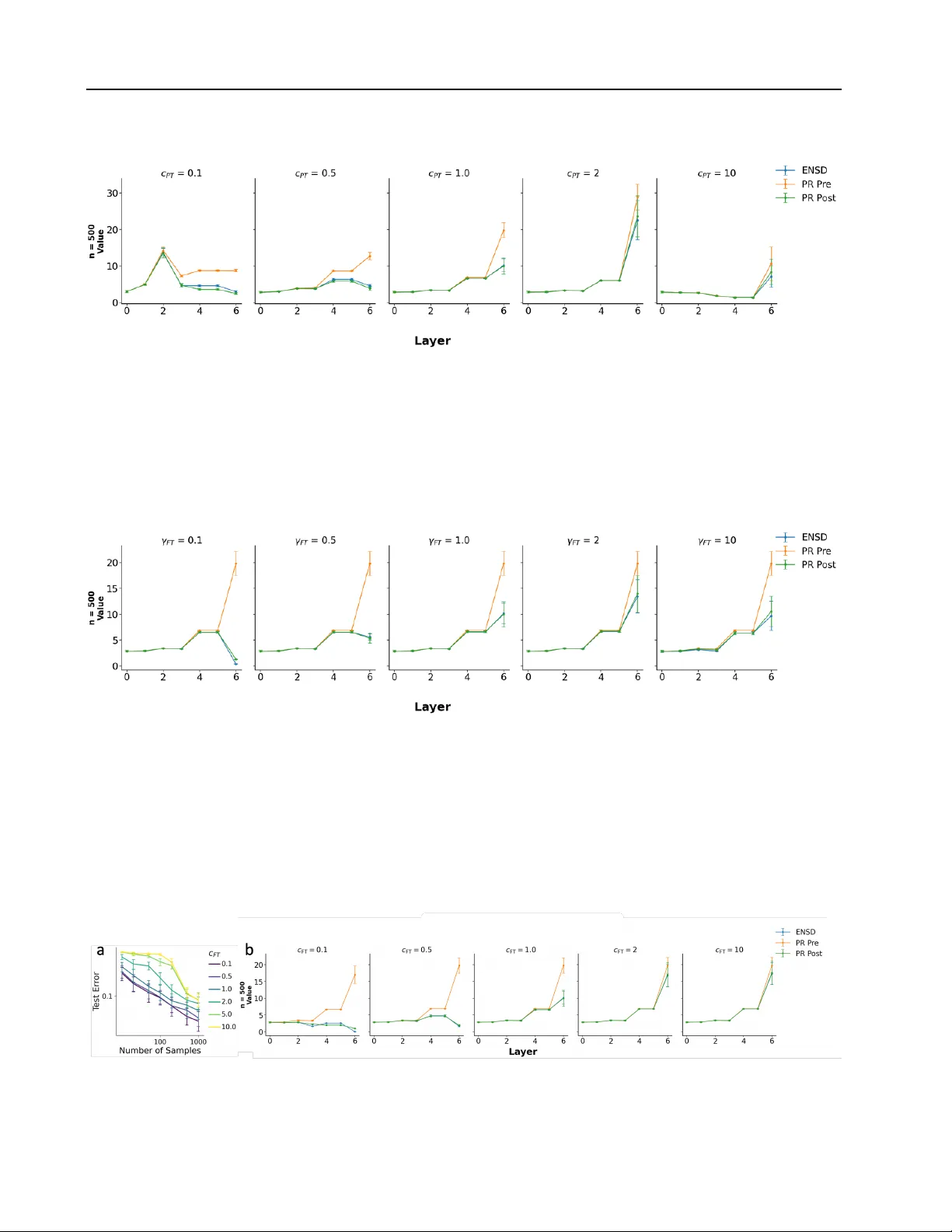
A Theory of How Pr etraining Shapes Inductiv e Bias in Fine-T uning Nicol ´ as Anguita 1 Francesco Locatello 2 Andrew M. Saxe 3 Marco Mondelli 2 Flavia Mancini 1 Samuel Lippl * 4 Cl ´ ementine Domin ´ e * 2 Abstract Pretraining and ﬁne-tuning are central stages in modern machine learning systems. In practice, feature learning plays an important role across both stages: deep neural networks learn a broad range of useful features during pretraining and further reﬁne those features during ﬁne-tuning. Ho wev er , an end-to-end theoretical understanding of how choices of initialization impact the ability to reuse and reﬁne features during ﬁne-tuning has remained elusiv e. Here we de velop an analytical theory of the pretraining–ﬁne-tuning pipeline in diagonal linear networks, deriving e xact expres- sions for the generalization error as a function of initialization parameters and task statistics. W e ﬁnd that dif ferent initialization choices place the network into four distinct ﬁne-tuning regimes that are distinguished by their ability to support fea- ture learning and reuse—and therefore by the task statistics for which the y are beneﬁcial. In partic- ular , a smaller initialization scale in earlier lay- ers enables the network to both reuse and reﬁne its features, leading to superior generalization on ﬁne-tuning tasks that rely on a subset of pretrain- ing features. W e demonstrate empirically that the same initialization parameters impact general- ization in nonlinear networks trained on CIF AR- 100. Overall, our results demonstrate analytically how data and network initialization interact to shape ﬁne-tuning generalization, highlighting an important role for the relativ e scale of initializa- tion across different layers in enabling continued feature learning during ﬁne-tuning. Co-senior authors (marked with *). 1 Department of Engineer - ing, University of Cambridge 2 Institute of Science and T echnol- ogy , Austria (IST A) 3 Gatsby Computational Neuroscience Unit and Sainsb ury W ellcome Centre, UCL 4 Center for Theoretical Neuroscience, Columbia Uni versity . Correspondence to: Nicol ´ as Anguita < na658@cam.ac.uk > . Pr eprint. F ebruary 24, 2026. 1. Introduction Deep neural networks are often trained in stages: ﬁrst, they are pretrained on general-purpose tasks for which large amounts of data are a vailable; then, they are ﬁne-tuned on the actual tar get task, for which data may be more limited. This pretraining–ﬁne-tuning pipeline (PT+FT) has emerged as an essential workhorse for modern deep learning ( Bom- masani , 2021 ; Parthasarath y et al. , 2024 ; A w ais et al. , 2025 ). T o beneﬁt from ﬁne-tuning, neural networks must learn task-speciﬁc features during pretraining and reuse them during ﬁne-tuning ( Lampinen & Ganguli , 2018 ; Saxe et al. , 2019 ; Shachaf et al. , 2021 ; T ahir et al. , 2024 ). At the same time, ﬁne-tuning further adapts these features, potentially improving generalization ( Y osinski et al. , 2014 ; Huh et al. , 2016 ; Jain et al. , 2023 ). As a result, the success of the PT+FT pipeline critically depends on ho w feature learning unfolds ov er the pretraining and ﬁne-tuning stages. Despite the practical success of PT+FT , the factors gov- erning feature learning across pretraining and ﬁne-tuning hav e remained unclear . Prior work has shown that weight initialization—in particular , its absolute and relati ve scale across layers—shifts neural network training between a ﬁxed-feature (“lazy”) and a feature-learning (“rich”) regime ( Chizat et al. , 2019 ; Braun et al. , 2022 ; Domin ´ e et al. , 2024 ; Kunin et al. , 2024 ). In the single-task setting, feature-learning regimes often induce improved generalization ( Chizat & Bach , 2020 ; F ort et al. , 2020 ; Vyas et al. , 2022 ). Ho we ver , it remains unclear how these insights extend to multi-stage training regimes such as PT+FT , with only a fe w exceptions discussed further in Section 2 ( Lippl & Lindsey , 2024 ). This limits our ability to use weight initialization as a principled tool for controlling the balance between reusing pretrained features and inducing continued feature learning. T o address this gap, we study the PT+FT pipeline in diagonal linear networks, a tractable theoretical model that exhibits feature-learning behavior , and dev elop an end-to-end theory of the resulting generalization error . Our theory elucidates ho w weight initialization af fects the inductiv e bias of PT+FT , and how this bias interacts with 1 data properties to determine when dif ferent initialization schemes are optimal. Speciﬁc Contributions. • W e analytically deriv e the implicit bias of PT+FT in diagonal linear networks and the resulting generaliza- tion error as a function of weight initialization, task parameters, and data scale (Section 4 ). • W e identify three limiting regimes induced by this im- plicit bias: (I) a pretraining-independent rich regime, (II) a pretraining-dependent lazy re gime, and (III) a pretraining-independent lazy regime. W e further high- light a uni versal trade-of f between pretraining depen- dence and feature learning in ﬁne-tuning (Section 5.1 ). • In light of this trade-of f, we highlight a fourth, interme- diate learning regime: (IV) the pretraining-dependent rich regime. Notably , we ﬁnd that the relativ e scale of initialization across layers plays a key role in entering this regime (Section 5.2 ). • W e demonstrate that pretraining and ﬁne-tuning task parameters determine which of these regimes will gen- eralize best (Section 5.3 ). • Finally , in Section 6 , we demonstrate that theoretical in- sights deri ved from simple networks extend to ResNets trained on CIF AR-100. Altogether , we provide an end-to-end understanding of how initialization choices shape ﬁne-tuning generalization. In doing so, we identify actionable lev ers for controlling the interplay between reusing pretrained features, reﬁning those features, and learning new features. 2. Related W ork Rich and Lazy Learning. The distinction between lazy and rich learning re gimes has become central to understanding ho w o verparameterized neural networks learn and generalize. In the lazy re gime, training dynamics are gov erned by a ﬁxed representation, causing the network to ef fectiv ely behave like a kernel machine ( Jacot et al. , 2018 ; Chizat et al. , 2019 ). In contrast, the rich (or feature-learning) regime is marked by the emergence of task-speciﬁc representations and is commonly linked to ﬁnite-width networks and smaller weight scales ( Saxe et al. , 2013 ; Chizat & Bach , 2020 ; Atanasov et al. , 2021 ). The rich regime is often deﬁned purely in distinction to the lazy regime; ho we ver , recent work has reﬁned this dichotomy by demonstrating that both the relative and absolute scale of initial weights across layers induce a continuum of feature-learning dynamics and corresponding inducti ve biases ( W oodworth et al. , 2020 ; Azulay et al. , 2021 ; Domin ´ e et al. , 2024 ; K unin et al. , 2024 ). Our work b uilds on these insights to show ho w this spectrum manifests in the PT+FT setting. W e show that, depending on task parameters, intermediate regimes can induce superior generalization, suggesting that analyses restricted to extreme cases may miss important behaviors. Implicit Regularization and Diagonal Linear Networks. Neural networks are often trained in an o verparameterized setting where there are many possible solutions to the training data. In this setting, the training procedure consistently biases the network to wards a particular solution (a phenomenon called “implicit bias”, Soudry et al. , 2018 ), explaining why neural networks generalize well e ven without explicit regularization ( Zhang et al. , 2016 ). Lazy and rich regimes often instantiate fundamentally distinct implicit biases. Lazy-re gime neural networks implement a kernel predictor , whereas rich-re gime neural networks are often biased towards learning lo w-dimensional or sparse representations ( Gunasekar et al. , 2018 ; Sav arese et al. , 2019 ; L yu & Li , 2019 ; Nacson et al. , 2019 ; Chizat & Bach , 2020 ). Diagonal linear netw orks (Section 3.1 ) instantiate a simple, analytically tractable model that captures the changes in inducti v e bias observed in more comple x models: lazy-regime training ﬁnds the (non-sparse) solution with minimal ℓ 2 -norm, whereas rich-regime training ﬁnds the sparse solution with minimal ℓ 1 -norm ( W oodworth et al. , 2020 ; Azulay et al. , 2021 ). Prior work has characterized the emergence of the inﬁnite-time solution in these networks ( Pesme & Flammarion , 2023 ; Berthier , 2023 ) and in vestigated the role of stochasticity and step size ( Pesme et al. , 2021 ; Nacson et al. , 2022 ). Implicit Regularization of Fine-T uning. In dense linear networks, a higher similarity in task features between pretraining and ﬁne-tuning generally impro ves generaliza- tion performance ( Lampinen & Ganguli , 2018 ; Shachaf et al. , 2021 ; T ahir et al. , 2024 ). Moreover , ﬁne-tuning with backpropagation can result in improved in-distribution generalization compared to only training the linear readout, but may harm out-of-distribution performance ( Kumar et al. , 2022 ; T omihari & Sato , 2024 ). These theories generally focus on single-output dense linear networks (which ha ve the same inductive bias in the rich and lazy regime) or training in the kernel regime ( Malladi et al. , 2023 ). In contrast, our perspectiv e allows us to characterize how different pretraining initializations shift the ﬁne-tuning behavior between the lazy and rich regime. Other works characterize the inﬂuence of pretraining data selection on ﬁne-tuning under distributional shifts ( Kang et al. , 2024 ; Cohen-W ang et al. , 2024 ; Jain et al. , 2025 ). Finally , Lippl & Lindsey ( 2024 ) characterized the inducti ve bias of 2 F igur e 1. Setup. Schematic illustration of the theoretical setup: dependence on the initialization parameters c P T , λ P T , and γ F T (shown in pink); and dependence on the data parameters ρ P T , ρ shared F T , and ρ new F T (shown in gre y). diagonal linear networks for inﬁnitesimal initial weights in pretraining and studied the resulting generalization behavior using simulations in a teacher -student setup. Here we substantially extend their work by characterizing the inducti ve bias conferred by a broad range of pretraining and ﬁne-tuning initializations, rev ealing a crucial role played by the relati ve scale of initialization. Moreover , we deriv e an analytical theory describing the generalization error (rather than relying on simulations), providing closer insight into speciﬁc conditions under which certain pretraining initializations help or hurt performance. Replica-theoretical Characterization of the Generaliza- tion Err or . W e le verage the replica method ( Edwards & Anderson , 1975 ; M ´ ezard et al. , 1987 ) to characterize the ability of diagonal linear networks to reco ver ground-truth parameters in a ﬁne-tuning setup. The replica method is non-rigorous, but provides a po werful tool for analytically characterizing estimation errors in the high-dimensional limit under dif ferent penalties, including ℓ 1 ( Guo & V erd ´ u , 2005 ; Rangan et al. , 2009 ). These formulas were later conﬁrmed using rigorous approaches ( Bayati & Montanari , 2011a ; b ). W e speciﬁcally rely on the approach in Bereyhi & M ¨ uller ( 2018 ); Bereyhi et al. ( 2019 ), which characterizes estimation errors with potentially different penalties across dimensions. Our results imply that pretraining can be understood as modifying the penalties across different dimensions; this is related to prior work on incorporating prior knowledge on the support in compressed sensing problems ( Khajehnejad et al. , 2009 ; V aswani & Lu , 2010 ). 3. Theoretical Setup 3.1. Network Ar chitecture W e study the generalization behavior of diagonal linear networks ( Fig. 1 ), a simple one-hidden-layer network archi- tecture that parametrizes linear maps f : R D → R as f w , v ( x ) = β ( w , v ) T x , (1) where β ( w , v ) := v + ◦ w + − v − ◦ w − ∈ R D ( ◦ indicates element-wise multiplication). Here, w + , w − ∈ R D com- prise the hidden weights of the network and v + , v − ∈ R D comprise its output weights. w + , v + and w − , v − param- eterize the positi ve and negati ve pathway , respecti vely; separating these pathways allo ws us to initialize the netw ork at β = 0 while a voiding a saddle point. Diagonal linear networks capture two key aspects of the deep neural networks used in practice: 1) their initial weights control their transition between the rich (feature- learning) and lazy (kernel) regime and 2) their generalization behavior is different between these regimes ( W oodworth et al. , 2020 ; Azulay et al. , 2021 ; Lippl & Lindse y , 2024 ). They therefore pro vide a useful theoretical model to study the impact of initialization on pretraining and ﬁne-tuning. 3.2. Network T raining W e in vestigate diagonal linear netw orks trained with gradient ﬂo w to minimize mean-squared error . W e consider two datasets: a pretraining (PT) task X P T ∈ R N P T × D , y P T ∈ R N P T and a ﬁne-tuning (FT) task X F T ∈ R N F T × D , y F T ∈ R N F T . The training proceeds in two stages: we ﬁrst pretrain on the PT task and then ﬁne-tune on the FT task (PT+FT). In both cases, we assume that the model trains to zero training error . W e denote the parameters learned during pretraining and ﬁne-tuning by w P T ( t ) , v P T ( t ) and w F T ( t ) , v F T ( t ) , the corresponding network functions by ˆ β P T ( t ) and ˆ β F T ( t ) , and their predictions by ˆ y P T = X P T ˆ β P T and ˆ y F T = X F T ˆ β F T . t denotes the learning time, t = 0 indicating the initial weights, and t = ∞ the weights at the end of training. Where the context is clear , we denote the network functions at the end of pretraining and ﬁne-tuning by ˆ β P T and ˆ β F T . Initialization. W e assume w + (0) = w − (0) and v + (0) = v − (0) (to av oid biasing the network towards positiv e or negati ve coefﬁcients). Building on insights from the fea- ture learning literature, we focus on two ke y aspects of the weight initialization: 1) the absolute scale (capturing the ov erall initial weight magnitude), c P T := w ± P T (0) 2 + v ± P T (0) 2 , (2) and 2) the relati ve scale (capturing the difference in initial weight magnitude between the ﬁrst and the second layer), λ P T := ( w ± P T (0) 2 − v ± P T (0) 2 ) /c P T ∈ [ − 1 , 1] . (3) 3 After pretraining, we re-balance the positiv e and negati ve pathways by setting w ± F T (0) := w + P T ( ∞ ) + w − P T ( ∞ ) , (4) to ensure that the ef fecti ve network function at the beginning of ﬁne-tuning is zero again: β F T (0) = 0 . Further, we re- initialize the readout weights to a ﬁxed scale γ F T ≥ 0 : v ± F T (0) := γ F T . (5) By systematically varying these three initialization parame- ters ( c P T , λ P T , and γ F T ), we aim to understand their ef fect on ﬁne-tuning performance. 3.3. Data Generative Model T o in vestigate the generalization performance of diago- nal linear networks trained in this manner, we consider a teacher -student setup , where we sample ground-truth pre- training and ﬁne-tuning functions (“teachers”) by sampling from a joint distribution β ∗ P T , β ∗ F T ∼ p P T ,F T ( β ∗ P T , β ∗ F T ) . W e generate the dataset by sampling random inputs, X P T , X F T ∼ N (0 , 1 D ) , and generating the outputs through the teachers, y P T = X P T β P T , y F T = X F T β F T . W e aim to characterize the de viation between the ground-truth β ∗ F T and the estimate resulting from ﬁne-tuning, ˆ β F T : E := ∥ β ∗ F T − ˆ β F T ∥ 2 2 . (6) W e characterize E through a replica-theoretical approach, which describes the network beha vior in the high- dimensional limit ( D → ∞ ), where we scale the pretraining and ﬁne-tuning data size with D : α P T := lim D →∞ N P T /D , α F T := lim D →∞ N F T /D . (7) W e will focus on the case α P T ≥ 1 , and as a result ˆ β P T = β ∗ P T is perfectly recov ered. W e call α F T (also known as the “load”) the data scale . Finally , we characterize a speciﬁc family of generati ve models p P T ,F T ( β ∗ P T , β ∗ F T ) , in which there are J underlying groups that are sampled with probabilities π ∈ R J for each dimension d ∈ { 1 , . . . , D } . For the sampled group j ∈ { 1 , . . . , J } , β ∗ P T ,d and β ∗ F T ,d are independently sampled from group-speciﬁc distributions p ( j ) P T and p ( j ) F T , i.e. their dependenc y is mediated via their group membership (see Deﬁnition C.1 ). T o in vestigate the consequences of our theory (and conﬁrm it in empirical simulations), we will focus on a spike-and- slab distrib ution for β ∗ P T , β ∗ F T . In diagonal linear networks, feature learning is useful when only a sparse subset of di- mensions are acti ve for a gi ven task. W e therefore sample the set of activ e dimensions for the pretraining task, θ P T ∼ Bernoulli ( ρ P T ) , θ P T ∈ { 0 , 1 } D , (8) and then generate β P T by sampling random signs for the activ e dimensions (i.e. any d for which θ d = 1 ): β P T = ( σ / √ ρ P T ) ◦ θ P T , σ ∼ Cat ( {− 1 , 1 } ) . (9) W e similarly assume that a subset of dimensions is acti ve on the ﬁne-tuning task by sampling θ F T ∈ { 0 , 1 } D . Ho wev er , in this case, whether a gi ven dimension is acti ve can depend on whether it was already acti ve on the pretraining task: θ F T | θ P T = 1 ∼ Bernoulli ( ρ shared F T /ρ P T ) , θ F T | θ P T = 0 ∼ Bernoulli ( ρ new F T / (1 − ρ P T )) , β F T = b F T ◦ θ F T , b F T ∼ N (0 , 1 ρ shared F T + ρ new F T ) . (10) Thus, ρ shared F T ≥ ρ new F T means that dimensions active during pretraining are more likely to be acti ve during ﬁne-tuning, whereas ρ shared F T ≤ ρ new F T means that they are less likely . Fig. 1 depicts the network conﬁguration varying the task parameters. T aken together , we will characterize ho w 1) initialization parameters, c P T , λ P T , and γ F T , 2) task parameters, ρ P T , ρ shared F T , and ρ new F T , and 3) data scale, α F T , impact generaliza- tion during ﬁne-tuning. 4. Theoretical Characterization of Generalization Error in Fine-T uning W e will deriv e a theoretical characterization of the gen- eralization error E in two steps: ﬁrst, we will deriv e the implicit regularization induced by PT+FT in diagonal linear networks as a function of initialization parameters (Theo- rem 4.1 ), then we will characterize the generalization error induced by the different possible regularization penalties for our data generativ e model (Proposition 4.2 ). 4.1. Implicit Inductive Bias of Fine-T uning W e ﬁrst deri ve the implicit inducti ve bias of ov erparam- eterized diagonal networks under the ﬁne-tuning training paradigm, building on analysis in prior work ( Azulay et al. , 2021 ; Lippl & Lindsey , 2024 ). Theorem 4.1 (Implicit bias) . Consider a diagonal lin- ear network trained under the paradigm described in Sec- tion 3.2 . Then, the gr adient ﬂow solution at con ver gence is 4 given by arg min β F T Q k ( β F T ) s.t. X ⊤ F T β F T = y F T , (11) wher e Q k ( β F T ) = D X d =1 q k d ( β F T ,d ) , (12) q k ( z ) = √ k 4 1 − r 1 + 4 z 2 k + 2 z √ k arcsinh  2 z √ k  ! , (13) k d =  2 c P T (1 + λ PT )  1 + q 1 + ( ˆ β PT , d /c PT ) 2  + γ 2  2 . (14) Pr oof. Azulay et al. ( 2021 ) proved that c P T (when deﬁned as c P T = w + w − + v + v − ) and λ P T are conserv ed through- out training (see also Marcotte et al. , 2023 ). Extended cal- culations allow us to reco ver the indi vidual layers’ weights from the effecti ve network weights after pretraining. Details are relegated to Appendix B.1 due to space constraints. Theorem 4.1 sho ws that the function selected by the network depends on λ P T , c P T , and γ F T in a non-tri vial manner . Im- portantly , this implicit bias also depends on ˆ β P T , implying that the learned solution potentially depends on the pretrain- ing task. Notably , e ven though in diagonal linear networks, the relative scale λ P T does not impact the inducti ve bias of pretraining, it does impact the learned hidden represen- tation and therefore the inductive bias of ﬁne-tuning. In Section 5.1 we sho w how these dependencies shape the re- sulting learning regime. This substantially extends results by Lippl & Lindsey ( 2024 ), which focused on c P T → 0 with λ PT = 0 , γ F T = 0 . W e will sho w that this only captures a subset of the range of learning regimes we identify . In particular , and perhaps surprisingly , we will see that ev en for very small c P T , dif ferent values for λ P T can fundamentally change the generalization behavior . 4.2. Replica Theory of the Generalization Error In practice, this implicit bias manifests in the sample ef- ﬁciency and generalization performance observ ed during ﬁne-tuning. T o understand the impact of the implicit bias deriv ed in Theorem 4.1 on generalization, we now turn to solving the corresponding optimization problem. ˆ β := arg min β ∈ R D 1 2 λ ∥ X F T β − y F T ∥ 2 2 + Q k ( β F T ) , β ∈ R D , k ∈ R D + . (15) For λ → 0 , this precisely characterizes the implicit induc- ti ve bias of a diagonal linear network trained on the training data ( X F T , y F T ) . W e aim to characterize how accurately this optimization problem can recover the ground-truth v ec- tor β ∗ F T ∈ R D , giv en the label y F T = X F T β ∗ F T + ε, ε ∼ N (0 , σ 2 0 ) . (16) Note that while our theory also applies to σ 2 0 > 0 , we will focus on the noiseless case σ 2 0 = 0 . W e assume that β ∗ F T , β ∗ P T are sampled from the joint distribution described abov e. This connects our setting to the setting studied in Bereyhi & M ¨ uller ( 2018 ), allowing us to characterize the generalization error in the high-dimensional limit. Proposition 4.2. Let N F T → ∞ and N F T /D → α F T > 0 . Then, under the r eplica assumption, the estimation pr ob- lem ( 15 ) decouples into a scalar pr oblem ˆ β sc ( y ; k , θ ) := arg min β ∈ R  ( y − β ) 2 2 θ + Q k ( β )  . (17) Speciﬁcally , ( β ∗ d , ˆ β d , k d ) con ver ge in distrib ution to ˆ β d = ˆ β sc ( β ∗ d + η ; k d , θ ) , η ∼ N (0 , θ 0 ) . (18) Her e θ and θ 0 ar e the “effective” r egularization and noise parameters. The y are not only governed by the external noise and r e gularization, but also by the noise and r e gular - ization induced fr om estimating the other parameters. These two pr operties ar e governed by the ﬁxed-point equations p = J X j =1 π j E β ∗ ,k,η h ( ˆ β sc ( β ∗ + η ; k , θ ) − β ∗ ) 2 i , (19) χ = θ J X j =1 π j E β ∗ ,k,η h ∂ y ˆ β sc ( β ∗ + η ; k , θ ) i , (20) wher e θ = λ + χ α , θ 0 = σ 2 0 + p α . Pr oof. The proposition follo ws from Proposition 1 in Bereyhi & M ¨ uller ( 2018 ), see Appendix C . This proposition, paired with Theorem 4.1 , yields an e xact formula for the generalization error associated with PT+FT in diagonal linear networks, as a function of weight initial- ization, task parameters, and data scale. 5. Understanding Learning Regimes in PT+FT The theoretical insights de veloped in Section 4 help us understand the inductiv e bias of PT+FT across the full spectrum of weight initialization and task parameters. W e ﬁrst use Theorem 4.1 to characterize ho w the initialization parameters inﬂuence the network’ s learning regime (Sec- tions 5.1 and 5.2 ) and then use Proposition 4.2 to tie these different learning regimes to the task parameters for which they are fa vorable (Section 5.3 ). 5 5.1. Learning Regimes in the Limit Building on Theorem 4.1 , we characterize the learning regime of the networks using two measures (introduced in Lippl & Lindsey ( 2024 )): 1. The ℓ -order := ∂ log q k d ( β F T ,d ) ∂ log | β F T ,d | , measures whether the network beneﬁts from sparsity . ℓ -order = 1 indicates a sparse inductiv e bias (e.g. the ℓ 1 -norm), whereas ℓ -order = 2 corresponds to a non-sparse inducti ve bias (e.g. the ℓ 2 -norm). 2. The pretraining dependence 1 , PD := ∂ log q k d ( β F T ,d ) ∂ log | β P T ,d | measures whether the network beneﬁts from pretrained features. PD = − 1 indicates that the penalty is in- versely proportional to the magnitude of the pretrained feature | β P T ,d | , whereas PD = 0 indicates that the penalty does not depend on it at all. While the ℓ -order arises as a rele vant quantity in single-task learning as well, PD only arises in a multi-task setting. W e deri ve analytical formulas for these metrics as a function of both the initialization parameters and β P T ,d and β F T ,d (see Appendix B.2 ). W e further identify a univ ersal tension between ℓ -order and PD: Proposition 5.1. W e identify the following ranges across the full spectrum of initialization: ℓ -or der ∈ [1 , 2] , PD ∈ [ − 1 , 0] , ℓ -or der + PD ∈ [1 , 2] . Pr oof. W e deriv e these ranges in Appendix B.2 . They e x- tend a ﬁnding from Lippl & Lindsey ( 2024 ) who found that ℓ -order + PD = 1 for c P T → 0 , λ P T , γ F T = 0 . In Fig. 2 a , we identify three limiting regimes arising from the interplay between the ℓ -order and pretraining depen- dence. T aking appropriate limits of the initialization param- eters λ P T and c P T places the model in these regimes, each corresponding to familiar norm-based regularization: (I) A rich, pretraining-independent regime , (ne w di- mensions learned; ℓ -order = 1, PD = 0). This regime is gov erned by the ℓ 1 -norm: Q ( β F T ) → ∥ β F T ∥ 1 and is induced, for instance, in the limit λ P T → − 1 , γ F T → 0 . W e call an ℓ 1 -like inducti ve bias in diagonal linear networks “rich”, because it arises from the feature- learning dynamics (see Section 2 ). (II) A lazy , pretraining-dependent regime , (reuse with minimal adaptation; ℓ -order = 2, PD = -1). This re gime is governed by the weighted ℓ 2 -norm: Q ( β F T ) → 1 Lippl & Lindsey ( 2024 ) introduced this metric as feature dependence; we call it pretraining dependence to emphasize that it characterizes the dependence on the pretraining function directly . b Active dimensions Inactive dimensions 1 2 l- or der -1 0 P r etraining dependence rich, pretraining- independent rich, pretraining- dependent lazy , pretraining- independent lazy , pretraining- dependent I II III IV Decr easing λ PT for pr etrained featur es Incr easing c PT / γ F T for pr etrained featur es Incr easing c PT / γ F T for non-pr etrained featur es a 10 3 5 10 c PT 1 0 1 PT PT, d = FT, d 10 3 5 10 c PT 1 0 1 PT PT, d = 0 10 3 5 10 FT 1 0 1 PT 10 3 5 10 FT 1 0 1 PT F igur e 2. Implicit bias and learning r egimes of ﬁne-tuning. (a) ℓ -order and pretraining dependence jointly deﬁne four different learning regimes in PT+FT . Different initialization parameters induce changes between these learning regimes, as indicated by the arrows. (b) W e can interpolate between these four regimes (for a color legend, see panel (a)) by shifting the initialization parameters ( ˆ β F T ,d = 1 / √ ρ F T , ρ F T = 0 . 1 ). Crucial transitions, which we further highlight in the text and in panel (a), are indicated by the arrows. Simulation details can be found in Appendix E . P D i =1 | β F T ,i | 2 / | β P T ,i | . This regime is induced, for instance, by considering c P T → 0 and λ P T → 1 . (III) A lazy , pretraining-independent r egime ( ℓ -order = 2, PD = 0). This regime is governed by the unweighted ℓ 2 - norm: Q ( β F T ) → ∥ β F T ∥ 2 and implies that the ﬁne- tuning behavior does not depend on the pretraining task at all. This re gime is induced, for instance, by taking c P T → ∞ or γ F T → ∞ . W e highlight the identiﬁcation of a nov el regime—the lazy , pr etraining-independent r e gime —which goes beyond pre vi- ous works. This re gime is accessible only in the ﬁne-tuning setting and highlights that for badly chosen initialization parameters, pretraining will not create transferable features. 5.2. Full Phase Portrait of the Lear ning Regimes In Section 5.1 , our analysis was restricted to asymptotic behavior . Howe ver , in practice we may be operating in an intermediate learning regime where the parameters do not approach one of the above limits. Indeed, operating in such a regime will often confer a beneﬁcial inductive bias: On the one hand, for pretraining to be useful, the penalty should depend on the active pretraining dimensions, i.e. ideally PD = − 1 . On the other hand, a sparse inductiv e bias substantially improv es generalization performance (if the ground truth is also sparse), i.e. ideally ℓ -order = 1 . Proposition 5.1 highlights a fundamental tradeof f between these desiderata: it is impossible to achiev e PD = − 1 and ℓ -order = 1 . The set of possible v alues for the pair ( ℓ -order , P D ) is giv en by a triangle whose edges are giv en by regimes (I-III) ( Fig. 2 b ). W e thus highlight an important intermediate regime: (IV) The pretraining-dependent rich regime ( ℓ -order < 6 2 , P D < 0 ) achieves a balance between pretraining dependence and ℓ -order , enabling the model to leverage both sparsity and feature reuse simultaneously . Overall, the four learning regimes we highlight are distin- guished by their pretraining dependence and sparsity bias/ ℓ - order . T o understand ho w the initialization parameters im- pact the learning regime, we plot the full phase portrait of the learning re gimes as a function of pretraining initial- ization ( Fig. 2 b ), considering a typical v alue at the end of training, β F T ,d = 1 / √ ρ F T (setting ρ F T = 0 . 1 as this will be a common task setting in the subsequent section). W e note that because of our task generation process, we either hav e β ∗ P T ,d = ± 1 / √ ρ P T (setting ρ P T = 0 . 1 as well) or β ∗ P T ,d = 0 . W e therefore plot the phase diagram for both cases, which clariﬁes which learning regime we operate in for acti ve dimensions ( β ∗ P T ,d = ± 1 / √ ρ P T ) and inactiv e dimensions ( β ∗ P T ,d = 0 ). For activ e dimensions where β ∗ P T ,d = ± 1 / √ ρ P T , changing the relativ e scale λ P T shifts the network from the lazy , pr etr aining-dependent r e gime (II) to the rich, pr etraining-independent re gime (I), with intermediate scales yielding the rich, pr etr aining-dependent re gime (IV) (see the dotted line in Fig. 2 a,b ). Intuiti vely , a negati ve λ P T implies that the second-layer weights dominate over the ﬁrst layer ( v > w ), while a positiv e λ P T indicates the opposite ( w > v ). When λ P T is large and negativ e, the ﬁrst-layer representation is comparativ ely small, ev en after pretraining. After rescaling the second layer to γ F T = 0 , these lar ge second-layer weights are reduced, decreasing the ov erall scale of the network—this driv es the system tow ard the rich regime. In contrast, as λ P T increases, the learned ﬁrst-layer representation becomes larger , driving the network into the lazy , pr etraining-dependent r e gime . In contrast, increasing the absolute scale c P T or the ﬁne-tuning re-initialization scale γ F T mov es the system toward the lazy pr etraining-independent re gime (III), where neither sparsity nor shared dimensions improve generalization (solid line in Fig. 2 a,b ). For inacti ve dimensions ( β ∗ P T ,d = 0 ), we ﬁnd that PD = 0 . Thus, instead of the two-dimensional continuum outlined abov e, we recover a one-dimensional continuum between the lazy pretr aining-independent r e gime (III) and the rich pr etraining-independent r e gime (I) ( Fig. 2 b , right column). Increasing γ F T or c P T shifts the inductiv e bias from re gime (I) into regime (III) (see the dashed line in Fig. 2 a,b ). Additionally , (albeit less pronounced), increasing λ P T also shifts the inductiv e bias into a slightly lazier regime. Overall, the dif ferent initialization parameters can therefore change the inducti ve bias of PT+FT along three ax es: they can control 1) whether the network beneﬁts from shared dimensions with the pretraining task (measured by the PD for active dimensions), 2) whether the network beneﬁts from sparsity in the new activ e dimensions (measured by the ℓ -order for β ∗ P T ,d = 0 ), and 3) whether the network beneﬁts from sparsity in the shared active dimensions (mea- sured by the ℓ -order for active dimensions). In the next section, we le verage Proposition 4.2 to sho w that this allows us to understand ho w these dif ferent initializations impact generalization performance across task parameters. 5.3. Learning Regime and T ask Parameters Jointly Determine Generalization Error Cur ves In practice, the implicit bias described abov e is reﬂected in the sample efﬁciency and generalization performance observed during ﬁne-tuning. W e solve the ﬁxed-point equa- tions deri ved in Proposition 4.2 to understand ho w the dif- ferent learning regimes and task parameters impact general- ization performance. In particular, we examine the impact of the different initialization parameters on the three axes outlined abov e. W e additionally directly train diagonal lin- ear netw orks in a PT+FT setup to validate our analytical characterization with empirical simulations. Do we beneﬁt fr om shar ed dimensions? If our penalty implements pretraining dependence, we should beneﬁt from sharing dimensions between pretraining and ﬁne-tuning. W e therefore consider a ﬁx ed ρ P T = 0 . 1 and compare the case ρ shared F T = 0 . 1 , ρ new F T = 0 (in which case the pretraining and ﬁne-tuning task share all their dimensions) to the case ρ shared F T = 0 , ρ new F T = 0 . 1 (in which case they share no dimen- sions, but the overall sparsity le vel is matched). As c P T and γ F T decrease, performance becomes increasingly sensitiv e to task overlap ( Fig . 3 a,b ). On the other hand, decreasing λ P T decreases the extent to which we beneﬁt from shared dimensions ( Fig. 3 c ). These trends are consistent with the phase-portrait analysis, which indicates that for pretrained dimensions, decreasing γ F T and c P T at ﬁx ed λ P T shifts the network from a lazy , pr etraining-independent r egime tow ard a lazy , pr etraining-dependent r e gime (solid line in Fig. 2 ). In contrast, decreasing λ P T shifts the model from a lazy , pr etraining-dependent re gime to a rich, pr etraining-independent r e gime (dotted line in Fig. 2 ). Do we beneﬁt from sparsity in new activ e dimensions? For inactiv e dimensions (i.e. β ∗ P T ,d = 0 ), we can either be in a rich regime where we beneﬁt from a sparse set of ne w dimensions, or a lazy re gime where we learn sparse and non-sparse sets equally well. W e therefore consider a task with no shared dimensions with the pretraining task ( ρ P T = 0 . 1 , ρ shared F T = 0 ) and compare performance across dif ferent le vels of sparsity on the 7 F igur e 3. Generalization curves for differ ent initialization parameters and task parameters. The generalization error E as a function of the data scale α F T . Lines depict replica predictions and points depict the results of our empirical simulations ( ± 2 standard errors). In all cases, ρ P T = 0 . 1 . W e consider c P T = 10 − 3 , λ P T = 0 , and γ F T = 0 , v arying one initialization parameter for each panel. Simulation details can be found in Appendix E . (a-c) W e consider either o verlapping ( ρ shared F T = 0 . 1 , ρ new F T = 0 ) or distinct ( ρ shared F T = 0 , ρ new F T = 0 . 1 ) FT dimensions. (d,e) W e consider ρ shared F T = 0 and vary ρ new F T . (f) W e consider ρ new F T = 0 and vary ρ shared F T . ﬁne-tuning task ( ρ F T = 0 . 1 , 0 . 9 ). W e observe that as c P T and γ F T decrease, sparsity becomes increasingly beneﬁcial for performance ( Fig. 3 d,e ). This observ ation aligns with the phase-portrait analysis, which sho ws that for β ∗ P T ,d = 0 the model undergoes a transition from a lazy , pr etraining-independent r e gime , which has no sparsity bias, to a rich, pr etraining-independent r e gime that supports the learning of ne w , useful dimensions and has a sparsity bias (dashed line in Fig. 2 ). Do we beneﬁt fr om sparsity in shared active dimensions? Rich learning regimes should also beneﬁt from sparsity in pretrained dimensions (with β ∗ P T ,d = ± 1 / √ ρ P T ). W e therefore consider fully ov erlapping dimensions ( ρ P T = 0 . 1 , ρ new F T = 0 ) and compare ρ shared F T = 0 . 1 to ρ shared F T = 0 . 01 . W e observe that as λ P T decreases, the network increasingly beneﬁts from sparsity ( Fig. 3 f ). Howe ver , this ef fect vanishes if c P T or γ F T are very large. This observation again aligns with the phase-portrait analysis: as λ P T decreases, we move into the rich, pr etraining-dependent r e gime (dotted line in Fig . 2 ), but if c P T or γ F T increase, we move into the lazy , pr etraining- independent r e gime regardless of λ P T . T aken together , the generalization curves elucidate ho w ini- tialization parameters interact with task parameters to shape generalization behavior . In particular, the generalization curves demonstrate the same trade-of f between sparsity and pretraining dependence we predicted from Proposition 5.1 : as λ P T becomes more negativ e, we move along the diagonal representing the trade-of f between ℓ -order and pretraining dependence (dotted line in Fig. 2 ) . As a result, the network beneﬁts less from overlap: for ρ shared F T = 0 . 1 (indicating a full ov erlap between pretrained and ﬁne-tuned dimensions), decreasing λ P T makes generalization worse ( Fig. 3 f ). At the same time, the network beneﬁts more from sparsity: for ρ shared F T = 0 . 01 , trading of f a stronger sparsity bias for a weaker pretraining dependence is worthwhile, and a smaller λ P T yields better performance. Overall, this identiﬁes λ P T as a crucial factor for changing the inducti ve bias of PT+FT and highlights that the optimal learning regime will depend on the task parameters (see Fig. 5 in the Appendix). F igur e 4. ResNet CIF AR-100. Generalization performance as a function of the number of samples and initialization parameters. W e vary (a) the absolute scale of initialization by multiplying all weights in the network by c P T , (b) the relative scale of initial- ization by multiplying the ﬁrst three blocks of the ResNet by κ (equiv alent to λ P T ), and (c) the readout initialization by multiply- ing the readout by γ F T (Simulation details: Appendix E ). 6. Large-Scale V ision Experiments Our theoretical analysis and small-scale experiments suggest that modifying pretraining parameters and rescaling parameters provides a theoretically principled mechanism for inducing useful feature learning during ﬁne-tuning. T o ev aluate this prediction, we pretrain a ResNet on 98 classes from CIF AR-100 and subsequently ﬁne-tune it on the remaining two classes. The class split is sampled randomly and repeated ﬁfty times. W e design three experimental settings that translate the theoretical parameters λ P T , c P T , and γ F T to a realistic deep-network architecture. The ResNet-18 architecture consists of an initial embedding layer followed by four stages of residual blocks, each containing two con volutional layers with identity skip connections. T o induce imbalance across network layers, we upscale the embedding layer and the ﬁrst three residual stages by a constant factor κ . T o implement an equi v alent notion of c P T scaling in this architecture, we scale all 8 network parameters by a constant factor . Finally , to implement an analogue of γ F T , we rescale the parameters of the ﬁnal classiﬁcation layer after pretraining 2 Further experimental details are pro vided in Appendix D . In Fig. 4 a , we observ e that a ResNet initialized with a non- standard small v alue of κ —where κ < 1 corresponds to a negati ve relati ve scaling—exhibits improv ed generaliza- tion during ﬁne-tuning. Similarly , as sho wn in Fig . 4 b , in- creasing the scale of c P T also leads to degraded ﬁne-tuning generalization, in agreement with our theoretical predic- tions. Finally , Fig. 4 c sho ws that decreasing the scale of γ F T improv es ﬁne-tuning generalization for intermediate sample sizes. In Appendix D , we provide a representation- lev el analysis of the three settings, ﬁnding that all three settings induce a ke y representational signature indicativ e of the pr etraining-dependent rich re gime . All parameters identiﬁed by the theory have a meaningful impact on gen- eralization during ﬁne-tuning in practice. Ho wev er , these results should be interpreted with caution when e xtrapolat- ing to lar ge-scale architectures, as se veral ke y dif ferences, including depth and nonlinearities, may affect their applica- bility (discussed in Appendix D ). 7. Conclusion Despite the prev alence of the pretraining–ﬁne-tuning (PT+FT) pipeline in modern deep learning, a comprehensi ve understanding of the inductive bias of PT+FT , and how it relates to initialization structure and task parameters, has remained elusiv e. Here we de veloped an end-to-end theory of PT+FT in diagonal linear networks, analytically comput- ing the generalization error as a function of initialization parameters, task parameters, and data scale. Albeit based on a simpliﬁed neural network model, our analysis pro- vides quantitativ e insights relev ant to practical scenarios in machine learning and neuroscience. In particular, it under - scores the importance of relative weight scales across layers. Extending this framew ork to nonlinear networks represents an important next step. Finally , measuring the ℓ -order and pretraining dependence in more comple x architectures—e.g. using inﬂuence functions ( K oh & Liang , 2017 )—could help uncov er ho w feature reuse and adaptation arise during learn- ing across both artiﬁcial and biological systems. Impact Statement This paper presents work whose goal is to advance the ﬁeld of Machine Learning. There are many potential societal consequences of our work, none of which we feel must be speciﬁcally highlighted here. 2 For completeness, we report in Appendix D the heuristic proposed by Lippl & Lindsey ( 2024 ). Acknowledgements N A thanks the Rafael del Pino Foundation for ﬁnancial support. This research was funded in whole or in part by the Austrian Science Fund (FWF) 10.55776/COE12. SL acknowledges support by NSF 1707398 (Neuronex) and Gatsby Charitable F oundation GA T3708. This work was supported by a Schmidt Science Polymath A ward to AS, and the Sainsbury W ellcome Centre Core Grant from W ellcome (219627/Z/19/Z) and the Gatsby Charitable Foundation (GA T3850). FM is funded by a MRC Career Dev elopment A ward (MR/T010614/1), a UKRI Advanced Pain Discov- ery Platform grant (MR/W027593/1), and a EPSRC/MRC Programme Grant (UKRI1970). For the purpose of open access, the authors hav e applied a CC BY public copyright license to any Author Accepted Manuscript version arising from this submission. References Atanasov , A., Bordelon, B., and Pehlev an, C. Neural net- works as kernel learners: The silent alignment effect, 10 2021. URL https://openreview.net/forum? id=1NvflqAdoom . A wais, M., Naseer , M., Khan, S., Anwer, R. M., Cholakkal, H., Shah, M., Y ang, M.-H., and Khan, F . S. Foundation models deﬁning a ne w era in vision: a surve y and outlook. IEEE T ransactions on P attern Analysis and Machine In- telligence , 2025. Azulay , S., Moroshk o, E., Nacson, M. S., W oodworth, B. E., Srebro, N., Globerson, A., and Soudry , D. On the im- plicit bias of initialization shape: Beyond inﬁnitesimal mirror descent. In International Confer ence on Machine Learning , pp. 468–477. PMLR, 2021. Bayati, M. and Montanari, A. The dynamics of message passing on dense graphs, with applications to compressed sensing. IEEE T ransactions on Information Theory , 57 (2):764–785, 2011a. Bayati, M. and Montanari, A. The lasso risk for gaussian matrices. IEEE T ransactions on Information Theory , 58 (4):1997–2017, 2011b. Bereyhi, A. and M ¨ uller , R. R. Maximum-a-posteriori signal recov ery with prior information: Applications to com- pressi ve sensing. In 2018 IEEE International Confer ence on Acoustics, Speech and Signal Processing (ICASSP) , pp. 4494–4498. IEEE, 2018. Bereyhi, A., M ¨ uller , R. R., and Schulz-Baldes, H. Statistical mechanics of map estimation: General replica ansatz. IEEE T ransactions on Information Theory , 65(12):7896– 7934, 2019. 9 Berthier , R. Incremental learning in diagonal linear net- works. Journal of Machine Learning Resear ch , 24(171): 1–26, 2023. Bommasani, R. On the opportunities and risks of foundation models. arXiv pr eprint arXiv:2108.07258 , 2021. Braun, L., Domin ´ e, C., Fitzgerald, J., and Saxe, A. Exact learning dynamics of deep linear networks with prior knowledge. Advances in Neural Information Pr ocessing Systems , 35:6615–6629, 12 2022. Chizat, L. and Bach, F . Implicit bias of gradient descent for wide two-layer neural networks trained with the logistic loss. In Confer ence on learning theory , pp. 1305–1338. PMLR, 2020. Chizat, L., Oyallon, E., and Bach, F . On lazy training in dif ferentiable programming. Advances in neural informa- tion pr ocessing systems , 32, 2019. Cohen-W ang, B., V endrow , J., and Madry , A. Ask your distribution shift if pre-training is right for you. arXiv pr eprint arXiv:2403.00194 , 2024. Domin ´ e, C. C., Anguita, N., Proca, A. M., Braun, L., Kunin, D., Mediano, P . A., and Saxe, A. M. From lazy to rich: Exact learning dynamics in deep linear networks. arXiv pr eprint arXiv:2409.14623 , 2024. Edwards, S. F . and Anderson, P . W . Theory of spin glasses. Journal of Physics F: Metal Physics , 5(5):965, 1975. Fort, S., Dziugaite, G. K., Paul, M., Kharaghani, S., Ro y , D. M., and Ganguli, S. Deep learning versus kernel learning: an empirical study of loss landscape geome- try and the time e volution of the neural tangent kernel. Advances in Neural Information Pr ocessing Systems , 33: 5850–5861, 2020. Gao, P ., Trautmann, E., Y u, B., Santhanam, G., Ryu, S., Shenoy , K., and Ganguli, S. A theory of multineuronal dimensionality , dynamics and measurement. BioRxiv , pp. 214262, 2017. Giaff ar , H., Bux ´ o, C. R., and Aoi, M. The effecti ve number of shared dimensions between paired datasets. In Interna- tional Confer ence on Artiﬁcial Intelligence and Statistics , pp. 4249–4257. PMLR, 2024. Gunasekar , S., Lee, J., Soudry , D., and Srebro, N. Charac- terizing implicit bias in terms of optimization geometry . In International Conference on Machine Learning , pp. 1832–1841. PMLR, 2018. Guo, D. and V erd ´ u, S. Randomly spread cdma: Asymptotics via statistical physics. IEEE T ransactions on Information Theory , 51(6):1983–2010, 2005. Huh, M., Agraw al, P ., and Efros, A. A. What makes imagenet good for transfer learning? arXiv preprint arXiv:1608.08614 , 2016. Jacot, A., Gabriel, F ., and Hongler , C. Neural tangent ker- nel: Con vergence and generalization in neural networks. Advances in neural information pr ocessing systems , 31, 2018. Jain, A., Montanari, A., and Sasoglu, E. T rain on V alidation (T oV): Fast data selection with applications to ﬁne-tuning. arXiv pr eprint arXiv:2510.00386 , 2025. Jain, S., Kirk, R., Lubana, E. S., Dick, R. P ., T anaka, H., Grefenstette, E., Rockt ¨ aschel, T ., and Krueger , D. S. Mechanistically analyzing the effects of ﬁne- tuning on procedurally deﬁned tasks. arXiv preprint arXiv:2311.12786 , 2023. Kang, F ., Just, H. A., Sun, Y ., Jahagirdar , H., Zhang, Y ., Du, R., Sahu, A. K., and Jia, R. Get more for less: Principled data selection for warming up ﬁne-tuning in llms. arXiv pr eprint arXiv:2405.02774 , 2024. Khajehnejad, M. A., Xu, W ., A vestimehr , A. S., and Hassibi, B. W eighted ℓ 1 minimization for sparse reco very with prior information. In 2009 IEEE international symposium on information theory , pp. 483–487. IEEE, 2009. K oh, P . W . and Liang, P . Understanding black-box predic- tions via inﬂuence functions. In International conference on machine learning , pp. 1885–1894. PMLR, 2017. Kumar , A., Raghunathan, A., Jones, R., Ma, T ., and Liang, P . Fine-tuning can distort pretrained features and underperform out-of-distribution. arXiv preprint arXiv:2202.10054 , 2022. Kunin, D., Ravent ´ os, A., Domin ´ e, C., Chen, F ., Klindt, D., Saxe, A., and Ganguli, S. Get rich quick: ex- act solutions rev eal how unbalanced initializations pro- mote rapid feature learning, 06 2024. URL https: //arxiv.org/abs/2406.06158 . Lampinen, A. K. and Ganguli, S. An analytic theory of generalization dynamics and transfer learning in deep linear networks. arXiv pr eprint arXiv:1809.10374 , 2018. Lippl, S. and Lindsey , J. Inducti ve biases of multi-task learn- ing and ﬁnetuning: multiple re gimes of feature reuse. In The Thirty-eighth Annual Confer ence on Neural Informa- tion Pr ocessing Systems , 2024. L yu, K. and Li, J. Gradient descent maximizes the mar- gin of homogeneous neural networks. arXiv preprint arXiv:1906.05890 , 2019. 10 Malladi, S., W ettig, A., Y u, D., Chen, D., and Arora, S. A kernel-based vie w of language model ﬁne-tuning. In In- ternational Confer ence on Machine Learning , pp. 23610– 23641. PMLR, 2023. Marcotte, S., Gribon val, R., and Peyr ´ e, G. Abide by the law and follo w the ﬂow: conservation laws for gradient ﬂo ws, 12 2023. URL https://proceedings.neurips. cc/paper_files/paper/2023/hash/ c7bee9b76be21146fd592fc2b46614d5- Abstract- Conference. html . M ´ ezard, M., Parisi, G., and V irasoro, M. A. Spin glass the- ory and be yond: An Intr oduction to the Replica Method and Its Applications , volume 9. W orld Scientiﬁc Publish- ing Company , 1987. M ¨ uller , R. R., Alfano, G., Zaidel, B. M., and de Miguel, R. Applications of large random matrices in communications engineering. arXiv pr eprint arXiv:1310.5479 , 2013. Nacson, M. S., Gunasekar , S., Lee, J., Srebro, N., and Soudry , D. Lexicographic and depth-sensitiv e margins in homogeneous and non-homogeneous deep models. In International Confer ence on Machine Learning , pp. 4683– 4692. PMLR, 2019. Nacson, M. S., Ravichandran, K., Srebro, N., and Soudry , D. Implicit bias of the step size in linear diagonal neu- ral networks. In International Conference on Machine Learning , pp. 16270–16295. PMLR, 2022. Parthasarathy , V . B., Zafar , A., Khan, A., and Shahid, A. The ultimate guide to ﬁne-tuning llms from basics to breakthroughs: An exhausti ve review of technologies, research, best practices, applied research challenges and opportunities. arXiv pr eprint arXiv:2408.13296 , 2024. Pesme, S. and Flammarion, N. Saddle-to-saddle dynamics in diagonal linear networks. Advances in Neur al Informa- tion Pr ocessing Systems , 36:7475–7505, 2023. Pesme, S., Pillaud-V i vien, L., and Flammarion, N. Im- plicit bias of sgd for diagonal linear networks: a prov able beneﬁt of stochasticity . Advances in Neural Information Pr ocessing Systems , 34:29218–29230, 2021. Rangan, S., Goyal, V ., and Fletcher, A. K. Asymptotic analysis of map estimation via the replica method and compressed sensing. Advances in Neural Information Pr ocessing Systems , 22, 2009. Sav arese, P ., Evron, I., Soudry , D., and Srebro, N. How do inﬁnite width bounded norm networks look in function space? In Confer ence on Learning Theory , pp. 2667– 2690. PMLR, 2019. Saxe, A., McClelland, J. L., and Ganguli, S. Exact solutions to the nonlinear dynamics of learning in deep linear neural networks. openre view .net , 12 2013. URL https:// openreview.net/forum?id=_wzZwKpTDF_9C . Saxe, A. M., McClelland, J. L., and Ganguli, S. A mathe- matical theory of semantic dev elopment in deep neural networks. Pr oceedings of the National Academy of Sci- ences , 116(23):11537–11546, 2019. Shachaf, G., Brutzkus, A., and Globerson, A. A theoretical analysis of ﬁne-tuning with linear teachers. Advances in Neural Information Pr ocessing Systems , 34:15382– 15394, 2021. Soudry , D., Hoffer , E., Nacson, M. S., Gunasekar, S., and Srebro, N. The implicit bias of gradient descent on sep- arable data. Journal of Mac hine Learning Resear ch , 19 (70):1–57, 2018. T ahir , J., Ganguli, S., and Rotskof f, G. M. Features are fate: a theory of transfer learning in high-dimensional regression. arXiv preprint , 2024. T omihari, A. and Sato, I. Understanding linear probing then ﬁne-tuning language models from ntk perspectiv e. Advances in Neural Information Pr ocessing Systems , 37: 139786–139822, 2024. V aswani, N. and Lu, W . Modiﬁed-cs: Modifying compres- siv e sensing for problems with partially kno wn support. IEEE T ransactions on Signal Pr ocessing , 58(9):4595– 4607, 2010. doi: 10.1109/TSP .2010.2051150. Vyas, N., Bansal, Y ., and Nakkiran, P . Limitations of the ntk for understanding generalization in deep learning. arXiv pr eprint arXiv:2206.10012 , 2022. W oodworth, B., Gunasekar , S., Lee, J. D., Moroshk o, E., Sav arese, P ., Golan, I., Soudry , D., and Srebro, N. K er- nel and rich regimes in ov erparametrized models. In Confer ence on Learning Theory , pp. 3635–3673. PMLR, 2020. Y osinski, J., Clune, J., Bengio, Y ., and Lipson, H. How trans- ferable are features in deep neural netw orks? Advances in neural information pr ocessing systems , 27, 2014. Zhang, C., Bengio, S., Hardt, M., Recht, B., and V inyals, O. Understanding deep learning requires rethinking general- ization. arXiv pr eprint arXiv:1611.03530 , 2016. 11 A. Extended Results W e showcase the four limit re gimes by plotting the generalization curv es across three dif ferent ground truth structures, varying sparsity and o verlap: F igur e 5. Comparison of the f our ﬁne-tuning lear ning regimes. W e show three task parameter settings: 1) no overlap between pretraining and ﬁne-tuning dimensions; 2) identical pretraining and ﬁne-tuning dimensions; 3) ﬁne-tuning dimension as a subset of pretraining dimensions. W e sho w for different initialization parameter settings: a lazy , pretraining-dependent regime (II, shown in purple), a lazy , pretraining-independent regime (III, sho wn in grey), an intermediate rich, pretraining-dependent regime (IV , shown in green), and a richer , less pretraining-dependent regime (I, shown in yellow). W e observe that for the task parameter setting without any o verlap, the regime approaching the rich, pretraining-independent regime (in yello w) is optimal. For the complete o verlap between pretraining and ﬁne-tuning dimensions, the lazy , pretraining-dependent regime (II, in purple) is optimal. Finally , for the task where the ﬁne-tuning dimensions are a subset of pretraining dimensions, the rich, pretraining-dependent regime (IV , in green) is optimal. All of these observations are predicted by our theoretical insight in the inducti ve bias of PT+FT . B. Theoretical Analysis of the PT+FT Lear ning Regimes B.1. Implicit Bias Theorem 4.1 (Implicit bias) . Consider a diagonal linear network trained under the paradigm described in Section 3.2 . Then, the gradient ﬂow solution at con vergence is given by arg min β F T Q k ( β F T ) s.t. X ⊤ F T β F T = y F T , (11) wher e Q k ( β F T ) = D X d =1 q k d ( β F T ,d ) , (12) q k ( z ) = √ k 4 1 − r 1 + 4 z 2 k + 2 z √ k arcsinh  2 z √ k  ! , (13) k d =  2 c P T (1 + λ PT )  1 + q 1 + ( ˆ β PT , d /c PT ) 2  + γ 2  2 . (14) 12 Pr oof. W e follow a similar proof method as in ( Azulay et al. , 2021 ). W e assume the pretraining quantities: w + (0) 2 − v + (0) 2 = ˜ λ P T w − (0) 2 − v − (0) 2 = ˜ λ P T w + (0) w − (0) + v + (0) v − (0) = c P T , where λ P T = ˜ λ P T /c P T . W e reparameterize as : w + = q ˜ λ P T cosh θ + , w − = q ˜ λ P T cosh θ − v + = q ˜ λ P T sinh θ + , v − = q ˜ λ P T sinh θ − . W e use the conserved quantities c P T , ˜ λ P T to get an expression for θ + + and θ − : cosh θ + cosh θ − + sinh θ + sinh θ − = c P T ˜ λ P T cosh θ + sinh θ + − cosh θ − sinh θ − = β P T ˜ λ P T Therefore, we hav e w + = q ˜ λ P T cosh  1 2  arcosh  c P T ˜ λ P T  + arsinh  β P T c P T  v + = q ˜ λ P T sinh  1 2  arcosh  c P T ˜ λ P T  + arsinh  β P T c P T  w − = q ˜ λ P T cosh  1 2  arcosh  c P T ˜ λ P T  − arsinh  β P T c P T  v − = q ˜ λ P T sinh  1 2  arcosh  c P T ˜ λ P T  − arsinh  β P T c P T  After pretraining, we reinitialize parameters: w + F T (0) = w − F T (0) = w + P T ( ∞ ) + w − P T ( ∞ ) v + F T (0) = v − F T (0) = γ F T . W e are interested in the initial conserved quantity before ﬁnetuning, c F T . By deﬁnition, we hav e c F T = w + F T (0) w − F T (0) + v + F T (0) v − F T (0) =  w + P T ( ∞ ) + w − P T ( ∞ )  2 + γ 2 F T =  w + P T ( ∞ )  2 + 2 w + P T ( ∞ ) w − P T ( ∞ ) +  w − P T ( ∞ )  2 + γ 2 F T . Let A = arcosh  c P T ˜ λ P T  , B = arsinh  β P T c P T  . 13 W e compute: w + P T ( ∞ ) 2 = ˜ λ P T cosh 2  1 2 ( A + B )  = ˜ λ P T  1 + cosh( A + B ) 2  w − P T ( ∞ ) 2 = ˜ λ P T cosh 2  1 2 ( A − B )  = ˜ λ P T  1 + cosh( A − B ) 2 ) Thus, we hav e w + P T ( ∞ ) 2 + w − P T ( ∞ ) 2 = ˜ λ P T  1 + cosh( A + B ) + cosh( A − B ) 2  . Recall the identity: cosh( A + B ) + cosh( A − B ) = 2 cosh A cosh B . Therefore, we hav e w + P T ( ∞ ) 2 + w − P T ( ∞ ) 2 = ˜ λ P T (1 + cosh A cosh B ) . Now , 2 w + P T ( ∞ ) w − P T ( ∞ ) = 2 q ˜ λ P T cosh  A + B 2  · q ˜ λ P T cosh  A − B 2  = 2 ˜ λ P T cosh  A + B 2  cosh  A − B 2  = ˜ λ P T (cosh A + cosh B ) , using the identity 2 cosh x cosh y = cosh( x + y ) + cosh( x − y ) . Let us compute: cosh A = c P T ˜ λ P T , cosh B = cosh  asinh  β aux c P T  = s 1 +  β aux c P T  2 , c F T = ˜ λ P T c P T ˜ λ P T s 1 +  β P T c P T  2 + ˜ λ P T   c P T ˜ λ PT + s 1 +  β P T c P T  2   + γ 2 F T c F T =  ˜ λ P T + c P T    1 + s 1 +  β P T c P T  2   + γ 2 F T . Now , from Azulay et al. ( 2021 ), we kno w that the implicit bias of a diagonal linear netw ork is parameterized as in Eq. ( 1 ) that con ver ges to a zero loss solution can be expressed as: β ∗ ( ∞ ) = arg min β F T Q k ( β F T ) s.t. X ⊤ F T β F T = y F T , where Q k ( β F T ) = D X i =1 q k i ( β F T ,i ) , 14 with q k ( z ) = √ k 4 1 − r 1 + 4 z 2 k + 2 z √ k arcsinh  2 z √ k  ! , where k i = 4 c 2 i . In our case k i = 4 c 2 F T ,i =  2( ˜ λ PT , i + c PT , i )  1 + p 1 + ( β PT , i /c PT , i ) 2  + γ 2 F T  2 . Hence k i = 4 c 2 F T ,i . The theorem follows from replacing ˜ λ PT ,i = λ P T ,i c P T ,i . B.2. Pretraining Importance and ℓ -order W e no w deriv e an analytical expression for ℓ -order and pretraining dependence (PD), where ℓ -order := ∂ log q k ( β F T ) ∂ log β F T and PD := ∂ log q k ( β F T ) ∂ log β P T . (21) W e deﬁne ζ := 2 β F T √ k , s := β P T c P T , ϕ ( z ) = 1 − p 1 + z 2 + z arcsinh ( z ) . (22) W e additionally deﬁne the quantity κ := ∂ log k ∂ log β P T . (23) Intuitiv ely , κ captures how much a certain function that was learned during pretraining transfers to ﬁne-tuning features. Proposition B.1. W e ﬁnd that ℓ -or der = ζ asinh( ζ ) ϕ ( ζ ) , (24) P D = 1 − ℓ -order 2 κ. (25) wher e κ = 4 c P T (1 + λ P T ) s 2  2 c P T (1 + λ P T )(1 + √ 1 + s 2 ) + γ 2 F T  √ 1 + s 2 . (26) Notably , ℓ -or der ∈ [1 , 2] , κ ∈ [0 , 2) , P D ∈ [ − 1 , 0] , (27) and ℓ -or der + P D ∈ [1 , 2] (28) Pr oof. First, with ζ := 2 β F T / √ k we can rewrite q k ( β F T ) = √ k 4  1 − p 1 + ζ 2 + ζ arcsinh( ζ )  = √ k 4 ϕ ( ζ ) . W e no w ﬁrst deriv e the closed forms before deriving bounds for the dif ferent quantities. Closed form f or ℓ -order . For ﬁxed k , ℓ -order = ∂ log q k ( β F T ) ∂ log β F T = ∂ log ϕ ( ζ ) ∂ log ζ = ζ ϕ ′ ( ζ ) ϕ ( ζ ) . Since ϕ ′ ( ζ ) = asinh( ζ ) , ℓ -order = ζ asinh( ζ ) ϕ ( ζ ) . 15 Closed form f or κ . Write √ k = A where A := 2( ˆ λ P T + c P T )(1 + p 1 + s 2 ) + γ 2 F T , s := β P T /c P T . Then k = A 2 , so κ = ∂ log k ∂ log β P T = 2 ∂ log A ∂ log β P T . Since s = β P T /c P T we hav e ∂ log s/∂ log β P T = 1 . Also, d ds p 1 + s 2 = s √ 1 + s 2 , ⇒ ∂ A ∂ s = 2( ˆ λ P T + c P T ) s √ 1 + s 2 . Thus ∂ log A ∂ log β P T = s A ∂ A ∂ s = s A · 2( ˆ λ P T + c P T ) s √ 1 + s 2 = 2( ˆ λ P T + c P T ) s 2 A √ 1 + s 2 , and therefore κ = 4( ˆ λ P T + c P T ) s 2 A √ 1 + s 2 = 4( ˆ λ P T + c P T ) s 2  2( ˆ λ P T + c P T )(1 + √ 1 + s 2 ) + γ 2 F T  √ 1 + s 2 . Closed form f or P D . By deﬁnition, P D = ∂ log q k ( β F T ) ∂ log β P T = ∂ log q k ( β F T ) ∂ log k · ∂ log k ∂ log β P T = ∂ log q k ( β F T ) ∂ log k · κ. Now log q k ( β F T ) = 1 2 log k + log ϕ ( ζ ) − log 4 , and ∂ log ζ ∂ log k = − 1 / 2 . Hence ∂ log q k ( β F T ) ∂ log k = 1 2 + ∂ log ϕ ( ζ ) ∂ log ζ · ∂ log ζ ∂ log k = 1 2 − 1 2 ℓ -order , which yields P D =  1 2 − 1 2 ℓ -order  κ = 1 − ℓ -order 2 κ. Bounding ℓ -order . Assume ζ ≥ 0 . First, since 1 − p 1 + ζ 2 ≤ 0 , ϕ ( ζ ) ≤ ζ arcsinh( ζ ) ⇒ ℓ -order = ζ arcsinh( ζ ) ϕ ( ζ ) ≥ 1 . For the upper bound, we sho w ϕ ( ζ ) ≥ 1 2 ζ arcsinh( ζ ) , i.e. ζ arcsinh( ζ ) ≥ 2( p 1 + ζ 2 − 1) . Let ζ = sinh t with t = arcsinh( ζ ) ≥ 0 , so p 1 + ζ 2 = cosh t . The inequality becomes t sinh t ≥ 2(cosh t − 1) . Deﬁne h ( t ) := t sinh t − 2(cosh t − 1) . Then h (0) = 0 , h ′ ( t ) = t cosh t − sinh t, h ′′ ( t ) = t sinh t ≥ 0 ( t ≥ 0) . Thus h ′ is increasing and h ′ (0) = 0 , so h ′ ( t ) ≥ 0 for t ≥ 0 , implying h ( t ) ≥ 0 . Hence ℓ -order ≤ 2 . 16 Bounding κ . Clearly κ ≥ 0 . Also A ≥ 2( ˆ λ P T + c P T )(1 + √ 1 + s 2 ) , so κ ≤ 4( ˆ λ P T + c P T ) s 2 2( ˆ λ P T + c P T )(1 + √ 1 + s 2 ) √ 1 + s 2 = 2 · s 2 √ 1 + s 2 (1 + √ 1 + s 2 ) . Let B := √ 1 + s 2 ≥ 1 . Since s 2 = B 2 − 1 , 2 · B 2 − 1 B (1 + B ) = 2 · B − 1 B < 2 , with equality approached only in the limit B → ∞ and γ F T → 0 . Hence κ ∈ [0 , 2) . Bounding P D and ℓ -order + P D . From P D = 1 − ℓ -order 2 κ , the bounds ℓ -order ∈ [1 , 2] and κ ∈ [0 , 2) imply P D ≤ 0 , P D ≥ 1 − 2 2 · 2 = − 1 , so P D ∈ [ − 1 , 0] . Finally , ℓ -order + P D = ℓ -order + 1 − ℓ -order 2 κ =  1 − κ 2  ℓ -order + κ 2 . Since κ/ 2 ∈ [0 , 1) , this is a con ve x combination of ℓ -order ∈ [1 , 2] and 1 , hence it lies in [1 , 2] . C. Replica Theory C.1. Proof of Pr oposition 4.2 W e consider the follo wing generativ e model for ( β ∗ P T ,d , β F T ,d ) . Deﬁnition C.1. W e assume that there are J underlying groups. Each group is sampled with probability π j , P J j =1 π j = 1 , denoted by j ∼ Cat ( π ) . Each group has associated pretraining and ﬁne-tuning distributions p ( j ) P T and p ( j ) F T which are independent when conditioned on j : j ∼ Cat ( π ) , β ∗ P T ,d ∼ p ( j ) P T , β ∗ F T ,d ∼ p ( j ) F T . (29) This means that any dependence between β P T and β F T is mediated by their respectiv e group membership j . W e apply Proposition 1 of Bereyhi & M ¨ uller ( 2018 ) to the estimator ( 15 ). Step 1: Notation. W e begin by noting a few notational dif ferences to their setting. Speciﬁcally , to translate our setting into theirs, we set A := X, x := β , c d := k d , u j ( v ; c ) := q c ( v ) . (30) Moreov er , g dec j ≡ ˆ β sc , (31) except that we write out the dependence on θ explicitly . Finally , they treat ( c d ) as a deterministic sequence, whereas we consider a particular probability distribution for each block, p ( j ) c . Ho wev er , because they av erage over coordinates, we know that this con ver ges to the corresponding block-mixture expectations, weighted by π j = lim D →∞ | B j | /D . Step 2: Simplifying f or i.i.d. X F T . Proposition 1 of Bere yhi & M ¨ uller ( 2018 ) states that in the high-dimensional limit, the joint law of a typical coordinate decouples into a scalar Gaussian channel: for d ∈ B j , ( β ∗ d , ˆ β d , k d ) ⇒ ( β ∗ , ˆ β sc ( β ∗ + η ; k , θ ) , k ) , η ∼ N (0 , θ 0 ) , where ( β ∗ , k ) ∼ p ( j ) β ⊗ p ( j ) k and the block is drawn according to π j . Moreo ver , the scalar estimator is the MAP operator ˆ β sc ( y ; k , θ ) := arg min β ∈ R  ( y − β ) 2 2 θ + Q k ( β )  , 17 which matches our deﬁnition. Notably , this result depends on a few assumptions (detailed in Bere yhi & M ¨ uller ( 2018 ) and Bereyhi et al. ( 2019 )): we assume that the parameters describing β j become deterministic in the high-dimensional limit, that we can exchange the limit between the moment m and the data size n and, most crucially , that we can analytically continue the computed moments for discrete m to the real domain so as to take the limit m → 0 . Step 3: Simplifying the ﬁxed-point equations. W e now consider their resulting ﬁxed-point equations and show how they e valuate to the ﬁx ed-point equations presented in our proposition. First, we note that because X is i.i.d. with variance 1 /D , we can e valuate the R-transform. As, X has v ariance 1 /D , 1 α X has v ariance 1 / N . Thus, R 1 α X ( ω ) = α α − ω . By the properties of the R-transform (see e.g. M ¨ uller et al. ( 2013 )), R X ( ω ) = αR 1 α X ( αω ) = α 1 − ω . (32) Thus, θ = λ + χ α , θ 0 = σ 2 0 + p α . (33) For the ﬁx ed-point equation for χ , we additionally simplify the expression a little bit: θ 0 θ χ = J X j =1 π j E β ∗ ,k,η h ( ˆ β sc ( β ∗ + η ; k , θ ) − β ∗ ) η i (1) = J X j =1 π j E β ∗ ,k,η h ˆ β sc ( β ∗ + η ; k , θ ) η i (2) = θ 0 J X j =1 π j E β ∗ ,k,η h ∂ y ˆ β sc ( β ∗ + η ; k , θ ) i , (34) where (1) arises from the fact that β ∗ and η are independent and E [ η ] = 0 and (2) is a direct application of Stein’ s lemma, E [ X f ( X )] = σ 2 E [ f ′ ( X )] for X ∼ N (0 , σ 2 ) . (35) Hence, we can reduce the original matrix-valued ﬁxed point equations to a system of scalar ﬁxed-point equations in the parameters ( p, χ ) . Expressing ∂ y ˆ β ( y ; k , θ ) . Denoting q ′ k ( x ) := ∂ q k ( x ) ∂ x , q ′′ k ( x ) := ∂ 2 q k ( x ) ∂ 2 x 2 , (36) the ﬁrst-order optimality condition for ˆ β sc ( y ; k , θ ) = arg min β ( y − β ) 2 2 θ + q k ( β ) is 0 = 1 θ  ˆ β sc ( y ; k , θ ) − y  + q ′ k  ˆ β sc ( y ; k , θ )  . Implicit differentiation with respect to y giv es ∂ y ˆ β sc ( y ; k , θ ) = 1 1 + θ q ′′ k  ˆ β sc ( y ; k , θ )  . W e note that q ′ k ( z ) = 1 2 asinh  2 z √ k  , q ′′ k ( z ) = 1 √ k + 4 z 2 . (37) Substituting β = ˆ β sc ( y ; k , θ ) yields the e xplicit Jacobian ∂ y ˆ β sc ( y ; k , θ ) = 1 1 + θ q k + 4 ˆ β sc ( y ; k , θ ) 2 , 18 p = J X j =1 π j E β ∗ ,k,η  ˆ β sc ( β ∗ + η ; k , θ ) − β ∗  2  , (38) χ = θ 0 J X j =1 π j E β ∗ ,η      1 + θ q k + 4 ˆ β sc ( β ∗ + η ; k , θ ) 2   − 1    , (39) with the closure relations θ = λ + χ α , θ 0 = σ 2 0 + p α . (40) This prov es the proposition. D. Lar ge-Scale V ision Experiments In this section, we pro vide a more detailed description of the e xperiments conducted on ResNet architectures in dif ferent settings. W e pair the accuracy results presented with a measure of the representation before and after ﬁne-tuning. W e employ the commonly used participation r atio (PR; ( Gao et al. , 2017 )) as a measure of dimensionality , and the effective number of shar ed dimensions (ENSD; ( Giaf far et al. , 2024 )) as a measure of the number of principal components aligned between two representations. Intuiti vely , the PR and ENSD of network representations before and after ﬁne-tuning capture the key phenomenology of the pretraining-dependent rich re gime. Speciﬁcally , we expect that the dimensionality of the network representation X FT after ﬁne-tuning is lower than that of the representation X PT after pretraining, i.e., PR( X FT ) < PR( X PT ) , and that nearly all representational dimensions expressed post-ﬁne-tuning are inherited from the pretraining state, i.e., ENSD( X PT , X FT ) ≈ PR( X FT ) . The manifestation of this regime is more or less pronounced depending on the parameter we v ary . D.1. Experiments v arying κ The ResNet-18 architecture consists of an initial embedding layer follo wed by four stages of residual blocks, each containing two con volutional layers with identity skip connections. T o induce imbalance across the network, we upscaled the embedding layer and the ﬁrst three residual stages. In this experiment, we modify λ P T during pretraining and leave the network unchanged during ﬁne-tuning. In Fig. 6 we observ e that, for decreasing κ , the representation in the last layer looks lik e a signature of the pretraining-dependent rich regime described abov e. Furthermore, we observe that the o verall dimensionality of the network decreases as a function of κ . F igur e 6. ResNet experiments on CIF AR-100. Resnet layers before and after ﬁne-tuning (PR Pre and PR Post) as well as their ENSD as a function of the κ F T re-initialization. D.2. Experiments v arying c P T T o implement an equi valent notion of c P T scaling in this architecture, we scale all network parameters by a constant factor κ . In this experiment, the o verall scaling is applied during pretraining, while the network remains unchanged during 19 ﬁne-tuning. In Fig . 7 we observ e that, for decreasing c P T , the representation in the last layer looks like a signature of the pretraining-dependent rich regime described abo ve. F igur e 7. ResNet experiments on CIF AR-100. Resnet layers before and after ﬁne-tuning (PR Pre and PR Post) as well as their ENSD as a function of the c P T re-initialization. D.3. Experiments v arying γ F T T o implement an equi valent notion of γ F T rescaling in this architecture, we scale the last layer parameter . In this e xperiment, the overall scaling is applied during ﬁne-tuning, while the network remains unchanged during pretraining. In Fig. 8 we observe that, for decreasing γ F T , the representation in the last layer looks like a signature of the pretraining-dependent rich regime discribed abo ve. F igur e 8. ResNet experiments on CIF AR-100. Resnet layers before and after ﬁne-tuning (PR Pre and PR Post) as well as their ENSD as a function of the γ F T re-initialization. D.4. Experiments v arying c F T For completeness, we include the heuristic proposed by ( Lippl & Lindsey , 2024 ) for inducing a pretraining-dependent rich regime, which consists of rescaling all network weights by a constant c F T < 1 during ﬁne-tuning. As sho wn in Fig. 9 , this heuristic is reported to improve performance relati ve to the baseline. The values found are not the same as the one reported in ( Lippl & Lindsey , 2024 ) since the set of parameter used are dif ferent. In Fig. 9 we observ e that, for decreasing c F T , the representation in the last layer looks like a signature of the pretraining-dependent rich regime discribed abo ve. F igur e 9. ResNet experiments on CIF AR-100. (a) Generalization performance as a function of the number of samples and initalization parameters. W e vary c F T . (b) Resnet layers before and after ﬁne-tuning (PR Pre and PR Post) as well as their ENSD as a function of the γ F T re-initialization. 20 D.5. Experiments discussion First, our theoretical analysis is de veloped in a diagonal two-layer setting, whereas the ResNet architecture includes fully connected layers with residual connections and batch normalization, which may affect the applicability of our results. Moreov er , extending the notion of balancedness to deeper networks remains an open problem, with only a few notable exceptions (e.g., ( Kunin et al. , 2024 )). Second, our experiments do not e xplicitly control for sparsity levels or feature o verlap, which may partially explain the observ ed performance discrepancies. W e cautiously assume that the ﬁne-tuning task exhibits lower sparsity than the pretraining task. Finally , our theoretical results are deri ved for linear networks, while ResNets are inherently nonlinear architectures. W e leave a careful study of these parameters in practical networks to future work. Our theory serves to highlight the ke y initialization parameters that inﬂuence ﬁne-tuning performance. E. Implementation and Simulations E.1. Figure 2 In the code we approximate PD = ∂ log P ( k , β F T ) ∂ log β P T = ∂ log P ∂ log k · ∂ log k ∂ log β P T = ∂ log P ∂ log k · ∂ k ∂ β P T · β P T k (41) =  1 2 − β F T √ k · q ′ q  · β P T k · ∂ k ∂ β P T (42) (43) with ∂ k ∂ β P T ≈ k + − k − 2 ϵ . (44) k + = 2( λ PT + c PT )  1 + p 1 + (( β P T + ϵ ) /c PT ) 2  + γ 2 F T (45) k − = 2( λ PT + c PT )  1 + p 1 + (( β P T − ϵ ) /c PT ) 2  + γ 2 F T (46) E.2. Figure 3 E . 2 . 1 . S O LV I N G T H E R E P L I C A FI X E D P O I N T E Q UAT I O N S N U M E R I C A L LY The RS order parameters are p = E h ( β ft − ˆ β ft ) 2 i , χ = θ 0 E h ∂ y ˆ β sc ( y ; K, θ ) i , where the expectation is o ver ( β ft , K, v ) with y = β ft + σ v , v ∼ N (0 , 1) , and σ 2 = θ 0 = ( p + σ 2 0 ) /α . The ﬁxed-point closure is θ 0 = δ ( σ 2 0 + p ) , θ = δ ( χ + λ ) , with δ = 1 /α , additi ve label-noise v ariance σ 2 0 (set to zero in the noiseless teacher setting), and an optional e xternal ridge parameter λ . These equations are solved iterati vely for ( θ 0 , θ ) at each α . In order to solve each equation, we need to e valuate to separate expectations. The expectations deﬁning p and χ are approximated by Monte-Carlo sampling. Gi ven m i.i.d. samples ( β ft ,i , k i , v i ) , we form scalar observations y i = β ft ,i + p θ 0 v i , v i ∼ N (0 , 1) . For each y i and penalty parameter k i , the scalar estimator ˆ β ft ,i is giv en by the RS scalar denoiser ˆ β ft ,i = ˆ β sc ( y i ; k i , θ ) = arg min β ∈ R  ( y i − β ) 2 2 θ + q k i ( β )  . 21 This scalar optimization balances ﬁdelity to the noisy observation y i against the implicit-bias penalty q k i , with θ controlling the strength of the quadratic term. For the q k family considered here, the objecti ve is strictly con ve x, so the minimizer is unique and can be computed reliably via a safeguarded Ne wton method. At the scalar optimum, we also compute the local curvature s 2 i :=  1 θ + q ′′ k i ( ˆ β ft ,i )  − 1 , where ˆ β ft ,i = ˆ β sc ( y i ; k i , θ ) and y i = β ft ,i + √ θ 0 v i . This expression follo ws by implicit differentiation of the ﬁrst-order optimality condition for the scalar denoiser: 0 = ˆ β sc ( y ; k , θ ) − y θ + q ′ k  ˆ β sc ( y ; k , θ )  . Differentiating both sides with respect to y giv es 0 = 1 θ  ∂ y ˆ β sc ( y ; k , θ ) − 1  + q ′′ k  ˆ β sc ( y ; k , θ )  ∂ y ˆ β sc ( y ; k , θ ) , and therefore ∂ y ˆ β sc ( y ; k , θ ) = 1 1 + θ q ′′ k ( ˆ β sc ( y ; k , θ )) = s 2 θ , s 2 =  1 θ + q ′′ k ( ˆ β sc )  − 1 . W e compute s 2 i (equi valently ∂ y ˆ β sc ) at the optimum because it provides a numerically stable ev aluation of the susceptibility: it only in volv es the positiv e quantity 1 θ + q ′′ k i ( ˆ β ft ,i ) (which is bounded away from zero under strict con ve xity), av oiding ﬁnite-difference approximations of ∂ y ˆ β sc that can be noisy or ill-conditioned. The Monte-Carlo estimates of the RS moments are then ˆ p = 1 m m X i =1 ( β ft ,i − ˆ β ft ,i ) 2 , ˆ χ = θ 0 · 1 m m X i =1 ∂ y ˆ β sc ( y i ; k i , θ ) = θ 0 · 1 m m X i =1 s 2 i θ , which are substituted into the ﬁxed-point closure relations and iterated (with damping) until con vergence. When the penalty parameter k takes values in a ﬁnite set, the Monte-Carlo e v aluation can be accelerated by grouping samples with identical k . In the PT → FT oracle considered here, k is deterministic conditional on PT activity: by construction (and because α pt ≥ 1 in our setting), pretraining recov ers the teacher exactly so each coordinate has ˆ β pt ,d ∈ { 0 , ± 1 / √ ρ pt } . Since k d is a deterministic function of ˆ β pt ,d and the initialization hyperparameters (cf. Eq. (15)), it follows that k d can only take ﬁnitely man y values (one for PT -inactive coordinates and one for PT -acti ve coordinates, or more generally one per PT group if multiple groups are used). Importantly , while the proximal solution ˆ β sc ( y i ; k i , θ ) depends on the sampled β ft ,i through y i , the parameter k i itself does not: it is ﬁxed by the pretrained coordinate type (PT -activ e vs. PT -inactiv e). Therefore grouping by identical k is valid e ven though ˆ β ft ,i varies across samples within a group. E . 2 . 2 . F I X E D - P O I N T I T E R AT I O N A N D N U M E R I C A L S TA B I L I Z AT I O N Although the replica-symmetric ﬁxed-point equations are theoretically well deﬁned, naiv e numerical iteration can be unstable, especially near sharp transitions or in regimes with multiple admissible solutions. W e therefore employ a damped ﬁxed-point scheme with simple numerical safe guards to ensure stable and reproducible con vergence. Iteration variables. For a ﬁx ed in verse sample ef ﬁciency δ = 1 /α , the solver iterates on the RS state variables ( θ 0 , g ) . Giv en a current iterate, Monte-Carlo estimates of the RS moments ˆ p and ˆ χ are computed as described in Section 2 and used to form the updates θ new 0 = σ 2 0 + δ ˆ p, g new = γ ext + δ g ˆ χ. A ﬁxed point of this map deﬁnes the RS solution at the gi ven α . Damping. T o suppress oscillations and di ver gence, the updates are applied with damping parameter λ ∈ (0 , 1] : θ 0 ← (1 − λ ) θ 0 + λθ new 0 , g ← (1 − λ ) g + λg new . Smaller values of λ slow con vergence b ut substantially improv e stability , particularly near phase transitions. 22 Positi vity constraints. The RS variables are constrained to remain in their admissible domains by enforcing θ 0 ≥ σ 2 0 , g ≥ g min , where g min > 0 is a small numerical ﬂoor . These constraints prevent degeneracy in the scalar denoiser and curvature ev aluation and act purely as numerical safeguards. In practice, we pick g min = 10 − 14 . Con vergence criteria. Con v ergence is assessed using the maximum absolute residual res = max {| θ new 0 − θ 0 | , | g new − g |} . The iteration terminates when res < tol or when a preset iteration limit is reached. E . 2 . 3 . S TA B I L I Z AT I O N AC R O S S S A M P L E E FFI C I E N C I E S In addition to within- α stabilization, the RS ﬁxed-point equations may admit multiple stable solutions as the sample efﬁcienc y α v aries. T o rob ustly track solutions across α , we use continuation with w arm starts and a simple branch-selection rule. Forward/backward continuation in α . Given a grid of sample ef ﬁciencies { α j } (equiv alently δ j = 1 /α j ), we solve the ﬁxed-point equations sequentially in two passes. In the forward pass, solutions at α j are initialized using the con ver ged state from α j − 1 ; in the backward pass, the grid is tra versed in rev erse order , initializing from α j +1 . This bidirectional continuation helps detect multistability and reduces sensitivity to initialization. W e explicitly verify that the forward and backward continuations conv erge to consistent solutions across the entire grid. For each α j , we compare the con ver ged forward and backward ﬁxed points and observe no e vidence of multistability . Quantitati vely , the median branch mismatch ∥ θ fwd − θ bwd ∥ is ∼ 1 . 5 × 10 − 7 (with the 95th percentile belo w 2 × 10 − 6 ), and the corresponding ﬁxed-point residuals are of order 10 − 7 – 10 − 6 . The resulting Monte-Carlo estimates of p and χ differ by less than 1 . 5% in median and 2 . 5% at the 95th percentile, well within the intrinsic sampling error . In addition, the implementation includes an automated reliability score that ﬂags numerical instabilities; no runs f ailed to con ver ge or exhibited exploding beha vior across all sweeps. A small MSE ﬂoor ( ∼ 10 − 12 ) is used to prev ent numerical issues in the high-sample-ef ﬁciency re gime, where such instabilities are kno wn to arise. T aken together , these checks conﬁrm that the ﬁxed-point solutions are rob ust, path-independent, and insensitiv e to the direction of continuation in α . W arm starts. At each α j , the ﬁxed-point iteration is warm-started from the nearest con verged solution along the continuation path, rather than from a generic initialization. This reduces the number of iterations required for con vergence. Branch selection rule. Forward and backward continuation may conv erge to dif ferent ﬁx ed points at the same α , reﬂecting genuine RS multistability . In such cases, we select the branch with smaller predicted MSE as the reported solution. The discrepancy between forward and backw ard solutions is retained as a diagnostic of numerical sensitivity . E . 2 . 4 . D I A G N O S T I C S A N D R E L I A B I L I T Y C H E C K S T o assess the reliability of numerical RS solutions, we record diagnostics that quantify ﬁxed-point con vergence, multistability across continuation paths, and Monte-Carlo uncertainty . Residual checks. For each α , con ver gence is monitored using the ﬁxed-point residual res = max {| θ new 0 − θ 0 | , | g new − g |} . Solutions with res > tol are considered uncon ver ged and ﬂagged as unreliable. Branch mismatch. Let MSE fwd ( α ) and MSE bwd ( α ) denote the RS predictions obtained from forward and backward continuation, respectiv ely . W e quantify branch disagreement via ∆ branch ( α ) =   10 log 10  MSE fwd ( α )  − 10 log 10  MSE bwd ( α )    . Large v alues indicate RS multistability or sensiti vity to initialization. 23 Monte-Carlo uncertainty . Let e 2 i =  β ft ,i − ˆ β ft ,i  2 . The Monte-Carlo estimate [ MSE = 1 m m X i =1 e 2 i is assigned a standard error SE( [ MSE) , computed using batch-means estimation. Uncertainty on the log scale is approximated via the delta method, SE dB ≈ 10 ln 10 SE( [ MSE) max { [ MSE , ε } , with a small ﬂoor ε > 0 to av oid numerical blow-up. Failur e indicators. A solution at α is ﬂagged as unreliable if any of the follo wing occur: • res > tol : the ﬁxed-point residual e xceeds the prescribed tolerance. In all experiments, the residual remained strictly below tol = 10 − 10 , with a maximal observed v alue of approximately 9 . 9 × 10 − 7 . • ∆ branch ( α ) exceeds a prescribed threshold: the mismatch between forward and backw ard continuation branches be- comes large. Across all sweeps, the maximal observed branch mismatch ( ∆ branch , measured in dB) was approximately 3 . 6 × 10 − 4 dB, occurring in the most challenging low- α regimes, and is ne gligible relativ e to the reported MSE effects. • SE dB is comparable to or larger than the reported effect size: the Monte Carlo standard error of the predicted MSE (in dB) becomes large. In practice, SE dB was capped by a numerical ﬂoor and remained below approximately 0 . 07 dB ev en in the low- α regime, ensuring that uncertainty in the RS predictions remains well controlled as MSE → 0 . These indicators are retained alongside RS predictions to identify unstable or poorly resolved regions. In the current experimental setups, no solutions e xceeded these reliability thresholds. The consistently small values of all failure indicators can be attributed to (i) strict con ver gence criteria combined with conservati ve damping and a lar ge iteration budget, (ii) the absence of detectable multistability in the explored parameter regimes, as e videnced by near-identical forward and backward continuations, and (iii) explicit slope capping in the dB-scale error estimation, which prev ents numerical ampliﬁcation of Monte Carlo uncertainty at very small MSE. E . 2 . 5 . P A R A M E T E R S W E E P S A N D C U RV E G E N E R A T I O N All replica-theory curves are generated by solving the RS ﬁx ed-point equations over a dense grid of sample ef ﬁciencies α , mirroring the structure of the corresponding empirical experiments. Numerical parameters. Replica ﬁxed-point equations are solv ed using Monte-Carlo approximation with m = 80 , 000 samples per α . Fixed-point iteration uses damping factor 0 . 25 , con ver gence tolerance tol = 10 − 6 , and a maximum of 900 iterations per α . A small external ridge parameter γ ext = 10 − 6 is included to impro ve numerical stability . All runs use a single random seed. Parameter sweeps. For each experiment, a baseline conﬁguration is e v aluated together with one-dimensional sweeps over individual hyperparameters, with all remaining parameters held ﬁxed. Baseline values are excluded from sweep lists to av oid duplicate runs. Each parameter conﬁguration produces a full generalization curv e indexed by α . Parallelization and curv e assembly . T o increase parallelism, the α -grid may be partitioned into contiguous chunks, with each job solving the RS equations on a subset of α values for a ﬁxed parameter conﬁguration. Results from all chunks are concatenated to form the ﬁnal curve, which is sa ved together with per - α diagnostics and metadata. E . 2 . 6 . D I A G O N A L N E T W O R K E X P E R I M E N T S ( E M P I R I C A L S E T U P ) This section speciﬁes the empirical diagonal-network experiments used to compare ﬁnite-dimensional training with the replica-symmetric predictions. All experiments use diagonal linear networks trained by gradient ﬂow and are a veraged ov er multiple random seeds. 24 Global settings. Unless stated otherwise, all experiments use the follo wing hyperparameters: Parameter V alue Input dimension d 5000 T est samples 10 , 000 Learning rate 0 . 5 Max epochs 5 × 10 6 Con ver gence threshold 10 − 4 Data scale α = n/d 11 v alues in [0 . 01 , 0 . 5] Random seeds 14 (seeds 6 – 19 ) T eacher signal scale a P T 1 . 0 Pretraining sparsity ρ P T 0 . 1 Mean squared error is ev aluated on an independent test set after con ver gence. T ask parameterization and ov erlap. Fine-tuning task structure is speciﬁed by ( ρ shared F T , ρ new F T ) as in Eq. (11), with total ﬁne-tuning sparsity ρ F T := ρ shared F T + ρ new F T . For con venience, we additionally report the overlap fraction ω := ρ shared F T ρ shared F T + ρ new F T ∈ [0 , 1] , so that, for a ﬁxed ρ F T , sweeping ω corresponds to setting ρ shared F T = ω ρ F T and ρ new F T = (1 − ω ) ρ F T . Pretrain–ﬁne-tune pr otocol. For pretrain–ﬁne-tune (PT+FT) experiments, ﬁne-tuning is initialized from an analytically constructed inﬁnite-pretraining state determined by the pretraining teacher β P T and homogeneous parameters ( c P T , λ P T ) . Here we assume α P T ≥ 1 so that pretraining perfectly recov ers the ground truth β P T . At the start of ﬁne-tuning, a reinitialization scale γ F T is applied to set β (0) ≈ 0 while preserving the coordinate-wise richness structure. Experiment 1: Beneﬁt fr om existing features. Fixed parameters: ρ P T = 0 . 1 , ρ F T = ρ shared F T + ρ new F T = 0 . 1 . Baseline: ω = 0 . 5 ( i.e., ρ shared F T = ρ new F T = 0 . 05) , c P T = 10 − 3 , λ P T = 0 , γ F T = 0 . Swept parameters: Parameter V alues Overlap fraction ω { 0 , 0 . 5 , 1 } c P T { 10 − 6 , 10 − 3 , 1 } λ P T {− 10 − 3 , − 0 . 99 · 10 − 3 , 0 , 0 . 99 · 10 − 3 } γ F T { 0 , 1 , 10 } Experiment 2: Lear ning new features. Fixed parameters: ρ P T = 0 . 1 , ρ shared F T = 0 ( equiv alently ω = 0) . Swept parameters: Parameter V alues ρ new F T { 0 . 1 , 0 . 9 } ( ρ F T = ρ new F T since ρ shared F T = 0 ) c P T , λ P T , γ F T same as Experiment 1 25 Experiment 3: Nested featur e regime. Fixed parameters: ρ P T = 0 . 1 . Swept parameters: Parameter V alues Overlap fraction ω { 0 , 1 } ρ F T { 0 . 01 , 0 . 04 } Implied ( ρ shared F T , ρ new F T ) ω = 1 : ( ρ shared F T , ρ new F T ) = ( ρ F T , 0) ω = 0 : ( ρ shared F T , ρ new F T ) = (0 , ρ F T ) c P T , λ P T , γ F T same as Experiment 1 Experiment 4: Single-task lear ning (SL T). In this setting, the network is trained from scratch without pretraining. W e generate a single sparse task with sparsity ρ (denoted ρ P T for notational consistency). Swept parameters: Parameter V alues T ask sparsity ρ (denoted ρ P T ) { 0 . 01 , 0 . 04 , 0 . 1 , 0 . 9 } c P T { 10 − 6 , 10 − 3 , 1 } λ P T { 0 , − c P T , − 0 . 99 c P T , 0 . 99 c P T } Mapping to r eplica curv es. Empirical results are compared to replica-symmetric predictions by mapping the initialization at the start of ﬁne-tuning to the replica penalty parameter k i = 4 c 2 F T ,i , and solving the associated ﬁxed-point equations for each data scale α . Code. The experiments and replica curves are generated using: • ptft empirical finetune df.py • ptft replica qk.py • compute emp curves worker exp[1--4].py • ExperimentSetup.md E.3. Figure 4 All experiments are performed using ResNet-18. Each plot is based on 30 random seeds, with the mean performance shown and standard errors represented as error bars. The network is pre-trained on 49,000 samples until the loss reaches 0.01. During ﬁne-tuning, the number of samples is varied as indicated in the ﬁgure, using a loss threshold of 0.0001. For the corresponding ENSD experiments, we use 500 samples. 26

A Theory of How Pretraining Shapes Inductive Bias in Fine-Tuning

Original Paper

Comments & Academic Discussion

Leave a Comment

Original Paper

Related Papers

Comments & Academic Discussion

Leave a Comment