Drift Estimation for Stochastic Differential Equations with Denoising Diffusion Models

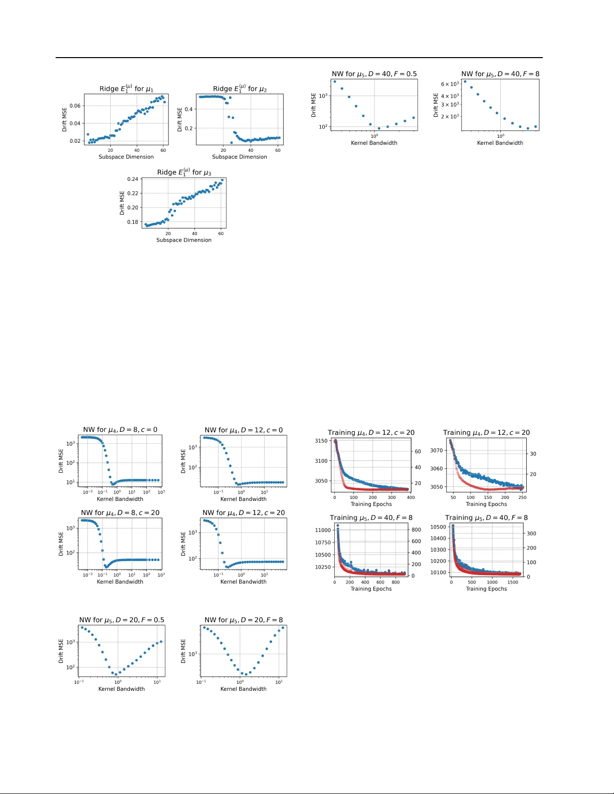
Drift Estimation for Stochastic Dif ferential Equations with Denoising Dif fusion Models Marcos T apia Costa 1 , 2 Nikolas Kantas 1 George Deligiannidis 2 February 23, 2026 Abstract W e study the estimation of time-homogeneous drift functions in multiv ariate stochastic dif feren- tial equations with known dif fusion coef ficient, from multiple trajectories observed at high fre- quency over a fixed time horizon. W e formu- late drift estimation as a denoising problem con- ditional on previous observ ations, and propose an estimator of the drift function which is a by- product of training a conditional diffusion model capable of simulating new trajectories dynam- ically . Across different drift classes, the pro- posed estimator was found to match classical methods in low dimensions and remained con- sistently competitive in higher dimensions, with gains that cannot be attributed to architectural de- sign choices alone. 1. Problem Statement Suppose one is interested in modelling a time series as a continuous-time stochastic differential equation (SDE), d Y t = µ ( Y t ) dt + σ dB t , t ∈ [0 , T ] , (1) where ( B t ) t ∈ [0 ,T ] is a D -dimensional Brownian motion and µ : R D → R D is a time-homogeneous drift func- tion. W e assume σ is known or well-estimated, i.e., us- ing the quadratic variation of a single path, see (Jacod, 1994; Barndorff-Nielsen & Shephard, 2002; Jacod & Prot- ter, 2012). W e also assume µ is locally Lipschitz to ensure a strong solution to (1) up to terminal time T , see (Karatzas & Shrev e, 2000). W e will inv estigate the case we are giv en a dataset D con- sisting of I ≫ 1 i.i.d. trajectories, each with J observa- tions of dimension D observed at times t j = j ∆ ∀ j ∈ { 1 , · · · , J } , such that D = { Y ( i ) t 1 , · · · , Y t J } i ∈ [ I ] , [ I ] := { 1 , · · · , I } and ∆ := t j +1 − t j is small. In our setting, the number of trajectories I and the number of discrete ob- servations J are fixed with a constant sampling frequency 1 Department of Mathematics, Imperial College London, UK 2 Department of Statistics, Univ ersity of Oxford, UK ∆ . W ithout loss of generality , we assume T = 1 and Y ( i ) 0 ∼ Q 0 , where Q 0 admits a density with respect to the Lebesgue measure dy 0 ; Q 0 ( dy 0 ) = q 0 ( y 0 ) dy 0 . W e will study the problem of estimating the drift function µ from the dataset D . 1.1. Drift estimation as a regr ession Letting Z t j := Y t j − Y t j − 1 , the solution o ver s ∈ [ t j − 1 , t j ] to (1) takes the form, Z t j = Z t j t j − 1 µ ( Y s ) ds + √ ∆ ω , ω ∼ N (0 , I ) . (2) For small ∆ , an Euler-Maruyama (EM) approximation to (2) abov e yields, b Z t j = µ ( Y t j − 1 )∆ + √ ∆ ω , ω ∼ N (0 , I ) (3) and the drift enters µ through the conditional mean: E h b Z t j | Y t j − 1 i = µ ( Y t j − 1 )∆ . (4) In our multiple trajectory setting, with I ≫ 1 , one could use (4) to learn µ by regressing states against increments through a nonparametric function D θ (Zhao et al., 2025), D θ ∗ = arg min θ 1 2 X i,j     D θ ( Y ( i ) t j − 1 ) − Z ( i ) t j    2 2  . (5) It is well known that in our fixed T , J, ∆ setting, the drift µ cannot be estimated consistently from a single trajectory (Jakobsen & Sørensen, 2015). Howe ver , in the multiple trajectory setting, (Zhao et al., 2025) provide asymptotic con ver gence guarantees for separable drift functions under conditions on the class of functions D θ . Y et, the drift esti- mator D θ ∗ can suf fer from high variance, as the drift con- tribution scales as O (∆) , and the diffusion noise scales as O ( √ ∆) (Gobet, 2002; Kutoyants, 2004), and the Fisher information per observation vanishes as ∆ → 0 . In high dimensions, this difficulty is further compounded by dete- riorating nonparametric regression con vergence rates with dimension, requiring significantly more data to achie ve the same accuracy as in lo wer dimensions (Tsybakov, 2009). 1 Drift Estimation for SDEs using Denoising Diffusion Models A general approach to mitigate variance in regression prob- lems is to inject additive Gaussian noise into the inputs, which acts as a form of T ikhonov regularisation on D θ (Bishop, 1995). More generally , under the loss in (5), re- gression with noisy inputs corresponds to learning the con- ditional expectation of the target giv en the corrupted in- put, i.e., learning a denoiser . Moreo ver , (Starnes & W eb- ster, 2025) show learning the denoiser from Gaussian per- turbations can smooth low variance, high curvature direc- tions during optimisation and lead to a better conditioned stochastic gradient descent problem. (V incent, 2011) fur- ther showed that such denoising objectiv es are equiv alent to score matching under Gaussian perturbations. Modern denoising diffusion models extend this principle by intro- ducing a controlled, multi-scale noising process and learn- ing denoisers across noise levels, with great success in im- age and video applications (Sohl-Dickstein et al., 2015; Ho et al., 2020; Song et al., 2021b). In this paper , we extend the methodology of denoising dif- fusion models to introduce a controlled noising process and deriv e an estimator for the drift µ . W e will propose a no vel construction for the estimator , and present systematic em- pirical results showing that the denoising-based estimator improv es out-of-sample performance in high-dimensional settings with strong interactions or chaotic dynamics, while remaining competitive when standard regression already generalises well. Theoretical guarantees as in (Zhao et al., 2025) are left for future work. 2. Related Literature 2.1. Drift estimation for stochastic differ ential equations The problem of estimating the drift function of an SDE has been extensi vely studied. In the single trajectory set- ting, (Kessler, 1997) derived an efficient estimator for the drift function of an ergodic scalar dif fusion observed at dis- crete times when transition densities are unknown. (Shoji & Ozaki, 1995) developed a pseudo-likelihood estimator from a locally linear approximation of the SDE, while (A ¨ ıt- Sahalia, 2002) used polynomial Hermite expansions of the transition density to obtain an approximate maximum like- lihood estimator . Nonparametric approaches were introduced through the kernel regression estimator of (W atson, 1964), and (Nadaraya, 1964) was first applied to Brownian SDEs by (Florens-Zmirou, 1993), who estimate both drift and dif fu- sion coefficients in scalar diffusions, and (Bandi & Phillips, 2003; 2007) provided uniform con ver gence rates for its ap- plication to high frequency financial data. Furthermore, (Dalalyan, 2006) deri ved a nonparametric estimator for ho- mogeneous drift functions that achie ves minimax optimal rates, while (Comte & Genon-Catalot, 2009; 2010) pro- posed penalised least squares projection methods to jointly estimate the drift and dif fusion coef ficients nonparametri- cally . More recently , (Oga & Koik e, 2023) dev elop theo- retical guarantees for multidimensional drift estimation for a class of deep neural networks, giv en a single path with many observ ations. In the multiple trajectory setting, which is the observ ation regime of this paper , (Bonalli & Rudi, 2025) used a Repro- ducing Kernel Hilbert Space approximation of the Fokker- Plank equation to estimate multidimensional non-linear drift functions. (Mohammadi et al., 2024) use Functional Data Analysis to develop a drift estimator gi ven sparse ob- servations. (Marie & Rosier, 2023) extend kernel smooth- ing estimators of the drift function to the multiple i.i.d. tra- jectory setting, while (Comte & Genon-Catalot, 2020; De- nis et al., 2021) extend penalised least squares estimators to the same setting. More recently , (Zhao et al., 2025) pro vide asymptotic con ver gence guarantees for separable drift esti- mation in a compact domain using feed-forward neural net- works. Their empirical e valuation, howe ver , is restricted to a single test drift function and assesses recov ery only along one coordinate of a high-dimensional system, leaving per- formance on fully coupled dynamics unexamined. 2.2. Score-based generati ve models Score-based generativ e models, or Denoising Diffusion Models (DDMs) , were introduced in (Ho et al., 2020) and (Song et al., 2021b), drawing ideas from score-matching (Hyvarinen & Dayan, 2005; V incent, 2011) and building on earlier work (Sohl-Dickstein et al., 2015). By using neu- ral networks to estimate the log density of a smoothed data distribution, i.e. the scor e , they hav e achieved state-of-the- art results in image generation (Ho et al., 2020; Dhariwal & Nichol, 2021; Saharia et al., 2022; Brooks et al., 2023), and hav e found numerous applications in video generation (Ho et al., 2022), molecule and drug design, (Xu et al., 2023; Corso et al., 2023), strategy testing (K oshiyama et al., 2021), and data sharing (Assefa, 2020). Their state-of-the-art performance across several domains, and the fact that they are less susceptible to training in- stabilities or mode-collapse, hav e established DDMs as the gold-standard in generative modelling (Dhariw al & Nichol, 2021). In particular , (Song & Ermon, 2019) ex- tended (Sohl-Dickstein et al., 2015) to a practical setting by formalising Stochastic Gradient Lange vin Dynamics (SGLD) as the latent variable process, while (Ho et al., 2020) introduced Denoising Diffusion Probabilistic Mod- els (DDPM). These approaches were unified under an SDE- based framew ork in (Song et al., 2021c), who show that the forward processes in DDPM and SGLD are discretisa- tions of continuous-time It ˆ o-SDEs. Further generalisations 2 Drift Estimation for SDEs using Denoising Diffusion Models hav e been achiev ed in recent years, see (Song et al., 2021a; Franzese et al., 2023; Zhang et al., 2023; Benton et al., 2024). Other contrib utions hav e proposed improvements to accelerate sampling or to improve sample quality , such as (Jolicoeur-Martineau et al., 2021; Bao et al., 2022; W atson et al., 2022; Xu et al., 2022; Rombach et al., 2022). Fi- nally , using ideas from optimal transport, (De Bortoli et al., 2021; Shi et al., 2022; 2023) dev eloped a parallel line of work, connecting diffusion models to Schr ¨ odinger bridge problems. 2 . 2 . 1 . L E A R N I N G T H E S C O R E F O R T I M E S E R I E S D A TA Beyond image and spatial data, score-based dif fusion mod- els have also been extensi vely applied to time-series set- tings, see (Lin et al., 2023) for a comprehensiv e surve y . While the methods re viewed belo w are not used directly in this work, they illustrate how diffusion models have been adapted to temporal and conditional structures, and there- fore provide rele vant conte xt for our setting. In the field of time series forecasting, (Lim et al., 2023) draw inspiration from the T imeGrad model in (Rasul et al., 2021; Kong et al., 2021) and the ScoreGrad model in (Y an et al., 2021) to propose the TSGM model, a conditional diffusion model that operates on a low-dimensional rep- resentation of the data. (Shen & Kwok, 2023) remov e the sequence-based architecture (LSTM, T ransformer) to achiev e non-autoregressi ve forecasting. For time-series with missing values, (T askhiro et al., 2021; Alcaraz & Strodthoff, 2023; K ollovieh et al., 2023) proposed condi- tional diffusion framew orks that impute unobserved en- tries. For long-horizon multiv ariate sequence generation, (Barancikov a et al., 2025) introduce SigDiffusion, which lev erages path signatures. In the domain of filtering, (Bao et al., 2022; 2024) applied score-based conditional diffu- sion models to non-linear filtering problems. 3. Background 3.1. Score-based diffusion models Score-based diffusion models are generativ e models that learn a rev ersible transformation between two distributions, p 0 and p 1 . (Song et al., 2021b) used a forward SDE to transform samples distributed according to p 0 to samples distributed according to p 1 . Defining γ ( τ ) = γ 0 + τ ( γ 1 − γ 0 ) , the forward SDE takes samples X 0 ∼ p 0 and diffuses them tow ards X 1 ∼ p 1 via a V ariance-Preserving SDE (VPSDE), dX τ = − 1 2 γ ( τ ) X τ dτ + p γ ( τ ) dW τ , τ ∈ [0 , 1] , (6) where ( W τ ) τ ∈ [0 , 1] is a D -dimensional Brownian motion, see Section 3.4 in (Song et al., 2021b). W e emphasise (6) is a different SDE to the data-generating process assumed in (1), and which defines the distribution p 0 . From (Anderson, 1982), the forward SDE in (6) admits a time-rev ersal which diffuses e X 0 ∼ p 1 back to e X 1 ∼ p 0 via, d e X τ =  1 2 e X τ + ∇ e X τ ln p τ ( e X τ )  γ ( τ ) dτ + p γ ( τ ) d f W τ , (7) such that e X τ d = X 1 − τ , f W τ d = W 1 − τ ∀ τ ∈ [0 , 1] , where d = means equal in distribution. The reverse-time SDE in (7) requires access to the score ∇ X τ ln p τ ( X τ ) which is not av ailable in closed form in general. (V incent, 2011; Song et al., 2021b) show that the oracle score-matching objectiv e is, l ( θ ) = Z 1 0 E h λ ( τ ) ∥ s θ ( τ , X τ ) − ∇ X τ ln p τ ( X τ ) ∥ 2 2 i dτ , where X 0 ∼ p 0 ( x 0 ) , X τ ∼ q τ ( x τ | X 0 ) and s θ : [0 , 1] × R D → R D is a neural network parameterised by θ . The function λ : [0 , 1] → R + is a positiv e weighting function, and q τ ( x τ | X 0 ) is the transition density of (6), q τ ( x τ | X 0 ) = N ( x τ ; β τ X 0 , σ 2 τ I ) , (8) where we have defined σ 2 τ = 1 − β 2 τ and β τ = exp  − 0 . 25 τ 2 ( γ 1 − γ 0 ) − 0 . 5 τ γ 0  . Howe ver , the objecti ve l ( θ ) cannot be e valuated in practice since we do not hav e access to the score. Under sufficient expressi vity of the neural network s θ , (V incent, 2011) show that the denoising score-matching objectiv e has the same global minimum as l ( θ ) , e l ( θ ) = Z 1 0 E h λ ( τ )   s θ ( τ , X τ ) − ∇ X τ ln q τ ( X τ | X 0 )   2 2 i dτ . (Song & Ermon, 2019), (Song et al., 2021b) proposed the weighting function λ ( τ ) = σ 2 τ to reduce the variance of the target ∇ X τ ln q τ ( X τ | X 0 ) = − σ − 2 τ ( X τ − β τ X 0 ) . In practice, the objecti ve e l ( θ ) is approximated via Monte Carlo sampling. In particular, one samples ( τ , X 0 ) ∼ U [ ϵ, 1] × p 0 and then X τ ∼ q τ ( x τ | X 0 ) for each sam- ple. The constant ϵ > 0 is chosen to av oid the explosion of the target since lim τ → 0 σ τ = 0 . 3.2. Conditional diffusion models Letting ( X 0 , Y ) ∼ p 0 ( x 0 , y ) , Y ∈ R D , (Song et al., 2021b), (T askhiro et al., 2021) apply score-based diffusion models to generate samples from p 0 ( x 0 | Y ) . For each fixed Y , applying the forw ard dif fusion (6) to X 0 induces a push-forward distribution p τ ( x τ | Y ) ∀ τ ∈ [0 , 1] . Similar to (7), the rev erse-time SDE for conditional generation is: d e X τ = h 1 2 e X τ + ∇ e X τ ln p τ ( e X τ | Y ) i γ ( τ ) dτ + p γ ( τ ) d f W τ . (9) 3 Drift Estimation for SDEs using Denoising Diffusion Models (Theorem 1, Appendices B.1-B.2) (Batzolis et al., 2021) show one can learn the conditional score in (9) consistently by minimising the following objecti ve, ˜ L ( θ ) = E h λ ( τ )   s θ ( τ , X τ , Y ) − ∇ X τ ln q τ ( X τ | X 0 )   2 2 i , (10) The conditional score can be written in terms of the de- noiser , ∇ X τ ln p τ ( X τ | Y ) = − X τ σ 2 τ + β τ σ 2 τ E [ X 0 | X τ , Y ] , (11) where the denoiser is giv en by , E [ X 0 | X τ , Y ] = Z R D x 0 p ( x 0 | X τ , Y ) dx 0 . (12) T o learn the denoiser directly , one can re-parameterise s θ using a network D θ , s θ ( τ , X τ , Y ) = − X τ σ 2 τ + β τ σ 2 τ D θ ( τ , X τ , Y ) (13) which can be plugged into the learning objective (10) for s θ to yield a learning objectiv e for D θ , ˜ L ( θ ) = E h ∥ D θ ( τ , X τ , Y ) − X 0 ∥ 2 2 i . (14) 4. Estimation of the drift function In this section, we study how to recover the drift µ ( Y ) from a denoising model trained to approximate the denoiser E [ X 0 | X τ , Y ] . W e exploit the Gaussian structure of the forward process to construct a Monte Carlo estimator for µ . 4.1. Data specification for conditional diffusion models Giv en trajectories Y ( i ) observed at times t j = j ∆ , recall we define ∀ j ∈ { 0 , . . . , J − 1 } the increment, Z ( i ) t j := Y ( i ) t j +1 − Y ( i ) t j . From (2), Z ( i ) t j depends on the past trajectory ( Y ( i ) t s ) j s =0 only through the current observation Y ( i ) t j . Consequently , under the time-homogeneous dynamics in (1), the condi- tional law of Z t j giv en Y t j is independent of j , and we work with generic pairs ( Y , Z ) , suppressing the indices i and j . Henceforth, X 0 will denote an increment from the data generating distribution p 0 ( x 0 | Y ) , and X τ is the diffused version of X 0 after applying the forward process q τ in (8). W e aim to learn an approximation D θ ( τ , X τ , Y ) to the de- noising target E [ X 0 | X τ , Y ] by minimising (10). 4.2. Learning the drift by denoising W e suppose henceforth that θ ∗ is the minimiser of (14) such that D θ ∗ ( τ , X τ , Y ) is the trained approximation to E [ X 0 | X τ , Y ] . W e also use the Euler-Maruyama approx- imation to the increment distribution in (4), p 0 ( x 0 | Y ) ≈ b p 0 ( x 0 | Y ) = N ( x 0 ; µ ( Y )∆ , ∆) to deriv e an estimator for µ . Under the VPSDE, the transition kernel q τ ( x τ | X 0 ) in (8) is a Gaussian linear in X 0 . Since the conditional distribu- tion b p 0 ( x 0 | Y ) is also Gaussian, a closed-form solution for the denoiser is obtained under the EM approximation, E [ X 0 | X τ , Y ] ≈ σ 2 τ ∆ σ 2 τ + β 2 τ ∆  µ ( Y ) + β τ σ 2 τ X τ  , and the drift is obtained through, µ ( Y ) = a ( τ ) X τ + b ∆ ( τ ) E [ X 0 | X τ , Y ] , (15) where, a ( τ ) := − β τ σ 2 τ , b ∆ ( τ ) := σ 2 τ + β 2 τ ∆ σ 2 τ ∆ . (16) For a giv en Y = y , let x ( k ) τ ∼ p τ ( x τ | y ) ∀ k ∈ [ K ] . W e can construct a single-sample estimator , b µ ( τ , x ( k ) τ , y ) = a ( τ ) x ( k ) τ + b ∆ ( τ ) D θ ∗ ( τ , x ( k ) τ , y ) , (17) where x ( k ) τ enters as a linear correction to the learned de- noiser , constructed in a way that preserves unbiasedness in the ideal case of (15). By averaging ov er the K samples x ( k ) τ , we can estimate the drift with, ¯ µ ( τ , y ) = 1 K X k ∈ [ K ] b µ ( τ , x ( k ) τ , y ) . (18) For sufficiently large K , the estimator ¯ µ ( τ , y ) removes the linear dependence of the rescaled denoiser on X τ in (15), and can be cast as a lo wer-v ariance alternative to ˆ µ ( τ , x ( k ) τ , y ) . W e emphasise that the Euler-Maruyama approximation used to deri ve (18) is not imposed during training, but only at the stage of drift estimation. 4.3. Choice of diffusion time for drift estimator T o implement the estimator in (18), a v alue of τ ∈ [0 , 1] must be chosen, and K samples x ( k ) τ ∼ p τ ( x τ | Y = y ) must be drawn. One expects there to exist an intermediate noise level 0 < τ < 1 for which the denoising problem is well conditioned and the drift approximation error in ¯ µ is low . W e propose setting τ = 1 as a con venient and empirically robust choice, as motiv ated in the remainder of this sec- tion. At τ = 1 , one should first sample K standard normal 4 Drift Estimation for SDEs using Denoising Diffusion Models random v ariables x ( k ) 1 ∼ N (0 , I ) . The drift in (17) is then, b µ (1 , x ( k ) 1 , y ) = a (1) x ( k ) 1 + b ∆ (1) D θ ∗ (1 , x ( k ) 1 , y ) , A veraging over all K samples yields ¯ µ ( y ) := ¯ µ (1 , y ) , ¯ µ ( y ) = 1 K X k ∈ [ K ] b µ (1 , x ( k ) 1 , y ) . (19) T o justify why τ = 1 is appropriate, we empirically in vesti- gate the dependence of the estimator ¯ µ ( τ , y ) on τ . In prin- ciple, samples x ( k ) τ ∼ p τ ( x τ | y ) can be drawn by sampling ( x 0 , y ) ∼ p 0 ( x 0 , y ) from the dataset D and applying the forward process q τ in (8). Howe ver , this approach is lim- ited to values of y observed in the dataset and scales poorly with dimension. Therefore, sampling x ( k ) τ from p τ ( x τ | y ) for different values of τ is implemented by simulating the rev erse diffusion (9), see (Song et al., 2021b; Karras et al., 2022), for details on different numerical implementations. The VPSDE forward process in (8) ensures X τ ≃ N (0 , I ) for large τ . W e can therefore sample x ( k ) 1 ∼ N (0 , I ) and run the reverse dif fusion in (9) to obtain approximate sam- ples from p τ ( x τ | y ) for intermediate dif fusion times. During validation, we set K = 10 and allow oracle access to the true drift to select the model which minimises the τ -av eraged drift mean-squared error (MSE), b θ = arg min θ E τ E h ∥ ¯ µ ( τ , Y ) − µ ( Y ) ∥ 2 2 i , W e choose to test this approach using two representati ve drift functions, µ (1) ( y ) = − y + sin(25 y ) , y ∈ R (20) µ (2) d ( y ) = − 4 a d y 3 d − 2 b d y d , y ∈ R D , d ∈ [ D ] (21) where a d > 0 , b d < 0 ∀ d ∈ [ D ] . Giv en a set of N points uniformly spaced y n ∈ R ⊂ R D , we approximate the drift MSE as, e 2 ( τ ) ≈ 1 N X n ∈ [ N ] ∥ µ ( y n ) − µ ( τ , y n ) ∥ 2 2 . (22) Figure 1 shows the error e 2 ( τ ) when estimating µ (1) for K ∈ { 1 , 10 , 100 } . In all cases, the drift MSE di verges as τ → 0 , as the approximation error in the network D θ ∗ is expected to increase for smaller τ (Song et al., 2021b). The error is minimised for τ ≈ 0 . 2 , but as K increases, the error curve becomes flat and less sensitiv e to τ , and larger values yield similar performance. Indeed, the bottom two panels in Figure 1 demonstrate accurate recov ery of µ (1) for τ ∈ { 0 . 2 , 1 } when K = 100 . Similarly , Figure 2 illustrates the drift error e 2 ( τ ) when estimating µ (2) for D = 8 (top row) and D = 12 (bot- tom row), exhibiting behaviour similar to Figure 1 ev en in higher dimensions. F igur e 1. The top-left panel shows the drift error e 2 ( τ ) when estimating µ (1) ; the top-right panel restricts the range of τ to τ ∈ [0 . 15 , 1] . The bottom row compares the true drift with ¯ µ ( τ , y ) for τ = 1 (left) and optimal τ ≈ 0 . 2 (right) for K = 100 . Positions Y are uniformly spaced between [ − 1 . 5 , 1 . 5] , co vering 99% of the training distribution. F igur e 2. The left panels show the drift error e 2 ( τ ) ∀ τ ∈ [0 , 1] ; the right panels restrict the range of τ to τ ∈ [0 . 15 , 1] . The top row sho ws the drift error e 2 ( τ ) µ (2) with D = 8 ; the bottom row shows the same for D = 12 . W e emphasise here that there is no closed form solution to selecting the optimal τ since the approximation error in D θ ∗ is architecture and data dependent. Further, the choice of forward noise schedule will impact the depen- dence of the estimator on τ , see Appendix A for a com- parison with the V ariance Exploding SDE. Therefore, there is no guarantee that a specific τ is optimal across archi- tectures and noise schedules. Moreover , the computational cost of simulating the re verse diffusion process is high. In contrast, sampling from the approximate terminal distribu- tion X 1 ∼ N (0 , I ) is cheap, and for large K , the error at τ = 1 is similar to the optimal error . As such, we suggest using τ = 1 to implement our estimator (19), and the re- sults in Section 5.4 confirm that ev en with this choice of τ , we achiev e competitiv e performance. 5 Drift Estimation for SDEs using Denoising Diffusion Models 5. Experiments 5.1. Evaluation Criterion W e ev aluate the performance of a drift estimator e µ using the time-integrated mean-squared error , E ( µ ) t = 1 t Z t 0 E ∥ e µ ( Y s ) − µ ( Y s ) ∥ 2 2 ds (23) where the expectation is o ver the law of the process ( Y s ) s . In practice, we approximate (23) in the following way . Let { Y ( i ) } i , i ∈ [ I ] be a set of i.i.d trajectories from (1) with J discrete observations. W e approximate (23) using ∀ j ∈ [ J ] , E ( µ ) j ∆ := 1 j I X i ∈ [ I ] X k ∈ [ j ]    e µ ( Y ( i ) t k ) − µ ( Y ( i ) t k )    2 2 , where I , J denote the number of trajectories and observa- tions, respectiv ely , used for error ev aluation. In contrast, I , J denote the number of training trajectories and obser- vations, respecti vely . 5.2. Implementation In all experiments, training datasets consist of I = 10 3 sample paths generated from an Euler discretisation of (1) with σ = 1 for t ∈ [0 , 1] at a frequency of ∆ = 256 − 1 . All drift estimators are fitted with fixed random seeds for reproducibility . In-sample errors are computed by simulat- ing I = 10 3 new trajectories ov er the in-sample horizon t ∈ [0 , 1] with ∆ = 256 − 1 , while out-of-sample errors are computed over t ∈ [0 , 20] . W e will denote by DN the de- noising estimator ¯ µ in (19) which uses the trained network D θ ∗ , see Appendix B for architectural details. For one dimensional drift functions, we compare DN against three nonparametric estimators used in drift es- timation under i.i.d trajectories. Specifically , we imple- ment the IID Nadaraya–W atson estimator (Marie & Rosier, 2023), a kernel-based estimator obtained by av eraging in- crements across independent trajectories; the IID Ridge (Denis et al., 2021), a spline-based least-squares estima- tor using B-spline bases with ridge regularization, and the IID Hermite projection (Comte & Genon-Catalot, 2020), which estimates the drift via least-squares projection onto a finite-dimensional Hermite basis, see Appendix C for more details. In higher dimensions, the computational and data require- ments of the Ridge and Hermite estimators of (Denis et al., 2021) and (Comte & Genon-Catalot, 2020) gro w exponen- tially with D (Zhao et al., 2025), and kernel-based estima- tors such as the Nadaraya W atson deteriorate rapidly , as seen in Appendix E. W e therefore omit them from the main text when estimating high dimensional drift functions. T o benchmark DN in high dimensions, we implement the proposed estimator in (Zhao et al., 2025), and refer to it as FC . The estimator FC is the output of a feed-forward ReLU network trained to regress the scaled increments ∆ − 1 X 0 from the states Y using (5), corresponding to a standard regression objectiv e, without any denoising mech- anism. W e follow (Zhao et al., 2025) in imposing sparsity and weight-clamping constraints on the network parame- ters during training. These constraints restrict the hypoth- esis class to separable drifts and are part of the estimator definition in (Zhao et al., 2025). For consistency , all neural- network based estimators are trained to tar get ∆ − 1 X 0 . Our denoising network D θ ∗ includes a learnable embed- ding applied to states Y , referred to as MLPStateMapper , which combines polynomial and Fourier features and feeds into the remaining network. It also includes a parallel one- dimensional con volutional module to capture local spatial structure in ( Y , X τ ) , see Appendix B for more details. As the performance of DN depends on both denoising-based training and architectural inducti ve biases in D θ ∗ , we intro- duce three control baselines to attempt to disentangle their contributions. W e denote by FC + the FC estimator with its parameter count matched to D θ ∗ , and remov e the sparsity and weight- clamping restrictions in (Zhao et al., 2025). W e further in- troduce FC + -Con v , which augments the fully connected layers with a similar parallel con volutional module as D θ ∗ . Both FC + , F C + -Con v are trained on the same objective as FC , i.e., the standard regression objectiv e. Therefore, estimators FC + , F C + -Con v help to isolate the ef fect of denoising by controlling for differences in model capacity and inductive bias. Finally , we define DN -Lin as a variant of DN in which the MLPStateMapper in D θ ∗ is replaced by a fully connected mapping, helping to isolate the effect of learned state embeddings in drift estimation. All estimators are selected by minimising the oracle error E ( µ ) j ∆ at the in-sample terminal time j ∆ = 1 . For the one- dimensional benchmarks, hyperparameters are chosen via grid search, see Appendix D. For neural network based esti- mators, ( FC , FC + , F C + -Con v , DN -Lin and DN ), we ev al- uate the error E ( µ ) 1 on I = 50 held-out trajectories at ev ery epoch and terminate training when E ( µ ) 1 has not improved ov er 100 epochs, see Appendix D for more details. Sensi- tivity to reduced training dataset size and to sampling fre- quency ∆ are explored in Appendix F and H, respectiv ely , and Appendix I provides a performance comparison when we use a feasible model selection objectiv e for DN , DN - Lin. 6 Drift Estimation for SDEs using Denoising Diffusion Models 5.3. T est Drift Functions For D = 1 , we consider the following one-dimensional drift functions, µ 1 ( y ) = − sin(2 y ) log(1 + 5 | y | ) , µ 2 ( y ) = − y + sin(25 y ) , µ 3 ( y ) = − y 3 + y . T o consider high-dimensional drifts derived from scalar po- tentials, we use the following parametric f amily , µ 4 ,d ( y ) = − 4 a d y 3 d − 2 b d y d − c 2 ψ ′ d ( y d )  ψ d − 1 ( y d − 1 ) + ψ d +1 ( y d +1 )  , where the coefficients satisfy a d > 0 , b d < 0 , and c is a coupling constant. F or c = 0 , µ 4 collapses to a separa- ble bi-stable potential with wells at y ∗ ,d = ± q − b d 2 a d . For c > 0 , coordinate interaction is introduced via ψ d ( y d ) = exp  − ( y 2 d − y 2 ∗ ,d ) 2 2 s 2 d  , and s d = √ cy ∗ ,d . T o consider non-potential and chaotic dynamics, we use the following drift, ∀ d ∈ { 0 , ..., D − 1 } and F > 0 , µ 5 ,d ( y ) = ( y d +1 − y d − 2 ) y d − 1 − y d + F , where indices are taken modulo D . For F < 1 , µ 5 defines the Lorenz-96 system which exhibits stable be- haviour , whereas chaotic behaviour emerges for standard choices such as F = 8 (Lorenz, 1996). 5.4. Results 5 . 4 . 1 . I N S A M P L E R E S U LT S T able 1 reports final-time in-sample errors E ( µ ) 1 for the one- dimensional benchmarks. The denoising-based estimator attains errors of the same order of magnitude as classical nonparametric methods, and Figure 3 illustrates that it ac- curately recov ers the structure of the drift. T able 1. In-sample drift errors E ( µ ) 1 , for µ 1 , µ 2 , µ 3 . Best estimator is starred, second-best is underlined. E ( µ ) 1 DN NW Hermite Ridge µ 1 0.02127 0.04564 0 . 007621 ∗ 0.02382 µ 2 0 . 01870 ∗ 0.1320 0.5049 0.0574 µ 3 0.00754 0.01464 0 . 005082 ∗ 0.1739 F igur e 3. Panels (left to right) correspond to µ 1 , µ 2 , µ 3 . T rue drift against DN drift. Shaded region shows 10 − 90% quantile env e- lope ov er K . State values cov er 99% of the training distrib ution. In higher dimensions, T able 2 shows that the denoising es- timator DN achie ves the lowest in-sample error when esti- mating the bistable drift µ 4 across both separable ( c = 0 ) and strongly coupled ( c = 20 ) regimes. In the separable case, ( DN -Lin) performs poorly in relation to DN , sug- gesting that denoising-based drift estimation depends on an inductiv e bias aligned with the drift structure in order to accurately learn the drift o ver the in-sample distrib ution. T able 2. In-sample drift errors E ( µ ) 1 , for µ 4 . Best estimator is starred, second-best is underlined. c D DN DN -Lin FC + -Con v FC + F C 0 8 1.047 ∗ 6.941 3.898 8.865 7.687 12 1.681 ∗ 11.294 6.316 14.276 14.157 20 8 8.490 ∗ 10.335 9.048 16.287 35.365 12 10.660 ∗ 13.648 14.076 29.528 46.166 Figure 4 overlays the true and estimated drift DN for se- lected dimensions of µ 4 , illustrating accurate recovery in intermediate dimensions and expected degradation in the highest-index dimension. F igur e 4. T rue drift against the DN drift for µ 4 , c = 0 . State values cover 99% of the training distribution in each dimension. T op panels show dimensions 3 (left) and 8 (right) for D = 8 . Bottom panels show dimensions 3 (left) and 12 (right) for D = 12 . Shaded region denotes 10 − 90% quantile en velope o ver K . T able 3 reports in-sample results for the Lorenz 96 drift µ 5 . Performance is dominated by architectural inductiv e bias, as estimators with con volutional architectures ( DN , DN -Lin, FC + -Con v) achiev e similar accuracy while fully connected baselines perform poorly . T able 3. In-sample drift errors E ( µ ) 1 , for µ 5 . F D DN DN -Lin FC + -Con v FC + F C 1 2 20 4.870 3.127 ∗ 3.733 18.554 49.862 40 9.596 7.766 ∗ 11.940 44.764 62.988 8 20 9.542 5.725 ∗ 11.486 127.103 926.707 40 17.898 12.203 ∗ 16.306 1263.290 2583.505 7 Drift Estimation for SDEs using Denoising Diffusion Models Overall, the results indicate that denoising-based estima- tors yield the strongest in-sample performance when paired with a network whose inducti ve bias is aligned with the underlying dynamics. Howe ver , since all networks are se- lected by oracle in-sample error during training, these re- sults reflect best-case fitting and may not be indicativ e of the relati ve generalisation beha viour of denoising and stan- dard regression estimators. 5 . 4 . 2 . O U T O F S A M P L E R E S U LT S W e e v aluate out-of-sample (OOS) performance by simulat- ing trajectories be yond the training horizon, where the sys- tem in (1) ev olves into regions of state space not observed during training. T able 4 reports final-time OOS errors for the bistable drift µ 4 . In the non-separable regime ( c = 20 ), the denois- ing estimators ( DN , DN -Lin) achiev e the lowest OOS er - ror compared to all standard regression baselines across di- mensions. Figure 5 sho ws that the OOS error of DN gro ws more slowly over time, leading to increasing separation from FC + -Con v . This advantage persists e ven when the F C + -Con v baseline is augmented with the MLPStateMap- per state embedding (see Appendix G), suggesting that the performance gap of DN is not explained by architecture alone. T able 4. Final-time OOS drift errors E ( µ ) 20 , for µ 4 . c D DN DN -Lin F C + -Con v FC + F C 0 8 1.546 ∗ 11.800 9.744 14.129 14.365 12 2.314 ∗ 16.616 8.344 21.523 23.658 20 8 50.919 ∗ 67.297 76.061 70.134 67.299 12 81.721 ∗ 115.750 121.379 182.499 105.854 F igur e 5. OOS E ( µ ) j ∆ for µ 4 , c = 20 , for DN , and FC + -Con v . Shaded region shows 10 − 90% quantile env elope over test tra- jectories I . T able 5 reports OOS results for the Lorenz 96 drift µ 5 . In the stable regime ( F = 0 . 5 ), the estimators with conv o- lutional networks achieve comparable OOS performance. In the chaotic regime ( F = 8 ), the denoising-based esti- mator DN -Lin consistently attains lower OOS error than F C + -Con v across dimensions. Since both estimators share the same inductiv e bias, these results suggest a generalisa- tion benefit attributable to the denoising training objective rather than architectural differences. The denoising variant DN underperforms in this setting, reflecting misalignment of the MLPStateMapper state embedding with the Lorenz 96 dynamics. Figure 6 shows that while OOS errors sta- bilise over time, DN -Lin plateaus at a lower error level than standard regression. T able 5. Final-time OOS drift error E ( µ ) 20 , for µ 5 . F D DN DN -Lin F C + -Con v FC + F C 1 2 20 8.718 12.024 7.920 ∗ 44.376 56.041 40 12.198 11.134 ∗ 12.802 99.322 167.826 8 20 3973 172.786 ∗ 226.361 7457 8425 40 1243 332.905 ∗ 527.726 16280 17656 F igur e 6. OOS E ( µ ) j ∆ for µ 5 , F = 8 comparing the DN -Lin , FC + - Con v estimators. Shaded region shows 10 − 90% quantile en ve- lope across test trajectories I . T aken together , the OOS results for µ 4 and µ 5 suggest stan- dard regression, when paired with an architecture aligned the underlying drift, can achiev e strong in-sample perfor- mance, yet may generalise poorly out of sample in strongly coupled or chaotic dynamics. In these settings, the denois- ing estimator with an appropriate architecture provides im- prov ed generalisation, while remaining competitiv e when networks trained via standard regression already generalise well. 6. Conclusion This paper adapts score-based conditional dif fusion models to the problem of high-dimensional drift estimation from discretely observed trajectories. By introducing controlled Gaussian corruption to the observed increments, we train a neural network to learn the denoiser of each increment conditional on the previous state. Using the trained net- work, we derived an estimator for the drift through a first- order approximation of the data-generating process. Across a range of drift structures and dimensions, our results sho w that denoising can complement architectural inducti ve bias to improv e out-of-sample robustness in settings with strong interactions or chaotic dynamics. In contrast, when stan- dard regression already generalises stably out of sample, denoising can remain competiti ve. Several important ques- tions remain open. These include dev eloping a theoretical understanding for how different noise schedules affect the bias-variance properties of the estimator under specific ar- chitectures, as well as extending the estimator construction to incorporate higher order approximations of the denois- ing target. 8 Drift Estimation for SDEs using Denoising Diffusion Models 7. Impact Statement This paper presents work whose goal is to advance the field of Machine Learning. There are many potential societal consequences of our work, none which we feel must be specifically highlighted here. References A ¨ ıt-Sahalia, Y . Maximum likelihood estimation of dis- cretely sampled diffusions: A closed-form approxima- tion approach. Econometrica , 70(1):223–262, 2002. Alcaraz, J. M. L. and Strodthoff, N. Diffusion-based condi- tional ecg generation with structured state space models, 2023. Anderson, B. D. O. Rev erse-time diffusion equation mod- els. Stochastic Processes and their Applications , 12(3): 313–326, 1982. doi: 10.1016/0304- 4149(82)90051- 5. Assefa, S. Generating Synthetic Data in Finance: Opportunities, Challenges and Pitfalls . SSRN, 2020. URL http://dx.doi.org/10.2139/ ssrn.3634235 . Bandi, F . M. and Phillips, P . C. B. Fully nonparametric estimation of scalar dif fusion models. Econometrica , 71 (1):241–283, 2003. Bandi, F . M. and Phillips, P . C. B. A simple approach to the parametric estimation of diffusion processes. Journal of Econometrics , 141(1):62–94, 2007. Bao, F ., Li, C., Zhu, J., and Zhang, B. Analytic-DPM: an analytic estimate of the optimal rev erse variance in dif- fusion probabilistic models. In International Conference on Learning Repr esentations , 2022. URL https:// openreview.net/forum?id=0xiJLKH- ufZ . Bao, F ., Zhang, Z., and Zhang, G. A score-based filter for nonlinear data assimilation. Journal of Computational Physics , 514:113207, Oct 2024. ISSN 0021-9991. doi: 10.1016/j.jcp.2024.113207. Barancikov a, B., Huang, Z., and Salvi, C. Sigdif- fusions: Score-based diffusion models for time se- ries via log-signature embeddings. In International Confer ence on Learning Representations (ICLR) 2025 , 2025. URL https://openreview.net/forum? id=Y8KK9kjgIK . Barndorff-Nielsen, O. E. and Shephard, N. Econometric analysis of realized volatility and its use in estimating stochastic volatility models . J ournal of the Royal Statis- tical Society: Series B , 64(2):253–280, 2002. Batzolis, G., Stanczuk, J., Sch ¨ onlieb, C.-B., and Etmann, C. Conditional image generation with score-based dif- fusion models. In Advances in Neural Information Pr o- cessing Systems , v olume 34, 2021. Benton, J., Shi, Y ., De Bortoli, V ., Deligiannidis, G., and Doucet, A. From denoising dif fusions to denoising markov models. Journal of the Royal Statistical Society , Series B: Statistical Methodology , 86(2):286–301, Apr 2024. doi: 10.1093/jrsssb/qkae005. Bishop, C. M. T raining with noise is equiv alent to tikhonov regularization. Neural Computation , 7(1):108– 116, 1995. doi: 10.1162/neco.1995.7.1.108. Bonalli, R. and Rudi, A. Non-parametric Learning of Stochastic Differential Equations with Non-asymptotic Fast Rates of Con ver gence. F oundations of Computa- tional Mathematics , 25(3), mar 2025. doi: 10.1007/ s10208- 025- 09705- x. Brooks, T ., Holynski, A., and Efros, A. A. Instructpix2pix: Learning to follow image editing instructions. In Pro- ceedings of the IEEE/CVF Conference on Computer V i- sion and P attern Recognition (CVPR) , pp. 19530–19539, 2023. doi: 10.1109/CVPR52688.2023.01908. Comte, F . and Genon-Catalot, V . Nonparametric drift esti- mation for diffusion processes. Stochastic Processes and their Applications , 119(12):4088–4123, 2009. Comte, F . and Genon-Catalot, V . Adapti ve estimation of the drift function for ergodic dif fusions: A penalized projection approach. Bernoulli , 16(3):617–652, 2010. Comte, F . and Genon-Catalot, V . Nonparametric drift es- timation for i.i.d. paths of stochastic differential equa- tions. The Annals of Statistics , 48(6):3336–3365, 2020. doi: 10.1214/19- A OS1933. URL https://doi. org/10.1214/19- AOS1933 . Corso, G., St ¨ ark, H., Jing, B., Barzilay , R., and Jaakk ola, T . Diffdock: Diffusion steps, twists, and turns for molecu- lar docking. In Pr oceedings of the International Confer- ence on Learning Repr esentations (ICLR) , 2023. URL https://arxiv.org/abs/2210.01776 . Dalalyan, A. S. Sharp adapti ve estimation of the drift func- tion for ergodic diffusions. Annals of Statistics , 34(1): 291–376, 2006. De Bortoli, V ., Thornton, J., Heng, J., and Doucet, A. Dif- fusion Schr ¨ odinger Bridge with Applications to Score- Based Generative Modeling. In Advances in Neural In- formation Pr ocessing Systems , 2021. 9 Drift Estimation for SDEs using Denoising Diffusion Models Denis, C., Dion-Blanc, C., and Martinez, M. A ridge estimator of the drift from discrete repeated observa- tions of the solution of a stochastic differential equa- tion. Bernoulli , 27(4):2675–2713, 2021. doi: 10.3150/ 21- BEJ1327. URL https://doi.org/10.3150/ 21- BEJ1327 . Dhariwal, P . and Nichol, A. Q. Diffusion models beat GANs on image synthesis. In Beygelzimer , A., Dauphin, Y ., Liang, P ., and V aughan, J. W . (eds.), Advances in Neural Information Pr ocessing Systems , 2021. URL https://openreview.net/forum? id=AAWuCvzaVt . Florens-Zmirou, D. On estimating the dif fusion coef ficient from discrete observ ations. J ournal of Applied Pr oba- bility , 30(4):790–804, 1993. Franzese, G., Corallo, G., Rossi, S., Heinonen, M., Filip- pone, M., and Michiardi, P . Continuous-T ime Functional Diffusion Processes. In Advances in Neural Information Pr ocessing Systems , 2023. Gobet, E. Lan property for ergodic diffusions with discrete observations. Annales de l’Institute Henri P oincar ´ e, Pr obabilit ´ e et Statistiques , 38(4):651–676, 2002. doi: 10.1016/S0246- 0203(02)01107- X. Ho, J., Jain, A., and Abbeel, P . Denoising dif fusion probabilistic models. In Larochelle, H., Ranzato, M., Hadsell, R., Balcan, M., and Lin, H. (eds.), Ad- vances in Neural Information Pr ocessing Systems , volume 33, pp. 6840–6851. Curran Associates, Inc., 2020. URL https://proceedings.neurips. cc/paper_files/paper/2020/file/ 4c5bcfec8584af0d967f1ab10179ca4b- Paper. pdf . Ho, J., Saharia, C., Chan, W ., Fleet, D. J., Norouzi, M., and Salimans, T . V ideo diffusion models. In Advances in Neural Information Pr ocessing Systems (NeurIPS) , volume 35, pp. 8633–8646, 2022. URL https:// arxiv.org/abs/2204.03458 . Hyvarinen, A. and Dayan, P . Estimation of non-normalized statistical models by score matching. J ournal of Machine Learning Resear ch , 6(4), 2005. Jacod, J. Limit of random measures associated with the increments of a semimartingale. Stochastic Processes and their Applications , 50(1):41–60, 1994. Jacod, J. and Protter, P . Discr etization of Pr ocesses , vol- ume 67. Springer , 2012. Jakobsen, N. M. and Sørensen, M. Efficient estimation for diffusions sampled at high frequency over a fixed time interval. T echnical Report 2015-33, CREA TES, Aarhus Univ ersity , 2015. URL https://ideas.repec. org/p/aah/create/2015- 33.html . Jolicoeur-Martineau, A., Li, K., Pich ´ e-T aillefer, R., Kach- man, T ., and Mitliagkas, I. Gotta go fast when generating data with score-based models, 2021. Karatzas, I. and Shrev e, S. E. Br ownian Motion and Stochastic Calculus , volume 113. Springer , 2 edition, 2000. Karras, T ., Aittala, M., Aila, T ., and Laine, S. Elucidat- ing the design space of diffusion-based generativ e mod- els, 2022. URL 00364 . Kessler , M. Estimation of an ergodic diffusion from dis- crete observations. Scandinavian Journal of Statistics , 24(2):211–229, 1997. Kim, B. J., Kawahara, Y ., and Kim, S. W . The disappear- ance of timestep embedding in modern time-dependent neural networks. arXiv pr eprint arXiv:2405.14126 , 2024. URL 14126 . Kingma, D. P . and Ba, J. Adam: A method for stochastic optimization. In International Conference on Learning Repr esentations , 2015. K ollovieh, M., Ansari, A. F ., Bohlke-Schneider , M., Zschiegner , J., W ang, H., and W ang, Y . Predict, refine, synthesize: Self-guiding diffusion models for probabilis- tic time series forecasting. In Advances in Neural Infor- mation Pr ocessing Systems (NeurIPS) 36 , 2023. K ong, Z., Ping, W ., Huang, J., Zhao, K., and Catanzaro, B. Diffw av e: A versatile diffusion model for audio synthe- sis. In International Confer ence on Learning Repr esen- tations (ICLR) 2021 , 2021. K oshiyama, A., Firoozye, N., and T releav en, P . Gener- ativ e adversarial networks for financial trading strate- gies fine tuning and combination. Quantitative F inance , 21(5):797–813, 2021. doi: 10.1080/14697688.2020. 1790635. URL https://doi.org/10.1080/ 14697688.2020.1790635 . Kutoyants, Y . A. Statistical Infer ence for Er godic Dif- fusion Pr ocesses . Springer , 2004. doi: 10.1007/ 978- 1- 4471- 3866- 2. Lim, H., Kim, M., Park, S., and Park, N. Regular time- series generation using SGM. In Advances in Neural Information Pr ocessing Systems (NeurIPS) 36 , 2023. Lin, L., Li, Z., Li, R., Li, X., and Gao, J. Diffusion Models for T ime Series Applications: A Surve y, 2023. 10 Drift Estimation for SDEs using Denoising Diffusion Models Lorenz, E. N. Predictability: A problem partly solved. Pr o- ceedings of the Seminar on Pr edictability , 1:1–18, 1996. Marie, N. and Rosier, A. Nadaraya–watson estimator for i.i.d. paths of diffusion processes. Scandinavian J ournal of Statistics , 50(2):589–637, 2023. doi: 10.1111/sjos. 12593. URL https://onlinelibrary.wiley. com/doi/abs/10.1111/sjos.12593 . Mohammadi, N., Santoro, L., and Panaretos, V . M. Non- parametric Estimation for SDE with Sparsely Sampled Paths: an FD A Perspectiv e. Stochastic Pr ocesses and Their Applications , 2024. doi: 10.1016/j.spa.2023. 104239. Nadaraya, E. A. On estimating regression. Theory of Pr ob- ability & Its Applications , 9(1):141–142, 1964. Oga, A. and K oike, Y . Drift estimation for a multi- dimensional diffusion process using deep neural networks. Stochastic Pr ocesses and Their Appli- cations , 2023. doi: 10.1016/j.spa.2023.104240. URL https://www.sciencedirect.com/ science/article/pii/S0304414923002120 . Rasul, K., Seward, C., Schuster , I., and V ollgraf, R. Au- toregressi ve denoising dif fusion models for multiv ari- ate probabilistic time series forecasting. In Meila, M. and Zhang, T . (eds.), Pr oceedings of the 38th Interna- tional Confer ence on Machine Learning , volume 139, pp. 8857–8868. PMLR, 2021. Rombach, R., Blattmann, A., Lorenz, D., Esser , P ., and Ommer , B. High-resolution image synthesis with la- tent diffusion models. In Proceedings of the IEEE/CVF Confer ence on Computer V ision and P attern Recogni- tion (CVPR) , pp. 10684–10695, 2022. URL https: //arxiv.org/abs/2112.10752 . Saharia, C., Chan, W ., Saxena, S., Li, L., Whang, J., Den- ton, E., Seyed Ghasemipour , K., A yan, B. K., Mahdavi, S. S., Lopes, R. G., Salimans, T ., Ho, J., Fleet, D. J., and Norouzi, M. Photorealistic text-to-image diffusion models with deep language understanding. In Advances in Neural Information Pr ocessing Systems (NeurIPS) , volume 35, pp. 36479–36494, 2022. URL https: //arxiv.org/abs/2205.11487 . Shen, L. and Kwok, J. Non-autoregressi ve conditional dif- fusion models for time series prediction. In Pr oceedings of the 40th International Confer ence on Machine Learn- ing (ICML) , 2023. Shi, Y ., Bortoli, V . D., Deligiannidis, G., and Doucet, A. Conditional simulation using diffusion schr ¨ odinger bridges, 2022. Shi, Y ., De Bortoli, V ., Campbell, A., and Doucet, A. Dif fu- sion schr ¨ odinger bridge matching. In Advances in Neu- ral Information Pr ocessing Systems (NeurIPS) 36 , 2023. Shoji, I. and Ozaki, T . Estimation for nonlinear stochas- tic dif ferential equations by a local linearization method. Stochastic Analysis and Applications , 13(1):1–25, 1995. Sohl-Dickstein, J., W eiss, E., Maheswaranathan, N., and Ganguli, S. Deep unsupervised learning using nonequi- librium thermodynamics. In Bach, F . and Blei, D. (eds.), Pr oceedings of the 32nd International Confer- ence on Machine Learning , volume 37, pp. 2256–2265. PMLR, 2015. URL https://proceedings.mlr. press/v37/sohl- dickstein15.html . Song, J., Meng, C., and Ermon, S. Denoising dif fu- sion implicit models. In International Confer ence on Learning Representations , 2021a. URL https:// openreview.net/forum?id=St1giarCHLP . Song, Y . and Ermon, S. Generativ e modeling by estimating gradients of the data distrib ution. In W allach, H., Larochelle, H., Beygelzimer , A., d’Alche Buc, F ., Fox, E., and Garnett, R. (eds.), Advances in Neural Information Pr ocessing Sys- tems , volume 32. Curran Associates, Inc., 2019. URL https://proceedings.neurips. cc/paper_files/paper/2019/file/ 3001ef257407d5a371a96dcd947c7d93- Paper. pdf . Song, Y ., Sohl-Dickstein, J., Kingma, D. P ., K umar , A., Er - mon, S., and Poole, B. Score-based generati ve modeling through stochastic differential equations, 2021b. URL https://arxiv.org/abs/2011.13456 . Song, Y ., Sohl-Dickstein, J., Kingma, D. P ., Kumar , A., Ermon, S., and Poole, B. Score-based genera- tiv e modeling through stochastic differential equations. In International Conference on Learning Repr esenta- tions , 2021c. URL https://openreview.net/ forum?id=PxTIG12RRHS . Starnes, A. and W ebster , C. Improved performance of stochastic gradients with gaussian smoothing. In Op- timization, Learning Algorithms and Applications , vol- ume 2617 of Communications in Computer and Infor- mation Science . Springer , Cham, 2025. doi: 10.1007/ 978- 3- 032- 00137- 5 11. T askhiro, Y ., Song, J., Song, Y ., and Ermon, S. Csdi: Con- ditional score-based diffusion models for probabilistic time series imputation. In Beygelzimer , A., Dauphin, Y ., Liang, P ., and V aughan, J. W . (eds.), Advances in Neural Information Pr ocessing Systems , 2021. URL https: //openreview.net/forum?id=VzuIzbRDrum . 11 Drift Estimation for SDEs using Denoising Diffusion Models Tsybakov , A. B. Intr oduction to Nonparametric Estima- tion . Springer , 2009. doi: 10.1007/b13794. V incent, P . A connection between score matching and de- noising autoencoders. Neural computation , 23(7):1661– 1674, 2011. W atson, D., Ho, J., Norouzi, M., and Chan, W . Learning to efficiently sample from diffusion probabilistic models, 2022. URL https://openreview.net/forum? id=LOz0xDpw4Y . W atson, G. S. Smooth regression analysis. Sankhy ¯ a: The Indian Journal of Statistics, Series A , 26(4):359–372, 1964. Xu, M., Po wers, A. S., Dror , R. O., Ermon, S., and Leskov ec, J. Geometric latent diffusion mod- els for 3d molecule generation. In Pr oceedings of the 40th International Confer ence on Machine Learning (PMLR) , v olume 202, pp. 38592–38610. PMLR, 2023. URL https://proceedings.mlr. press/v202/xu23n.html . Xu, Y ., Ma, X., Zhang, J., Chen, Y ., W ang, Y ., Zhao, H., W ang, Y ., Zhang, C., Ji, R., and Xu, H. Fast sam- pling of dif fusion models with exponential integrator . arXiv preprint arXiv:2204.13902 , 2022. URL https: //arxiv.org/abs/2204.13902 . Y an, T ., Zhang, H., Zhou, T ., Zhan, Y ., and Xia, Y . Score- grad: Multiv ariate probabilistic time series forecasting with continuous energy-based generativ e models, 2021. URL . Zhang, L., Ma, H., Zhu, X., and Feng, J. Preconditioned Score-based Generative Models. In Advances in Neural Information Pr ocessing Systems , 2023. Zhao, Y ., Liu, Y ., and Hoffmann, M. Drift estimation for diffusion processes using neural networks based on discretely observed independent paths. arXiv preprint arXiv:2511.11161 , 2025. URL https://arxiv. org/abs/2511.11161 . A. Sensitivity to f orward noising process In this section, we motiv ate why the forward noising pro- cess q τ ( X τ | X 0 ) needs to be carefully chosen to ensure our denoising estimator (19) accurately recov ers the drift func- tion. Recall the transition kernel for the VPSDE noising process, q τ ( x τ | X 0 ) = N ( x τ ; β τ X 0 , σ 2 τ I ) , where β τ = exp( − 0 . 25 τ 2 ( γ 1 − γ 0 ) − 0 . 5 τ γ 0 ) and σ 2 τ = 1 − β 2 τ . (Song et al., 2021b) define an alternativ e noising process (the V ariance Exploding SDE), which takes sam- ples X 0 ∼ p 0 and dif fuses them with the forward transition density , q VE τ ( x τ | X 0 ) = N ( x τ ; X 0 , ϕ 2 τ I ) , (24) where ϕ τ = ϕ 0 ( ϕ 1 /ϕ 0 ) τ , ∀ τ ∈ [ ϵ, 1] . As in the VPSDE process, ϵ > 0 is chosen to a void vanishing variance as τ → 0 . Howe ver , in contrast to the VPSDE process, where noise v ariance σ 2 τ increases smoothly and saturates at 1 , the noise variance ϕ 2 τ in VESDE increases exponentially . Un- der uniform sampling in τ , this concentrates most training mass at low marginal noise levels. Consequently , the de- noising estimator is trained predominantly in high signal- to-noise regimes, where learning the denoising target is hardest. By comparison, the VPSDE distributes training more ev enly across signal-to-noise ratios. As such, given the same maximum noise le vels ϕ 1 = σ 1 , the VESDE pro- cess spends more time in lower -noise regimes, where de- noising is hardest. W e extend the experiments in Section 4.3 by dif fusing the observed increments X 0 with the VESDE noising kernel in (24). W e consider two VESDE variants. In VESDE- Matched, we set ϕ 1 = 1 to match the maximum marginal variance in the VPSDE. In VESDE-Larger , we increase the maximum marginal noise to ϕ 1 = 15 to compensate for the concentration of training mass at low noise le vels under VESDE-Matched. In both cases, ϕ 0 = 0 . 03 , and we set ϵ = 6 . 5 × 10 − 2 in VESDE-Matched and ϵ = 5 × 10 − 2 in VESDE-Lar ger in both training and e valuation to ensure the minimum marginal variance for both processes is iden- tical to that of the VPSDE process in Section 4.3. 12 Drift Estimation for SDEs using Denoising Diffusion Models F igur e 7. The top panels shows the drift error e 2 ( τ ) when esti- mating µ (1) ; the bottom panels compares the true drift to the esti- mated drift at τ = 1 . Positions Y are uniformly spaced between [ − 1 . 5 , 1 . 5] , covering 99% of the training distribution. F igur e 8. Drift error e 2 ( τ ) for µ (2) with D = 8 for VESDE- Matched (left) and VESDE-Larger (right). F igur e 9. Drift error e 2 ( τ ) for µ (2) with D = 12 for VESDE- Matched (left) and VESDE-Larger (right). As in the VPSDE case, Figures 7-9 show increasing K re- duces the drift MSE uniformly across τ for both VESDE variants. Howe ver , for fixed K , VESDE-Matched ex- hibits uniformly larger errors than VESDE-Larger . This gap is most pronounced for large diffusion times, where the forw ard process in VESDE-Larger has higher variance. T aken together , these results show that matching maximum marginal variance is insufficient for accurate drift estima- tion, and that effecti ve denoising requires adequate cov er- age of high noise regimes during training. B. Denoising Network Ar chitecture The architecture described in this section corresponds to the denoising network used for DN . The variant DN -Lin is obtained by removing the MLPStateMapper component (see Figure 11 and replacing it with a fully connected map- ping of matching output dimension, and no other module is changed. The network for DN is constructed such that the output is giv en by , D θ ( τ , X τ , Y ) = f θ ( Y ) + g θ ( X τ , Y ) + m θ ( g θ , τ ) . Figure 10 summarises the main components of the denoiser network architecture. The path followed by modules high- lighted in blue represents the implementation of g θ as a se- quence of 1 D con volutional neural networks and a single 1 D con volutional residual layer . The function m θ , high- lighted in orange, conditions the network on the diffusion time through a fully connected residual layer . The archi- tecture for m θ is motiv ated by the vanishing dependence of traditional diffusion models on the diffusion time (Kim et al., 2024). F igur e 10. Score network D θ used for DN . In prior dif fusion model architectures, the conditioning mapping f θ is often implemented using sequence-based architectures such as Long Short-T erm Memory (LSTM) networks or T ransformers (Y an et al., 2021; Corso et al., 2023; Lim et al., 2023; Saharia et al., 2022). These ar- chitectures maintain an internal state that evolv es with the history of observed inputs. In this paper , f θ is imple- mented using the MLPStateMapper , see Figure 11, which defines a non-linear feature mapping of the observed state Y without maintaining a recurrent or attention-based state. This design reflects the Markovian dependence structure induced by the data-generating SDE in (1). The mapping is constructed by combining multiple feature pathways: element-wise polynomial features ( Y , Y 2 , Y 3 ) , a learned global non-linear transformation implemented as a linear– ELU block, and Fourier features. The Fourier features are modulated by a learnable scalar gate, allo wing their contri- bution to be adaptively scaled during training. All feature components are concatenated and passed through a two- layer fully connected network to produce the final output in R D . The number of trainable parameters in D θ scales as T ( D ) = 2 D 2 + O ( D ) + O (1) . The quadratic dependence on the time-series dimensionality arises from the first 1 D con volution in g θ , see Figure 10, although the constant term in T ( D ) is much lar ger than the linear or quadratic terms. 13 Drift Estimation for SDEs using Denoising Diffusion Models F igur e 11. MLPStateMapper module. It provides an induc- tiv e bias towards polynomial and Fourier features, which can be learned from the data. C. Baselines C.1. IID Nadaraya-W atson Estimator In (Marie & Rosier, 2023), the authors improve the stan- dard Nadaraya-W atson estimator for the drift function by av eraging over I IID sample paths observed discretely J times. Assuming each path is defined on the same uniform time grid with ∆ = t j +1 − t j , the discrete-time estimator for the drift function is giv en by , b b J , I ,h ( y ) = c bf J , I ,h ( y ) b f J , I ,h ( y ) , (25) where, b f J , I ,h ( y ) = 1 J I I X i =1 J − 1 X j =0 K h ( Y ( i ) t j − y ) , (26) and, c bf J , I ,h ( y ) = 1 I X i,j K h ( Y ( i ) t j − y ) Z ( i ) t j , (27) and Y ( i ) t j , Z ( i ) t j are defined in Section 4.1. In our experiments, we choose K h ( y ) = (2 π h 2 D ) − 0 . 5 exp h − 0 . 5 h − 2 ∥ y ∥ 2 2 i . T o choose the optimal bandwidth h , one finds the band- width which minimises the leav e-one-out-cross validation criterion, C V ( h ) = I X i =1 J − 1 X j =0 " b b − ( i ) J , I ,h ( Y ( i ) t j ) 2 ∆ − 2 b b − ( i ) J , I ,h ( Y ( i ) t j )  Y ( i ) t j +1 − Y ( i ) t j  # where b b − ( i ) J , I ,h is the leav e-one-out drift estimator . Under the regularity assumptions of (Marie & Rosier, 2023), parameterised by a spatial smoothness index β ≥ 1 of the marginal density q t ( · ) of (1), and a discretization pa- rameter ϵ ∈ [0 , 1) , risk control in expected squared L 2 error is achiev ed via the truncated estimator , e b J , I ,h = b b J , I ,h 1  b f J , I ,h > m/ 2  , where m > 0 is a lower bound on the time-averaged marginal density , f . Under these conditions, the estimator ov er a compact domain [ A, B ] satisfies the risk bound, E   e b J , I ,h − b   f ,A,B = O  ( T − t 0 ) J − 1 + h 2 β + I − 1 h − 1 + I J h 3+ ϵ  . As noted in (Marie & Rosier, 2023), when T > 1 , choosing t 0 ∈ [1 , T − 1] removes the time-dependent factors in the risk rate. In the worst-case regime, h < 1 , the rate is max- imised at β = 1 , and if the true drift function is bounded, one may take ϵ = 0 . C.2. IID Ridge Estimator The IID Ridge estimator in (Denis et al., 2021) is a non- parametric estimator of a one dimensional drift function using B -splines. Letting L I , K I , M > 0 , and end points A I = − B I < 0 , (Denis et al., 2021) define a sequence of knots, u s =          A I , s = − M , . . . , 0 , A I + s K I  B I − A I  , s = 1 , . . . , K I , B I , s = K I + 1 , . . . , K I + M . Denoting the spline basis by B s,M ,u , and the projec- tion subspace as S K I ,M ,u = span { ( B s,M ,u ) ∀ s ∈ {− M , · · · , K I − 1 }} , such that dim ( S K I ,M ,u ) = K I + M , then for any y ∈ [ A I , B I ] , the drift estimator is giv en by , b b I , J ( y ) = K I − 1 X s = − M b a s B s,M ,u ( y ) (28) Defining the entries in the matrix B as B r,s = B s,M ,u  Y ( i ) t j  with ro w index r = J ( i − 1) + j , and Z ∈ R I J where Z r = ∆ − 1 ( Y ( i ) t j +1 − Y ( i ) t j ) , the solution to (28) satisfies b a = ( B T B ) − 1 B T Z if B T B is full column rank and ∥ b a ∥ 2 2 ≤ ( K I + M ) L I . Alternatively , letting b λ be the unique solution to ∥ ( B T B + λI ) − 1 B T Z ∥ 2 2 = ( K I + M ) L I , the solution is giv en by b a = ( B T B + b λI ) − 1 B T Z . Assuming only the necessary conditions for the exis- tence and uniqueness of a strong solution to (1), (De- nis et al., 2021) show that the risk bound is controlled by a bias term and a variance term which scales as  dim ( S K I ,M ,u ) I − 1  − 0 . 5 + ∆ . Under further regularity conditions for the drift function, (Denis et al., 2021) obtain 14 Drift Estimation for SDEs using Denoising Diffusion Models a risk bound of order  ln 2 I / I  2 β 2 β +1 . C.3. IID Hermite Projection Estimator Comte and Genon-Catalot (Comte & Genon-Catalot, 2020) deriv e a nonparametric estimator for a one dimensional drift function using a least-squares projection onto a sub- space spanned by Hermite polynomials. Giv en the first m Hermite polynomial basis functions ( h k ) m − 1 k =0 , and I sam- ple paths observed continuously on t ∈ [0 , T ] , the drift estimator is giv en by b b m ( y ) = m − 1 X k =0 b θ k h k ( y ) , where ( b θ k ) m − 1 k =0 is the vector of parameters obtained via the least-squares projection onto the space spanned by the Her- mite polynomials, h k , b θ k = e T k b Φ − 1 m b Z m . (29) where e k is the k -th canonical basis vector . In (29), b Φ m ∈ R m × m , b Z m ∈ R m are defined as, b Φ m, ( u,v ) = 1 I T I X i =1 Z T 0 h v ( Y ( i ) s ) h u ( Y ( i ) s ) ds b Z m,u = 1 I T I X i =1 Z T 0 h u ( Y ( i ) s ) d Y ( i ) s , where u, v ∈ { 0 , · · · m − 1 } . T o find the optimal truncation level m , (Comte & Genon- Catalot, 2020) propose to optimise b m = arg m ∈M min  −    b b m    2 I + κ    b Φ − 1 m b Φ m,σ 2    op m I T  , where M =  m : m ≤ 10 , m    b Φ − 1 m    1 / 4 op ≤ I T  , see (Comte & Genon-Catalot, 2020) for notation. In the case of continuous observations of the sample paths and bounded dif fusion coefficient, Theorem 1 in (Comte & Genon-Catalot, 2020) pro ves the risk bound on b b b m is order O (1 / I T ) . C.4. Neural-Network Based Benchmark Estimators The benchmark F C is constructed as a fully-connected feedforward netw ork with ReLU acti vation functions, as in (Zhao et al., 2025). The number of layers and the width of each layer are chosen based on the empirical results in the code repository by (Zhao et al., 2025). Howe ver , for a fixed dataset, the number of parameters in F C can be sev eral orders of magnitude smaller than our denoising network D θ . The benchmark FC + increases the depth of FC until the number of parameters exceeds the parameter count in D θ . Architectural details achieving this constraint are fixed deterministically and reported in the code repository . W e implement FC + -Con v as the sum of a fully-connected backbone and a con volutional module, (F C + -Con v ) θ ( Y ) ≡ F C θ ( Y ) + g θ ( Y ) , The conv olutional module g θ follows the same design pat- tern as the con volutional path in DN , but with the first chan- nel dimension adjusted to account for the absence of noisy inputs X τ . The fully-connected backbone of FC + -Con v is resized relative to F C + so that the total number of trainable parameters of FC + -Con v matches that of D θ for the same dataset. D. Estimator h yperparameter selection D.1. IID Hermite Estimator Figure 12 shows how the number of basis functions for the Hermite estimator in (Comte & Genon-Catalot, 2020) is selected by optimising E ( µ ) 1 . As suggested in (Comte & Genon-Catalot, 2020), increasing the number of basis functions beyond m = 10 yields small marginal improve- ments in estimator accuracy; ne vertheless, we conduct a grid search for m > 10 for completeness. F igur e 12. Hermite drift error E ( µ ) 1 , against number of basis func- tions. From left to right, top to bottom, the estimation for µ 1 , µ 2 , µ 3 . D.2. IID Ridge Estimator Figure 13 shows how the number of subspace dimensions for the Ridge estimator from (Denis et al., 2021) is cho- sen by minimising E ( µ ) 1 . The Ridge estimator requires a higher B -spline dimension to accurately estimate µ 2 , plau- sibly due to the presence of a high-frequency sinusoidal component in the drift function. In contrast, for µ 1 , µ 3 , a relativ ely small number of B -splines are sufficient for ac- 15 Drift Estimation for SDEs using Denoising Diffusion Models curate drift recov ery . F igur e 13. Ridge drift error E ( µ ) 1 , against number of basis func- tions. From left to right, top to bottom, the estimation for µ 1 , µ 2 , µ 3 . D.3. IID Nadaraya Estimator Figures 14 and 15 illustrate ho w the bandwidth is cho- sen for the Nadaraya-W atson estimator when estimating µ 4 and µ 5 . For small bandwidths, the Nadaraya estimator dis- cards many training samples, leading to large errors. As the bandwidth increases, the error decreases until it rises again once the estimator enters an over -diffuse regime in which all training points are weighted uniformly . Figure 15 shows that the optimal bandwidth increases slightly with dimen- sion, as expected. F igur e 14. Nadaraya drift error E ( µ ) 1 versus bandwidth h for estimation of µ 4 . F igur e 15. Nadaraya drift error E ( µ ) 1 versus bandwidth h for estimation of µ 5 . T op panels show D = 20 , F ∈ { 0 . 5 , 8 } (left to right); bottom panels show D = 40 , F ∈ { 0 . 5 , 8 } . D.4. Denoising Estimator W e train the network D θ with the MLPStateMapper mod- ule from Figure 11 using Adam (Kingma & Ba, 2015) with an initial learning rate of 10 − 2 . W e allow the learning rate to decrease by a constant factor of 0 . 9 whenever the train- ing loss fails to improve for 60 consecuti ve epochs, setting the minimum learning rate at 10 − 3 . The output weights in g θ , m θ are initialised to zero. For the conditional diffusion model hyperparameters, we set ϵ = 10 − 3 , S = 10 4 , γ 0 = 0 , γ 1 = 20 . W e train on a single NVIDIA GeForce R TX 3090 GPU (24 GiB of memory), using Pytorch 2.7 and CUD A 12.4 with driv er 550.54.15. All denoising networks are trained until the validation error E ( µ ) 256 has stopped improving for 100 epochs, as illustrated in Figure 16 for a selection of drift classes. In red, we show the value of E ( µ ) 1 ev aluated at each epoch, suggesting the denoising objectiv e closely matches the learning error in the drift. F igur e 16. T raining loss and E ( µ ) 1 loss for DN (left panels), and DN -Lin (right panels). Left scale shows training loss, right scale shows v alidation loss. Figure 17 shows the batch-averaged norm of the gradi- ents of the network output D θ ( τ , X τ , Y ) during training of DN and DN -Lin. Across the selected drift classes, we observe that the gradients with respect to each of the in- puts do not vanish across epochs. Figure 18 sho ws the batch-av eraged ratio ∥ m θ ∥ / ∥ D θ ∥ generally increases dur- ing training, suggesting the contribution of the dif fusion 16 Drift Estimation for SDEs using Denoising Diffusion Models time embedding grows before the model selection occurs. T aken together, Figures 17 and 18 confirm that the architec- ture in Appendix B does not collapse to standard regression using Y . F igur e 17. Training-time gradient norms with respect to dif fusion time , X τ , and Y . Left panels show DN , right panels show DN - Lin. F igur e 18. Relativ e norm of m θ to network output D θ during training. Left panels sho w DN , right panels sho w DN -Lin. V erti- cal line indicates model selection epoch. E. K ernel Drift Estimators in High Dimensions For completeness, T able 6 shows the out-of-sample perfor- mance of the Nadaraya-W atson estimator from (Marie & Rosier, 2023). As highlighted in Section 5.2 and Appendix C, the kernel bandwidth is chosen through a grid search to minimise E ( µ ) 1 . T able 6 shows that the Nadaraya–W atson estimator per- forms poorly in high dimensions when compared to all baselines reported in Section 5.4.2. T able 6. Final-time out-of-sample drift error E ( µ ) 1 for ker- nel (NW) estimators. c D NW 0 8 14.454 12 26.544 20 8 292.256 12 231.207 (a) µ 4 F D NW 1 2 20 186.914 40 220.199 8 20 8493 40 17237 (b) µ 5 F . Sensitivity to number of training trajectories W e quantify the sensitivity of the final-time in-sample er- ror E ( µ ) 1 to a tenfold reduction in the number of training paths, from I = 10 3 to I = 10 2 . Training procedure is identical to that outlined in Section 5.2, and we report the in-sample drift error E ( µ ) 1 for each test drift from Sec- tion 5.3. W e define the relative change in the error as    E ( µ ) 1 (10 2 ) − E ( µ ) 1 (10 3 )    /E ( µ ) 1 (10 3 ) . T ables 7-9 summarize the results for the estimators (DN) , (DN -Lin), and FC + -Con v , for the bistable potential ( µ 4 ) and Lorenz 96 ( µ 5 ) drift families. W e exclude the FC and F C + baselines from this section, as they are not competi- tiv e in the corresponding in-sample regimes in Section 5.4. T able 7. In-sample drift error E ( µ ) 1 of DN with 10 2 training paths, for µ 4 and µ 5 . Relativ e change is computed with respect to the corresponding 10 3 -path results reported in Section 5.4. Drift Param D E ( µ ) 1 (10 2 ) Rel. change µ 4 c = 0 8 5.483 4.24 12 10.415 5.20 c = 20 8 17.188 1.03 12 19.638 0.84 µ 5 F = 0 . 5 20 22.629 3.65 40 38.291 2.99 F = 8 20 60.648 5.36 40 115.197 5.44 17 Drift Estimation for SDEs using Denoising Diffusion Models T able 8. In-sample drift error E ( µ ) 1 of DN -Lin with 10 2 training paths, for µ 4 and µ 5 . Drift Param D E ( µ ) 1 (10 2 ) Rel. change µ 4 c = 0 8 12.517 0.80 12 19.913 0.76 c = 20 8 11.935 0.16 12 15.483 0.13 µ 5 F = 0 . 5 20 19.172 5.13 40 28.209 2.63 F = 8 20 53.942 8.42 40 85.047 5.97 T able 9. In-sample drift error E ( µ ) 1 of FC + -Con v with 10 2 training paths, for µ 4 and µ 5 . Drift Param D E ( µ ) 1 (10 2 ) Rel. change µ 4 c = 0 8 11.425 1.93 12 19.065 2.02 c = 20 8 21.307 1.36 12 45.019 2.20 µ 5 F = 0 . 5 20 18.383 3.93 40 30.650 1.57 F = 8 20 47.310 3.12 40 94.261 4.78 Across all settings, reducing the number of training paths from I = 10 3 to I = 10 2 leads to a consistent increase in final-time in-sample error . While the relati ve ordering of the estimators is not preserved relativ e to Section 5.4, the observed changes reflect differences in the magnitude of degradation, rather than the collapse of any particular esti- mator , as no estimator exhibits abrupt div ergence behaviour under reduced data. G. Extended Out-of-Sample Results W e report additional results for the bistable drift µ 4 , and we extend the main comparison in Section 5.4.2 to a higher dimension ( D = 20 ) for the case c = 20 . T ables 10 and 11 include the denoising estimator ( DN ) and the conv o- lutional baseline ( FC + -Con v). W e additionally introduce ( F C + -Con v-MLPSM), in which the fully connected lay- ers in FC + -Con v are replaced by the MLPStateMapper in DN . T raining and ev aluation procedures are identical to those reported in Section 5.2. T able 10. Final-time OOS drift error E ( µ ) 20 , for µ 4 , c = 0 . c D DN FC + -Con v-MLPSM FC + -Con v 0 8 1.546 0.793 ∗ 9.744 12 2.314 1.695 ∗ 8.344 T able 11. Final-time OOS drift error E ( µ ) 20 , for µ 4 , c = 20 . c D DN FC + -Con v-MLPSM FC + -Con v 20 8 50.919 ∗ 124.972 76.061 12 81.721 ∗ 111.634 121.379 20 182.566 ∗ 278.475 245.536 In the separable regime ( c = 0) , the MLPStateMap- per leads to improved performance of standard regression baselines, as ( F C + -Con v-MLPSM) lo wer OOS errors than its denoising-based counterpart. In contrast, in the non- separable regime ( c = 20) , FC + -Con v-MLPSM consis- tently underperforms DN across all dimensions, indicating that architectural bias alone is insuf ficient to recover the observed OOS gains. H. Sensitivity to time series sampling frequency As motiv ated in the Introduction, in increment-based re- gression, decreasing the sampling frequency ∆ can lead to high variance estimators. In this section, we study the stability of the denoising estimator to dif ferent sampling frequencies ∆ and compare it to the estimator FC + -Con v- MLPSM (see Appendix G). W e consider the bi-stable drift µ 4 in both separable ( c = 0) and non-separable ( c = 20) regimes. W e exclude the Lorenz 96 system from this anal- ysis, as its behaviour is dominated by advecti ve dynamics, making a direct comparison of sampling-frequency effects less informativ e. T able 12. Final time out-of-sample error E ( µ ) 20 for µ 4 and DN and F C + -Con v-MLPSM for dif ferent sampling fre- quencies ∆ . c ∆ DN F C + -Con v-MLPSM 0 64 − 1 0.953 0.784 256 − 1 1.546 0.793 1024 − 1 1.582 0.764 20 64 − 1 119.032 92.415 256 − 1 50.919 124.972 1024 − 1 90.617 162.930 T able 12 shows that out-of-sample performance depends on the sampling frequency ∆ for both estimators, exhibit- ing non-monotone behaviour as ∆ decreases. In the non- separable regime, FC + -Con v-MLPSM performs better at coarser sampling ( ∆ = 1 / 64 ) than at finer sampling ( ∆ = 1 / 1024 ), while the denoising estimator DN remains supe- rior as ∆ is reduced. I. F easible Model V alidation W e consider a feasible model validation strategy for denoising-based estimators DN , DN -Lin. The neural network-based baselines in Section 5.4 are trained on (14) 18 Drift Estimation for SDEs using Denoising Diffusion Models and the best model is selected by early stopping based on the drift error E ( µ ) 1 . Since this requires knowledge of the true drift, we propose an alternative that does not require oracle access to the drift. In particular , we define the validation error using the train- ing objecti ve (14), e valuated on I = 50 held out paths. W e report the out-of-sample performance of DN , DN -Lin us- ing oracle and feasible v alidation strate gies in T ables 13-14 below . T able 13. Final-time out-of-sample drift error E ( µ ) 20 , for DN under oracle and feasible validation. Drift Param D Oracle Feasible µ 4 c = 0 8 1.546 3.361 12 2.314 3.290 c = 20 8 50.919 50.218 12 81.721 78.356 µ 5 F = 0 . 5 20 8.718 12.105 40 12.198 10.680 F = 8 20 3973.37 1854.08 40 1243.11 1356.77 T able 14. Final-time out-of-sample drift error E ( µ ) 20 , for DN -Lin under oracle and feasible validation. Drift Param D Oracle Feasible µ 4 c = 0 8 11.800 18.327 12 16.616 25.849 c = 20 8 67.297 64.894 12 115.750 109.155 µ 5 F = 0 . 5 20 12.024 10.008 40 11.134 14.835 F = 8 20 172.783 346.931 40 332.905 371.282 Across the settings considered, T ables 13 and 14 sho w fea- sible validation selects models of the same order of perfor - mance as oracle selection for the same estimator , without inducing catastrophic outcomes. Occasional cases where feasible validation yields an estimator with lower out-of- sample error than oracle selection are expected, since the oracle criterion targets drift recovery under the in-sample distribution, which can be significantly different from the out-of-sample distribution. These results indicate that fea- sible validation can be sufficient for model selection in practice, without relying on access to the true drift. 19