MGD: Moment Guided Diffusion for Maximum Entropy Generation

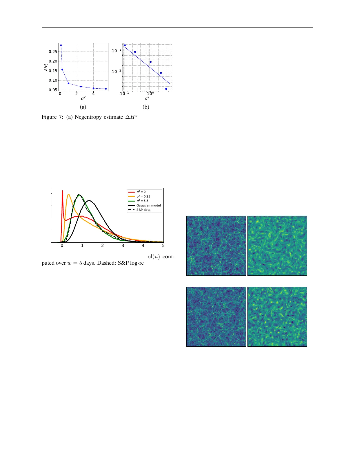
M G D : M O M E N T G U I D E D D I FF U S I O N F O R M A X I M U M E N T R O P Y G E N E R A T I O N A P R E P R I N T Etienne Lempereur 1 , Nathana ¨ el Cuvelle–Magar 1 , Florentin Coeurdoux 2 , St ´ ephane Mallat 3,4 , and Eric V anden-Eijnden 5,6 1 D ´ epartement d’informatique, ENS, Univ ersit ´ e PSL, Paris, France 2 Capital Fund Management, Paris, France 3 Coll ` ege de France, Paris, France 4 Flatiron Institute, New Y ork, USA 5 Courant Institute of Mathematical Sciences, New Y ork Uni versity , New Y ork, USA 6 ML Lab, Capital Fund Management, Paris, France February 20, 2026 A B S T R AC T Generating samples from limited information is a fundamental problem across scientiﬁc domains. Classical maximum entropy methods provide principled uncertainty quantiﬁcation from moment constraints but require sampling via MCMC or Langevin dynamics, which typically exhibit expo- nential slowdo wn in high dimensions. In contrast, generati ve models based on diffusion and ﬂow matching efﬁciently transport noise to data but offer limited theoretical guarantees and can overﬁt when data is scarce. W e introduce Moment Guided Diffusion (MGD), which combines elements of both approaches. Building on the stochastic interpolant frame work, MGD samples maximum entropy distributions by solving a stochastic dif ferential equation that guides moments to ward pre- scribed v alues in ﬁnite time, thereby av oiding slo w mixing in equilibrium-based methods. W e for - mally obtain, in the lar ge-volatility limit, con ver gence of MGD to the maximum entropy distrib ution and derive a tractable estimator of the resulting entropy computed directly from the dynamics. Ap- plications to ﬁnancial time series, turb ulent ﬂo ws, and cosmological ﬁelds using wa velet scattering moments yield estimates of negentropy for high-dimensional multiscale processes. 1 Introduction Generating ne w realizations of a random v ariable X ∈ R d from limited information arises across scientiﬁc domains, from synthesizing physical ﬁelds in computational sci- ence to creating scenarios for risk assessment in quantita- tiv e ﬁnance. Many approaches to this problem have been proposed, but two stand out for their success: the clas- sical maximum entropy framework introduced by Jaynes [1] when moment information is a vailable, and the mod- ern generativ e modelling approach with deep neural net- works [2 – 8] that operate when raw data samples can be accessed. These approaches take different perspecti ves on the problem—principled uncertainty quantiﬁcation versus ﬂexible distribution learning—suggesting potential bene- ﬁts from blending both. The maximum entropy approach provides principled un- certainty quantiﬁcation when the available information consists of moments E [ ϕ ( X )] ∈ R r for a speciﬁed mo- ment function (or observable) ϕ : R d → R r . Jaynes’ principle selects the unique distribution that maximizes entropy , if it exists. It is the least committal choice con- sistent with av ailable information. It provides principled protection against o verﬁtting: generated samples are di- verse within the constraint set but do not hallucinate corre- lations beyond what ϕ captures. This is particularly v alu- able when data is scarce. This maximum entropy distribu- tion has an exponential density p θ ∗ ( x ) = Z − 1 θ ∗ e − θ ∗ T ϕ ( x ) , where θ ∗ are Lagrange multipliers and Z θ ∗ is the normali- sation constant. While theoretically elegant and pro viding rigorous control over uncertainty , this approach is not a generativ e model per se . Classical maximum entrop y es- timation [9 – 11] requires sampling from intermediate dis- MGD: Moment Guided Diffusion for Maximum Entrop y Generation A P R E P R I N T tributions to compute log-likelihood gradients, both for estimating the Lagrange multipliers θ ∗ and for generat- ing samples from p θ ∗ . Unfortunately , samplers based on MCMC or on a Langevin equation suffer from critical slowing down [12, 13]: sampling becomes prohibiti vely expensi ve in high dimension for non-con vex Gibbs ener- gies θ T ∗ ϕ ( x ) . Recent generati ve modelling approaches emphasize ﬂexi- ble distribution learning when samples ( x i ) i ≤ n are avail- able. Modern generativ e models—notably score-based diffusion [6 – 8] and ﬂow matching with stochastic inter- polants [3, 4, 14]—learn to sample from an approxima- tion of the underlying distribution by transporting Gaus- sian noise to data samples along carefully designed paths using Ordinary Differential Equations (ODE) or Stochas- tic Differential Equations (SDE), with a drift estimated by quadratic regression with a neural network. This transport av oids the exponential scaling with barrier heights that plagues classical MCMC and Langevin sampling. Ho w- ev er , this ﬂexibility comes at a cost: they provide no ex- plicit control over statistical moments and their approxi- mation error remains theoretically uncontrolled, making them prone to ov erﬁtting when data is scarce [15]. W e introduce a Moment Guided Diffusion (MGD), which blends both paradigms. MGD samples maximum entrop y distributions when data samples are av ailable, using a transport that guides moments estimated from these data. T o achiev e this, MGD relies on two key ingredients. First, it uses a diffusi ve process X t whose moments match those of a stochastic interpolant I t that continuously transforms Gaussian noise into data: E [ ϕ ( X t )] = E [ ϕ ( I t )] for all t ∈ [0 , 1] . This dif fusion steers the distrib ution of the pro- cess from noise to data along a homotopic path, achie ving non-equilibrium transport in ﬁnite time and avoiding the critical slowing down that plagues classical Langevin dy- namics. Second, the SDE includes a tunable volatility σ that controls conv ergence to the maximum entropy dis- tribution. As σ increases, under appropriate assumptions we prove that the process conv erges to the maximum en- tropy among all distributions satisfying the moment con- straints. W e conjecture that this con vergence occurs at rate O ( σ − 2 ) , and provide numerical v eriﬁcation. MGD also enables estimation of the entrop y of the result- ing distribution. W e provide a tractable lower bound on the maximum entropy , computed directly from the MGD dynamics. W e conjecture and numerically validate that this lower bound con verges at rate O ( σ − 2 ) . This al- lows us to calculate the negentropy , which measures the non-Gaussianity of a random process as the difference between the entropy of a Gaussian with the same co- variance and the entropy of the process [16, 17]. Prior to this work, numerical computation of this information- theoretic measure was prohibitiv ely expensiv e for high- dimensional processes characterized by non-con vex ener - gies. The MGD SDE is a nonlinear (McKean-Vlasov) equa- tion whose drift depends on moments of its own solution. These moments are estimated empirically using interact- ing particles, and the dynamics is discretized in time. The computational cost scales as O ( σ 2 ) , with a constant inde- pendent of both the data dimension and the non-con vexity of the Gibbs energy . MGD is related to microcanonical sampling algo- rithms [18], which also generate samples in high dimen- sion without estimating Lagrange parameters. Ho wev er, the two methods dif fer in important ways. Microcanoni- cal algorithms transport a Gaussian distribution toward a distribution satisfying the moment constraints using a gra- dient descent on the moment mismatch, which requires inﬁnite time. Despite good numerical results in high di- mension [19 – 21], they are not guaranteed to conv erge to the maximum entropy distribution, nor can they estimate the maximum entropy value. MGD, by contrast, achieves ﬁnite-time transport along a homotopic path and pro vides a tractable entropy estimator . W e apply MGD to high-dimensional multiscale stochas- tic processes, generating ﬁnancial time-series and phys- ical ﬁelds from maximum entropy models conditioned by wavelet scattering moments [18, 21]. MGD pro- duces accurate models of complex non-Gaussian pro- cesses with long-range correlations, including ﬁnancial time series (S&P 500), turbulent ﬂo ws [22], and cosmo- logical ﬁelds [23]. F or these ﬁelds, we provide the ﬁrst estimates of negentropy . The remainder of this paper is organized as follows. Sec- tion 2 revie ws classical maximum entropy sampling via MCMC and Langevin dynamics, as well as modern gen- erativ e models based on dif fusion and stochastic inter- polants. Section 3 introduces the MGD transport and its numerical implementation. Section 4 presents the en- tropy estimator , discusses the con ver gence of MGD as the volatility increases, and states our conjectures on the con- ver gence rate. Section 5 provides numerical veriﬁcation of these conjectures. Section 6 applies MGD to high- dimensional multiscale processes—ﬁnancial time series, turbulent ﬂows, and cosmological ﬁelds—using wa velet scattering moments, and estimates their ne gentropy . T ech- nical proofs and additional details are provided in Ap- pendix. 2 Background: Classical Maximum Entropy and Moder n Generative Modeling W e revie w the classical sampling approach of maximum entropy distributions with Langevin dynamics (Section 2.1) and modern generati ve modeling based on transport via ﬂow matching and stochastic interpolants (Section 2.2). 2 MGD: Moment Guided Diffusion for Maximum Entrop y Generation A P R E P R I N T T able 1: Comparison of sampling approaches for complex distributions. Appr oach Input Max-ent guarantee Moment control Sampling Maximum entropy (classical) Moments m ✓ ✓ Equilibrium (MCMC) Diffusion models Dataset ( x i ) × × Non-equilibrium Moment Guided Diffusion Dataset ( x i ) ✓ ✓ Non-equilibrium (guided) 2.1 Maximum Entropy Estimation via Lange vin Dynamics Giv en a moment function ϕ : R d → R r with target ex- pectation m ∈ R r , the maximum entr opy principle seeks the probability density function (PDF) p which satisﬁes the moment constraints E p [ ϕ ] = Z ϕ ( x ) p ( x ) dx = m, (1) while maximizing the differential entrop y H ( p ) = − Z p ( x ) log p ( x ) dx. (2) Since inﬁnitely man y densities satisfy the moment con- straints, entropy maximization acts as a concave regular- ization that selects a unique solution. Introducing La- grange multipliers θ ∈ R r for these constraints, the La- grangian L ( p, θ ) = H ( p ) − θ ⊤  E p [ ϕ ] − m  (3) has, if a maximizer exists, a unique maximum at ( p ∗ , θ ∗ ) , where the maximum entropy density p ∗ = p θ ∗ takes the exponential form: p θ ( x ) = Z − 1 θ e − θ ⊤ ϕ ( x ) , with Z θ = Z R d e − θ ⊤ ϕ ( x ) dx. (4) The optimal parameter θ ∗ equiv alently maximizes L ( p θ , θ ) = − θ ⊤ m − log Z θ . While direct e valuation is in- tractable because it requires computing the normalisation constant Z θ , the gradient can be estimated by sampling from p θ , since ∇ θ L ( p θ , θ ) = E p θ  ϕ  − m, (5) because ∇ θ log Z θ = − E p θ  ϕ  . Sampling from p θ is typically performed using MCMC methods [24] based e.g. on Lange vin dynamics, i.e. via solution of the SDE dX t = − σ 2 θ ⊤ ∇ ϕ ( X t ) dt + √ 2 σ dW t , (6) where W t is a standard Brownian motion, σ is a volatil- ity parameter , and ∇ denotes the gradient with respect to x ∈ R d . Under suitable conditions, the law of X t con- ver ges to the distribution with density p θ as t → ∞ and, by ergodicity , E p θ [ ϕ ] can be estimated by a time av er- age along the trajectory . In practice, the SDE (6) is dis- cretized using an Euler -Maruyama scheme [25, 26], and a Metropolis-Hastings accept-reject step is added to correct for discretization bias—this is the Metropolis Adjusted Langevin Algorithm (MALA) [27]. Unfortunately , Lange vin dynamics and MCMC algo- rithms more generally suffer from critical slowing down for non-con vex energies, leading to prohibitiv ely long equilibration times. In particular , MALA scales poorly with dimension [28, 29], with sampling time gro wing ex- ponentially in most cases. This is particularly problematic for parameter estimation, since sampling must be repeated at each iteration of the optimization ov er θ to update E p θ [ ϕ ] as θ changes. The computational cost of both parameter estimation and sam- ple generation typically becomes impractical for high- dimensional distributions. When samples ( x i ) i ≤ n of p are a vailable, score match- ing [17] of fers an alternativ e approach to the estimation of θ ∗ . It av oids sampling p θ by minimizing the Fisher div ergence I ( p, p θ ) = E p  |∇ log p θ − ∇ log p | 2  . After integration by parts, the Fisher diver gence can be writ- ten, up to a constant, as an expectation ov er the data: I ( p, p θ ) = E p  |∇ log p θ | 2 + 2∆ log p θ  + cst , where ∆ denotes the Laplacian. The resulting score matching pa- rameter ˜ θ ∗ that minimizes the Fisher di vergence is a solu- tion of the linear system [17] E p  ∇ ϕ · ∇ ϕ ⊤  ˜ θ ∗ = E p  ∆ ϕ  . (7) The expectations in this equation can be estimated empir - ically using data samples ( x i ) i ≤ n , without sampling in- termediate distributions. It is therefore a much faster al- gorithm but ˜ θ ∗ = θ ∗ only if the data distribution already belongs to the exponential family , i.e., p = p θ ∗ . This condition is usually not satisﬁed. Moreover , if the Gibbs energy of p is non-con vex, this estimator has high vari- ance [30], making it unreliable. 2.2 Flow Matching with Stochastic Interpolants Since the seminal w ork of Ho, Song and collabora- tors [6, 7], complex data generation has been addressed by transporting samples between Gaussian white noise and a target distribution p , through re versal of a stochas- tic noising process. T ransport-based generative models hav e since been dev eloped under various names—ﬂow matching [3], stochastic interpolants [4], and rectiﬁed ﬂows [14]. These methods deﬁne time-dependent interpo- lations between two distributions and sample from them using ﬂows (ODEs) or diffusions (SDEs). W e adopt the stochastic interpolant formulation in what follows. A variance preserving stochastic interpolant I t between samples Z from a prior distribution (typically Gaussian noise, Z ∼ N (0 , Id) ) and data X ∼ p is deﬁned by I t = cos( α t ) Z + sin( α t ) X , t ∈ [0 , 1] , (8) 3 MGD: Moment Guided Diffusion for Maximum Entrop y Generation A P R E P R I N T where α t is a C 1 ([0 , 1]) function with boundary condi- tions α 0 = 0 and α 1 = π 2 (for example α t = π 2 t ), so that I 0 = Z and I 1 = X . The key observation made in [4, 5] is that the PDF p t ( x ) of the interpolant I t can be sampled via an SDE whose coef ﬁcients are estimable from data. Speciﬁcally , let X t satisfy the SDE dX t = b t ( X t ) dt + σ 2 ∇ log p t ( X t ) dt + √ 2 σ dW t , (9) where W t is a Bro wnian noise and σ ≥ 0 is a tunable volatility with b t ( x ) = E  ˙ I t | I t = x  , (10) where the dot denoting the time deri vati ve and E  · | I t = x  the expectation over the law of I t conditional on I t = x . Then, if X 0 = I 0 = Z , X t and I t share the same PDF p t for all t ∈ [0 , 1] . By Stein’ s formula, the score ∇ log p t can also be expressed as a conditional e xpectation: ∇ log p t ( x ) = − 1 cos( α t ) E  Z | I t = x  . (11) Since a conditional expectation is the minimizer of a quadratic loss, b t and ∇ log p t can be learned by minimis- ing this loss, typically by representing them in a rich para- metric class such as a deep neural network. Unlike the Langevin SDE (6), which follows equilibrium dynamics whose law con verges to p θ only as t → ∞ , the SDE (9) deﬁnes a non-equilibrium transport that reaches the target distribution at time t = 1 . Crucially , this transport avoids the critical slo wing down that plagues Langevin dynamics. Because the interpolant I t mixes data with Gaussian noise, the distrib ution p t varies smoothly from a simple Gaussian at t = 0 to the target at t = 1 . Par - ticles follo wing the SDE (9) are guided along this smooth path, with the complex structure of the tar get emerging gradually as t → 1 . For example, in multimodal distri- butions, particles are positioned inside the correct modes early (when the landscape is smooth) and remain there as the modes sharpen. W e illustrate this in Figure 1. Stochastic interpolants thus provide a fast sampler that ap- proximates the data distribution. In theory , the drift b t re- produces the full density p t of I t at each time, and hence the target density p at t = 1 . W ith sufﬁcient training data, deep neural networks generalize well on complex datasets [15]. It results from an implicit regularization produced by the stochastic gradient descent of the neural network optimization [31, 32], which is not well under- stood. In the lo w-data regime, howe ver , the learned model may overﬁt and memorize the training samples. Max- imum entropy models offer a complementary approach: they pro vide explicit regularization through entropy max- imization, leading to analytic exponential distributions with controlled approximation error . The next section shows that they can also be sampled via stochastic inter- polation. 0.0 0.2 0.4 0.6 0.8 1.0 t 2 0 2 4 Z ( 0 , 1 ) X Figure 1: Illustration of trajectories ( in blue or red) of X t satisfying Equation (9) for an interpolant I t deﬁned with α t = π t/ 2 between white noise Z and a bimodal unbalanced Gaussian mixture X , for σ = 1 . W e display in gray in the background the density of I t . When t goes to 0 , the modes progressively disappear . At early times t , particles evolv e freely in space, but they become trapped in the modes when the density p t becomes bimodal. Red particles are conﬁned in the upper mode and blues in the lower one. 3 Moment Guided Diffusion In this section, we introduce Moment Guided Dif fusion (MGD), which guides moments exactly along an interpo- lation path while injecting Langevin noise. W e show that this preserves moments at each time; conv ergence to the maximum entropy distribution as the v olatility increases will be discussed in Section 4. Section 3.1 deﬁnes the MGD SDE and establishes conditions under which it pre- serves moments. Section 3.2 introduces a discretized al- gorithm and discusses its numerical cost. 3.1 Moment Guided Diffusion A stochastic interpolant SDE (9) produces X t with the same distribution as I t , thereby reproducing all moments. MGD uses the same interpolant I t , but imposes only that a ﬁnite number of moments is preserved: ∀ t ∈ [0 , 1] : E  ϕ ( X t )  = E  ϕ ( I t )  := def m t . (12) The following theorem shows that this weaker constraint is satisﬁed by an SDE formally similar to the Langevin equation (6), but with a time-dependent drift analogous to (10). Theorem 3.1 (Moment Guided Diffusion) . Consider the SDE dX t =  η ⊤ t − σ 2 θ ⊤ t  ∇ ϕ ( X t ) dt + √ 2 σ dW t , X 0 = Z, (13) wher e W t is a Br ownian noise and η t and θ t solve G t η t = d dt m t , (14) G t θ t = E  ∆ ϕ ( X t )  , (15) wher e G t is the Gram matrix G t = E  ∇ ϕ ( X t ) · ∇ ϕ ( X t ) ⊤  . (16) 4 MGD: Moment Guided Diffusion for Maximum Entrop y Generation A P R E P R I N T If this coupled system admits a solution, then the moment condition E  ϕ ( X t )  = m t holds for all t ∈ [0 , 1] . The proof of Theorem 3.1 is given in Appendix A. By applying It ¯ o’ s lemma, we sho w that any solution satisﬁes ∀ t ∈ [0 , 1] : d dt E  ϕ ( X t )  = d dt m t , (17) which implies E [ ϕ ( X t )] = m t since this holds at t = 0 . Note that the e xistence of a solution needs to be assumed. Since G t , η t , and θ t depend on the law of X t , (13) is a nonlinear (McKean-Vlaso v) SDE [33, 34] whose well- posedness is non-trivial. In particular, G t may become singular , causing the drift to blo w up. Sufﬁcient condi- tions for existence are established in Appendix F: Theo- rem F .7 prov es that for large enough σ , a version of MGD with an additional conﬁning potential admits strong solu- tions X t that conv erge to the maximum entropy distribu- tion with moments m t . The proof relies on the assumption that the Poincar ´ e constant of a reference measure is ﬁnite. If p 0 is Gaussian and ϕ ( x ) = ( x, xx ⊤ ) , then MGD so- lutions exist and are independent of σ . In particular , one may set σ = 0 , reducing the SDE (13) to an ODE. Ap- pendix E shows that under these hypotheses, X t is Gaus- sian with the same mean and covariance as I t , so MGD exactly samples the maximum entropy distribution for all σ ≥ 0 . Remark 3.2 (Sampling vs. modelling error) . Thr ough- out this paper , “exact sampling” refers to sampling fr om the maximum entr opy distribution p ∗ constrained by E p ∗ [ ϕ ] = E [ ϕ ( X )] , not fr om the true data distribution p . The discrepancy D KL ( p ∥ p ∗ ) reﬂects model misspeciﬁca- tion inher ent to the choice of moment function ϕ , and is distinct fr om the sampling err or D KL ( p σ 1 ∥ p ∗ ) that MGD contr ols (if p σ 1 is the density of X 1 ). F or general ϕ , the dynamics at σ = 0 typically does not yield the distribution of X 1 to be the maximum entr opy distribution with moments E [ ϕ ( X )] . The volatility σ con- tr ols con vergence to maximum entr opy: Br ownian noise incr eases entr opy , while the guidance η t can reduce it. When σ is lar ge, the noise dominates. W e conjectur e (Sec- tion 4) and verify numerically (Section 5) that p σ 1 → p ∗ as σ → ∞ . It means that MGD eliminates the sampling err or while the modelling err or remains a choice dictated by ϕ . T urning now to the structure of the MGD SDE, the drift in (13) has two components: η t steers the process to ad- just the target moments m t to m t + dt , while σ 2 θ t counter- balances the moment modiﬁcation induced by the added white noise σ dW t . Note that the MGD SDE (13) is struc- turally similar to the stochastic interpolant SDE (9): it has a transport term proportional to η t (analogous to b t ) and a score-like term proportional to θ t (analogous to ∇ log p t ). In particular , θ t solves an equation of the same form as the score matching equation (7), but with expectations taken ov er the law of X t rather than the data distribution p . As with stochastic interpolants (Section 2.2), MGD de- ﬁnes a non-equilibrium homotopic transport that reaches the target moments at t = 1 , see Section 4.1 for more discussion. W e stress, howe ver , that θ ⊤ t ∇ ϕ ( x ) is not the score of the PDF of X t . Unlike the stochastic interpolant SDE, where the score term is exact, the MGD drift does not reproduce the full distribution of I t but only its mo- ments E [ ϕ ( I t )] . This is the key dif ference between MGD and stochastic interpolants. Remark 3.3. Observe that θ 1 in (15) coincides with the scor e matching parameter in (7) computed for X 1 . If the distribution of X 1 con ver ges to p ∗ as σ → ∞ , then θ 1 con ver ges to θ ∗ . A ﬁnite sample estimator of θ 1 is thus a nearly consistent estimator of θ ∗ for lar ge σ . However , as noted in Section 2, scor e matching estimators have high variance for non-con vex ener gies. Crucially , MGD’ s sam- pling accuracy depends on the empirical estimation of m t , not on the accuracy of θ t (see Section 5.2.) 3.2 Discretization of MGD W e solve numerically the MGD nonlinear (McKean- Vlasov) SDE (13) by iterativ ely updating a ﬁnite ensem- ble of interacting particles. T o update the particles, we estimate η t in (14) and θ t in (15) with empirical means ov er these particles. W e also av oids computing E [∆ ϕ ] , which is costly or ill-deﬁned when ϕ is not smooth. This is achieved with a two-step predictor-corrector scheme, which we ﬁrst describe using exact expectations before discussing ﬁnite-particle estimations. Giv en X t and some small time step h > 0 , let Y be ob- tained via Y = X t + h η T t ∇ ϕ ( X t ) + √ 2 σ ( W t + h − W t ) , (18) with η t the solution to (14). This is the Euler-Maruyama scheme for the MGD SDE (13) with θ t = 0 . As such, the update (18) does not preserve the moments, i.e. E [ ϕ ( Y )]  = m t + h . W e enforce this moment condition by adding to Y a term similar to the one in volving θ t in the MGD SDE (13), i.e. setting X t + h = Y − h σ 2 ˆ θ ⊤ ∇ ϕ ( Y ) , (19) and requiring that E  ϕ ( X t + h )  = m t + h . (20) Substituting (19) into (20) giv es an equation for ˆ θ . Solv- ing this exactly is costly (it is nonlinear in ˆ θ ) and unneces- sary , since the Euler-Maruyama update is only accurate to weak order 1 in h . W orking to the same order of accuracy , we T aylor expand the left-hand side of (20) to obtain hσ 2 E  ∇ ϕ ( Y ) · ∇ ϕ ( Y ) ⊤  ˆ θ = E  ϕ ( Y )  − m t + h . (21) Since E  ϕ ( X t )  = m t , the right-hand side equals h E  ∆ ϕ ( X t )  + o ( h ) , so to leading order (21) reduces to (15) and ˆ θ = θ t . In the numerical scheme, how- ev er , it is more con venient to solv e (21) directly since this av oids computing E [∆ ϕ ( X t )] . This is important when ϕ includes ℓ 1 norms or absolute values, for which ∆ ϕ is a 5 MGD: Moment Guided Diffusion for Maximum Entrop y Generation A P R E P R I N T sum of Dirac functions whose expectation is hard to esti- mate unless the number of samples is very lar ge. T o turn this into a practical scheme, we need to choose the time step h . Since the drift is proportional to σ 2 for large σ , so is its Lipschitz constant. W e therefore set the num- ber of steps to n σ = aσ 2 + b , where b ensures the limiting ODE ( σ → 0 ) is accurately solv ed. The computational cost of MGD thus scales as O ( σ 2 ) . The scheme is summarized in Algorithm 1. It iterativ ely ev olves a population of n rep particles ( x i k ) 1 ≤ i ≤ n rep (repli- cas), whose empirical measure approximates the distrib u- tion of X k/n σ , using moments m t estimated from training data. A k ey property is that the moment condition (20) re- mains v alid when expectations are replaced by empirical av erages o ver particles, since (21) holds for empirical dis- tributions. As a result, the empirical mean of ϕ over the particles conv erges to m t + h as the step size h → 0 . This exact moment tracking controls the dynamical stability of the algorithm: a di vergence of particles would manifest as a moment mismatch (see Remark 3.3). Alternativ e imple- mentations are discussed Appendix C and some numerical details in Appendix D. Algorithm 1 Moment-Guided Diffusion (MGD) Input: volatility σ ; number of steps n σ = O ( σ 2 ) ; time step h = 1 /n σ ; number of replicas n rep ; moments m t = E [ ϕ ( I t )] Initialize: x i 0 ∼ N (0 , Id) for i = 1 , . . . , n rep Pr edictor for k = 0 , . . . , n σ − 1 do Compute ˆ G k = 1 n rep P n rep i =1 ∇ ϕ ( x i k ) · ∇ ϕ ( x i k ) ⊤ Solve ˆ G k ˆ η k = d dt m kh for ˆ η k for i = 1 , . . . , n rep do Sample ξ i k ∼ N (0 , Id) Set y i k = x i k + h ˆ η ⊤ k ∇ ϕ ( x i k ) + √ 2 hσ ξ i k end for Corr ector (pr oject to preserve moments) Compute ˆ G ′ k = 1 n rep P n rep i =1 ∇ ϕ ( y i k ) · ∇ ϕ ( y i k ) ⊤ Solve hσ 2 ˆ G ′ k ˆ θ k = 1 n rep P n rep i =1 ϕ ( y i k ) − m ( k +1) h for ˆ θ k for i = 1 , . . . , n rep do Set x i k +1 = y i k + h ˆ θ ⊤ k ∇ ϕ ( y i k ) end for end for Output: Samples ( x i n σ ) 1 ≤ i ≤ n rep 4 Maximum Entropy: Con vergence and Bounds Let p σ t be the PDF of the solution X t of the MGD SDE (13) for a volatility σ . Section 4.1 studies the con- ver gence of p σ 1 tow ards the maximum entropy distribution p ∗ . Section 4.2 computes a tractable lower bound of the entropy H ( p σ 1 ) and conjectures its con ver gence to wards H ( p ∗ ) when σ increases. 4.1 Con vergence towards the Maximum Entr opy Distribution A central claim of this paper is that, as σ → ∞ , the distri- bution p σ 1 of the MGD output conv erges to the maximum entropy distribution p ∗ . Next, we provide heuristic sup- port for this claim via a formal T aylor expansion, then state it precisely as Conjecture 4.1. The conjecture is ver - iﬁed numerically in Section 5. The time ev olution of the PDF p σ t of the solution of the MGD SDE (13) is gov erned by the Fokker -Planck equa- tion: ∂ t p σ t = ∇ · ( p σ t (( − η t + σ 2 θ t ) ⊤ ∇ ϕ )) + σ 2 ∆ p σ t . (22) Formally taking σ → ∞ and keeping only the leading- order terms, the Fokker -Planck equation reduces to ∇ · ( p ∗ t ( θ ∗ t ⊤ ∇ ϕ )) + ∆ p ∗ t = 0 , (23) where p ∗ t and θ ∗ t denote the (formal) limits of p σ t and θ t as σ → ∞ . The solution of this limit equation is an e xpo- nential distribution: p ∗ t = ( Z ∗ t ) − 1 e − θ ∗ t ⊤ ϕ , (24) with normalising constant Z ∗ t . This suggests that p σ t con- ver ges to an exponential distrib ution with moments m t , and hence to the maximum entrop y distribution satisfying these constraints. In particular , this giv es p ∗ 1 = p ∗ and θ ∗ 1 = θ ∗ . Expanding p σ t = p ∗ t (1 + q t σ − 2 + o ( σ − 2 )) , for some q t that does not depend upon σ , Appendix B provides a formal calculation showing that the Kullback- Leibler diver gence satisﬁes D KL ( p σ 1 ∥ p ∗ ) = O ( σ − 2 ) . This leads to the following conjecture: Conjecture 4.1 (Max entropy) . Ther e exists C > 0 such that for all σ > 0 D KL ( p σ 1 ∥ p ∗ ) ≤ C σ − 2 . (25) A numerical veriﬁcation is giv en in Section 5. Since p σ 1 and p ∗ share the same moments, we hav e D KL ( p σ 1 ∥ p ∗ ) = H ( p ∗ ) − H ( p σ 1 ) , (26) so (25) is equiv alent to H ( p ∗ ) − H ( p σ 1 ) ≤ C σ − 2 . (27) Remark 4.2. In numerical experiments, we choose p 0 to be a Gaussian PDF . If ϕ is quadr atic ( ϕ ( x ) = xx ⊤ ) since ∇ ϕ ( x ) is linear , dX t in the MGD (22) is the sum of two Gaussian random vector s so X t r emains Gaussian for all t with second order moments equal to m t . It results that p σ t is Gaussian with the same mean and co variance as I t , and does not depend on σ . More generally , Theor em E.1 in Appendix E pr oves that for any sufﬁciently r egular p 0 , if ϕ ( x ) = ( x, xx ⊤ ) , then MGD admits str ong solutions and lim σ →∞ D KL ( p σ 1 ∥ p ∗ ) = 0 . 6 MGD: Moment Guided Diffusion for Maximum Entrop y Generation A P R E P R I N T Since the numerical cost of MGD is O ( σ 2 ) (see Section 3.2), the cost required to reach a given error is propor- tional to the constant C appearing in Conjecture 4.1. This constant depends on the moment function ϕ and the mo- ments m t , and becomes large when ϕ is not expressi ve enough to capture the homotopic transport of mass at early times t —before the maximum entropy distribution with moments m t becomes multimodal. If x ∈ R , a truncated monomial basis ϕ ( x ) = ( x k ) k ≤ r provides this ﬂexibility , as illustrated in Section 5.1. If x ∈ R d , since the number of monomials grows polyno- mially with d , this strategy becomes computationally pro- hibitiv e for d lar ge. A wa velet scattering spectra ϕ [21] computes O (log 3 d ) low-order multiscale moments that are similar to fourth order moments. In Section 6, we show that for real-world high-dimensional datasets from physics and ﬁnance, it is suf ﬁcient rich to capture this ho- motopic transport with a small C . Modelling the transport of mass does not require ϕ to pro- vide an accurate model the full distrib ution of I t . W e sho w in Section 6.5 that C can be small although the model mis- speciﬁcation D KL ( p ∥ p ∗ ) is lar ge. 4.2 Entropy Estimation W e now compute a tractable lower bound on the en- tropy H ( p σ 1 ) and conjecture that it con verges to H ( p ∗ ) as σ → ∞ . Proposition 4.3. Assume the MGD SDE (13) admits a unique str ong solution for all t ∈ [0 , 1] . Then, d dt H ( p σ t ) = θ ⊤ t d dt m t + σ 2 E  |∇ log p σ t ( X t ) + θ ⊤ t ∇ ϕ ( X t ) | 2  , (28) and hence d dt H ( p σ t ) ≥ θ ⊤ t d dt m t . (29) The proof, gi ven in Appendix A, uses the Fokker-Planck equation (22) to compute the ev olution of the differential entropy of p σ t . When the moments are constant ( d dt m t = 0 ), the entrop y increases along the dynamics. In this case, H ( p σ t ) also increases with σ , as shown by a time-rescaling argument in Proposition A.1. Sections 5 and 6 provide nu- merical veriﬁcation that d dσ H ( p σ t ) ≥ 0 more generally . Integrating (29) ov er [0 , 1] yields a lower bound on the entropy of the sampled distrib ution p σ 1 : H ( p σ 1 ) ≥ H σ ∗ := def H ( p 0 ) + Z 1 0 θ ⊤ t d dt m t dt. (30) This lower bound can be computed directly from the MGD parameters along the dynamics. From (28), the g ap between H ( p σ 1 ) and its lo wer bound is H ( p σ 1 ) − H σ ∗ = σ 2 Z 1 0 E  |∇ log p σ t ( X t )+ θ ⊤ t ∇ ϕ ( X t ) | 2  dt. (31) This integral is the time-av eraged Fisher diver gence be- tween p σ t and the exponential distribution with energy θ ⊤ t ϕ . If Conjecture 4.1 holds, this Fisher diver gence van- ishes as σ → ∞ , pro vided that p 0 itself has an exponential form. In particular , this holds when X 0 = Z is Gaussian and ϕ includes quadratic terms so that θ ⊤ 0 ϕ ( x ) = | x | 2 / 2 for some θ 0 . The lower bound H σ ∗ then con ver ges to wards H ( p ∗ ) . Conjecture 4.4 (Entropy bound) . If Z has density p 0 = Z − 1 0 e − θ ⊤ 0 ϕ , then ther e exists C > 0 such that for all σ > 0 , H ( p ∗ ) − H σ ∗ ≤ C σ − 2 . (32) Supporting arguments from the same Fokker –Planck anal- ysis are given in Appendix B, with numerical veriﬁcation in Section 5. In practice, monitoring the con ver gence of H σ ∗ provides a diagnostic for the con ver gence of p σ 1 to p ∗ . 5 Numerical V alidation Section 5.1 studies the numerical con vergence proper- ties of Moment Guided Diffusions to wards maximum en- tropy distributions, ov er distributions of one-dimensional x ∈ R . W e use a cosine interpolant deﬁned by I t = cos( 1 2 π t ) Z + sin( 1 2 π t ) X and solve the MGD SDE (13) with the numerical inte gra- tor speciﬁed in Section 3.2. Section 5.2 shows empirically that the numerical complexity of the MGD sampling does not suffer from the non-con vexity of the distributions as opposed to an MCMC sampling algorithm. 5.1 Con vergence towards Maximum Entr opy Distributions The MGD algorithm samples a distribution with density p σ 1 . W e study its numerical conv ergence to the maximum entropy distribution p ∗ ( x ) = Z − 1 θ ∗ e − θ ⊤ ∗ ϕ ( x ) and verify Conjectures 4.1 and 4.4 for different choices of data dis- tributions and moment functions ϕ . 5.1.1 Non-log-concav e Density W e consider data X ∼ p distributed according to an un- balanced bimodal density p ( x ) = Z − 1 e − 4 5 ( x 4 − 5 x 2 − x/ 2) for x ∈ R , and the four-dimensional monomial map ϕ ( x ) = ( x, x 2 , x 3 , x 4 ) , whose moments are E [ ϕ ( X )] ≈ (0 . 8 , 2 . 4 , 2 . 2 , 6 . 4) . With this choice, the maximum en- tropy density satisﬁes p ∗ ( x ) = p ( x ) . (Note that I t for t ∈ (0 , 1) is not distrib uted according to the maximum entropy distrib ution with moments m t .) The log-density log p ∗ ( x ) (dotted line) in Figure 2(a) ex- hibits two modes, reﬂecting a non-conv ex Gibbs energy . For small σ , the density p σ 1 concentrates in two separate modes. Although these modes do not hav e the correct shape (they are too peaked, reﬂecting the lack of entropy of p σ 1 ), their relati ve weight is correct. As σ increases, the added noise allo ws particles to spread correctly inside the 7 MGD: Moment Guided Diffusion for Maximum Entrop y Generation A P R E P R I N T modes, and p σ 1 progressiv ely conv erges tow ards p ∗ , with near-superposition at σ 2 = 5 . Figure 2(b) quantiﬁes this con vergence via the entropy H ( p σ 1 ) (blue), computed numerically from the distribu- tions above. These values lie below H ( p ∗ ) = 0 . 67 (red). W e observe that d dσ H ( p σ 1 ) ≥ 0 and that H ( p σ 1 ) → H ( p ∗ ) as σ 2 increases. Figure 2(c) shows D KL ( p σ 1 ∥ p ∗ ) = H ( p ∗ ) − H ( p σ 1 ) (blue dots), which decays as O ( σ − 2 ) on the log-log scale (black dashed line shows σ − 2 decay), validating Conjecture 4.1. The lower bound H σ ∗ on H ( p σ 1 ) , computed from (30), is shown as black dots in Figure 2(b). As expected, it lies below H ( p σ 1 ) (blue) and also con ver ges to H ( p ∗ ) . Fig- ure 2(c) sho ws that H ( p ∗ ) − H σ ∗ (black dots) also decays as O ( σ − 2 ) , validating Conjecture 4.4. 2 0 2 4 6 1 0 3 1 0 2 1 0 1 1 0 0 2 = 0 2 = 0 . 5 2 = 1 2 = 5 2 0 2 4 6 1 0 3 1 0 2 1 0 1 1 0 0 2 = 0 2 = 5 0 2 = 1 0 0 2 = 5 0 0 (a) (d) 1 0 0 1 0 1 2 0.2 0.4 0.6 H ( p * ) H ( p 1 ) H * 1 0 1 1 0 2 2 0.2 0.4 0.6 (b) (e) 1 0 0 1 0 1 2 1 0 2 1 0 1 1 0 0 H ( p * ) H * H ( p * ) H ( p 1 ) 1 0 1 1 0 2 2 1 0 2 1 0 1 1 0 0 (c) (f) Figure 2: Con vergence of MGD towards the maximum entropy bimodal distribution p ∗ ( x ) = Z − 1 e − 4 5 ( x 4 − 5 x 2 − x/ 2) for X ∼ p = p ∗ . Left column: moment function ϕ ( x ) = ( x, x 2 , x 3 , x 4 ) . Right column: ϕ ( x ) = ( x 2 , log p ( x )) . (a,d) Log-density log p ∗ ( x ) (dashed) and log p σ 1 ( x ) for increasing σ (blue to red). (b,e) Maximum entropy H ( p ∗ ) (red line), sampled en- tropy H ( p σ 1 ) (blue dots), and lower bound H σ ∗ from (30) (black dots) v ersus σ 2 . (c,f) Entropy gaps H ( p ∗ ) − H ( p σ 1 ) (blue) and H ( p ∗ ) − H σ ∗ (black) versus σ 2 ; the dashed line shows σ − 2 decay . 5.1.2 Slower Con vergence In the pre vious example, p σ 1 con verges towards p ∗ with negligible error for σ 2 ≥ 2 . W e now sho w that the con- ver gence constant C in Conjecture 4.1 depends critically on the choice of moment functions ϕ . When p is known, a seemingly natural choice is ϕ ( x ) = ( x 2 , log p ( x )) , since this sufﬁces to represent both the data density p and the initial Gaussian density p 0 , yield- ing p ∗ ( x ) = p ( x ) . F or the bimodal density p ( x ) = Z − 1 e − 4 5 ( x 4 − 5 x 2 − x/ 2) with this ϕ , Figures 2(e) and (f) conﬁrm that D KL ( p σ 1 ∥ p ∗ ) and H ( p ∗ ) − H σ ∗ both decay as C σ − 2 for σ 2 ≥ 50 , validating Conjectures 4.1 and 4.4. Howe ver , the constant C is much larger than in the previ- ous example: small errors require σ 2 ≥ 500 , or approxi- mately 10 2 times more integration steps. Figure 2(d) sho ws the densities p σ 1 for se veral v alues of σ . Although p σ 1 is bimodal for σ 2 ≤ 1 , the relativ e weights of the two modes are of f by one order of magnitude. This oc- curs because ϕ is not expressiv e enough to displace mass at early times t of the MGD, before p σ t becomes multi- modal. For larger values of σ 2 (abov e 10 2 ), MGD be- comes analogous to a Langevin dynamic, recov ering the correct relati ve weights through random switching of par - ticles between modes. 5 0 5 1 0 3 1 0 2 1 0 1 1 0 0 2 = 0 . 0 1 2 = 0 . 1 2 = 1 . 0 2 = 1 0 . 0 1.0 1.5 H ( p * ) H ( p 1 ) H * 1 0 1 1 0 0 1 0 1 2 1 0 3 1 0 1 1 0 1 H ( p * ) H * H ( p * ) H ( p 1 ) (a) (b) Figure 3: Con vergence of MGD tow ards the Laplacian maximum entropy distribution p ∗ ( x ) = 1 2 e −| x | for X ∼ p = p ∗ . (a) Log-density log p ∗ ( x ) (dashed) and log p σ 1 ( x ) for increasing σ (blue to red). (b, top) Maximum entropy H ( p ∗ ) (red line), sampled entropy H ( p σ 1 ) (blue dots), and lower bound H σ ∗ from (30) (black dots) versus σ 2 . (b, bot- tom) Entropy gaps H ( p ∗ ) − H ( p σ 1 ) (blue) and H ( p ∗ ) − H σ ∗ (black) versus σ 2 ; the dashed line shows σ − 2 decay . 5.1.3 Non-smooth ϕ The MGD numerical scheme (Section 3.2) av oids com- puting ∆ ϕ , which is essential when ϕ includes modulus or ℓ 1 norms, as in the scattering spectra of Section 6. W e v er- ify here that MGD correctly samples maximum entropy distributions deﬁned by non-smooth ϕ , and that Conjec- tures 4.1 and 4.4 hold. W e consider data distrib uted according to the Laplacian density p ( x ) = 1 2 e −| x | , which is the maximum entropy 8 MGD: Moment Guided Diffusion for Maximum Entrop y Generation A P R E P R I N T distribution p = p ∗ for ϕ ( x ) = ( x 2 , | x | ) with E [ ϕ ( X )] = (2 , 1) . Figure 3(a) shows log p σ 1 ( x ) for various σ . As σ in- creases, the curv es con verge to log p ∗ ( x ) (dashed), nearly superimposing at σ 2 = 10 . For small σ , the density p σ 1 ex- hibits a sharper spike near zero and shorter tails, reﬂecting insufﬁcient entrop y . Con vergence is quantiﬁed by D KL ( p σ 1 ∥ p ∗ ) = H ( p ∗ ) − H ( p σ 1 ) , which decreases to zero as σ 2 increases (Fig- ure 3(b, top)). Figure 3(b, bottom) conﬁrms H ( p ∗ ) − H ( p σ 1 ) = O ( σ − 2 ) for σ 2 ≥ 10 − 2 , v alidating Conjec- ture 4.1. The lower bound H σ ∗ from (30) (black dots) also con verges to H ( p ∗ ) at the same rate, v alidating Conjec- ture 4.4. Since the Laplacian is log-concave: there is no mass to displace between wells, so even a Langevin dy- namic would con ver ge quickly . 5.2 Rate of Con vergence and Multimodality W e verify numerically that the computational cost of MGD does not depend on energy barrier heights, unlike MCMC methods. W e use truncated monomial moment generating functions ϕ ( x ) = ( x k ) k ≤ r (for r = 4 ) 2 0 2 4 1 0 6 1 0 5 1 0 4 1 0 3 1 0 2 1 0 1 1 0 0 = 0.3 = 0.7 = 1.1 = 1.5 = 1.9 0.5 1.0 1.5 1 0 2 1 0 3 1 0 4 1 0 5 1 0 6 n s t e p s MGD MAL A (a) (b) Figure 4: (a) Log-density log p ∗ ( x ) for p ∗ ( x ) = Z − 1 β e − β ( x 4 − 5 x 2 − x/ 2) with increasing β (blue to red). The two modes are separated by a barrier of height propor- tional to β . (b) Number of discretization steps n steps re- quired to reach a ﬁxed K ullback–Leibler diver gence from p ∗ , for MALA (red) and MGD (green), as a function of β . For MALA, n steps grows exponentially with β ; for MGD, it remains nearly constant. Figure 4(a) shows the log-density of unbalanced bimodal distributions p ∗ ( x ) = Z − 1 β e − β ( x 4 − 5 x 2 − x/ 2) , with two modes separated by a barrier of height propor- tional to β . For MGD, we consider for simplicity that X is distrib uted according to the maximum entropy distrib u- tion p = p ∗ . The computational cost of both MGD and the Metropolis Adjusted Langevin Algorithm (MALA) is proportional to the number n steps of discretization steps. The cost per step differs between algorithms (typically higher for MGD), but it does not depend on β so we do take it into account. MALA computes samples via discretized Langevin dy- namics initialized from Gaussian white noise, with an accept-reject operation which eliminates the discretiza- tion bias. The step size is tuned to achieve an optimal ac- ceptance rate approximately 0 . 57 [35]. Although the sam- pled distribution ˜ p con verges to p ∗ as n steps increases, this con vergence depends exponentially on β . Indeed, cross- ing an energy barrier by adding Gaussian noise has prob- ability exponentially small in the barrier height. W e measure the minimum number of steps n steps required to reach a ﬁxed error D KL ( ˜ p ∥ p ∗ ) = 10 − 3 . Figure 4(b) conﬁrms that for MALA (red), n steps grows exponentially with β , making it computationally prohibitiv e for non- con vex distrib utions—especially in higher dimensions. For MGD, we know that n steps = n σ = O ( σ 2 ) and D KL ( p σ 1 ∥ p ∗ ) = O ( σ − 2 ) . W e choose σ so that the dis- cretized MGD satisﬁes D KL ( ˜ p σ 1 ∥ p ∗ ) = 10 − 3 . W e run this experiment for the moment generating function ϕ ( x ) = ( x, x 2 , x 3 , x 4 ) . Figure 4(b) shows that for MGD (green), n steps remains approximately constant as β increases. It veriﬁes that the MGD computational cost does not suffer from multimodality . The homotopic transport (Section 4.1) is able to distribute samples into correct modes early , enabling efﬁcient sam- pling. Ho wever , this property requires ϕ to be sufﬁ- cient rich to capture the mass transport at early times; for ϕ ( x ) = ( x 2 , log p ( x )) , MGD would rev ert to MCMC-like behavior . 6 Generation of Multiscale Processes in Finance and Physics This section applies the MGD algorithm to sample high- dimensional maximum entropy distributions. Section 6.2 revie ws multiscale maximum entropy models based on wa velet scattering moments. W e consider ﬁnancial time series (Section 6.3) as well as two-dimensional turbulent and cosmological ﬁelds (Section 6.2). T o v alidate Conjec- tures 4.1 and 4.4, we compute the lower bound of the en- tropy of sampled distributions, and study its con vergence as the v olatility σ increases. W e also estimate negentropy , which quantiﬁes order and non-Gaussianity (Section 6.1). Finally , we show numerically in Section 6.5 that the con- ver gence of MGD to the maximum entropy distrib ution p ∗ does not depend upon the model error D KL ( p ∥ p ∗ ) . 6.1 Negentropy Rate The negentrop y was introduced in statistical physics by Erwin Schr ¨ odinger [16] to measure the distance of sys- tem to equilibrium, and gi ve a measure of order and infor - mation. The negentropy usually can not be measured for high-dimensional systems because estimating the entropy is generally untractable. The negentropy of a random vector X is deﬁned as the difference between the entropy H ( p ) of the density p of X and the entropy H ( g ) of the gaussian density g hav- ing the same covariance Σ as p . The negentropy rate is 9 MGD: Moment Guided Diffusion for Maximum Entrop y Generation A P R E P R I N T normalised by the dimension d of X and can be rewrit- ten as the Kullback Leibler diver gence between p and the Gaussian g : ∆ H ( p ) = d − 1 ( H ( g ) − H ( p )) = d − 1 D KL ( p ∥ g ) ≥ 0 , (33) where the Gaussian entropy is gi ven by H ( g ) = d 2 log  2 π e (detΣ) 1 /d  . (34) The ne gentropy rate con verges when d goes to inﬁnity for extensi ve processes for which the entropy rate d − 1 H ( p ) con verges. It is in variant to the action of an in vertible lin- ear operator on X and hence does not depend upon the cov ariance of X , if it is inv ertible. In that sense it is an intrinsic measure of non-Gaussian properties of X . If p ∗ is the maximum entropy distribution conditioned by the moment value E p ( ϕ ) then H ( p ∗ ) ≥ H ( p ) and H ( p ∗ ) − H ( p ) = D KL ( p ∥ p ∗ ) and, as a result, ∆ H ( p ) = d − 1  H ( g ) − H ( p ∗ ) + D KL ( p ∥ p ∗ )  . (35) This implies that d − 1  H ( g ) − H ( p ∗ )  is a lower bound of the negentropy ∆ H ( p ) of p , which depends upon the accuracy of the maximum entropy model p ∗ deﬁned by D KL ( p ∥ p ∗ ) . The following sections give an estimate of this negentropy rate with the MGD algorithm, by com- puting the lower bound H σ ∗ in (30) of H ( p ∗ ) , and ∆ H σ ∗ = d − 1  H ( g ) − H σ ∗  . (36) The con ver gence of H σ ∗ when σ increases is equi valent to the con vergence of ∆ H σ ∗ . In particular , Conjecture 4.4 states that ∆ H σ ∗ should con verge at rate O ( σ − 2 ) . 6.2 W avelet Scattering Spectra The wa velet scattering transform was introduced in [36] for signal classiﬁcation and modelling. W e compute maximum entropy models from wav elet scattering mo- ments [19, 21]. These moments capture dependencies across scales using a complex wa velet transform. Until now , such high-dimensional maximum entropy distribu- tions could only be sampled with a microcanonical gradi- ent descent algorithm [18], which introduces approxima- tion errors. W e brieﬂy revie w comple x wa velet transforms in one and two dimensions before deﬁning wav elet scat- tering moments. 6.2.1 W avelet T ransform A wav elet ψ ( u ) is a function with fast decay in u ∈ R κ satisfying R ψ ( u ) du = 0 . Its F ourier transform is centred at a frequency ξ  = 0 with fast decay away from ξ . Here κ = 1 for time series and κ = 2 for images. In numerical applications we use a Morlet wav elet ψ ( u ) = 1 (2 π σ 2 ) κ/ 2 e − | u | 2 2 σ 2  e iξ ⊤ u − c  , where c is adjusted so that R ψ ( u ) du = 0 . As in [19, 21], we set σ = 0 . 8 , and ξ = 3 / 4 if κ = 1 and ξ = (3 / 4 , 0) if κ = 2 . Figure 5(a,b) shows the real and imaginary parts of ψ in one and two dimensions. In one dimension, wa velets are dilated by a scale 2 j : ψ λ ( u ) = 2 − j / 2 ψ (2 − j u ) . The Fourier transform of ψ λ is centred at frequency λ = 2 − j ξ . In two dimensions, the wa velet is also rotated by an angle ℓπ /L for 0 ≤ ℓ < L : ψ λ ( u ) = 2 − j κ/ 2 ψ (2 − j R ℓ u ) , (37) with centre frequency λ = 2 − j R ℓ ξ . W e use L = 4 orien- tations in all experiments. The wa velet transform of X is an in vertible linear oper- ator which captures v ariations at all scales 2 j and orien- tations ℓπ /L , equi valently ﬁltering into frequency bands of constant octave bandwidth centred at each λ [37]. It is computed via discrete con volutions on the sampling grid of X of size d , with periodic boundary conditions: X λ ( u ) := def X ∗ ψ λ ( u ) . (38) The scale 2 j satisﬁes 1 < 2 j ≤ d , so there are at most log 2 d wa velet frequencies λ in one dimension, and at most L log 2 d in two dimensions. The lowest frequencies are captured by a low-pass ﬁlter ψ 0 centred at λ = 0 . u R e ( ( u ) ) I m ( ( u ) ) (a) u 1 u 2 u 1 u 2 (b) Figure 5: (a): One-dimensional Morlet wav elet ψ . The wa velet is a complex function whose real and imaginary parts are respectively in blue and red. (b): real (left) and imaginary (right) parts of a two-dimensional Morlet wa velet. 6.2.2 W avelet Scattering Spectra The wa velet scattering transform was introduced in [36] for signal classiﬁcation and modelling. W e summarize the 10 MGD: Moment Guided Diffusion for Maximum Entrop y Generation A P R E P R I N T calculation of empirical wav elet scattering moments used in the numerical experiments of Sections 6.3 and 6.4. The modulus of complex wav elet coefﬁcients | X λ | mea- sures the amplitude of local signal v ariations at multiple scales and orientations. The ﬁrst two empirical scattering moments are empirical means of | X λ ( u ) | and | X λ ( u ) | 2 : ϕ 1 ( X ) =  d − 1 X u | X λ ( u ) |  λ , ϕ 2 ( X ) =  d − 1 X u | X λ ( u ) | 2  λ . (39) These empirical av erages con verge to expected values as d increases, under appropriate ergodicity assumptions. The dimension of ϕ 1 and ϕ 2 is O (log d ) . The ratio P u | X λ ( u ) | / P u | X λ ( u ) | 2 decreases when the sparsity of X λ increases. Interactions across scales are captured by a second wa velet transform of each modulus, | X λ | ∗ ψ λ ′ , which measures variations of | X λ ( u ) | at lower frequencies | λ ′ | < | λ | . W e get O (log 2 2 d ) cross-scale correlations with wa velet coefﬁcients X λ ′ at the frequency λ ′ ϕ 3 ( X ) =  d − 1 X u | X λ | ∗ ψ λ ′ ( u ) X λ ′ ( u ) ∗  λ ′ ,λ , (40) for all λ, λ ′ with | λ | > | λ ′ | . The imaginary parts of these moments are sensitive to the transformation X ( u ) → X ( − u ) , allowing them to characterize temporal asymme- tries for 1D signals and spatial asymmetries for 2D ﬁelds. W e also compute O (log 3 2 d ) cross-scale correlations be- tween modulus wa velet coef ﬁcients at different frequen- cies λ and λ ′′ , ﬁltered by a same wa velet of frequency λ ′ ϕ 4 ( X ) =  d − 1 X u | X λ |∗ ψ λ ′ ( u ) | X λ ′′ |∗ ψ λ ′ ( u ) ∗  λ,λ ′ ,λ ′′ , (41) for all | λ | > | λ ′ | and | λ ′′ | > | λ ′ | . Observe that if we replace | X λ | by | X λ | 2 then ϕ 3 ( X ) and ϕ 4 ( X ) are empir - ical moments of order 3 and 4 . As explained in [19, 21], using | X λ | deﬁnes lower variance estimators which have similar properties. The full vector of empirical scattering moments ϕ ( X ) =  ϕ 1 ( X ) , ϕ 2 ( X ) , ϕ 3 ( X ) , ϕ 4 ( X )  , (42) has a dimension r = O (log 3 2 d ) . These empirical mo- ments are in variant to translations of X . It results that a maximum entropy distribution conditioned by m = E p [ ϕ ] is necessarily stationary . W e shall see that the richness of scattering empirical moments is sufﬁcient to insure a quick conv ergence of the MGD homotopic transport dis- cussed in Section 4.1. 6.3 Generation of Multiscale Time Series in Finance Financial time series are examples of one-dimensional multiscale sequences with strong non-Gaussian proper- ties, including bursts of activity and time-rev ersal asym- metry . If P( u ) denotes the daily closing price at time u , then X ( u ) = log P( u ) − log P( u − 1) is the correspond- ing log-return. Figure 6(a) displays S&P 500 daily log- returns from January 2000 to February 2024, a series of d = 6064 time steps exhibiting strong intermittency and fat tails. Stochastic models of such time series are crucial for risk management, pricing, and hedging of contingent claims. Often, as with the S&P 500, only a single realiza- tion of the process is av ailable. W av elet moments can be estimated from empirical sums under the assumption that the increments are stationary and ergodic [19], so that ϕ ( X ) ≈ E [ ϕ ( X )] . Figure 6(b) shows a sample X σ 1 generated by MGD with σ 2 = 5 . 5 , using r = 217 empirical wav elet scattering moments (42) computed with the Morlet wav elet of Figure 5(a). The intermittent behavior and bursts are qualitatively repro- duced. In the following, we do not analyze the accuracy of this wa velet scattering model, which is studied in [19], but rather focus on the entropy properties of MGD samples as the volatility σ increases. 10 0 10 t 10 0 10 S&P Gen Figure 6: (a) S&P 500 daily log-returns ( d = 6060 ) from January 2000 to February 2024. (b) Sample generated by MGD with σ 2 = 5 . 5 , using r = 217 empirical wa velet scattering moments (42) computed from (a). Intermit- tency is reproduced. Unlike the numerical e xamples of Section 5, here the true distribution p of X and the maximum entropy distribu- tion p ∗ constrained by wav elet scattering moments are unknown. Nor can we compute the entropy H ( p σ 1 ) di- rectly; only the lo wer bound H σ ∗ from (30) is accessible. W e therefore test conv ergence of the sampled density p σ 1 through the entropy lo wer bound H σ ∗ as σ increases. Figure 7(a) shows that the negentropy estimate ∆ H σ ∗ = d − 1 ( H ( g ) − H σ ∗ ) decreases before reaching a plateau for σ 2 ≥ 2 . 5 , indicating that H σ ∗ increases and then stabilizes. At σ 2 max = 5 . 5 , the negentropy estimate is ∆ H σ max ∗ = 0 . 05 , small compared to other non-Gaussian processes reported in T able 2. This is expected, as Gaus- sian models are often used as ﬁrst-order approximations of ﬁnancial time series. Nev ertheless, this negentrop y captures non-Gaussian phenomena such as the b ursts of activity visible in Figure 6(a). 11 MGD: Moment Guided Diffusion for Maximum Entrop y Generation A P R E P R I N T 0 2 4 2 0.05 0.10 0.15 0.20 0.25 H 1 0 1 1 0 0 2 1 0 2 1 0 1 (a) (b) Figure 7: (a) Negentropy estimate ∆ H σ ∗ from (36) ver - sus σ 2 for S&P 500 log-returns. (b) Conv ergence of H σ ∗ , measured by d − 1 ( H σ max ∗ − H σ ∗ ) with σ 2 max = 5 . 5 , versus σ 2 . The plain line shows σ − 2 decay . Figure 7(b) shows the conv ergence rate of d − 1 ( H σ max ∗ − H σ ∗ ) as a function of σ 2 , for sufﬁciently large σ max . The negentropy estimate ∆ H σ ∗ con verges as O ( σ − 2 ) , consis- tent with Conjecture 4.4. Howe ver , since H ( p ∗ ) is un- known, we cannot guarantee con vergence to H ( p ∗ ) . 0 1 2 3 4 5 2 = 0 2 = 0 . 2 5 2 = 5 . 5 Gaussian model S&P data Figure 8: Histograms of rolling volatility vol( u ) com- puted o ver w = 5 days. Dashed: S&P log-returns X . Red to green: MGD samples X σ 1 for increasing σ 2 . Black: Gaussian process with the same cov ariance. At σ 2 = 5 . 5 , the histogram of X σ 1 matches the S&P and differs from the Gaussian. If the v olatility σ is too small, p σ 1 does not reach the max- imum entropy density p ∗ . This manifests as excess inter- mittency , measured by the rolling volatility of X σ 1 . For zero-mean price increments X ( u ) , the rolling volatility is deﬁned as the local standard de viation ov er time windo ws of size w : v ol( u ) =  w − 1 w − 1 X v =0 | X ( u − v ) | 2  1 / 2 . Figure 8 shows histograms of rolling volatility: the orig- inal S&P increments X (dashed), MGD samples X σ 1 for various σ (coloured), and a Gaussian process (black) ha v- ing the same quadratic moments E [ ϕ 2 ( X )] as the S&P . The mismatch between the rolling volatility of the S&P and the Gaussian process conﬁrms that the S&P is non- Gaussian. When σ is too small, the histogram exhibits a sharp peak at low volatility and a heavier tail, indicating stronger bursts of ener gy interspersed with more regular variations. At σ 2 = 5 . 5 , where the entropy H σ ∗ has nearly con ver ged to its maximum, the volatility histogram matches that of the S&P increments. This agreement is a partial valida- tion of the model since rolling volatility was not explicitly incorporated into the wa velet scattering model. 6.4 Generation of T wo-Dimensional Physical Fields Similar numerical experiments are performed on two- dimensional physical ﬁelds. W e consider cosmological and turbulent ﬂuid ﬁelds, which are non-Gaussian sta- tionary ﬁelds with long-range spatial dependencies and coherent geometric structures. Estimating energy mod- els of out-of-equilibrium systems is central to statistical physics [38, 39]. Original samples are shown in the top row of Figure 9. Figure 9(a) shows a cosmic web ﬁeld, constructed by ex- tracting a 2D slice from a 3D simulation of the large-scale dark matter distribution [22] with a logarithmic transfor- mation [21]. Figure 9(b) sho ws a turbulent vorticity ﬁeld from a 2D incompressible Navier –Stokes simulation [40], with periodic boundary conditions. These ﬁelds hav e di- mension d = 128 2 and are modelled with r = 2392 scat- tering moments, estimated on batches of 100 replicas in MGD. (a) (b) (c) (d) Figure 9: (a) Cosmic web ﬁeld: 2D slice from a 3D dark matter simulation. (b) Turb ulent vorticity ﬁeld from 2D incompressible Navier –Stokes. Both images are 128 × 128 pixels. (c,d) MGD samples with wavelet scattering mo- ments at σ 2 = 5 . 5 . The samples in Figures 9(c,d), generated by MGD with σ 2 max = 5 . 5 , are visually similar to the originals. The quality is comparable to results from the ad-hoc micro- 12 MGD: Moment Guided Diffusion for Maximum Entrop y Generation A P R E P R I N T canonical algorithm of [21], which performs moment matching without controlling entropy . As for ﬁnancial time series, we test conv ergence of p σ 1 through the lo wer bound H σ ∗ of its entropy , via the negen- tropy estimate ∆ H σ ∗ = d − 1 ( H ( g ) − H σ ∗ ) . Figure 10(a) shows that ∆ H σ ∗ decreases and reaches a plateau for σ 2 ≥ 2 . 5 , similar to the S&P time series. Figure 10(b) displays the con ver gence of H σ ∗ by computing d − 1 ( H σ max ∗ − H σ ∗ ) for σ 2 max = 5 . 5 , for turbulence (red) and cosmic web (blue). The decay is proportional to σ − 2 , supporting Con- jecture 4.4. At σ 2 max = 5 . 5 , the negentrop y estimate is ∆ H σ max ∗ = 0 . 34 for turb ulence, much larger than ∆ H σ max ∗ = 0 . 07 for the cosmic web. This reﬂects the stronger geomet- ric regularity of turbulent ﬁelds, with ﬁlaments wrapping around v ortices—structures that are highly non-Gaussian. 0.07 0.08 0 2 4 2 0.4 0.6 H * 1 0 1 1 0 0 2 1 0 3 1 0 2 1 0 1 Cosmic web T urbulence (a) (b) Figure 10: (a) Negentropy estimate ∆ H σ ∗ from (36) ver - sus σ 2 for cosmic web (blue) and turbulence (red). (b) Con vergence of H σ ∗ , measured by d − 1 ( H σ max ∗ − H σ ∗ ) with σ 2 max = 5 . 5 , versus σ 2 . Plain lines show σ − 2 decay . T able 2: Negentropy estimate ∆ H σ ∗ at σ = σ max . Dataset Estimated Normalized Negentropy Laplacian 0.07 S&P 500 0.05 Cosmic W eb 0.07 2D T urbulence 0.34 The effect of an excessi vely small σ is visible in the histograms of ﬁne-scale wavelet coefﬁcients Re( X λ 1 ) for j = 0 , ℓ = 0 , and X 1 ∼ p σ 1 , which exhibit a spike at zero (Figure 11). As σ increases, this artifact disappears and the histogram conv erges to ward that of the original data, ev en though this marginal distribution is not imposed by the moment map ϕ . As with rolling volatility in the one-dimensional setting, increasing σ raises the entropy of the sampled process, which translates into increased entropy of wav elet coef- ﬁcient marginals. This progressively improves the match with the original data, whose entropy lies below that of the maximum entropy distrib ution. 0.5 0.0 0.5 1.0 0.0 0.5 1.0 1.5 2.0 2 = 0 2 = 0 . 1 2 = 5 . 5 Cosmic web data Figure 11: Histograms of ﬁnest-scale wa velet coef ﬁcients Re( X λ 1 ) for λ = ξ ( j = 0 , ℓ = 0 ) of cosmic web samples from the scattering MGD model, with σ 2 ∈ { 0 , 0 . 1 , 5 . 5 } . Dashed black: original data. All histograms are computed ov er 500 samples. Larger σ 2 yields better tail reproduc- tion; small σ 2 produce more regular samples which have too many small wa velet coef ﬁcients, as in Figure 2(a). 6.5 Con vergence with Model Err or The previous experiments consider processes where the maximum entropy model closely approximates the un- known data distrib ution: p ∗ ≈ p . W e no w consider an example where the model error D KL ( p ∥ p ∗ ) is large, to verify that MGD can still efﬁciently sample p ∗ ev en when it is a poor approximation of p . (a) (b) 0 2 4 6 8 2 1.2 1.4 1.6 1.8 H * 1 0 1 1 0 0 2 1 0 2 1 0 1 1 0 0 (c) (d) Figure 12: MGD with large model error on CelebA faces ( 64 × 64 ). (a) Original sample. (b) MGD sample with wa velet scattering moments at σ 2 = 1 . (c) Negentropy estimate ∆ H σ ∗ from (36) versus σ 2 . (d) Con vergence of H σ ∗ , measured by d − 1 ( H σ max ∗ − H σ ∗ ) with σ 2 max = 8 . 5 ; the line shows σ − 2 decay . W e choose p as a distribution whose samples are centred human faces from the CelebA dataset [41] (Figure 12(a)), 13 MGD: Moment Guided Diffusion for Maximum Entrop y Generation A P R E P R I N T with a ϕ which computes wav elet scattering moments as before. The resulting maximum entropy model p ∗ is therefore stationary whereas the data distribution is highly non-stationary . Figure 12(b) shows a sample generated by the MGD. It is a sample of a stationary process, which therefore mixes structures across the whole image space. It reproduces edges and regular regions but destroys the face structure. As expected it has a large model error . Nonetheless, MGD con verges quickly to p ∗ . Figure 12(c) shows that the negentropy estimate ∆ H σ ∗ reaches a plateau for σ 2 ≈ 6 , and Figure 12(d) con- ﬁrms con ver gence at rate O ( σ − 2 ) . The volatility required for conv ergence is comparable to the physics and ﬁnance examples, conﬁrming that for scattering spectra, MGD reaches the maximum entropy distribution for the same range of σ , regardless of the model error . 7 Conclusion W e introduced Moment-Guided Dif fusion (MGD), a sam- pler for maximum entropy distributions estimated from data. Its homotopic path av oids the computational bot- tleneck of energy barrier crossing that plagues MCMC methods for non-conv ex distributions. This represents a paradigm shift in maximum entropy modelling: rather than estimating parameters, MGD directly generates sam- ples from the tar get distribution. A ke y by-product is a tractable entropy estimator , which we use to compute the negentropy of comple x high-dimensional datasets. W e v alidated MGD on synthetic examples and real-world data, including ﬁnancial time series, turbulent vorticity ﬁelds, and cosmological dark matter distributions. In all cases, the sampled distributions con verge to the tar- get maximum entropy distribution as the volatility σ in- creases, with entropy gaps decaying as O ( σ − 2 ) across all tested domains. The negentrop y estimates rev eal the de- gree of non-Gaussianity and structure in these datasets, providing a principled measure of statistical comple xity . MGD opens promising avenues in computational physics and biology , where it can replace microcanonical sam- plers [21, 42] or be adapted to molecular dynamics with restraints [43]. More broadly , while our formulation uses an explicit moment map ϕ , the framework naturally ac- commodates neural network parametrizations, suggesting a principled maximum entropy foundation for diffusion- based generativ e models. Sev eral theoretical questions remain open. Although we provide con vergence guarantees under speciﬁc condi- tions, a proof of con ver gence in full generality remains an important challenge. A further question concerns the be- haviour of MGD when the maximum entropy distrib ution constrained by moments m = E [ ϕ ( X )] does not exist. Another important issue is to understand how the con ver- gence of MGD to the maximum entropy distribution de- pends upon the choice of the moment generating function ϕ , which needs to be sufﬁciently ﬂexible. Computing a moment interpolation path m t directly from m = E p [ ϕ ] and ϕ is also a promising research direction, to apply the MGD to sample maximum entropy distributions, ev en if we do not hav e access to samples of p . Acknowledgments This work was supported by PR[AI]RIE-PSAI-ANR-23- IA CL-0008 and the DR UIDS projet ANR-24-EXMA- 0002. It was granted access to the HPC resources of IDRIS under the allocations 2025-AD011016159R1 and 2025-A0181016159 made by GENCI. The authors thank Antonin Chodron de Courcel and Louis-Pierre Chaintron for their fruitful discussions on Mckean-Vlasov equations. References [1] E. T . Jaynes, “Information theory and statistical me- chanics, ” Physical re view , vol. 106, no. 4, p. 620, 1957. [2] I. Goodfellow , J. Pouget-Abadie, M. Mirza, B. Xu, D. W arde-Farle y , S. Ozair , A. Courville, and Y . Ben- gio, “Generative adversarial networks, ” Communi- cations of the ACM , vol. 63, no. 11, pp. 139–144, 2020. [3] Y . Lipman, R. T . Q. Chen, H. Ben-Hamu, M. Nickel, and M. Le, “Flo w matching for generativ e modeling, ” 2023. [Online]. A vailable: https://arxiv .org/abs/2210.02747 [4] M. S. Alber go and E. V anden-Eijnden, “Build- ing normalizing ﬂo ws with stochastic inter - polants, ” 2022. [Online]. A vailable: https: //arxiv .org/abs/2209.15571 [5] M. S. Albergo, N. M. Bofﬁ, and E. V anden- Eijnden, “Stochastic interpolants: A unifying frame- work for ﬂows and diffusions, ” arXiv preprint arXiv:2303.08797 , 2023. [6] J. Ho, A. Jain, and P . Abbeel, “Denoising diffu- sion probabilistic models, ” Advances in neural infor- mation pr ocessing systems , vol. 33, pp. 6840–6851, 2020. [7] Y . Song, J. Sohl-Dickstein, D. P . Kingma, A. Ku- mar , S. Ermon, and B. Poole, “Score-based generativ e modeling through stochastic differential equations, ” in International Confer ence on Learn- ing Representations , 2021. [Online]. A vailable: https://openrevie w .net/forum?id=PxTIG12RRHS [8] C.-H. Lai, Y . Song, D. Kim, Y . Mitsufuji, and S. Er- mon, “The principles of diffusion models, ” arXiv pr eprint arXiv:2510.21890 , 2025. [9] S. Kullback, Information theory and statistics . Courier Corporation, 1997. [10] T . M. Cov er, Elements of information theory . John W iley & Sons, 1999. 14 MGD: Moment Guided Diffusion for Maximum Entrop y Generation A P R E P R I N T [11] C. M. Bishop, P attern recognition and machine learning by Christopher M. Bishop . Springer Science+ Business Media, LLC Berlin, Germany:, 2006, vol. 400. [12] J. Zinn-Justin, Quantum ﬁeld theory and critical phenomena . Oxford university press, 2021, vol. 171. [13] A. D. Sokal, “How to beat critical slowing-do wn: 1990 update, ” Nuclear Physics B-Pr oceedings Sup- plements , vol. 20, pp. 55–67, 1991. [14] X. Liu, C. Gong, and Q. Liu, “Flow straight and fast: Learning to generate and transfer data with rectiﬁed ﬂow , ” 2022. [Online]. A v ailable: https://arxiv .org/abs/2209.03003 [15] Z. Kadkhodaie, F . Guth, E. P . Simoncelli, and S. Mallat, “Generalization in dif fusion models arises from geometry-adaptive harmonic representations, ” in The T welfth International Confer ence on Learn- ing Representations , 2024. [Online]. A vailable: https://openrevie w .net/forum?id=ANvmVS2Yr0 [16] E. Schr ¨ odinger , What is Life? The Physical Aspect of the Living Cell . Cambridge University Press, 1944. [17] A. Hyv ¨ arinen and P . Dayan, “Estimation of non- normalized statistical models by score matching. ” Journal of Mac hine Learning Resear ch , vol. 6, no. 4, 2005. [18] J. Bruna and S. Mallat, “Multiscale sparse mi- crocanonical models, ” Mathematical Statistics and Learning , vol. 1, no. 3, pp. 257–315, 2019. [19] R. Morel, G. Rochette, R. F . Leonarduzzi, J.- P . Bouchaud, and S. Mallat, “Scale dependen- cies and self-similarity through wav elet scattering cov ariance, ” ArXiv , vol. abs/2204.10177, 2022. [Online]. A v ailable: https://api.semanticscholar .org/ CorpusID:248299807 [20] A. Brochard and S. Zhang, “Generalized recti- ﬁer wa velet cov ariance models for texture syn- thesis, ” in International Confer ence on Learn- ing Representations , 2022. [Online]. A vailable: https://openrevie w .net/forum?id=ziRLU3Y2PN [21] S. Cheng, R. Morel, E. Allys, B. M’enard, and S. Mallat, “Scattering spectra models for physics, ” PN AS Nexus , v ol. 3, 2023. [Online]. A v ail- able: https://api.semanticscholar .org/CorpusID: 259309140 [22] F . V illaescusa-Nav arro, C. Hahn, E. Massara, A. Banerjee, A. M. Delgado, D. K. Ramanah, T . Charnock, E. Giusarma, Y . Li, E. Allys et al. , “The quijote simulations, ” The Astr ophysical Jour - nal Supplement Series , vol. 250, no. 1, p. 2, 2020. [23] K. Schneider , J. Ziuber , M. Farge, and A. Azzalini, “Coherent vortex extraction and simulation of 2d isotropic turbulence, ” J ournal of T urbulence , no. 7, p. N44, 2006. [24] C. P . Robert, G. Casella, and G. Casella, Monte Carlo statistical methods . Springer , 1999, vol. 2. [25] P . E. Kloeden and R. Pearson, “The numerical solution of stochastic dif ferential equations, ” The ANZIAM Journal , v ol. 20, no. 1, pp. 8–12, 1977. [26] D. J. Higham, “ An algorithmic introduction to nu- merical simulation of stochastic differential equa- tions, ” SIAM re view , vol. 43, no. 3, pp. 525–546, 2001. [27] J. Besag, “Comments on “representations of knowl- edge in complex systems” by u. grenander and mi miller , ” J. Roy . Statist. Soc. Ser . B , vol. 56, no. 591- 592, p. 4, 1994. [28] S. Che wi, M. A. Erdogdu, M. Li, R. Shen, and M. S. Zhang, “ Analysis of lange vin monte carlo from poincare to log-sobolev , ” F oundations of Com- putational Mathematics , vol. 25, no. 4, pp. 1345– 1395, 2025. [29] R. Li, H. Zha, and M. T ao, “Sqrt(d) di- mension dependence of langevin monte carlo, ” in International Conference on Learning Rep- r esentations , 2022. [Online]. A vailable: https: //openrevie w .net/forum?id=5- 2mX9 U5i [30] F . Koehler , A. Heckett, and A. Risteski, “Statisti- cal efﬁciency of score matching: The view from isoperimetry , ” arXiv preprint , 2022. [31] T . Bonnaire, R. Urﬁn, G. Biroli, and M. Mezard, “Why dif fusion models don’t memorize: The role of implicit dynamical regularization in training, ” in The Thirty-ninth Annual Confer ence on Neur al Informa- tion Pr ocessing Systems , 2025. [Online]. A vailable: https://openrevie w .net/forum?id=BSZqpqgqM0 [32] A. Fav ero, A. Sclocchi, and M. W yart, “Bigger isn’t always memorizing: Early stopping overparameter - ized diffusion models, ” 2025. [Online]. A vailable: https://arxiv .org/abs/2505.16959 [33] H. P . McK ean Jr , “ A class of marko v processes asso- ciated with nonlinear parabolic equations, ” Pr oceed- ings of the National Academy of Sciences , vol. 56, no. 6, pp. 1907–1911, 1966. [34] L.-P . Chaintron and A. Diez, “Propagation of chaos: a revie w of models, methods and appli- cations. i. models and methods, ” arXiv preprint arXiv:2203.00446 , 2022. [35] G. O. Roberts and J. S. Rosenthal, “Optimal scaling of discrete approximations to lange vin diffusions, ” Journal of the Royal Statistical Society: Series B (Statistical Methodology) , vol. 60, no. 1, pp. 255– 268, 1998. [36] S. Mallat, “Group inv ariant scattering, ” Communi- cations on Pur e and Applied Mathematics , vol. 65, no. 10, pp. 1331–1398, 2012. [37] ——, A wavelet tour of signal pr ocessing . Elsevier , 1999. 15 MGD: Moment Guided Diffusion for Maximum Entrop y Generation A P R E P R I N T [38] A. Brossollet, E. Lempereur , S. Mallat, and G. Biroli, “Effecti ve energy , interactions and out of equilibrium nature of scalar active matter , ” Commu- nications Physics , 2025. [39] N. M. Bofﬁ and E. V anden-Eijnden, “Deep learning probability ﬂo ws and entropy production rates in ac- tiv e matter, ” Proceedings of the National Academy of Sciences , v ol. 121, no. 25, p. e2318106121, 2024. [40] K. Schneider , J. Ziuber , M. Farge, and A. Az- zalini, “Coherent vortex extraction and simulation of 2d isotropic turbulence, ” J ournal of T urbu- lence , vol. 7, p. N44, 2006. [Online]. A vailable: https://doi.org/10.1080/14685240600601061 [41] Z. Liu, P . Luo, X. W ang, and X. T ang, “Deep learn- ing f ace attributes in the wild, ” in Pr oceedings of In- ternational Confer ence on Computer V ision (ICCV) , December 2015. [42] E. Allys, F . Boulanger , F . Levrier , S. Zhang, C. Colling, B. Regaldo-Saint Blancard, P . Hen- nebelle, and S. Mallat, “The R WST , a compre- hensiv e statistical description of the non-Gaussian structures in the ISM, ” Astr onomy & Astr ophysics - A&A , vol. 629, p. A115, 2019. [Online]. A vailable: https://cea.hal.science/cea- 02290738 [43] B. Roux and J. W eare, “On the statistical equiv a- lence of restrained-ensemble simulations with the maximum entropy method, ” The Journal of chemi- cal physics , vol. 138, no. 8, 2013. [44] P . D. W elch, “The use of fast fourier transform for the estimation of po wer spectra: A method based on time averaging over short, modiﬁed periodograms, ” IEEE T ransactions on Audio and Electroacoustics , vol. 15, pp. 70–73, 1967. [Online]. A v ailable: https://api.semanticscholar .org/CorpusID:13900622 A Proofs In this appendix, we prove Theorem 3.1, Proposition 4.3, and the additional Proposition A.1, which shows that the entropy increases along MGD’ s dynamic when the mo- ments are ﬁxed ( dm t /dt = 0 ). For the reader’ s conv e- nience we state again the results from main text. Theorem 3.1 (Moment Guided Diffusion) . Consider the SDE dX t =  η ⊤ t − σ 2 θ ⊤ t  ∇ ϕ ( X t ) dt + √ 2 σ dW t , X 0 = Z, (13) wher e W t is a Br ownian noise and η t and θ t solve G t η t = d dt m t , (14) G t θ t = E  ∆ ϕ ( X t )  , (15) wher e G t is the Gram matrix G t = E  ∇ ϕ ( X t ) · ∇ ϕ ( X t ) ⊤  . (16) If this coupled system admits a solution, then the moment condition E  ϕ ( X t )  = m t holds for all t ∈ [0 , 1] . Pr oof. By Ito’ s lemma dϕ ( X t ) = ∇ ϕ ( X t ) dX t + σ 2 ∆ ϕ ( X t ) dt = ∇ ϕ ( X t ) · ∇ ϕ ( X t ) ⊤ ( η t − σ 2 θ t ) dt + σ 2 ∆ ϕ ( X t ) dt + √ 2 σ ∇ ϕ ( X t ) · dW t . T aking the expected v alue of this equation we obtain that d dt E [ ϕ ( X t )] = E [ ∇ ϕ ( X t ) · ∇ ϕ ( X t ) ⊤ ]( η t − σ 2 θ t ) + σ 2 E [∆ ϕ ( X t )] . Since we require that E [ ϕ ( X t )] = E [ ϕ ( I t )] = m t for all t ∈ [0 , 1] , we must also hav e d dt E [ ϕ ( X t )] = d dt m t Combining these two last equations we deduce that G t ( η t − σ 2 θ t ) + σ 2 E [∆ ϕ ( X t )] = d dt m t , where G t = E [ ∇ ϕ ( X t ) · ∇ ϕ ( X t ) ⊤ ] . This equation is satisﬁed since η t and θ t are solutions to (14) and (15), re- spectiv ely . Therefore d dt E [ ϕ ( X t )] = d dt m t which implies that ∀ t ∈ [0 , 1] : E [ ϕ ( X t )] = m t since E [ ϕ ( X 0 )] = m 0 . Proposition 4.3. Assume the MGD SDE (13) admits a unique str ong solution for all t ∈ [0 , 1] . Then, d dt H ( p σ t ) = θ ⊤ t d dt m t + σ 2 E  |∇ log p σ t ( X t ) + θ ⊤ t ∇ ϕ ( X t ) | 2  , (28) and hence d dt H ( p σ t ) ≥ θ ⊤ t d dt m t . (29) Pr oof: The PDF p σ t of the solution to the MGD SDE (13) for a giv en σ ≥ 0 obe ys the Fokker -Planck Equation ∂ t p σ t = ∇ (( − η t + σ 2 θ t ) ⊤ ∇ ϕp σ t ) + σ 2 ∆ p σ t . W e use this equation to deriv e an e volution equation for the relati ve entrop y H ( p σ t ) . and some inte grations by part d dt H ( p σ t ) = − Z ∂ t p σ t log p σ t dx − Z ∂ t p σ t dx = − Z ∇ · (( − η t + σ 2 θ t ) ⊤ ∇ ϕp σ t ) log p σ t dx − σ 2 Z ∆ p t log p σ t dx = Z ( − η t + σ 2 θ t ) ⊤ ∇ ϕ · ∇ p σ t dx + σ 2 Z ∇ log p σ t · ∇ p σ t dx = Z  ( η t − σ 2 θ t ) ⊤ ∆ ϕ + σ 2 |∇ log p σ t | 2  p σ t dx , 16 MGD: Moment Guided Diffusion for Maximum Entrop y Generation A P R E P R I N T where we used a few integration by parts and the iden- tity p σ t ∇ log p σ t = ∇ p σ t . Writing the integral in the last equation as an expectation, we deduce that d dt H ( p σ t ) = ( η t − σ 2 θ t ) ⊤ E [∆ ϕ ( X t )] + σ 2 E  |∇ log p σ t ( X t ) | 2  . Using G t θ t = E [∆ ϕ ( X t )] from (15), we obtain that E  |∇ log p σ t ( X t ) | 2  = E  |∇ log p σ t ( X t ) + θ ⊤ t ∇ ϕ ( X t ) | 2  − 2 E  ∇ log p σ t ( X t ) · θ ⊤ ∇ ϕ ( X t )  − E  | θ ⊤ t ∇ ϕ ( X t ) | 2  = E  |∇ log p σ t ( X t ) + θ ⊤ t ∇ ϕ ( X t ) | 2  + 2 θ ⊤ t E  ∆ ϕ ( X t )  − θ ⊤ t E  ∇ ϕ ( X t ) · ∇ ϕ ( X t ) ⊤  = E  |∇ log p σ t ( X t ) + θ ⊤ t ∇ ϕ ( X t ) | 2  + 2 θ ⊤ t E  ∆ ϕ ( X t )  − θ ⊤ t G t θ = E  |∇ log p σ t ( X t ) + θ ⊤ t ∇ ϕ ( X t ) | 2  + θ ⊤ t E  ∆ ϕ ( X t )  . Combining these last two equation, we deduce that d dt H ( p σ t ) = η t E [∆ ϕ ( X t )] + σ 2 E  |∇ log p σ t ( X t ) | 2  = η ⊤ t G t θ t + σ 2 E  |∇ log p σ t ( X t ) | 2  ≥ η ⊤ t G t θ t . Finally , since G t η t = dm t /dt from (14), we arri ve at d dt H ( p σ t ) ≥ θ ⊤ t d dt m t . This proposition shows that d dt H ( p σ t ) ≥ 0 if dm t /dt = 0 (i.e. if the moments are preserved). Our next proposition shows that in that setup the entropy also increases as a function of the volatility σ at any gi ven time t . Proposition A.1. Let p σ t be the PDF of the solution to the MGD SDE (13) . If we assume that dm t /dt = 0 , then at any time t ∈ (0 , 1] , we have d dσ H ( p σ t ) ≥ 0 . (43) Pr oof. Since dm t /dt = 0 , Proposition 4.3 implies that, for all σ > 0 , d dt H ( p σ t ) ≥ 0 . Because η t = 0 when dm t /dt = 0 by (14), in this setup the Fokker -Planck equation for p σ t reduces to ∂ t p σ t = σ 2 ∇ ( θ ⊤ t ∇ ϕp σ t ) + σ 2 ∆ p σ t . By rescaling time as τ = tσ 2 , we see from this equation that p σ t = p σ =1 τ . Therefore d dσ H ( p σ t ) = 2 τ σ d dτ H ( p σ =1 τ ) , and hence d dσ H ( p σ t ) ≥ 0 . B Conjectures In this appendix, we support Conjectures 4.1 and 4.4 by performing a T aylor expansion of the Fokker -Planck equation (22). This formal deriv ation provides con ver- gence rates for the entropy of the MGD solution and its lower bound to wards the entropy of the maximum entropy distribution. Let us write the Fokk er-Planck Equation for the MGD SDE (13) as σ − 2 ∂ t p σ t = ∇ · ( p σ t (( − σ − 2 η t + θ t ) ⊤ ∇ ϕ )) + ∆ p σ t . When σ goes to inﬁnity , we expect σ − 2 ∂ t p σ t and σ − 2 η t to vanish. Assuming that η t , θ t , and p σ t admit a limit as σ goes to inﬁnity , and denoting lim σ →∞ p σ t = p ∗ t and lim σ →∞ θ t = θ ∗ t , the Fokker -Planck Equation giv es 0 = ∇ · ( p ∗ t ( θ ∗ t ⊤ ∇ ϕ )) + ∆ p ∗ t . The solution to this equation is p ∗ t ( x ) = e − θ ∗ t ⊤ ϕ ( x ) / Z ∗ t , for Z ∗ t = R e − θ ∗ t ⊤ ϕ ( x ) dx . T aking the limit as σ → ∞ in the moments equality , we obtain Z ϕ ( x ) p ∗ t ( x ) dx = lim σ →∞ Z ϕ ( x ) p σ t ( x ) dx = m t . This shows that the distribution with density p ∗ t is expo- nential, with moments m t . Therefore, p ∗ t is the unique maximizer of the entropy H ( q ) , under the constraints E q [ ϕ ] = E [ ϕ ( I t )] , and θ ∗ t are the associated Lagrange multipliers. This also implies that p ∗ t =1 = p ∗ and θ ∗ t =1 = θ ∗ . The term led by σ − 2 in the Fokker-Planck Equation sug- gests to T aylor expand p σ t in σ − 2 : p σ t ( x ) = p ∗ t ( x )  1 + σ − 2 q t ( x ) + o ( σ − 2 )  . Injecting this expansion in the entropy of p σ t , we obtain H ( p σ t ) − H ( p ∗ t ) = − σ − 2 Z q t ( x ) p ∗ t ( x ) dx + o ( σ − 2 ) = o ( σ − 2 ) where we used R q t p ∗ t dx = 0 , which follows from in- tegrating the expansion for p σ t abov e since R p σ t dx = R p ∗ t dx = 1 . As a consequence, | H ( p σ t ) − H ( p ∗ t ) | = o ( σ − 2 ) ≤ C σ − 2 17 MGD: Moment Guided Diffusion for Maximum Entrop y Generation A P R E P R I N T for some C . At t = 1 , since p ∗ t =1 = p ∗ , we recover (25) for Conjecture 4.1. Assuming that we can also perform an asymptotic expan- sion for θ t : θ t = θ ∗ t + σ − 2 ˜ θ t + o ( σ − 2 ) , we deduce that the lower bound (30) follo ws Z 1 0 θ ⊤ t d dt m t dt = Z 1 0 θ ∗ t ⊤ d dt m t dt + σ − 2 Z 1 0 ˜ θ ⊤ t d dt m t dt + o ( σ − 2 ) . W e also deduce that the Fisher div ergence vanishes as o ( σ − 2 ) since σ 2 E  |∇ log p σ t ( X t ) + θ ⊤ t ∇ ϕ | 2  = σ 2 E  |∇ log ( p σ t /p ∗ t )( X t ) + ( θ t − θ ∗ t ) ⊤ ∇ ϕ ( X t ) | 2  = σ 2 E  | σ − 2 ∇ q t ( X t ) + σ − 2 ˜ θ ⊤ t ∇ ϕ ( X t ) + o ( σ − 2 ) | 2  = σ − 2 E  |∇ q t ( X t ) + ˜ θ ⊤ t ∇ ϕ ( X t ) + o (1) | 2  = O ( σ − 2 ) . Therefore, if we denote H σ ∗ = H ( p 0 ) + Z 1 0 θ ⊤ t d dt m t dt, from (28) we formally deduce that there exists C ′ such that | H σ ∗ − H ( p ∗ ) | = σ − 2 C ′ . The entropy lo wer bound H σ ∗ ≤ H ( p σ 1 ) thus con ver ges tow ards H ( p ∗ ) as O ( σ − 2 ) as suggested in (32) of Con- jecture 4.4. C Alternati ve Numerical Implementations Algorithm 1 computes η t and θ t on-the-ﬂy using the cur- rent particle ensemble. This section describes two alterna- tiv es that may be preferable depending on the application: the ﬁrst prioritizes speed and scalability , while the sec- ond preserves the interpretation of η t and θ t as intrinsic parameters of the generativ e model. C.1 Precomputed T ransport via Interpolant Regression The MGD SDE (13) can also be written as dX t = λ ⊤ t ∇ ϕ ( X t ) dt + √ 2 σ dW t (44) where λ t is a Lagrange multiplier used to enforce E [ ϕ ( X t )] = m t . That is, the decomposition λ t = η t − σ 2 θ t used in text is not unique. In particular, we can also use λ t = ˜ η t − σ 2 ˜ θ t , with ˜ η t computed using the Gram matrix e valuated on the interpolant I t rather than on the particles X t . This changes the predictor step in Algo- rithm 1, but the corrector step still enforces e xact moment preservation. It allows precomputation of ˜ η t before sam- pling. Speciﬁcally , instead of solving G t η t = d dt m t while sam- pling, we can precompute ˜ η t via solution of the regression problem: ˜ η t = arg min ˆ η t E  | ˆ η ⊤ t ∇ ϕ ( I t ) − ˙ I t | 2  , (45) where ˙ I t = d dt I t . This can be solved by SGD with- out matrix in version, using mini-batches of fresh samples Z ∼ N (0 , Id) : ˜ η k +1 t = ˜ η k t − h E  ∇ ϕ ( I t ) ·  ( ˜ η k t ) ⊤ ∇ ϕ ( I t ) − ˙ I t  . (46) V ariants such as Adam or L-BFGS can also be used. The resulting scheme is summarized in Algorithm 2. Note that this algorithm still requires to solve a linear system to ob- tain ˜ θ k , but this too could be modiﬁed by solving 1 n rep n rep X i =1 ϕ ( y i k − hσ 2 ˜ θ ⊤ k ∇ ϕ ( y i k )) − m ( k +1) h = 0 for ˜ θ k differently . Algorithm 2 MGD with Precomputed T ransport Input: volatility σ ; number of steps n σ ; time step h = 1 /n σ ; number of replicas n rep ; moments m t = E [ ϕ ( I t )] Precomputation: On the time grid { t j = j n σ } n σ j =0 , solve (45) via SGD to obtain { η t j } Initialize: x i 0 ∼ N (0 , Id) for i = 1 , . . . , n rep for k = 0 , . . . , n σ − 1 do Pr edictor (using pr ecomputed η t k ) for i = 1 , . . . , n rep do Sample ξ i k ∼ N (0 , Id) Set y i k = x i k + h ˜ η ⊤ t k ∇ ϕ ( x i k ) + √ 2 hσ ξ i k end for Corr ector (pr oject to preserve moments) Compute ˆ G ′ k = 1 n rep P n rep i =1 ∇ ϕ ( y i k ) · ∇ ϕ ( y i k ) ⊤ Solve hσ 2 ˆ G ′ k ˜ θ k = 1 n rep P n rep i =1 ϕ ( y i k ) − m ( k +1) h for ˜ θ k for i = 1 , . . . , n rep do Set x i k +1 = y i k − hσ 2 ˜ θ ⊤ k ∇ ϕ ( y i k ) end for end for Output: Samples ( x i n σ ) 1 ≤ i ≤ n rep C.2 Ofﬂine Learning of Coefﬁcients If the coefﬁcients η t and θ t are of intrinsic interest, one can learn them in a preprocessing phase on a time grid, then sample by propagating one particle at a time using these ﬁxed coefﬁcients. This trades computation time for memory and enables fully parallel sampling. The coefﬁcients are built sequentially: use η t , θ t to prop- agate particles to time t + ∆ t , collect statistics to estimate the Gram matrix at this new time, then compute η t +∆ t , 18 MGD: Moment Guided Diffusion for Maximum Entrop y Generation A P R E P R I N T θ t +∆ t . Crucially , the Gram matrix can be estimated by ac- cumulating contrib utions one particle (or batch) at a time, without storing all positions simultaneously . The proce- dure is summarized in Algorithm 3. Algorithm 3 MGD with Ofﬂine Coef ﬁcient Learning Input: volatility σ ; number of steps n σ ; time step h = 1 /n σ ; number of replicas n rep ; moments m t = E [ ϕ ( I t )] Learning phase: Compute ˆ G 0 = 1 n rep P n rep i =1 ∇ ϕ ( z i ) · ∇ ϕ ( z i ) ⊤ with z i ∼ ρ 0 Solve for ˆ η 0 , ˆ θ 0 for k = 1 , . . . , n σ do Initialize accumulator ˆ G k = 0 for batch b = 1 , . . . , B do Propagate n b particles from t = 0 to t = k h using { ˆ η ℓ , ˆ θ ℓ } ℓ 0 . This regularization serves two purposes: (i) it ensures solutions remain well-behav ed (bounded cross-entropy), and (ii) it provides a reference measure p ϵ ( x ) = Z − 1 ϵ e − 1 2 ϵ | x | 2 with good functional inequalities. The key objects are: • The cr oss-entropy (negati ve KL diver gence to reference): H ϵ ( p ) = − Z p ( x ) log p ( x ) p ϵ ( x ) dx = − D KL ( p ∥ p ϵ ) • The r egularized maximum entr opy distribution : p ϵ ∗ ( x ) = Z − 1 ∗ e − θ ⊤ ∗ ϕ ( x ) − 1 2 ϵ | x | 2 satisfying E p ϵ ∗ [ ϕ ] = E [ ϕ ( X )] • The Gram matrix : G t = E [ ∇ ϕ ( X t ) · ∇ ϕ ( X t ) ⊤ ] Remark F .1 (Role of ϵ ) . The re gularization parameter ϵ > 0 is held ﬁxed throughout. The resulting limit p ϵ ∗ is the maximum entr opy distribution with an additional Gaussian conﬁning term. T aking ϵ → 0 would reco ver the unr e gularised maximum entr opy distrib ution p ∗ , but this limit is not analysed her e. Thorough this appendix, | · | will be the ℓ 2 norm of a vector with respect to coordinates ( e.g. | x | = ( P u | x ( u ) | 2 ) 1 / 2 and | ∆ ϕ | = | ∆ ϕ ( x ) | = ( P k | ϕ k ( x ) | 2 ) 1 / 2 ) while ∥ · ∥ ∞ will be the ℓ ∞ norm with respect to domain and coordi- nates ( e.g. ∥ θ t ∥ ∞ = max 1 ≤ k ≤ r | θ t,k | for coordinates θ t,k and ∥∇ ϕ ∥ ∞ = max x ∈ R d , 1 ≤ i ≤ d, 1 ≤ k ≤ r | ∂ ∂ x i ϕ k ( x ) | ). When speci- ﬁed, the ℓ ∞ can be taken with respect to a restricted do- main (e.g. ∥ p t ∥ K, ∞ = max x ∈ K | p t ( x ) | ). Finally , ∥ · ∥ op is the operator norm of a matrix. F .1.2 Hypotheses W e require the following re gularity conditions: Hypothesis F .2 (Regularity of ϕ ) . The family of C 4 func- tions ( ϕ k ) k is linearly independent and bounded, with bounded derivatives. The functions ( ∇ ϕ k ) k ar e linearly independent. F or all k , the map x 7→ x · ∇ ϕ k ( x ) is bounded. Hypothesis F .3 (Regularity of p 0 ) . The initial density p 0 is C 4 , has ﬁnite variance, ﬁnite entr opy , and p 0 and its derivatives ar e bounded. For the quantitativ e con vergence result (Theorem F .7), we additionally require: Hypothesis F .4 (Existence of p ∗ t ) . F or all t ∈ [0 , 1] , the density p ∗ t ( x ) = Z − 1 θ ∗ t e − θ ∗ t ⊤ ϕ ( x ) − 1 2 ϵ | x | 2 satisfying E p ∗ t [ ϕ ] = m t exists. Hypothesis F .5 (Exponential initial condition) . The ini- tial density p 0 equals the exponential distrib ution p ∗ 0 . 21 MGD: Moment Guided Diffusion for Maximum Entrop y Generation A P R E P R I N T F .1.3 Main Theorems Theorem F .6 (Con vergence with Fixed Moments) . Let ϕ and p 0 satisfy Hypotheses F .2 and F .3. Assume that the interpolant I t has constant moments: ∀ t ∈ [0 , 1] , d dt m t = 0 . Then, for any ϵ > 0 , the str ong solutions X t of the r egu- larized MGD (52) with PDF p σ t exist for all t ∈ [0 , 1] and σ ∈ R + . If the density p ϵ ∗ ( x ) = Z − 1 ∗ e − θ ⊤ ∗ ϕ ( x ) − 1 2 ϵ | x | 2 with E p ϵ ∗ [ ϕ ] = E [ ϕ ( X )] e xists, then: lim σ →∞ D KL ( p σ t ∥ p ϵ ∗ ) = 0 . Theorem F .7 (Quantitativ e Con ver gence Rate) . Assume ϕ satisﬁes Hypothesis F .2. Given ϵ > 0 , assume: ϵ − 1 E p ϵ  | ∆ ϕ − ϵx · ∇ ϕ | 2  1 / 2 ∥∇ ϕ ∥ ∞ < 1 . (51) Assume p 0 satisﬁes Hypothesis F .5 and the interpolant I t satisﬁes Hypothesis F .4. Then ther e exist constants σ 0 , c, c ′ ≥ 0 suc h that if σ ≥ σ 0 , max t ∈ [0 , 1]   m t − E p ϵ [ ϕ ]   ∞ ≤ c, max t ∈ [0 , 1]    d dt m t    ∞ ≤ c ′ , then solutions X t of (52) with PDF p σ t exist for all t ∈ [0 , 1] , and there e xists C > 0 suc h that: D KL ( p σ t ∥ p ∗ t ) ≤ C σ − 2 . Remark F .8 (Condition (51)) . This condition ensur es that the map q t 7→ p q t is contr active for lar ge σ . It r equires the quantity ∆ ϕ − ϵx · ∇ ϕ to be sufﬁciently small relative to ϵ . F or smooth, slowly-varying ϕ , this is typically satisﬁed for moderate ϵ . F .1.4 Proof Strategy Theorem F .6 (Con vergence with ﬁxed moments). The proof proceeds in two stages: Stage 1: Existence of solutions (Section F .3.1) 1. Introduce a re gularized SDE with parameter δ > 0 that ensures the Gram matrix G t + δ I is in vert- ible. 2. Show that solutions p δ t remain bounded in cross- entropy H ϵ (Lemma F .13). 3. Use this bound to establish tightness (Lemma F .14) and uniform bounds on the Gram matrix (Lemma F .15). 4. Apply Kunita’ s theory to bound deri vati ves of p δ t (Lemma F .16). 5. Extract a con ver gent subsequence via Arzel ` a- Ascoli as δ → 0 (Lemma F .17). 6. V erify the limit satisﬁes the original F okker- Planck equation (Lemma F .18). Stage 2: Conv ergence to maximum entropy (Sec- tion F .3.2) 1. Show that H ϵ ( p t ) is a L yapunov function (non- decreasing in t ). 2. Extract a subsequence t n → ∞ along which the Fisher div ergence v anishes (Lemma F .19). 3. Conclude D KL con vergence to p ϵ ∗ using the Poincar ´ e inequality (Lemmas F .20 – F .21). Theorem F .7 (Quantitative rate). This proof estab- lishes the O ( σ − 2 ) rate via a contraction ar gument: 1. Deﬁne the Pearson χ 2 div ergence E t = χ 2 ( p σ t ∥ p ∗ t ) as the k ey quantity . 2. Deriv e a dif ferential inequality for d dt E t (Lemma F .24). 3. Use the Poincar ´ e inequality for p ∗ t to control E t (Lemma F .22). 4. Bound the perturbation ζ t = θ ( q t ) − η ( q t ) σ − 2 − θ ∗ t in terms of E t (Lemma F .25). 5. Show that for σ large enough, the map q t 7→ p q t stabilizes a ball of radius O ( σ − 2 ) (Lemma F .27). 6. Conclude existence via a ﬁxed-point ar gument. F .2 Regularized MGD Dynamics F .2.1 Motivation: W asserstein Gradient Flow The Fokker -Planck equation for MGD can be interpreted as a constrained W asserstein gradient ﬂow . Consider maximizing the entropy q 7→ H ( q ) subject to the time- dependent moment constraint E q [ ϕ ] = m t . W ith La- grange multipliers λ , this amounts to minimizing at each time t the functional: F t ( q , λ ) = − H ( q ) + λ ⊤  E q ( ϕ ) − E ( ϕ ( I t ))  . The constrained W asserstein gradient ﬂow is: ∂ p t ∂ t = −∇ ·  p t ∇ δ F t δ q ( p t , λ t )  , where λ t is chosen to satisfy E p t ( ϕ ) = m t . A calculation shows this requires: λ t = G − 1 t  E p t [∆ ϕ ] − d dt m t  , where G t = E p t [ ∇ ϕ · ∇ ϕ ⊤ ] . Expanding the W asserstein gradient ﬂow recovers the MGD Fokker -Planck equation for σ = 1 . 22 MGD: Moment Guided Diffusion for Maximum Entrop y Generation A P R E P R I N T F .2.2 The Conﬁned Dynamics The existence and uniqueness of solutions to the MGD SDE is not guaranteed a priori. MGD is a McKean-Vlaso v equation [33, 34] with a drift that is not Lipschitz continu- ous in the density p σ t . This can cause the Gram matrix G t to become singular , making the drift blow up. T o ensure solutions remain regular , we replace the entropy H ( p σ t ) with the cross-entropy relative to a Gaussian ref- erence measure p ϵ ( x ) = Z − 1 ϵ e − 1 2 ϵ | x | 2 : H ϵ ( p σ t ) = − Z p σ t ( x ) log p σ t ( x ) p ϵ ( x ) dx. The maximizer of H ϵ ( q ) subject to E q [ ϕ ] = E [ ϕ ( X )] is: p ϵ ∗ ( x ) = Z − 1 θ e − θ ⊤ ∗ ϕ ( x ) − 1 2 ϵ | x | 2 . A bounded cross-entropy ensures the solution remains regular . The corresponding W asserstein gradient ﬂow leads to: Theorem F .9 (Regularized MGD) . Consider the SDE dX t =  ( η ⊤ t − σ 2 θ ⊤ t ) ∇ ϕ ( X t ) − ϵX t  dt + √ 2 σ dW t , (52) wher e η t and θ t solve G t η t = d dt m t , (53) G t θ t = E  ∆ ϕ ( X t ) − ϵX t ∇ ϕ ( X t )  , (54) and G t = E  ∇ ϕ ( X t ) · ∇ ϕ ( X t ) ⊤  . If this coupled system admits a solution and E [ ϕ ( X 0 )] = m 0 , then: ∀ t ∈ [0 , 1] , E [ ϕ ( X t )] = m t . The proof follows the same argument as Theorem 3.1 in Appendix A. The term − ϵX t conﬁnes solutions, prev ent- ing mass from escaping to inﬁnity . The corresponding Fokker -Planck equation is: ∂ t p σ t = ∇ ·  p t ( − η t + σ 2 θ t ) ⊤ ∇ ϕ + σ 2 ϵx  + σ 2 ∆ p σ t . (55) F .2.3 Cross-Entr opy as L yapunov Function When moments are ﬁxed ( d dt m t = 0 ), the cross-entropy is a L yapunov function: Proposition F .10. Assume X t with density p σ t follows the r e gularized MGD (52) . If dm t /dt = 0 , then: d dσ H ϵ ( p σ t ) ≥ 0 . The proof adapts Proposition 4.3. Remark F .11 (Non-constant moments) . When dm t /dt  = 0 , the L yapunov function becomes: d dt  H ϵ ( p σ t ) − Z t 0 θ ⊤ s d ds m s ds  ≥ 0 . However , we cannot rule out the possibility that H ( p σ t ) → −∞ while the inte gral diver ges in a compensating way . Remark F .12 (Choice of reference measure) . W e use p ϵ ∝ e − 1 2 ϵ | x | 2 for simplicity , b ut any r efer ence measure ∝ e − f ( x ) works if f gr ows to inﬁnity and has a Lipschitz gradient. F .3 Proof of Theor em F .6: Existence and Con vergence W e prove existence in Section F .3.1 and con vergence in Section F .3.2. F .3.1 Existence of Solutions W e introduce a regularized SDE with parameter δ > 0 , prov e bounds uniform in δ , then extract a con ver gent sub- sequence as δ → 0 . Step 1: The δ -regularized dynamics. Consider the regularized SDE for δ > 0 and t ∈ R + : dX δ t = −  θ δ t ⊤ ∇ ϕ ( X δ t ) + ϵX t  dt + √ 2 dW t , (56) where θ δ t = ( G δ t + δ I ) − 1 E [∆ ϕ ( X δ t ) − ϵX δ t · ∇ ϕ ( X δ t ) ⊤ ] , with G δ t = E [ ∇ ϕ ( X δ t ) · ∇ ϕ ( X δ t ) ⊤ ] . Using that ( G δ t + δI ) − 1 ≤ δ − 1 I , along with Hypothesis F .2, we pro ve that the drift is Lipschitz in both the density of X δ t and space. By standard McKean-Vlaso v theory , for any p 0 with ﬁnite variance, the SDE admits a unique strong solution with density p δ t (at least C 4 by hypotheses) satisfying: ∂ t p δ t ( x ) = ∇ ·  p δ t ( θ δ t ⊤ ∇ ϕ ( x ) + ϵx )  + ∆ p δ t ( x ) . (57) Step 2: Cross-entr opy bounds. Lemma F .13 (Cross-entropy is bounded) . The r elative entr opy H ϵ ( p δ t ) = − R p δ t ( x ) log p δ t ( x ) p ϵ ( x ) dx satisﬁes: ∀ ( δ, t ) ∈ R ∗ + × R + , 0 ≤ − H ϵ ( p δ t ) ≤ − H ϵ ( p 0 ) . Pr oof. Since p 0 has ﬁnite variance and entropy by hy- pothesis F .3, and since the drift of the SDE ov er X δ t is Lipschitz, p σ t admits a ﬁnite entropy and ﬁnite second or- der moments at each time t . It thus admits a ﬁnite cross entropy H ϵ ( p δ t ) at each time t . Computing as in Proposition A, d dt H ϵ ( p δ t ) = − θ δ t ⊤ E [∆ ϕ ( X δ t ) − ϵX δ t · ∇ ϕ ( X δ t )] + E  |∇ log p δ t ( X δ t ) + ϵX δ t | 2  . Since H ϵ ( p δ t ) is ﬁnite, p δ t is not singularly supported, so G δ t is in vertible (as the ∇ ϕ k are linearly independent). Thus, E  |∇ log p δ t ( X δ t ) + ϵX δ t | 2  ≥ E [∆ ϕ ( X δ t ) − ϵX δ t · ∇ ϕ ( X δ t ) ⊤ ] G δ t − 1 E [∆ ϕ ( X δ t ) − ϵX δ t · ∇ ϕ ( X δ t ) ⊤ ] . Combining and using that, since G δ t ⪰ 0 , we hav e G δ t − 1 − ( G δ t + δ I ) − 1 ⪰ 0 , d dt H ϵ ( p δ t ) ≥ 0 . 23 MGD: Moment Guided Diffusion for Maximum Entrop y Generation A P R E P R I N T Step 3: Tightness. Lemma F .14 (T ightness) . The family ( p δ t ) t,δ is tight: ∀ κ > 0 , ∃ K ⊂ R d compact , ∀ t, Z K p δ t ( x ) dx ≥ 1 − κ. (58) Pr oof. Apply the variational inequality E µ [ f ] ≤ D KL ( µ ∥ ν ) + E ν [ e f ] with µ = p δ t , ν = p ϵ , f ( x ) = | x | : E  | X δ t |  ≤ − H ϵ ( p δ t ) + (2 π ϵ ) − d/ 2 Z e − 1 2 ϵ | x | 2 + | x | dx ≤ − H ϵ ( p 0 ) + C ϵ . By Chebyshev’ s inequality , for the euclidean ball B R with radius R Z B R p δ t dx ≥ 1 − − H ϵ ( p 0 ) + C ϵ R , which exceeds 1 − κ for R large enough. Step 4: Gram matrix bounds. Lemma F .15 (Gram matrix inv ertibility) . Let T > 0 and δ 0 > 0 . There e xists α > 0 suc h that: ∀ t ∈ [0 , T ] , ∀ δ ∈ (0 , δ 0 ] , G δ t ⪰ αI . (59) Consequently , sup ( δ,t ) ∈ (0 ,δ 0 ] × [0 ,T ] ∥ θ δ t ∥ ∞ < ∞ . Pr oof. The proof is by contradiction, which is equiv alent to assume lim inf δ → 0 det G δ t = 0 for some t , since G δ t is bounded (Hypothesis F .2, ∇ ϕ is bounded). W e extract δ n → 0 such that det G δ n t → 0 , and without loss of gen- erality , by tightness (Lemma F .14) and Prokhorov’ s the- orem assume that it is a weakly con vergent subsequence p δ n t ⇀ p ∞ . Since ∇ ϕ is bounded and continuous, G δ n t → E p ∞  ∇ ϕ · ∇ ϕ ⊤  = ⇒ det E p ∞  ∇ ϕ · ∇ ϕ ⊤  = 0 . At the same time, by upper semi-continuity of cross- entropy H ϵ ( p 0 ) ≤ lim n H ϵ ( p δ n t ) ≤ H ϵ ( p ∞ ) ≤ 0 . Thus p ∞ has ﬁnite cross-entropy , so it is not singu- larly supported, contradicting the singularity of E p ∞ [ ∇ ϕ · ∇ ϕ ⊤ ] (since ∇ ϕ k are linearly independent). The bound on θ δ t follows since ∆ ϕ and x 7→ x · ∇ ϕ ( x ) are bounded. Step 5: Density bounds via Kunita’ s theory . Lemma F .16 (Bounds on p δ t and deri vati ves) . The follow- ing ar e ﬁnite: sup ( δ,t ) ∈ (0 ,δ 0 ] × [0 ,T ] ∥∇ p δ t ∥ ∞ < ∞ , (60) sup ( δ,t ) ∈ (0 ,δ 0 ] × [0 ,T ] ∥∇ 2 x p δ t ∥ ∞ < ∞ . (61) F or any compact K ⊂ R d : sup ( δ,t ) ∈ R ∗ + × [0 ,T ] ∥ ∂ t p δ t ∥ K, ∞ < ∞ , (62) sup ( δ,t ) ∈ (0 ,δ 0 ] × [0 ,T ] ∥ ∂ t ∇ p δ t ∥ K, ∞ < ∞ . (63) Pr oof. The density p δ t follows the Fe ynman-Kac formula p δ t ( x ) = E  Λ t ( x ) p 0 ( Y δ t ( x ))  where Λ t ( x ) = exp  − R t 0 ∇ · b δ t − s ( Y δ s ( x )) ds  for the Backward process d Y δ s ( x ) = − b δ t − s ( Y δ s ( x )) ds + √ 2 dB s with Y 0 ( x ) = x and b δ t ( x ) = θ δ t ⊤ ∇ ϕ ( x ) + ϵx . Since ∆ ϕ is bounded (hypothesis F .2), the diver gence ∇ · b δ t ( x ) is bounded, there exists C b such that sup ( δ,t ) ∈ (0 ,δ 0 ] × [0 ,T ] ∥∇ · b δ t ∥ ∞ ≤ C b . Using this inequality in the Feynman-Kac formula, we prov e that sup ( δ,t ) ∈ (0 ,δ 0 ] × [0 ,T ] ∥ p δ t ∥ ∞ ≤ e C b t ∥ p 0 ∥ ∞ . Because ∇ · b δ t is continuous and bounded with continu- ous and bounded spatial deriv ati ves, we can use Kunita’ s theory to compute the deriv ati ve of p δ t ( x ) with respect to x from Fe ynman’ s Kac formula ∇ p δ t ( x ) = E  Λ t ( x ) ∇ x p 0 ( Y δ t ( x )) J t,t ( x )  − E  Z t 0 J t,t − s ( x )∆ b δ t − s ( Y δ s ( x )) ds Λ t ( x ) p 0 ( Y δ t ( x ))  where J t,s ( x ) = ∇ Y δ s ( x ) . W e deriv e from the SDE that dJ t,s ( x ) = −∇ · b δ t − s ( Y s ( x )) · J t,s ( x ) ds. Using that ∇ · b δ t − s is bounded, we pro ve with Gr ¨ onwall’ s lemma, using that J t, 0 ( x ) = Id , that ∀ 0 ≤ s ≤ t ≤ T , ∥ J t,s ∥ ∞ ≤ e sC b From this inequality , and using Hypothesis F .3, we deri ve that sup ( δ,t ) ∈ (0 ,δ 0 ] × [0 ,T ] ∥∇ p δ t ∥ ∞ ≤ e 2 T C b ( ∥∇ p 0 ∥ ∞ + ∥ p 0 ∥ ∞ ) . Because ϕ and ∆ have bounded third and fourth order continuous deriv ativ es, we can similarly prove that ∇ J t,s is bounded too, and ﬁnally that sup ( δ,t ) ∈ (0 ,δ 0 ] × [0 ,T ] ∥∇ 2 x p δ t ∥ ∞ ≤ C ( ∥ ∆ x p 0 ∥ ∞ , ∥∇ p 0 ∥ ∞ , ∥ p 0 ∥ ∞ )) 24 MGD: Moment Guided Diffusion for Maximum Entrop y Generation A P R E P R I N T for some function C < ∞ . The Fokker-Planck Equation proves that ∂ t p δ t is bounded on any compact ∀ K compact ⊂ R d , ∃ C K , sup ( δ, t) ∈ R ∗ + × [0 , T] ∥ ∂ t p δ t ∥ K , ∞ ≤ C K sup ( δ,t ) ∈ (0 ,δ 0 ] × [0 ,T ] ∥ ∂ t ∇ p δ t ∥ K, ∞ can be bounded with a similar argument. Step 6: Extraction of con vergent subsequence. Lemma F .17 (Con vergent subsequence) . There exist δ n → 0 and p t ( C 2 with bounded second moment) such that: ( p δ n t , ∇ p δ n t ) pointwise − − − − − → ( p t , ∇ p t ) . (64) Additionally , E p t [ ∇ ϕ · ∇ ϕ ⊤ ] is in vertible and: θ δ n t uniformly − − − − − → E p t [ ∇ ϕ · ∇ ϕ ⊤ ] − 1 E p t [∆ ϕ − ϵx · ∇ ϕ ⊤ ] := def θ t . (65) Pr oof. By Lemma F .16, p δ t and ∇ p δ t are bounded and equicontinuous on [0 , T ] × K for any compact K . Us- ing Arzela-Ascoli, along with a diagonal extraction argu- ment, we can extract a subsequence p δ n t that con verges uniformly towards p t ov er [0 , T ] × K , for any compact K , which implies pointwise con vergence. Because the f amily is tight (Lemma F .14), dominated con- ver gence sho ws that p δ n t con verges weakly to wards p t uni- formly in t ∈ [0 , T ] , and thus that p t is a density . Using boundedness from Hypothesis F .2, weak conv er- gence implies that θ δ n t → E p t  ∇ ϕ · ∇ ϕ ⊤  − 1 E p t  ∆ ϕ − ϵx · ∇ ϕ ⊤  := def θ t where E p t  ∇ ϕ ∇ ϕ ⊤  is in vertible because p t has ﬁnite cross entropy . Step 7: The limit satisﬁes Fokker -Planck. Lemma F .18 (Limit is a solution) . The limit p t satisﬁes: ∂ t p t ( x ) = ∇ ·  p t ( θ ⊤ t ∇ ϕ ( x ) + ϵx )  + ∆ p t ( x ) , (66) with θ t = E p t [ ∇ ϕ · ∇ ϕ ⊤ ] − 1 E p t [∆ ϕ − ϵx · ∇ ϕ ⊤ ] . Pr oof. The density p δ t satisﬁes Duhamel’ s formula: p δ t ( x ) = ( g t ∗ p 0 )( x )+ Z t 0  g t − s ∗∇  p δ s ( θ δ s ⊤ ∇ ϕ + ϵx )   ( x ) ds, where g t ( x ) = (4 π t ) − d/ 2 e −| x | 2 / 4 t . By dominated con- ver gence (using the bounds from Lemma F .16), the same formula holds for p t , where θ δ s is replaced by θ s . T aking the time deriv ativ e, we sho w that p t satisﬁes the Fokker Planck equation. F .3.2 Con vergence to Maximum Entr opy W e now prove that p t → p ϵ ∗ in D KL as σ → ∞ (equiv a- lently , as t → ∞ for ﬁx ed σ = 1 , since p σ t = p 1 σ 2 t ). Lemma F .19 (Extraction of conv ergent subsequence) . Ther e exist t n → ∞ and p ∞ (with in vertible G ( p ∞ ) ) suc h that p t n ⇀ p ∞ weakly and: E p t n  |∇ log p t n + ϵx + θ ⊤ ∞ ∇ ϕ | 2  → 0 , wher e θ ∞ = E p ∞ [ ∇ ϕ · ∇ ϕ ⊤ ] − 1 E p ∞ [∆ ϕ − ϵx · ∇ ϕ ⊤ ] . Pr oof. Since H ϵ ( p t ) is increasing (Proposition F .10) and bounded abov e, it conv erges. Thus there exists t n → ∞ with d dt H ϵ ( p t n ) → 0 , which equals E p t n [ |∇ log p t n + ϵx + θ ⊤ t n ∇ ϕ | 2 ] → 0 . By tightness and Prokhorov , without loss of generality , we say that p t n ⇀ p ∞ . Upper semi-continuity gives H ϵ ( p ∞ ) ≥ lim n H ϵ ( p t n ) , so p ∞ has ﬁnite cross-entropy and is not singularly supported. Thus E p ∞ [ ∇ ϕ · ∇ ϕ ⊤ ] is in vertible. W eak conv ergence of p t n implies θ t n → θ ∞ . Since the Fisher di vergence vanishes along t n and ∇ ϕ is bounded (Hypothesis F .2), the same holds with θ ∞ . Lemma F .20 ( D KL con vergence of subsequence) . W e have θ ∞ = θ ϵ ∗ and D KL ( p t n ∥ p ϵ ∗ ) → 0 . Pr oof. Since ϕ is bounded, p θ ∞ ( x ) = Z − 1 ∞ e − θ ⊤ ∞ ϕ ( x ) − 1 2 ϵ | x | 2 has a bounded log-Sobole v constant c by Holle y-Stroock. Thus: D KL ( p t n ∥ p θ ∞ ) ≤ c E p t n  |∇ log p t n + ϵx + θ ⊤ ∞ ∇ ϕ | 2  → 0 . The distribution p θ ∞ is exponential with moments E p θ ∞ [ ϕ ] = E [ ϕ ( X )] . By uniqueness, θ ∞ = θ ϵ ∗ and p θ ∞ = p ϵ ∗ . Lemma F .21 (Full con vergence) . W e have D KL ( p t ∥ p ϵ ∗ ) → 0 as t → ∞ . Pr oof. For any weakly con vergent sequence p t ′ n ⇀ p ′ ∞ with t ′ n → ∞ , upper semi-continuity giv es − H ϵ ( p ′ ∞ ) ≤ − H ϵ ( p ϵ ∗ ) , so p ′ ∞ = p ϵ ∗ . By uniqueness of the limit in Prokhorov’ s theorem, p t ⇀ p ϵ ∗ and θ t → θ ϵ ∗ . In the expression D KL ( p t ∥ p ϵ ∗ ) = − H ϵ ( p t ) + θ ϵ ∗ ⊤ Z p t ϕ + log Z ∗ Z − 1 ϵ , each term con verges, so D KL ( p t ∥ p ϵ ∗ ) → 0 . F .4 Proof of Theor em F .7: Quantitative Con vergence Rate W e establish the O ( σ − 2 ) rate via a contraction argument using Pearson’ s χ 2 div ergence. 25 MGD: Moment Guided Diffusion for Maximum Entrop y Generation A P R E P R I N T F .4.1 SDE Let t 7→ q t be a continuous path of densities with ﬁnite second moments. Consider the Fokker -Planck equation: ∂ t p q t = σ 2 ∆ p q t + σ 2 ∇ ·  p q t ( θ ( q t ) − η ( q t ) σ − 2 ) ⊤ ∇ ϕ + ϵx  , (67) where we deﬁned θ ( q t ) = E q t  ∇ ϕ · ∇ ϕ ⊤  − 1 E q t [∆ ϕ − ϵx · ∇ ϕ ⊤ ] , η ( q t ) = E q t  ∇ ϕ · ∇ ϕ ⊤  − 1 d dt m t . (68) W e will sho w q t 7→ p q t stabilizes a ball of radius O ( σ − 2 ) around p ∗ t in Pearson div ergence. F .4.2 Control Quantities W e deﬁne the ﬂuctuation and Pearson div ergence f t = p t p ∗ t − 1 , E t = Z f 2 t ( x ) p ∗ t ( x ) dx = χ 2 ( p q t ∥ p ∗ t ) , the parameters mismatch ζ t = θ ( q t ) − η ( q t ) σ − 2 − θ ∗ t , and constants C ∆ = max t ∈ [0 , 1] E p ∗ t  | ∆ ϕ − ϵx · ∇ ϕ | 2  1 / 2 , C ∇ = E p ∗ t  |∇ ϕ | 2  1 / 2 . F .4.3 Poincar ´ e Inequality Lemma F .22 (Poincar ´ e inequality for p ∗ t ) . Let D t = R ∥∇ f t ∥ 2 p ∗ t dx . Under Hypothesis F .2: E t ≤ 1 λ ∗ D t , (69) wher e log λ ∗ ≥ log ϵ − max t ∈ [0 , 1] ∥ θ ∗ t ∥ ∞ ∥ ϕ ∥ ∞ . Pr oof. By Holley-Stroock perturbation: p ϵ has Poincar ´ e constant ϵ , and ∥ p ∗ t − p ϵ ∥ ∞ = ∥ θ ∗ t ⊤ ϕ ∥ ∞ ≤ max t ∈ [0 , 1] ∥ θ ∗ t ∥ ∞ ∥ ϕ ∥ ∞ . F .4.4 Evolution of the Fluctuation Lemma F .23 (Fluctuation dynamics) . The ﬂuctuation f t satisﬁes: ∂ t f t = σ 2 L t f t + σ 2 ∇ ·  (1 + f t ) ζ ⊤ t ∇ ϕ  − σ 2 (1 + f t )( ζ ⊤ t ∇ ϕ )( θ ∗ t ⊤ ∇ ϕ + ϵx ) + (1 + f t ) d dt θ ∗ t ⊤ ( ϕ − m t ) , wher e L t f t = ∆ f t − ( θ ∗ t ⊤ ∇ ϕ + ϵx ) · ∇ f t . Pr oof. This is proven by a direct calculation using p q t = (1 + f t ) p ∗ t and the Fokker -Planck equation (67). F .4.5 Energy Dissipation Lemma F .24 (Pearson div ergence bound) . The P earson diver gence satisﬁes: d dt E t ≤ − σ 2 λ ∗  1 − r max t ∈ [0 , 1] ∥ θ ∗ t ∥ ∞ ∥∇ ϕ ∥ ∞  E t + σ 2 r ∥∇ ϕ ∥ ∞ | ζ t | 2 (1 + E t ) + 4 r max t ∈ [0 , 1]    d dt θ ∗ t    ∞ ∥ ϕ ∥ ∞ ( E 1 / 2 t + 5 4 E t ) . (70) Pr oof. W e compute d dt E t = 2 Z f t ∂ t f t p ∗ t + Z f 2 t ∂ t p ∗ t . Using that ∂ t p ∗ t = d dt θ ∗ t ⊤ ( ϕ − m t ) p ∗ t The second term can be bounded by 2 r ∥ ϕ ∥ ∞ max t ∥ d dt θ ∗ t ∥ ∞ E t using Cauchy- Schwarz. W e compute the ﬁrst term on the right hand side by integrating the ﬂuctuation e volution from Lemma F .23 multiplied by f t p ∗ t . W e deriv e that 2 σ 2 Z f t ( L t f t ) p ∗ t = − 2 σ 2 D t . W e compute the drift terms in volving ζ t . It amounts to estimate I := def 2 σ 2 Z f t  ∇  (1 + f t ) ζ ⊤ t ∇ ϕ  − (1 + f t )( ζ ⊤ t ∇ ϕ )( θ ∗ t ⊤ ∇ ϕ + ϵx )  p ∗ t . By integration by parts, we deri ve that I = − 2 σ 2 Z (1 + f t )( ζ ⊤ t ∇ ϕ ) · ∇ f t p ∗ t . By Cauchy–Schwarz, then using R (1 + f t ) 2 p ∗ t = 1 + E t and ﬁnally by Y oung’ s inequality , ∥ I ∥ ≤ σ 2  ∥∇ ϕ ∥ 2 ∞ ∥ ζ t ∥ 2 (1 + E t ) + D t  . The remaining term in 2 R f t ∂ t f t p ∗ t satisﬁes   2 Z f t (1 + f t ) d dt θ ∗ t ⊤ ( ϕ − m t ) p ∗ t   ≤ 4 r ∥ d dt θ ∗ t ∥ ∞ ∥ ϕ ∥ ∞ ( E 1 / 2 t + E t ) Combining all terms, and using the Poincar ´ e inequality (69) to bound − D t , yields (70). 26 MGD: Moment Guided Diffusion for Maximum Entrop y Generation A P R E P R I N T F .4.6 Bounding ζ t Lemma F .25 (Control of ζ t ) . Assume max t χ 2 ( q t , p ∗ t ) ≤ E ∗ . Let γ t be the smallest eigen value of G ( q t ) . Then: γ t ≥ γ ∗ − r − 1 C ∇ E 1 / 2 ∗ , (71) and ∥ ζ t ∥ 2 ∞ ≤ ( γ ∗ − r − 1 C ∇ E 1 / 2 ∗ ) − 1 C ∗ E 1 / 2 ∗ + σ − 2 max t ∈ [0 , 1]    d dt m t    ∞ , (72) wher e C ∗ = C ∆ + C ∇ max t ∈ [0 , 1] ∥ θ ∗ t ∥ ∞ . Pr oof. By Cauchy Schwarz, for any inte grable g ,   ( E q t − E p ∗ t )[ g ]   ≤ E 1 / 2 ∗ Z g 2 p ∗ t , which leads to, for the operator norm, ∥ E q t [ ∇ ϕ · ∇ ϕ ⊤ ] − E p ∗ t [ ∇ ϕ · ∇ ϕ ⊤ ] ∥ op ≤ r − 1 C ∇ E 1 / 2 ∗ , and thus to γ t ≥ γ ∗ − r − 1 C ∇ E 1 / 2 ∗ . Using the constraint equation (68) E q t [ ∇ ϕ · ∇ ϕ ⊤ ] η t = − ( E q t [ ∇ ϕ · ∇ ϕ ⊤ ] − E p ∗ t [ ∇ ϕ · ∇ ϕ ⊤ ]) θ ∗ t − σ − 2 d dt m t . Combining this with the Cauchy Schwarz inequality de- riv ed above, we conclude that | ζ t | ≤ γ − 1 t  E 1 / 2 ∗ C ∆ + C ∇ max t ∈ [0 , 1] ∥ θ ∗ t ∥ ∞ E 1 / 2 ∗ + max t ∈ [0 , 1]    d dt m t    ∞ σ − 2  . F .4.7 Bounding Lagrange Multipliers Lemma F .26 (Multiplier bounds) . As m t → E p ϵ ( ϕ ) and d dt m t → 0 : θ ∗ t = O ( max t ∈ [0 , 1] ∥ m t − E p ϵ ( ϕ ) ∥ ∞ ) , d dt θ ∗ t = O  max t ∈ [0 , 1]    d dt m t    ∞  . (73) Pr oof. W e control E p ϵ ( ϕ ) − E p ∗ t ( ϕ ) with mean v alue theo- rem using that it is the gradient of L ( θ ) = − θ ⊤ E p ϵ ( ϕ ) − log Z ϵ θ at θ ∗ t . L ( θ ) has Hessian − I ( θ ) = − Cov p θ ( ϕ ) , which is continuous and in vertible ( ϕ is continuous and bounded, and ∇ ϕ is linearly independent, see Hypothesis F .2) and is minimised by the multiplier θ = 0 . Using the mean value theorem ov er each coordinate k of the hessian, we prov e that both ∥ E p ϵ ( ϕ ) − E p ∗ t ( ϕ ) ∥ ∞ = O  ∥ I (0) ∥ op ∥ θ ∗ t − 0 ∥ ∞  , ∥ θ ∗ t − 0 ∥ ∞ = O  ∥ I − 1 (0) ∥ op ∥ E p ϵ ( ϕ ) − E p ∗ t ( ϕ ) ∥ ∞  , from which we deduce that θ ∗ t = O ( max t ∈ [0 , 1] ∥ E p ϵ ( ϕ ) − m t ∥ ∞ ) . W e bound the deriv ati ve d dt θ ∗ t by considering ∂ t ∇ θ L ( θ ∗ t ) = − d dt θ ∗ t ⊤ I ( θ ∗ t ) = − d dt m t = ⇒ d dt θ ∗ t = I − 1 ( θ ∗ t ) d dt m t . Thus, when d dt m t → 0 and m t → E p ϵ ( ϕ ) , d dt θ ∗ t = O ( max t ∈ [0 , 1] ∥ d dt m t ∥ ∞ ) . F .4.8 Contraction Lemma F .27 (Ball stabilization) . Assume max t χ 2 ( q t , p ∗ t ) ≤ ξ σ − 2 for some ξ > 0 . If max t ∈ [0 , 1] ∥ m t − E p ϵ ( ϕ ) ∥ ∞ and max t ∈ [0 , 1] ∥ d dt m t ∥ ∞ ar e small enough, ther e exists σ 0 such that for σ ≥ σ 0 : E t ≤ ξ σ − 2 . (74) Pr oof. Combine Lemmas F .24 and F .25 with E ∗ = ξ σ − 2 . The resulting differential inequality for E t is a cubic poly- nomial in E 1 / 2 t . For σ large, its smallest positive root R ∗ ∼ ξ σ − 2 C ∗ ∥∇ ϕ ∥ ∞ A ∗ where A ∗ = λ ∗ (1 − (5 ∥ ϕ ∥ ∞ + ∥∇ ϕ ∥ ∞ ) max t ∥ θ ∗ t ∥ ∞ ) (it can be proven by T aylor ex- panding, with respect to σ − 2 , the Cardano Formula for the roots). By Lemmas F .22 and F .26, lim m t → E p ϵ ( ϕ ) A ∗ = ϵ and lim m t → E p ϵ ( ϕ ) C ∗ = r E p ϵ [ | ∆ ϕ − ϵx · ∇ ϕ | 2 ] 1 / 2 ∥∇ ϕ ∥ ∞ . Condition (51) ensures C ∗ ∥∇ ϕ ∥ ∞ / A ∗ < 1 in this limit, so R ∗ ≤ ξ σ − 2 for σ large. Since the polynomial is positiv e on [0 , R ∗ ] and E 0 = 0 , we hav e E t ≤ R ∗ ≤ ξ σ − 2 . F .4.9 Conclusion By Lemma F .27, the ball of radius ξ σ − 2 in Pearson di- ver gence is stabilized by q t 7→ p q t . By standard McKean- Vlasov theory , a ﬁxed point p σ t exists in this ball, satis- fying the moment constraints. Since max t χ 2 ( p σ t , p ∗ t ) ≤ ξ σ − 2 , we hav e χ 2 ( p σ t , p ∗ t ) = O ( σ − 2 ) . The theorem follows from D KL ( p σ t ∥ p ∗ t ) ≤ χ 2 ( p σ t ∥ p ∗ t ) . 27

MGD: Moment Guided Diffusion for Maximum Entropy Generation

Original Paper

Comments & Academic Discussion

Leave a Comment

Original Paper

Related Papers

Comments & Academic Discussion

Leave a Comment