Certified Per-Instance Unlearning Using Individual Sensitivity Bounds

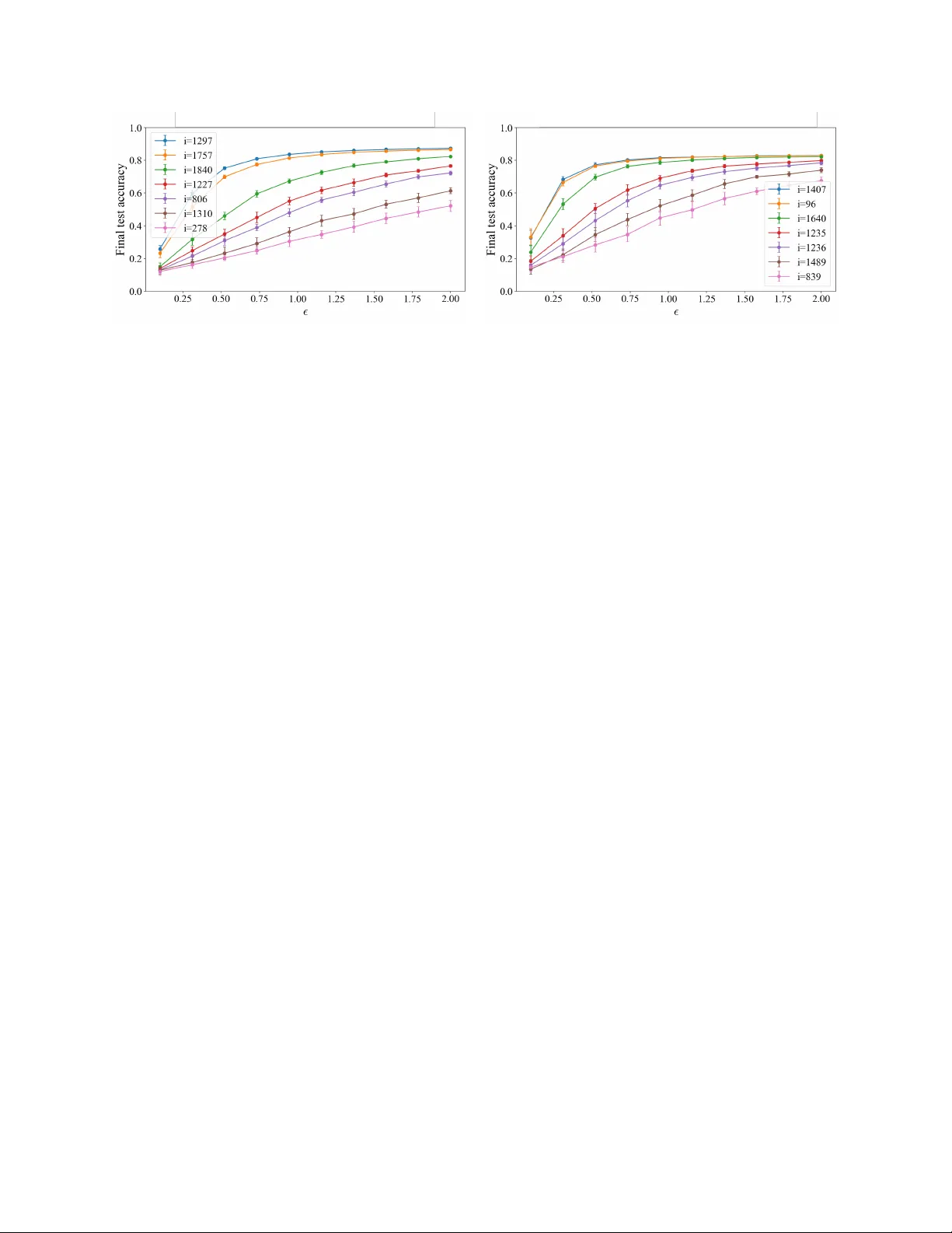
Certified P er-Instance Unlearning Using Individual Sensitivit y Bounds Hanna Benarro c h ∗ 1 , Jamal A tif 2 , and Olivier Capp é 1 1 DI ENS, École normale sup érieure, Univ ersité PSL, CNRS, 75005 Paris, F rance 2 CMAP , École p olytechnique, Institut P olytec hnique de Paris, 91120 P alaiseau, F rance Abstract Certified machine unlearning can be ac hieved via noise injection leading to differen tial priv acy guaran- tees, where noise is calibrated to worst-case sensitivity . Suc h conserv ative calibration often results in perfor- mance degradation, limiting practical applicability . In this w ork, we inv estigate an alternative approach based on adaptiv e p er-instance noise calibration tai- lored to the individual contribution of eac h data p oint to the learned solution. This raises the follo wing chal- lenge: how c an one establish formal u nle arning guar- ante es when the me chanism dep ends on the sp e cific p oint to b e r emove d? T o define individual data p oint sensitivities in noisy gradien t dynamics, we consider the use of p er-instance differen tial priv acy . F or ridge regression trained via Langevin dynamics, w e derive high-probabilit y p er-instance sensitivity bounds, yield- ing certified unlearning with substantially less noise injection. W e corrob orate our theoretical findings through exp erimen ts in linear settings and pro vide further empirical evidence on the relev ance of the approac h in deep learning settings. 1 In tro duction Mo dern mac hine learning systems increasingly op er- ate under regulatory and contractual constrain ts that require the p ost-ho c remov al of individual training ex- amples, for instance in the context of the “right to b e forgotten” ( Marino et al. , 2025 ). The gold standard is to retrain the mo del from scratc h on the dataset with the target example remov ed, but such retraining is often computationally infeasible in practice. Machine unlearning seeks to approximate the effect of retrain- ing at a substan tially low er cost, either b y enforcing exact equiv alence with retraining ( exact unle arning ) ( Cao and Y ang , 2015 ) or by matc hing the retrained ∗ Corresponding author: hanna.benarroch@ens.psl.eu mo del only in distribution ( appr oximate unle arning ) ( Ginart et al. , 2019 ; Sekhari et al. , 2021 ). W e fo cus on appr oximate unle arning . W e further restrict attention to c ertifie d unlearning, where deletion pro cedures are accompanied by explicit, pro v able guaran tees. Suc h guarantees are naturally connected to differential priv acy (DP), whic h quan- tifies how the output distribution of a randomized mec hanism changes when a single training p oint is remo ved. While DP pro vides a natural language for reasoning about certified deletion, its guarantees do not directly transfer to the unlearning setting. A first mismatc h concerns the notion of adjacency . Differen tial priv acy allows either remo ving or sub- stituting a data p oin t, whereas unlearning compares training to retraining the mo del as if a given p oint had nev er b een part of the dataset. Substitution-based adjacency therefore lacks a natural in terpretation for unlearning, although it is sometimes used for technical con venience (e.g., Chien et al. , 2024 ). The most imp ortant difference, ho wev er, lies in the nature of the guarantee itself. Differen tial priv acy cer- tifies a mechanism a priori , uniformly o ver all datasets and all data p oints. Unlearning, b y contrast, is in- heren tly p ost-ho c : it targets a sp ecific trained model, a sp ecific dataset, and a sp ecific data p oint whose deletion is requested. First, this post-ho c nature affects ho w unlearning guaran tees should b e defined. While man y existing approac hes compare unlearning to a full retraining oracle ( Ginart et al. , 2019 ; Neel et al. , 2021 ; Guo et al. , 2020 ; Kolosk o v a et al. , 2025 ; Mu and Klab jan , 2025 ), we follo w several recen t works ( Lu et al. , 2025 ; Basaran et al. , 2025 ; W aereb eke et al. , 2025 ) and adopt a self-r efer enc e d notion of unlearning, which compares t wo executions of the same unlearning pro- cedure on adjacent datasets. This isolates what is certified in trinsically by the unlearning mec hanism. Second, this conceptual difference affects how guar- an tees should b e calibrated across data p oints. Uni- 1 form DP guarantees, while stronger in generalit y , en- force an homogeneous treatment of all data p oints, regardless of their actual influence on the learned mo del. This regime is implicitly adopted by some certified unlearning approac hes, including Langevin- based methods ( Chien et al. , 2024 ). In contrast, w e argue that certified unlearning should explicitly ex- ploit the fact that deletion targets a sp ecific dataset and a sp ecific data point. This naturally calls for p er- instanc e certified unlearning, where guaran tees are calibrated to the actual influence of the p oin t b eing remo ved, a voiding unnecessary addition of noise and loss of utility . This view is supp orted b y recent w ork on individualized guarantees ( Sepahv and et al. , 2025 ) and by empirical evidence showing that worst-case sensitivit y b ounds often o verestimate the influence of t ypical data p oints ( Th udi et al. , 2024 ). W e now turn to the practical question of ho w to de- riv e certified unlearning guarantees within this frame- w ork. As in ( Chien et al. , 2024 ), we consider unlearn- ing pro cedures based on Langevin dynamics. Our anal- ysis builds on recent results b y Bok et al. ( 2024 ), who sho w how priv acy loss can b e track ed along noisy opti- mization tra jectories during learning. W e extend this reasoning to the le arn–then–unle arn setting, where the learning noise is fixed and certified deletion guar- an tees are obtained by calibrating the additional noise injected during unlearning to reach a target priv acy lev el. W e then examine ho w this analysis can b e refined at the level of individual data points. T o this end, w e introduce p er-instanc e sensitivity as the central quan tity and use it to derive certified guaran tees for appro ximate unlearning. In the case of ridge regres- sion trained with Langevin dynamics, w e show that although sensitivities are formally unbounded due to the Gaussian nature of the iterates, they can b e sharply controlled with high probabilit y and ev aluated efficien tly . This yields certified unlearning guarantees that adapt to the actual influence of the remov ed data p oin t, rather than relying on a worst-case bound. Ov erall, our results show that the difficulty of un- le arning is not uniform . Data p oin ts that exert little influence on the training dynamics are inherently eas- ier to forget and require less noise to certify their deletion, a phenomenon we analyze theoretically in the linear setting and observe empirically b eyond it. Our con tributions can b e summarized as follows: • W e adapt the shifted interpolation framew ork of Bok et al. ( 2024 ) to the learn–then–unlearn set- ting, enabling p er-instance certified unlearning. • W e deriv e sharp high-probability p er-instance sensitivit y b ounds for ridge regression un- der Langevin dynamics, yielding heterogeneous unlearning guaran tees and improv ed priv acy– accuracy trade-offs compared to uniform calibra- tion. • W e provide empirical evidence of similar instance- lev el heterogeneity in a typical deep learning set- ting, despite the lack of a supp orting theoretical analysis. 2 Related w ork Exact and appro ximate unlearning. Early work on mac hine unlearning fo cused on exact deletion, re- quiring the p ost-deletion mo del to coincide with re- training on the dataset with the remov ed p oint ( Cao and Y ang , 2015 ) (e.g., Remark 4.5 ). Such guaran- tees rely on strong structural assumptions and do not scale to mo dern learning pip elines. This motiv ated the probabilistic form ulation introduced by Ginart et al. ( 2019 ), which requires the output distribution of an unlearning algorithm to b e close to that of retraining. Our w ork adopts this probabilistic viewp oint. Gradien t-based unlearning with noisy optimiza- tion. Most unlearning metho ds inv olv e further opti- mization steps that exclude the data p oin t to b e for- gotten. Descent-to-Delete ( Neel et al. , 2021 ) p erforms additional gradien t descent steps follow ed by output p erturbation to obtain priv acy guarantees. How ev er, as sho wn by Chien et al. ( 2024 ), this approac h leads to more conserv ativ e noise calibration than injecting noise at eac h gradient step. Building on this insigh t, they proposed a Langevin-based unlearning procedure analyzed under uniform sensitivity b ounds and imple- men ting deletion via a replacement-based mechanism. Our w ork follows the same noisy-gradient paradigm but differs by considering omission-based unlearning, and b y calibrating the noise in an instance-dep enden t w ay . P er-instance unlearning mechanisms. The no- tion of p er-instanc e differ ential privacy formalizes pri- v acy guaran tees that v ary across data points ( W ang , 2019 ). Sev eral unlearning metho ds, although not refer- ing explicitly to the term p er-instanc e , deriv e instanc e- dep endent unle arning metho ds . Guo et al. ( 2020 ) use influence functions to compute Newton-style updates for general conv ex ob jectives, with priv acy guaran- tees obtained via ob jective p erturbation. Izzo et al. ( 2021 ) derive a pro jected residual up date for linear regression, remo ving the contribution of the deleted p oin t from the closed-form solution (without priv acy 2 guaran tees). While these approac hes are explicitly instance-dep enden t, they rely on parameter-level up- dates and therefore do not provide a framew ork for analyzing noisy gradient descen t. In contrast, our ap- proac h derives per-instance guarantees directly along the optimization tra jectory . Gaussian differential priv acy and priv acy ac- coun ting. Gaussian Differen tial Priv acy (GDP) ( Dong et al. , 2022 ) pro vides a hypothesis-testing-based priv acy framew ork with tigh t comp osition rules and sharp conv ersion to ( ε, δ ) guarantees. Earlier analyses of Langevin dynamics ( Chien et al. , 2024 ; Choura- sia et al. , 2021 ; Ryffel et al. , 2022 ) t ypically relied on Rényi differential priv acy , resulting in lo oser ( ε, δ ) b ounds. More recen tly , Bok et al. ( 2024 ) lev erage GDP comp osition for iterative algorithms with con- tractiv e dynamics, yielding sharp er priv acy account- ing. These analyses exploit a form of privacy ampli- fic ation by iter ation ( F eldman et al. , 2018 ), whereby the rep eated application of noisy con tractive updates yields strictly stronger guarantees than those deriv ed from w orst-case Gaussian comp osition. W e adapt this framew ork to the unlearning setting by trac king the priv acy loss along a combined learn–then–unlearn tra jectory with p er-instance sensitivity con trol. 3 Problem Setting 3.1 Regularized Empirical Risk Mini- mization W e consider sup ervised learning with a dataset D = { ( x j , y j ) } n j =1 , where x j ∈ R p and y j ∈ R d . Given a p er-example loss ℓ ( θ ; x, y ) and a regularizer r ( θ ) , w e define the non-aver age d regularized empirical risk minimization (ERM) ob jective f D ( θ ) := n X j =1 ℓ ( θ ; x j , y j ) + λ r ( θ ) , (1) where λ > 0 . F or a designated index i ∈ { 1 , . . . , n } corresp onding to a deletion request, we define the le ave-one-out ob jective f D − i ( θ ) := X j  = i ℓ ( θ ; x j , y j ) + λ r ( θ ) , (2) whic h corresp onds to training on the retain set with the p oin t ( x i , y i ) remov ed. Throughout the paper, un- learning is understo o d as transforming a mo del trained (appro ximately) with resp ect to f D in to one whose distribution is close to that obtained by optimizing f D − i . 3.2 Certified p er-instance unlearning W e briefly recall the standard notion of differential priv acy . Definition 3.1 (Differen tial Priv acy ( Dwork et al. , 2006 )) . A randomized algorithm A is ( ε, δ ) - differen tially priv ate if for any pair of adjacent (e.g. differing from one data point) datasets D , D ′ and an y measurable set S , P ( A ( D ) ∈ S ) ≤ e ε P ( A ( D ′ ) ∈ S ) + δ. Differen tial priv acy provides a distributional indis- tinguishabilit y guarantee with resp ect to the presence or absence of a single data p oint in the input dataset. Unlearning aims at removing the influence of a desig- nated for get set or for get p oint from a trained mo del. In certified mac hine unlearning, this is formalized by requiring that the output of the unlearning pro cedure b e statistically indistinguishable from an output that do es not depend on the forgotten data. The dominan t formalization in the early literature w as introduced by Ginart et al. ( 2019 ). Definition 3.2 ( ( ε, δ ) -Reference Unlearning ( Ginart et al. , 2019 )) . An unlearning algorithm U satisfies ( ε, δ ) -reference unlearning if there exists a r efer enc e algorithm A suc h that, for any retain dataset D r , forget dataset D f , and any measurable set S , P ( U ( A ( D ) , D r , D f ) ∈ S ) ≤ e ε P ( A ( D r ) ∈ S ) + δ, W aereb ek e et al. , 2025 refer to this definition as r efer enc e unle arning , as the guarantee is stated relativ e to an external reference algorithm A , typically taken to b e retraining from scratch on the retain set D r . As emphasized in subsequent works (e.g., Georgiev et al. , 2024 , W aereb eke et al. , 2025 ), this definition is unsatisfactory b oth conceptually and practically , since it dep ends on the reference algorithm rather than on the unlearning pro cedure alone. T o av oid this dep endence, Sekhari et al. ( 2021 ) pro- p osed a stronger definition that instead compares U to itself on adjacent unlearning scenarios. Concretely , ( ε, δ ) -unlearning implies ( ε, δ ) -reference unlearning by taking A ′ ( D r ) = U ( A ( D r ) , D r , ∅ ) , whereas the con- v erse need not hold in general. Definition 3.3 ( ( ε, δ ) -Unlearning ( Sekhari et al. , 2021 )) . An unlearning algorithm U satisfies ( ε, δ ) - unlearning if for a given learning algorithm A and an y retain dataset D r , forget dataset D f , and any measurable set S , P ( U ( A ( D ) , D r , D f ) ∈ S ) ≤ e ε P ( U ( A ( D r ) , D r , ∅ ) ∈ S ) + δ. 3 The ab o ve definition do es not dep end on the forget set or data p oint. W e sp ecifically fo cus on the relev ant setting where the deletion request targets a sp e cific data p oint and introduce p er-instanc e unle arning (see Figure 1 for intuition). Definition 3.4 ( ( ε, δ ) -P er-Instance Unlearning) . Let A b e a randomized learning algorithm and U an un- learning algorithm. F or a dataset D and a point ( x i , y i ) ∈ D , the algorithm U satisfies ( ε, δ ) -p er- instance unlearning if for any measurable set S , P  U ( A ( D ) , D − i , ( x i , y i )) ∈ S  ≤ e ε P  U ( A ( D − i ) , D − i , ∅ ) ∈ S  + δ where D − i := D \ { ( x i , y i ) } . Before unlearning A ( D ) A ( D − i ) O ( ε 0 ) After unlearning U ( A ( D ) , D − i , ( x i , y i )) U ( A ( D − i ) , D − i , ∅ ) O ( ε ) Figure 1: Intuition b ehind p er-instance unlearning. T op: After training, the parameter distributions in- duced by A ( D ) and A ( D − i ) are sharply concen trated and well separated, resulting in a large priv acy gap ε 0 . Bottom: After applying the unlearning pro- cedure U , the resulting distributions corresp onding to U ( A ( D ) , D − i , ( x i , y i )) and U ( A ( D − i ) , D − i , ∅ ) b e- come closer, yielding a m uch smaller priv acy parame- ter ε ≪ ε 0 . Unlik e standard differential priv acy , p er-instance unlearning tailors its guaran tees to the specific data p oin t ( x i , y i ) targeted b y the deletion request. The analysis therefore aims to quantify the amount of noise and computation required so that the p ost-ho c un- learned output matches, in distribution, the outcome that would ha ve b een obtained had the p oint nev er b een included in the training set. 3.3 Algorithms: learn then targeted unlearn W e in tro duce our learning algorithm A and unlearning algorithm U . Langevin learning A Giv en a step size η and an initial noise level σ learn , the discrete Langevin up date is θ k +1 = θ k − η ∇ θ f D ( θ k ) + q 2 η σ 2 learn ξ k , ξ k ∼ N (0 , I ) . (3) After T steps, θ T ∼ A ( D ) . W e require σ learn > 0 (p ossibly v ery small) so that the learning algorithm A is randomized and induces a non-degenerate output distribution. This random- ness is necessary to quantify the priv acy loss b etw een training on D and retraining on the retain dataset D − i . T argeted unlearning U via retain-set fine- tuning Giv en an unlearning request for ( x i , y i ) , we run K additional Langevin steps on D − i with cali- brated noise level σ unlearn : θ k +1 = θ k − η ∇ θ f D − i ( θ k ) + q 2 η σ 2 unlearn ξ k , ξ k ∼ N (0 , I ) . (4) The output is θ T + K ∼ U ( A ( D ) , D − i , ( x i , y i )) . 4 Theory for Certified P er- instance Unlearning W e trac k the priv acy loss along the optimization tra- jectory generated b y the learning and unlearning al- gorithms A and U (Prop osition 4.2 ). This analysis explicitly reveals how priv acy guarantees dep end on in- dividual data p oin ts, as captured by their p er-instanc e sensitivities. Our k ey contribution is Theorem 4.3 , whic h leverages a high-probabilit y con trol of these sensitivities to derive ( ε, δ ) -p er-instance unlearning guaran tees (in the sense of Definition 3.4 ) for ridge regression. 4.1 Priv acy loss trac king under con- tractiv e up dates and p er-instance sensitivit y W e rely on the shifted in terp olation framework of Bok et al. ( 2024 ) to track priv acy loss along the optimiza- tion tra jectory . This analysis crucially relies on the con traction of the deterministic gradient map asso ci- ated with Langevin dynamics, which yields priv acy amplification by iteration ( F eldman et al. , 2018 ). W e formalize this requirement in the follo wing assump- tion. 4 Assumption 4.1. Both ob jectives f D and f D − i are differen tiable, m -strongly conv ex and L -smo oth. Un- der these assumptions, the gradient map Φ( θ ) = θ − η ∇ f ( θ ) is contractiv e for any step size 0 < η < 2 /L , with contraction factor c = max { | 1 − η m | , | 1 − η L | } ( Bub ec k , 2015 ; Nesterov , 2004 ). T o ensure a strict con traction ( c < 1 ), we fix η = 1 /L , yielding c = 1 − η m < 1 . F ollowing ( Bok et al. , 2024 ), we work within the Gaussian Differential Priv acy (GDP) framework. F or µ -GDP guarantees, w e denote b y ε GDP ( µ, δ ) the v alue of ε suc h that ( ε, δ ) -differen tial priv acy holds. F ormal definitions of GDP and the con version from µ to ( ε, δ ) are giv en in App endix A . Compared tra jectories for priv acy analysis. The analyzed priv acy gap is measured b et ween tw o pa- rameter tra jectories ( θ k ) k ≥ 0 and ( θ ′ k ) k ≥ 0 (see Figure 2 ) initialized at the same deterministic p oin t θ 0 = θ ′ 0 . The (real) tra jectory ( θ k ) follo ws learning algorithm A on the full dataset D for T iterations with noise lev el σ learn > 0 , and K unlearning steps via U on the retain set D − i with noise lev el σ unlearn > 0 . The second tra jectory ( θ ′ k ) corresp onds to the (theoreti- cal) retraining path, obtained b y running the same learning and unlearning pro cedures directly on D − i . k 0 T T + K θ 0 = θ ′ 0 θ T θ T + K θ ′ T θ ′ T + K ∆ i,k > 0 ∆ i,k = 0 Figure 2: Learn–unlearn vs. retraining tra jectories. The solid path ( θ k ) corresp onds to training on the full dataset D follo wed b y unlearning, while the dashed path ( θ ′ k ) corresp onds to (fictitious ly) training and retraining on the retain dataset D − i . Prop osition 4.2 (Gaussian DP accounting of the unlearning mec hanism U for bounded p er-instance sensitivities) . Consider the two p ar ameter tr aje ctories ( θ k ) k ≥ 0 and ( θ ′ k ) k ≥ 0 define d as ab ove. Assume that Assumption 4.1 holds with c ontr action factor c < 1 . F or an unle arning r e quest c onc erning ( x i , y i ) , define the p er-instanc e sensitivity at time k as ∆ i,k = ∥ η  ∇ f D − i ( θ k ) −∇ f D ( θ k )  ∥ = η ∥∇ ℓ ( θ k ; x i , y i ) ∥ and assume that ther e exists a deterministic se quenc e { s i,k } T k =0 (which do es not dep end on the sto chastic tr aje ctory of θ k ) such that ∀ k ≤ T , ∆ i,k ≤ s i,k . Then, the final outputs θ T + K and θ ′ T + K satisfy µ - Gaussian Differ ential Privacy with p ar ameter µ i T + K given by, µ i T + K = P T k =0 c T + K − k s i,k √ V learn + V unlearn , with V learn := T X k =0 2 η σ 2 learn c 2( T + K − k ) , V unlearn := T + K X k = T +1 2 η σ 2 unlearn c 2( T + K − k ) . In p articular, for any δ ∈ (0 , 1) , the unle arn- ing me chanism U achieves ( ε GDP ( µ i T + K , δ ) , δ ) -p er- instanc e unle arning (in the sense of Definition 3.4 ). 4.2 Limits of deterministic sensitivit y b ounds Prop osition 4.2 relies on deterministic b ounds on the p er-step sensitivities ∆ i,k . In general, suc h bounds re- quire either the loss gradien t to b e uniformly b ounded, or the loss to b e Lipschitz in θ . These assumptions exclude imp ortan t settings, including standard linear regression. Moreov er, when Gaussian noise is used, the iterates θ k ha ve un b ounded supp ort; if the loss gradien t is unbounded, this directly implies that ∆ i,k itself cannot b e deterministically b ounded. This situation arises naturally in ridge regression trained by Langevin dynamics. In this case, sensitivi- ties are neither uniformly b ounded nor deterministic, and their distribution has unbounded supp ort due to the Gaussian nature of the iterates. How ev er, our key con tribution in Theorem 4.3 is to exploit the Gaus- sian structure of the point wise gradient loss in ridge regression to derive sharp high-pr ob ability sensitivit y b ounds and calibrate unlearning noise to the data p oin t to unlearn. 4.3 Certified p er-instance unlearning guaran tees in the case of Ridge regression In this section, we consider multi-output linear ridge regression with inputs X ∈ R n × p , outputs Y ∈ R n × d , and parameter θ ∈ R p × d with deterministic initializa- tion θ 0 . The ob jective is f D ( θ ) = n X j =1 1 2 ∥ x ⊤ j θ − y j ∥ 2 2 + λ 2 ∥ θ ∥ 2 F , 5 Theorem 4.3 (Certified p er-instance unlearning for ridge regression) . Consider the multi-output line ar ridge r e gr ession setting intr o duc e d ab ove, tr aine d with le arning algorithm A and noise σ learn > 0 for T it- er ations. Assume that Assumption 4.1 holds with c ontr action factor c < 1 . Supp ose we want to unle arn a data p oint ( x i , y i ) in the sense of Definition 3.4 with fixe d tar get privacy level ( ε, δ ) ∈ (0 , ∞ ) × (0 , 1) , and a fixe d unle arning horizon K ≥ 1 . (i) High-probability p er-instance sensitivities. Set δ s ∈ (0 , δ ) . Ther e exists an explicit, data- dep endent se quenc e { s δ s i,k } T k =0 such that P  ∀ k ≤ T , ∆ i,k = η ∥∇ ℓ ( θ k ; x i , y i ) ∥ F ≤ s δ s i,k  ≥ 1 − δ s , wher e e ach s δ s i,k is c omputable in close d form fr om ( X, Y , x i , y i , σ learn , T ) via a nonc entr al χ 2 quantile (se e Pr op osition 4.4 ). (ii) Calibration of unlearning noise. Set δ m = δ − δ s . Then the minimal unle arning noise level which satisfies ( ε, δ ) -p er-instanc e unle arning of ( x i , y i ) in the sense of Definition 3.4 is define d as σ unlearn := arg min σ ≥ 0 n σ : ε GDP  µ i ( σ ) , δ m  ≤ ε o , wher e µ i ( σ ) := P T k =0 c T + K − k s δ s i,k p V learn + V unlearn ( σ ) . V learn and V unlearn ar e define d in Pr op osition 4.2 . Prop osition 4.4 (High-probability sensitivit y b ounds s δ s i,k for ridge regression) . Consider the multi-output line ar ridge r e gr ession setting intr o duc e d ab ove. Define the data-dep endent matric es M := I p − η ( X ⊤ X + λI p ) , B := X ⊤ Y . F or a fixe d data p oint ( x i , y i ) and e ach iter ation k ≥ 0 , the r esidual r i,k := x ⊤ i θ k − y i ∼ N ( µ i,k , v i,k I d ) , wher e µ i,k := x ⊤ i  M k θ 0 + η k − 1 X j =0 M j B  − y i , v i,k := 2 η σ 2 learn k − 1 X j =0 ∥ ( M j ) ⊤ x i ∥ 2 2 . It fol lows that ∥ r i,k ∥ 2 2 v i,k ∼ χ ′ 2 d  ∥ µ i,k ∥ 2 2 v i,k  , that is, a non-c entr al chi-squar e distribution with d de gr e es of fr e e dom and non-c entr ality p ar ameter ∥ µ i,k ∥ 2 2 /v i,k . As ∆ i,k = η ∥ x i ∥ 2 ∥ r i,k ∥ 2 , for any δ s ∈ (0 , 1) define s δ s i,k := η ∥ x i ∥ 2 q v i,k q i,k  1 − δ s T  , wher e q i,k ( · ) denotes the quantile function of the ab ove χ ′ 2 d distribution. Then, P  ∀ k ≤ T , ∆ i,k ≤ s δ s i,k  ≥ 1 − δ s . R emark 4.5 (Exact unlearning for ridge regression) . F or ridge regression, exact unlearning is p ossible when targeting the exact regularized least-squares (LS) so- lution. In particular, letting A := X ⊤ X + λI p and H := X A − 1 X ⊤ , the lea ve-one-out (LOO) prediction admits the closed form ˆ y ( − i ) i = ˆ y i − ˆ y i − y i 1 − ( H ) ii , where ˆ y = H y , whic h follo ws from the Sherman–Morrison form ula ( Golub et al. , 1979 ; Hastie et al. , 2004 ). Ho wev er, this closed-form expression applies only at the exact LS solution. Using this form ula prior to conv ergence introduces a discrepancy with exact unlearning and, moreo ver, cannot b e safeguarded by a standard DP mec hanism to ensure v alid priv acy guar- an tees. As a result, the LOO form ula do es not solve the unlearning problem in the finite-time regime that w e consider and offers limited p oten tial for general- ization beyond the linear case. F rom a computational standp oin t, applying the LOO form ula also requires forming the hat matrix and explicitly inv erting the normal matrix A , whose cost and numerical stabil- it y degrade rapidly with the dimension p , especially in weakly regularized regimes. While our approach also in volv es storing the hat matrix, it a v oids any ma- trix in version and operates directly through iterativ e up dates. 5 Exp erimen ts 5.1 Linear setting In this section, w e implement Algorithm 1 (see Ap- p endix D.1 ), which describ es the complete learning and unlearning pip eline. T ask and setup. W e consider image classification on MNIST ( Lecun et al. , 1998 ) with a fixed-feature pip eline: images are mapp ed to represen tations ϕ ( x ) b y a frozen ResNet-50 bac kb one, and only a m ulti- output ridge regression head ( d = 10 ) is trained. Pre- dictions are obtained b y taking the arg max o ver the 6 Figure 3: High-probability sensitivit y b ounds s δ s i,k for all MNIST training points in the linear ridge regres- sion setting. Ro ws corresp ond to data p oints and columns to learning iterations. Poin ts are sorted by increasing final sensitivity s δ s i,T , highligh ting substan- tial p er-instance heterogeneity already at the level of analytical b ounds. head outputs. All unlearning op erations therefore tak e place in a linear, strongly conv ex regime. T raining and unlearning. Learning is performed for T = 300 gradient steps on the full dataset D , follo wed b y K = 30 additional steps on the reduced dataset D − i to unlearn a single p oint (see the ab- lation study on K in App endix D.2 ). W e use ℓ 2 - regularization with λ = 10 − 4 and set the step size to η = 1 /L , so that the gradient map is contractiv e with factor c = 1 − m/L (Assumption 4.1 ). Gaussian noise with standard deviation σ learn = 0 . 01 is injected during learning, while the unlearning noise σ unlearn is calibrated to reac h a target ( ε, δ ) guaran tee, and we con ven tionally take δ = 1 /n . P er-instance sensitivity along training. Propo- sition 4.4 provides, for each training p oint, a deter- ministic high-probabilit y b ound { s δ s i,k } k ≤ T on its p er- step sensitivit y . Figure 3 visualizes these b ounds for all MNIST training p oin ts and reveals pronounced heterogeneit y across b oth p oints and iterations, in- dicating that a single uniform sensitivity b ound is inheren tly misleading. W e additionally v erify that the analytical b ounds are not o verly conserv ative by comparing them to empirical sensitivities measured along Langevin training tra jectories; see Figure 7 in App endix. Selection of p oints to unlearn. In practice, exhaustiv ely unlearning ev ery data point is computa- tionally prohibitiv e. Motiv ated b y the heterogeneity rev ealed in Figure 3 , we therefore fo cus on a small set of represen tative points spanning differen t sensi- tivit y regimes. W e select 7 indices based on their difficulty at con vergence, measured by the norm of the p er-sample gradien t ∥∇ θ ℓ ( θ T ; x i , y i ) ∥ after one full (random) training on D . Poin ts are ranked according to this quan tity and we retain the easiest p oin t, the hardest p oint, and sev eral in termediate quan tiles (see Figure 4 ). Figure 4: Representativ e MNIST examples selected for unlearning, ordered from left to right by increasing difficult y , as measured by the p er-sample gradient norm ∥∇ θ ℓ ( θ T ; x i , y i ) ∥ at conv ergence for a certain seed. Priv acy–utility trade-off. Figure 5 shows the priv acy–utilit y trade-off induced by unlearning. All curv es report test accuracy av eraged ov er 20 indep en- den t runs of the learning–unlearning pro cedure. As exp ected, stronger priv acy guaran tees (smaller ε ) re- quire injecting more noise and lead to low er accuracy . Solid lines corresp ond to p er-instanc e unlearning (our metho d), while dashed lines denote a uniform baseline that follo ws the same contractiv e optimiza- tion dynamics and Gaussian DP accoun ting but relies on a single global sensitivit y b ound shared across all p oin ts (see App endix D.2 ). This uniform calibration assumes oracle kno wledge of the maximal gradient magnitude encountered during training and applies the same worst-case noise level to all deletion requests. As illustrated in Figure 5 , p er-instance calibration rev eals a pronounced heterogeneit y in the priv acy– utilit y trade-off. A t a fixed priv acy budget ε , p ost- unlearning accuracy v aries substan tially across re- mo ved p oin ts, highlighting that the difficulty of un- learning is inheren tly p oint-dependent. The uniform baseline fails to adapt to this v ariabilit y , resulting in o verly conserv ative beh a vior for most data points. In con trast, per-instance calibration consistently achiev es a more fav orable priv acy–utility trade-off. App endix D.2 reports the p er-instance unlearning noise lev els σ unlearn , whic h v ary b y up to a factor of fiv e across data p oints for a fixed priv acy target. 5.2 Non-linear setting W e no w turn to a non-linear setting in order to assess whether the heterogeneity observ ed in the linear case p ersists for realistic deep learning mo dels. Mo del and data. W e consider image classifica- tion on CIF AR-10 ( Krizhevsky and Hinton , 2009 ). The predictor is a conv olutional neural netw ork with a VGG-st yle arc hitecture, trained end-to-end with 7 Figure 5: Priv acy–utilit y trade-off on MNIST. Final test accuracy as a function of the priv acy budget ε for p er-instance unlearning (solid lines) and a uniform baseline (dashed lines). Eac h curve corresp onds to a distinct remov ed training p oint, highligh ting the heterogeneit y of the trade-off across p oints. gradien t descent. The optimization problem is non- con vex and the training dynamics dep end strongly on the tra jectory . T raining and unlearning. W e train for T = 500 steps on the dataset D with learning rate η = 10 − 2 , full batch (to av oid in tro ducing extra randomness from mini-batc h sampling), using ℓ 2 -regularization with λ = 10 − 4 and full gradien t clipping at C = 1 . 0 (as it is a common practice when training neural net works under priv acy constrain ts). Unlearning contin ues for K = 20 steps on D − i . During learning we inject no noise ( σ learn = 0 . 0 ), and, crucially , the same Gaussian noise level σ unlearn = 0 . 02 is used for all p oin ts during unlearning (no p er-point calibration). Although this pro cedure constitutes a very natural extension of our previous unlearning algorithm to this non-linear set- ting, it is impossible to certify that Definition 3.4 is satisfied with any level of priv acy guaran tee. W e will th us use b elow an emprical auditing metho d to asses the individual priv acy guaran tees after unlearning. Represen tative p oin ts. T o prob e heterogeneity without exhaustively unlearning all samples, we se- lect a small set of represen tative indices based on an early-training proxy . After 50 noiseless train- ing steps, w e compute the p oin twise gradien t norms ∥∇ θ ℓ ( θ 50 ; x i , y i ) ∥ and select indices at fixed quan tiles of this distribution, spanning w eakly to strongly influ- en tial p oints (see Figure 6 ). All subsequen t unlearning exp erimen ts are p erformed on these fixed indices. Mon te Carlo protocol. T o account for the sto c hasticity induced b y the random initialization and the injected Gaussian unlearning noise, the en tire unlearning pro cedure is rep eated R = 50 times for eac h index i . All rep orted quantities are computed Figure 6: Representativ e CIF AR-10 samples selected at fixed quantiles of the early-training p oint wise gra- dien t norm. These images corresp ond to the indices used in T able 1 . from the aggregated distributions obtained o ver these R runs. Empirical priv acy ev aluation. F or each index i , w e compare the distribution of final mo del parameters obtained b y unlearning ( x i , y i ) with the distribution obtained by retraining from scratch on D − i with the same proto col ( T steps with no noise σ learn = 0 . 0 and K steps with σ unlearn = 0 . 02 ). W e estimate the corresp onding h yp othesis-testing trade-off curve β i ( α ) using a linear distinguisher on the mo del logits ev aluated on a fixed probe set. F rom the resulting empirical trade-off curv e, we fit a Gaussian differential priv acy (GDP) parameter µ i defined b y β i ( α ) ≈ Φ  Φ − 1 (1 − α ) − µ i  . W e observe that this Gaussian approximation provides a go od fit to the empirical trade-off curv es across all represen tative points, supp orting the use of GDP as a meaningful empirical summary even in non-con vex settings (see App endix D.3 for quantitativ e fit diagnos- tics). F or interpretabilit y , we con vert each µ i in to an ( ε i , δ ) guarantee by fixing δ = 1 /n , and numerically in verting the standard GDP-to-DP con version. T able 1: Non-linear unlearning on CIF AR-10. Re- p orted v alues are obtained b y aggregating R = 50 indep enden t runs p er p oint. All p oints are unlearned using the same noise level σ unlearn , y et the resulting priv acy guaran tees ε i (computed at δ = 1 /n ) exhibit substan tial heterogeneity . Index i AUC ˆ µ i ˆ ε i ( δ = 1 /n ) 358 0.670 0.754 2.05 471 0.764 1.062 3.14 418 0.743 1.017 2.98 381 0.747 1.095 3.26 483 0.822 1.614 5.38 90 0.821 1.384 4.41 226 0.950 2.313 8.69 Key observ ations. Despite using the same un- learning noise for all p oin ts, the resulting effe ctive priv acy guarantees v ary substantially across indices. 8 As sho wn in T able 1 , the fitted GDP parameters ˆ µ i differ significantly across represen tative points, whic h translates into a wide range of effective priv acy lev els ˆ ε i (at δ = 1 /n ). These results highlight a fundamental limitation of uniform unlearning noise in non-linear mo dels: when the same noise level is applied to all p oin ts—an approach that implicitly assumes uniform influence—the resulting priv acy guaran tees v ary sub- stan tially and dep end on how strongly each data point affects the training tra jectory . 6 Conclusion In this work, w e prop ose a p oin t-dep endent view of certified mac hine unlearning, which allows the noise calibration to dep end on the specific data p oin t b eing remo ved. W e find this p ersp ectiv e particularly rele- v an t, as it leads to a credible unlearning pro cedure in the ridge regression mo del, in con trast to uniform w orst-case calibration that results in a severe loss of accuracy after unlearning. Our theoretical guarantees rely on training dynam- ics exhibiting a form of contraction, which is essential for the tra jectory-level GDP accoun ting. This as- sumption is satisfied for strongly conv ex and smo oth ob jectives, suc h as ridge regression, but generally do es not hold for end-to-end deep netw orks, ev en when us- ing gradient clipping. This b eing said, the linear case already corresp onds to a concrete and practically rele- v an t use case, since linear mo dels naturally arise when only the final prediction head of a neural netw ork is trained, while the feature extractor is kept fixed. Despite this theoretical limitation, our exp eriments on non-linear models reveal large v ariations in effec- tiv e priv acy levels across data p oints under identical unlearning noise. In particular, the v ariability in ˆ ε i v alues is of the same order of magnitude as the v ari- abilit y observed in p er-instance unlearning noise for ridge regression. This suggests that heterogeneous un- learning difficulty is not confined to the conv ex linear setting and motiv ates the developmen t of principled p er-instance guaran tees for more general training dy- namics. Broader Impact This work contributes to the study of mac hine un- learning, with the goal of enabling reliable post-ho c data deletion without full retraining. Such capabil- ities are relev ant for priv acy regulation compliance, data gov ernance, and user control o ver personal data in deplo yed machine learning systems. Overall, we exp ect this work to support the developmen t of more accoun table and interpretable unlearning mechanisms, rather than enabling new forms of misuse. References Umit Yigit Basaran, Sk Mira j Ahmed, Amit Ro y- Cho wdhury , and Basak Guler. A certified unlearn- ing approach without access to source data. In F orty-se c ond International Confer enc e on Machine L e arning , 2025. Jinho Bok, W eijie J. Su, and Jason Altsch uler. Shifted in terp olation for differen tial priv acy . In Pr o c e e dings of the 41st International Confer enc e on Machine L e arning , ICML’24. JMLR.org, 2024. Sébastien Bub ec k. Conv ex optimization: Algorithms and complexity . F ound. T r ends Mach. L e arn. , 8 (3–4):231–357, 2015. Yinzhi Cao and Junfeng Y ang. T ow ards making sys- tems forget with machine unlearning. In 2015 IEEE Symp osium on Se curity and Privacy , pages 463–480, 2015. Eli Chien, Hao yu Peter W ang, Ziang Chen, and Pan Li. Langevin unlearning: A new p erspective of noisy gradien t descent for machine unlearning. In The Thirty-eighth A nnual Confer enc e on Neur al Information Pr o c essing Systems , 2024. Risha v Chourasia, Jiayuan Y e, and Reza Shokri. Dif- feren tial priv acy dynamics of langevin diffusion and noisy gradient descent. In M. Ranzato, A. Beygelz- imer, Y. Dauphin, P .S. Liang, and J. W ortman V aughan, editors, A dvanc es in Neur al Information Pr o c essing Systems , v olume 34, pages 14771–14781. Curran Asso ciates, Inc., 2021. Jinsh uo Dong, Aaron Roth, and W eijie J. Su. Gaussian differen tial priv acy . Journal of the R oyal Statistic al So ciety Series B: Statistic al Metho dolo gy , 84(1):3– 37, 02 2022. Cyn thia Dwork, F rank McSherry , K obbi Nissim, and A dam Smith. Calibrating noise to sensitivity in priv ate data analysis. In The ory of Crypto gr aphy Confer enc e (TCC) , pages 265–284. Springer, 2006. Vitaly F eldman, Ilya Mironov, Kunal T alwar, and Abhradeep Thakurta. Priv acy amplification by it- eration. In 2018 IEEE 59th Annual Symp osium on F oundations of Computer Scienc e (FOCS) , page 521–532. IEEE, Octob er 2018. 9 Kristian Georgiev, Roy Rinberg, Sung Min Park, Shiv am Garg, Andrew Ily as, Aleksander Madry , and Seth Neel. A ttribute-to-delete: Machine unlearning via datamo del matc hing. CoRR , abs/2410.23232, 2024. An tonio Ginart, Melo dy Y. Guan, Gregory V aliant, and James Zou. Making AI forget you: Data dele- tion in machine learning. In A dvanc es in Neur al Information Pr o c essing Systems (NeurIPS) , 2019. Gene H. Golub, Mic hael Heath, and Grace W ahba. Generalized cross-v alidation as a metho d for c ho os- ing a go od ridge parameter. T e chnometrics , 21(2): 215–223, 1979. Ch uan Guo, T om Goldstein, A wni Hannun, and Lau- rens V an Der Maaten. Certified data remo v al from mac hine learning mo dels. In Pr o c e e dings of the 37th International Confer enc e on Machine L e arn- ing (ICML) , volume 119 of Pr o c e e dings of Machine L e arning R ese ar ch , pages 3832–3842. PMLR, 2020. T rev or Hastie, Rob ert Tibshirani, Jerome F riedman, and James F ranklin. The elemen ts of statistical learning: Data mining, inference, and prediction. Math. Intel l. , 27:83–85, 11 2004. Zac hary Izzo, Mary Anne Smart, Kamalik a Chaud- h uri, and James Zou. Approximate data deletion from machine learning mo dels. In Pr o c e e dings of The 24th International Confer enc e on Artificial In- tel ligenc e and Statistics (AIST A TS) , v olume 130 of Pr o c e e dings of Machine L e arning R ese ar ch , pages 2008–2016. PMLR, 2021. Anastasia Kolosk o v a, Y oussef Allouah, Animesh Jha, Rac hid Guerraoui, and Sanmi Ko y ejo. Certified unlearning for neural netw orks. In F orty-se c ond In- ternational Confer enc e on Machine L e arning , 2025. Alex Krizhevsky and Geoffrey Hinton. Learning mul- tiple lay ers of features from tiny images. T echnical Rep ort 0, Univ ersity of T oronto, T oronto, On tario, 2009. Y ann Lecun, Y ere Y ere, Patric k Haffner, Y o eso ep Rac hmad, and Leon Bottou. Gradient-based learn- ing applied to do cumen t recognition. Pr o c e e dings of the IEEE , 86:2278 – 2324, 12 1998. Linda Lu, A yush Sekhari, and Karthik Sridharan. System-a ware unlearning algorithms: Use lesser, forget faster. In Aarti Singh, Maryam F azel, Daniel Hsu, Simon Lacoste-Julien, F elix Berkenk amp, T egan Mahara j, Kiri W agstaff, and Jerry Zhu, edi- tors, Pr o c e e dings of the 42nd International Confer- enc e on Machine L e arning , v olume 267 of Pr o c e e d- ings of Machine L e arning R ese ar ch , pages 40560– 40592. PMLR, 13–19 Jul 2025. Bill Marino, Meghdad Kurmanji, and Nicholas D. Lane. Position: Bridge the gaps b etw een mac hine unlearning and AI regulation. In The Thirty-Ninth A nnual Confer enc e on Neur al Information Pr o c ess- ing Systems Position Pap er T r ack , 2025. Siqiao Mu and Diego Klab jan. Rewind-to-delete: Cer- tified mac hine unlearning for nonconv ex functions. In The Thirty-ninth A nnual Confer enc e on Neur al Information Pr o c essing Systems , 2025. Seth Neel, Aaron Roth, and Saeed Sharifi-Malv a jerdi. Descen t-to-delete: Gradient-based methods for ma- c hine unlearning. In Vitaly F eldman, Katrina Ligett, and Siv an Sabato, editors, Pr o c e e dings of the 32nd International Confer enc e on A lgorithmic L e arn- ing The ory , volume 132 of Pr o c e e dings of Machine L e arning R ese ar ch , pages 931–962. PMLR, 16–19 Mar 2021. Y urii Nesterov. Intr o ductory L e ctur es on Convex Optimization , v olume 87 of Applie d Optimization . Springer, New Y ork, NY, 2004. Théo Ryffel, F rancis Bach, and Da vid Poin tc hev al. Dif- feren tial Priv acy Guaran tees for Sto chastic Gradi- en t Langevin Dynamics. w orking pap er or preprint, F ebruary 2022. A yush Sekhari, Jay adev A chary a, Gautam Kamath, and Ananda Theertha Suresh. Remember what you w ant to forget: Algorithms for machine unlearn- ing. In A dvanc es in Neur al Information Pr o c essing Systems (NeurIPS) , 2021. Nazanin Mohammadi Sepah v and, Anvith Thudi, Beriv an Isik, Ashmita Bhattacharyy a, Nicolas P a- p ernot, Eleni T riantafillou, Daniel M. Ro y , and Gin tare Karolina Dziugaite. Leveraging p er- instance priv acy for mac hine unlearning. In F orty- se c ond International Confer enc e on Machine L e arn- ing , 2025. An vith Thudi, Hengrui Jia, Casey Meehan, Ilia Shu- mailo v, and Nicolas Papernot. Gradien ts look alik e: Sensitivit y is often ov erestimated in DP-SGD. In 33r d USENIX Se curity Symp osium (USENIX Se cu- rity 24) , pages 973–990, Philadelphia, P A, August 2024. USENIX Asso ciation. 10 Martin V an W aerebeke, Marco Lorenzi, Gio v anni Neglia, and Kevin Scaman. When to forget? com- plexit y trade-offs in machine unlearning. In F orty- se c ond International Confer enc e on Machine L e arn- ing , 2025. Y u-Xiang W ang. Per-instance differen tial priv acy . Journal of Privacy and Confidentiality , 9(1), Mar. 2019. 11 A Gaussian Differen tial Priv acy W e recall the definition of Gaussian Differen tial Priv acy (GDP) in tro duced by Dong et al. ( 2022 ), together with its conv ersion to ( ε, δ ) -differen tial priv acy . Definition A.1 (Gaussian Differential Priv acy ( Dong et al. , 2022 )) . F or tw o distributions P and Q , define the tr ade-off function T ( P , Q ) : [0 , 1] → [0 , 1] b y T ( P , Q )( α ) := inf ϕ : P P ( ϕ =1) ≤ α P Q ( ϕ = 0) , where the infimum ranges o ver all (p ossibly randomized) tests ϕ . An algorithm A satisfies µ -Gaussian Differen tial Priv acy ( µ -GDP) if, for any adjacent datasets D , D ′ , T  La w ( A ( D )) , Law ( A ( D ′ ))  ≥ G ( µ ) , where G ( µ ) is the trade-off function b et ween N (0 , 1) and N ( µ, 1) . A µ -GDP guaran tee implies ( ε, δ ) -differen tial priv acy for any ε > 0 , with δ = Φ  − ε µ + µ 2  − e ε Φ  − ε µ − µ 2  , (5) where Φ denotes the standard normal cumulativ e distribution function. Accordingly , for any δ ∈ (0 , 1) , one can obtain an exact conv ersion from µ -GDP to ( ε, δ ) -DP b y defining ε GDP ( µ, δ ) as the unique v alue of ε that satisfies ( 5 ). B Pro of of P rop osition 4.2 W e adapt the shifted interpolation framework of Bok et al. ( 2024 ) to the learn–unlearn setting. Setup. Let D and D − i b e neigh b oring datasets differing by a single point i . W e consider tw o tra jectories initialized at the same p oin t θ 0 = θ ′ 0 and ev olving as θ k +1 = ϕ ( θ k ) + Z k +1 , θ ′ k +1 = ϕ ′ ( θ ′ k ) + Z ′ k +1 , k = 0 , . . . , T + K, where the deterministic up date maps are ϕ ( θ ) = ( θ − η ∇ θ f D ( θ ) , k ≤ T , θ − η ∇ θ f D − i ( θ ) , k > T , ϕ ′ ( θ ) = θ − η ∇ θ f D − i ( θ ) , and the noise v ariables satisfy Z k +1 , Z ′ k +1 ∼ N (0 , 2 η σ 2 k I ) , σ k = ( σ learn , k ≤ T , σ unlearn , k > T . By Assumption 4.1 , the gradient step Φ( θ ) = θ − η ∇ θ f ( θ ) is c -con tractive, hence b oth maps ϕ and ϕ ′ satisfy ∥ ϕ ( θ ) − ϕ ( θ ′ ) ∥ ≤ c ∥ θ − θ ′ ∥ , ∥ ϕ ′ ( θ ) − ϕ ′ ( θ ′ ) ∥ ≤ c ∥ θ − θ ′ ∥ . During learning ( k ≤ T ), the tw o up date maps differ. Recall the p er-instance p er-step sensitivity: ∆ i,k := ∥ ϕ ( θ k ) − ϕ ′ ( θ k ) ∥ = η ∥∇ θ f D ( θ k ) − ∇ θ f D − i ( θ k ) ∥ = η ∥∇ θ ℓ ( θ k ; x i , y i ) ∥ By assumption of the theorem, there exists a deterministic sequence { s i,k } T k =0 suc h that ∆ i,k ≤ s i,k for all k ≤ T . During unlearning ( k > T ), the tw o maps coincide so ∆ i,k = 0 . W e summarize this via ∆ i,k ≤ s i,k 1 { k ≤ T } for all k ∈ { 0 , . . . , T + K } . (6) 12 B.1 Shifted interpolation F ollo wing Bok et al. ( 2024 ), we introduce the shifte d interp olate d pr o c ess { ˜ θ k } T + K k =0 defined b y ˜ θ 0 = θ 0 = θ ′ 0 and ˜ θ k +1 = λ k +1 ϕ ( θ k ) + (1 − λ k +1 ) ϕ ′ ( ˜ θ k ) + Z k +1 , k = 0 , . . . , T + K, where λ k +1 ∈ [0 , 1] is a shift parameter and w e imp ose λ T + K = 1 , whic h ensures ˜ θ T + K = θ T + K . Define the interpolation gap z k b y z k := ∥ θ k − ˜ θ k ∥ , with z 0 = 0 . W e now derive a recursion for z k +1 . By definition of the in terp olated pro cess and cancellation of the noise terms, z k +1 = (1 − λ k +1 ) ∥ ϕ ( θ k ) − ϕ ′ ( ˜ θ k ) ∥ . W e decomp ose the difference using the triangle inequality: ∥ ϕ ( θ k ) − ϕ ′ ( ˜ θ k ) ∥ ≤ ∥ ϕ ( θ k ) − ϕ ′ ( θ k ) ∥ + ∥ ϕ ′ ( θ k ) − ϕ ′ ( ˜ θ k ) ∥ . (7) The first term is b ounded b y the deterministic tra jectory sensitivity (see Equation 6 ): ∥ ϕ ( θ k ) − ϕ ′ ( θ k ) ∥ = ∆ i,k ≤ s i,k 1 { k ≤ T } . The second term is controlled by the c -con tractivity of ϕ ′ : ∥ ϕ ′ ( θ k ) − ϕ ′ ( ˜ θ k ) ∥ ≤ c ∥ θ k − ˜ θ k ∥ = cz k . Com bining the tw o b ounds yields ∥ ϕ ( θ k ) − ϕ ′ ( ˜ θ k ) ∥ ≤ cz k + s i,k 1 { k ≤ T } . (8) Substituting in to the expression for z k +1 giv es z k +1 ≤ (1 − λ k +1 )( cz k + s i,k 1 { k ≤ T } ) . (9) In tro duce the asso ciated priv acy incremen t a k +1 := λ k +1 ( cz k + s i,k 1 { k ≤ T } ) . (10) Equations ( 9 )–( 10 ) imply z k +1 = cz k + s i,k 1 { k ≤ T } − a k +1 . (11) B.2 One-step tradeoff b ound W e now detail ho w the one-step priv acy incremen t is obtained, follo wing the shifted interpolation analysis of Bok et al. ( 2024 ). Lemma B.1 (Shifted step lemma ( Bok et al. ( 2024 ))) . L et ϕ, ϕ ′ b e c -c ontr active maps. Assume that for two r andom variables θ k , ˜ θ k we have ∥ θ k − ˜ θ k ∥ ≤ z k , and that ∥ ϕ ( θ k ) − ϕ ′ ( θ k ) ∥ < s k almost sur ely. Then for any λ k ∈ [0 , 1] and indep endent Gaussian noises Z k , Z ′ k ∼ N (0 , σ 2 I ) , T  λϕ ( θ k ) + (1 − λ k ) ϕ ′ ( ˜ θ k ) + Z , ϕ ′ ( θ ′ k ) + Z ′  ≥ T ( ˜ θ k , θ ′ k ) ⊗ G  λ ( cz k + s k ) σ  . R emark B.2 (Remark on the shifted step lemma) . In the original formulation of the shifted step lemma in Bok et al. ( 2024 ), the authors assume a uniform b ound ∥ ϕ ( x ) − ϕ ′ ( x ) ∥ ≤ s holding for all x in the entire space. In contrast, in Lemma B.1 w e only assume that ∥ ϕ ( θ k ) − ϕ ′ ( θ k ) ∥ ≤ s k almost surely , where θ k denotes the random v ariable go verning the current iterate. This relaxation is justified b y the structure of the pro of of Bok et al. ( 2024 ). Indeed, their argumen t only in volv es the random quan tity ∥ ϕ ( θ k ) − ϕ ′ ( θ k ) ∥ , and does not require a uniform b ound o ver the entire parameter space. As a result, it is sufficient to con trol this quantit y on the supp ort of the law of θ k . 13 A subtle but imp ortant tec hnical point concerns the decomp osition of ∥ ϕ ( θ k ) − ϕ ′ ( ˜ θ k ) ∥ . In the original pro of, the authors use ∥ ϕ ( θ k ) − ϕ ′ ( ˜ θ k ) ∥ ≤ ∥ ϕ ( θ k ) − ϕ ( ˜ θ k ) ∥ + ∥ ϕ ( ˜ θ k ) − ϕ ′ ( ˜ θ k ) ∥ . The first term is con trolled by c ∥ θ k − ˜ θ k ∥ b y contractivit y of ϕ . How ev er, the second term inv olv es ˜ θ k , the auxiliary pro cess, whose law is not explicitly characterized along the in terp olation path, which necessitates a uniform b ound on ∥ ϕ ( x ) − ϕ ′ ( x ) ∥ . In our setting, the sensitivity b ound is av ailable only along the r e al tr aje ctory θ k . W e therefore rely instead on the alternative decomp osition, as in Equation 7 , ∥ ϕ ( θ k ) − ϕ ′ ( ˜ θ k ) ∥ ≤ ∥ ϕ ( θ k ) − ϕ ′ ( θ k ) ∥ + ∥ ϕ ′ ( θ k ) − ϕ ′ ( ˜ θ k ) ∥ . The second term is again con trolled by c ∥ θ k − ˜ θ k ∥ b y contractivit y of ϕ ′ , while the first term depends only on the sensitivit y of the up date map at the actual iterate θ k . This allows us to work with b ounds that are deterministic but data-dep endent, whic h is precisely the regime required for per-instanc e certified unlearning. Application to the dynamics. W e apply the shifted step Lemma B.1 at iteration k with ∥ ϕ ( θ k ) − ϕ ′ ( θ k ) ∥ ≤ s i,k 1 { k ≤ T } , σ := p 2 η σ k . With a k +1 := λ k +1 ( cz k + s i,k 1 { k ≤ T } ) , the one-step tradeoff increment is T ( ˜ θ k +1 , θ ′ k +1 ) ≥ T ( ˜ θ k , θ ′ k ) ⊗ G  a k +1 √ 2 η σ k  . B.3 Comp osition Using the iden tities ˜ θ 0 = θ ′ 0 (hence T ( ˜ θ 0 , θ ′ 0 ) = 0 ) and ˜ θ T + K = θ T + K , we can iterate the comp osition inequalit y ov er k = 0 , . . . , T + K . T ( θ T + K , θ ′ T + K ) = T ( ˜ θ T + K , θ ′ T + K ) ≥ T ( ˜ θ T + K − 1 , θ ′ T + K − 1 ) ⊗ G s a 2 T + K 2 η σ 2 T + K − 1 ! ≥ T ( ˜ θ 0 , θ ′ 0 ) ⊗ G   v u u t T + K X k =0 a 2 k +1 2 η σ 2 k   = G   v u u t T + K X k =0 a 2 k +1 2 η σ 2 k   . (12) where w e used strong comp osition of Gaussian tradeoff functions. B.4 Endp oin t constrain t and optimization Multiplying ( 11 ) b y c T + K − k and summing o ver k = 0 , . . . , T + K , the terms in z k telescop e. Using z 0 = 0 and z T + K = 0 (from λ T + K = 1 ), w e obtain T + K X k =0 c T + K − k a k +1 = T + K X k =0 c T + K − k s i,k 1 { k ≤ T } . Since s i,k 1 { k ≤ T } = 0 for k > T , the right-hand side equals N ( i ) T + K := T X k =0 c T + K − k s i,k . 14 T o optimize ( 12 ) , w e minimize P T + K k =0 a 2 k +1 / (2 η σ 2 k ) sub ject to the abov e linear constrain t. By Cauc hy– Sc hw arz, T + K X k =0 a 2 k +1 2 η σ 2 k ≥ ( N ( i ) T + K ) 2 P T + K k =0 2 η σ 2 k c 2( T + K − k ) . Plugging this b ound in to ( 12 ) yields T ( θ T + K , θ ′ T + K ) ≥ G   N ( i ) T + K q P T + K k =0 2 η σ 2 k c 2( T + K − k )   . Finally , splitting the denominator into learning and unlearning phases gives T + K X k =0 2 η σ 2 k c 2( T + K − k ) = V learn + V unlearn , and therefore T ( θ T + K , θ ′ T + K ) ≥ G ( µ i T + K ) , µ i T + K = N ( i ) T + K √ V learn + V unlearn . This concludes the pro of. Remark (tra jectory sensitivities). The quantities s i,k are deterministic upp er b ounds on the tr aje ctory sensitivities ∥ ϕ k ( θ k ) − ϕ ′ k ( θ k ) ∥ , defined on the supp ort of the iterate θ k . The pro of ab ov e only requires suc h b ounds to hold p oint wise on supp( La w ( θ k )) . Deriving explicit expressions or computable upp er b ounds for ∆ i,k is problem-dep enden t and is addressed separately . C Pro of of Theore m 4.3 W e w ork in the multi-output linear ridge regression setting of Section 4.3 , with X ∈ R n × p , Y ∈ R n × d , and parameter θ ∈ R p × d . Recall the ob jective f D ( θ ) = n X j =1 1 2 ∥ x ⊤ j θ − y j ∥ 2 2 + λ 2 ∥ θ ∥ 2 F . A direct computation yields ∇ θ f D ( θ ) = ( X ⊤ X + λI p ) θ − X ⊤ Y =: Aθ − B , A := X ⊤ X + λI p , B := X ⊤ Y . C.1 Langevin dynamics and Gaussian iterates The learning phase follows the discrete-time Langevin dynamics θ k +1 = M θ k + η B + q 2 η σ 2 learn Ξ k , M := I p − η A, (13) where Ξ k ∈ R p × d has i.i.d. columns ξ ( t ) k ∼ N (0 , I p ) , independent across t ∈ { 1 , . . . , d } and k . W e assume a deterministic initialization θ 0 . W riting θ k = [ θ (1) k · · · θ ( d ) k ] column-wise, ( 13 ) is equiv alen t to the d indep endent recursions θ ( t ) k +1 = M θ ( t ) k + η B ( t ) + q 2 η σ 2 learn ξ ( t ) k , t = 1 , . . . , d. (14) 15 Lemma C.1 (Gaussian propagation and Kroneck er cov ariance) . F or every k ≥ 0 , v ec( θ k ) ∼ N  v ec( m k ) , I d ⊗ Σ k  , wher e m k ∈ R p × d and Σ k ∈ R p × p satisfy m k +1 = M m k + η B , m 0 = θ 0 , and Σ k +1 = M Σ k M ⊤ + 2 η σ 2 learn I p , Σ 0 = 0 . Pr o of. Fix t ∈ { 1 , . . . , d } . Since θ ( t ) 0 is deterministic and ( 14 ) is affine with additiv e Gaussian noise, θ ( t ) k is Gaussian for all k . T aking exp ectations in ( 14 ) giv es E [ θ ( t ) k +1 ] = M E [ θ ( t ) k ] + η B ( t ) , which yields the recursion m k +1 = M m k + η B column-wise. F or co v ariances, define ¯ θ ( t ) k := θ ( t ) k − E [ θ ( t ) k ] . Using indep endence of ξ ( t ) k from the past and E [ ξ ( t ) k ] = 0 , ¯ θ ( t ) k +1 = M ¯ θ ( t ) k + q 2 η σ 2 learn ξ ( t ) k . Th us Co v ( θ ( t ) k +1 ) = M Cov( θ ( t ) k ) M ⊤ + 2 η σ 2 learn I p , and since Co v ( θ ( t ) 0 ) = 0 w e obtain the stated recursion for Σ k = Co v ( θ ( t ) k ) , whic h is the same for all t . Finally , for columns u  = t , the recursions ( 14 ) are driven by independent noises ξ ( u ) k and ξ ( t ) k and share the same deterministic drift; since θ 0 is deterministic, an induction gives Co v ( θ ( u ) k , θ ( t ) k ) = 0 for all k . Therefore, Co v (v ec( θ k )) is blo c k-diagonal with d identical blocks Σ k , i.e. Co v (v ec( θ k )) = I d ⊗ Σ k . C.2 Residual isotropy and high-probability sensitivit y control Fix a p oin t ( x i , y i ) with x i ∈ R p and y i ∈ R d , and define the residual r i,k := x ⊤ i θ k − y i ∈ R d . The p er-sample loss is ℓ ( θ ; x i , y i ) = 1 2 ∥ x ⊤ i θ − y i ∥ 2 2 and ∇ θ ℓ ( θ k ; x i , y i ) = x i r ⊤ i,k ∈ R p × d , ∥∇ θ ℓ ( θ k ; x i , y i ) ∥ F = ∥ x i ∥ 2 ∥ r i,k ∥ 2 , so the p er-step sensitivit y is ∆ i,k := η ∥∇ θ ℓ ( θ k ; x i , y i ) ∥ F = η ∥ x i ∥ 2 ∥ r i,k ∥ 2 . Lemma C.2 (Isotropic Gaussian law of the residual) . F or every k ≥ 0 , the r esidual r i,k := x ⊤ i θ k − y i is Gaussian with r i,k ∼ N ( µ i,k , v i,k I d ) , µ i,k := x ⊤ i m k − y i , v i,k := x ⊤ i Σ k x i . Pr o of. By Lemma C.1 , v ec ( θ k ) is a Gaussian random v ector in R pd with mean v ec ( m k ) and co v ariance I d ⊗ Σ k . Using the identit y x ⊤ i θ k = ( I d ⊗ x ⊤ i ) v ec( θ k ) , the residual can b e written as r i,k = ( I d ⊗ x ⊤ i ) v ec( θ k ) − y i . As an affine transformation of a Gaussian vector, r i,k is Gaussian. Its mean follows by linearit y of exp ectation: E [ r i,k ] = ( I d ⊗ x ⊤ i ) E [v ec( θ k )] − y i = ( I d ⊗ x ⊤ i ) v ec( m k ) − y i = x ⊤ i m k − y i = µ i,k . Its co v ariance is obtained by standard co v ariance propagation for linear maps: Co v ( r i,k ) = ( I d ⊗ x ⊤ i ) Co v (v ec( θ k )) ( I d ⊗ x i ) = ( I d ⊗ x ⊤ i ) ( I d ⊗ Σ k ) ( I d ⊗ x i ) = I d ⊗ ( x ⊤ i Σ k x i ) = v i,k I d . This sho ws that the residual cov ariance is isotropic across the d output co ordinates. 16 Lemma C.3 (Explicit expressions and efficient recursions for µ i,k and v i,k ) . F or every k ≥ 0 , the me an and c ovarianc e iter ates admit the close d forms m k = M k θ 0 + η k − 1 X j =0 M j B , Σ k = 2 η σ 2 learn k − 1 X j =0 M j ( M j ) ⊤ . Conse quently, for any fixe d data p oint ( x i , y i ) , µ i,k = x ⊤ i  M k θ 0 + η k − 1 X j =0 M j B  − y i , v i,k = 2 η σ 2 learn k − 1 X j =0 ∥ ( M j ) ⊤ x i ∥ 2 2 . Mor e over, defining the se quenc e u 0 = x i and u j +1 = M ⊤ u j , the quantities ( v i,k ) k ≤ T ar e obtaine d by ac cumulating the squar e d norms ∥ u j ∥ 2 2 , and ( µ i,k ) k ≤ T by pr oje cting the r e cursion m k +1 = M m k + η B onto x i at e ach iter ation. Pr o of. The expression for m k follo ws by unrolling the affine recursion m k +1 = M m k + η B with m 0 = θ 0 . Similarly , unrolling the recursion Σ k +1 = M Σ k M ⊤ + 2 η σ 2 learn I p with Σ 0 = 0 yields Σ k = 2 η σ 2 learn k − 1 X j =0 M j ( M j ) ⊤ . T aking the quadratic form along x i giv es v i,k = x ⊤ i Σ k x i = 2 η σ 2 learn k − 1 X j =0 x ⊤ i M j ( M j ) ⊤ x i = 2 η σ 2 learn k − 1 X j =0 ∥ ( M j ) ⊤ x i ∥ 2 2 . Finally , µ i,k = x ⊤ i m k − y i follo ws directly from the definition. By Lemma C.2 , z i,k := r i,k √ v i,k ∼ N  µ i,k √ v i,k , I d  , hence the normalized squared residual satisfies the noncentral chi-square la w ∥ r i,k ∥ 2 2 v i,k = ∥ z i,k ∥ 2 2 ∼ χ ′ 2 d  ∥ µ i,k ∥ 2 2 v i,k  . Let q i,k ( · ) denote the quantile function of this distribution. Fix δ s ∈ (0 , 1) and define s δ s i,k := η ∥ x i ∥ 2 q v i,k q i,k  1 − δ s T  . Define the even t G i := n ∀ k ≤ T , ∆ i,k ≤ s δ s i,k o . F or eac h fixed k ≤ T , b y the definition of the quantile, P  ∆ i,k ≤ s δ s i,k  = P  ∥ r i,k ∥ 2 2 ≤ v i,k q i,k  1 − δ s T  ≥ 1 − δ s T . Therefore, b y a union b ound, P ( G c i ) ≤ T X k =0 P  ∆ i,k > s δ s i,k  ≤ T X k =0 δ s T = δ s , hence P ( G i ) ≥ 1 − δ s . 17 C.3 F rom conditional ( ε, δ m ) to u nconditional ( ε, δ ) Recall the definition of certified p er-instance unlearning: a randomized mechanism U satisfies ( ε, δ ) -p er- instance unlearning for p oin t ( x i , y i ) if for all measurable even ts S , P  U ( A ( D ) , ( x i , y i )) ∈ S  ≤ e ε P  U ( A ( D − i ) , ∅ ) ∈ S  + δ (15) On the even t G i , the learning-phase sensitivities satisfy the deterministic bounds ∆ i,k ≤ s δ s i,k for all k ≤ T . By Prop osition 4.2 , this implies the c onditional ( ε, δ m ) guaran tee: for all measurable S , P  U ( A ( D ) , ( x i , y i )) ∈ S | G i  ≤ e ε P  U ( A ( D − i ) , ∅ ) ∈ S | G i  + δ m . (16) W e no w remov e the conditioning. F or an y measurable S , b y the law of total probabilit y , P  U ( A ( D ) , ( x i , y i )) ∈ S  = P  U ( A ( D ) , ( x i , y i )) ∈ S | G i  P ( G i ) + P  U ( A ( D ) , ( x i , y i )) ∈ S | G c i  P ( G c i ) (17) ≤ P  U ( A ( D ) , ( x i , y i )) ∈ S | G i  P ( G i ) + δ s , (18) since P  U ( A ( D ) , ( x i , y i )) ∈ S | G c i  ≤ 1 and P ( G c i ) ≤ δ s . Com bining ( 18 ) with ( 16 ) yields P  U ( A ( D ) , ( x i , y i )) ∈ S  ≤ ( e ε P  U ( A ( D − i ) , ∅ ) ∈ S | G i  + δ m ) P ( G i ) + δ s ≤ e ε P  U ( A ( D − i ) , ∅ ) ∈ S | G i  P ( G i ) + δ m P ( G i ) + δ s , ≤ e ε P  U ( A ( D − i ) , ∅ ) ∈ S  + δ m + δ s , where w e used P  U ( A ( D − i ) , ∅ ) ∈ S | G i  P ( G i ) = P  U ( A ( D − i ) , ∅ ) ∈ S  and P ( G i ) ≤ 1 . This prov es ( 15 ) with δ = δ m + δ s . This concludes the pro of of Theorem 4.3 . D Implemen tation details D.1 Learning, calibration, and targeted unlearning Com bining Theorem 4.3 and Prop osition 4.4 yields an explicit and fully implemen table procedure for p er-instance Langevin unlearning in the case of ridge regression. Algorithm 1 summarizes the complete pip eline. D.2 Implemen tation details for MNIST exp erimen ts Dataset and splits. W e use the MNIST dataset, consisting of 60 , 000 training images and 10 , 000 test images of handwritten digits in 10 classes. Rather than training on the full dataset, we deliberately work with a r estricte d tr aining set size n = 2000 . This choice is in tentional: in certified unlearning and priv acy accoun ting, guarantees typically improv e with larger datasets, and w e aim to a void reporting fav orable results that are driven primarily b y a large sample size. Using a mo derate v alue of n highligh ts the effect of p er-instance sensitivit y heterogeneity rather than a trivial scaling effect in n . W e first extract features from 6000 training images and 1000 test images, then concatenate them and randomly select n = 2000 p oin ts for training. All remaining p oints are used for test. The split is performed once using a fixed random p erm utation. F eature extraction. Each MNIST image is mapped to a fixed feature representation using a ResNet-50 net work pre-trained on ImageNet. The backbone is kept frozen throughout all exp eriments. Images are resized to 224 × 224 , con verted to three channels, and normalized using the standard ImageNet mean and v ariance. W e remov e the final fully connected lay er and extract the output of the global av erage p ooling la yer, yielding a feature v ector of dimension 2048 . 18 Algorithm 1 Learning, p er-instance calibration, and targeted Langevin unlearning for ridge regression Input: dataset D = { ( x j , y j ) } n j =1 , deletion index i , learning horizon T , unlearning horizon K , step size η , regularization λ , strong conv exit y m , learning noise σ learn , target priv acy ( ε, δ ) , sensitivity tail probability δ s , initial parameter θ 0 . Output: unlearned parameter θ T + K , calibrated noise σ unlearn . Precomputation. Set A = X ⊤ X + λI , M = I − η A, B = X ⊤ Y . Analytic residual statistics. Compute ( µ i,k , v i,k ) T k =1 using the closed-form recursions of Lemma C.3 , without sim ulating the Langevin tra jectory . Learning phase (full dataset). Initialize θ ← θ 0 . for k = 1 to T do P erform one Langevin step on D : θ ← θ − η ∇ θ f D ( θ ) + p 2 η σ learn ξ k , ξ k ∼ N (0 , I ) . Compute the high-probability sensitivity bound s δ s i,k = η ∥ x i ∥ 2 s v i,k q i,k  1 − δ s T  , where q i,k is the quantile of χ ′ 2 d ( ∥ µ i,k ∥ 2 2 /v i,k ) . end for Set s δ s i,k ← 0 for k = T + 1 , . . . , T + K . Store θ T ← θ . Noise calibration (GDP accoun ting). Let c = 1 − η m and define µ ( σ ) = P T k =1 c T + K − k s δ s i,k q P T k =1 2 η σ 2 learn c 2( T + K − k ) + P T + K k = T +1 2 η σ 2 c 2( T + K − k ) . Find the smallest σ unlearn suc h that the GDP-to-DP conv ersion at level δ m = δ − δ s satisfies ε GDP ( µ ( σ unlearn ) , δ m ) ≤ ε. T argeted unlearning (dataset D − i ). Initialize θ ← θ T . for k = 1 to K do P erform one Langevin step on D − i : θ ← θ − η ∇ θ f D − i ( θ ) + p 2 η σ unlearn ξ k , ξ k ∼ N (0 , I ) . end for return θ T + K ← θ , σ unlearn . Lab els and linear head. T argets are enco ded as one-hot vectors in R 10 . W e train a multi-output linear ridge regression head on top of the frozen features, resulting in a parameter matrix θ ∈ R p × d with d = 10 outputs. A bias term is included by app ending a constant feature to eac h input v ector, so that the final input dimension is p = 2049 . Randomness and repro ducibilit y . All exp eriments use fixed random seeds for NumPy and PyT orch. Data ordering is fixed and no data augmentation is applied. The ResNet-50 bac kb one is ev aluated in deterministic inference mode. All rep orted results are therefore fully repro ducible given the same random seed and hardware configuration. 19 Figure 7: Empirical p er-step sensitivities ∆ i,k (transparen t solid lines, m ultiple Langevin runs) versus the corresponding high-probabilit y b ounds s δ s i,k (dashed) for several representativ e points (MNIST) and σ learn = 0 . 01 . The b ounds uniformly dominate the observed tra jectories and capture their heterogeneous temp oral profiles. Sanit y chec k: empirical sensitivities vs. high-probability b ounds. W e compare the empirical p er-step sensitivities ∆ i,k = η ∥∇ θ ℓ ( θ k ; x i , y i ) ∥ F measured along indep enden t Langevin training tra jectories to the corresponding high-probability b ounds s δ s i,k from Prop osition 4.4 . Figure 7 shows that the b ounds dominate the observed sensitivities across iterations for representativ e p oin ts, while remaining of the correct order of magnitude. Uniform baseline and sensitivity control. A natural approach for controlling sensitivit y in the uniform baseline would b e to enforce a global b ound via p ointwise gradien t clipping, as commonly done in DP-SGD. Ho wev er, this choice is incompatible with our analysis. Without clipping, the gradient up date asso ciated with an m -strongly conv ex and L -smooth empirical risk f ( θ ) = 1 n P n i =1 ℓ i ( θ ) defines a con tractive map Φ( θ ) = θ − η ∇ f ( θ ) , ∥ Φ( θ ) − Φ( θ ′ ) ∥ ≤ c ∥ θ − θ ′ ∥ , c < 1 , for η = 1 /L . With p oint wise gradien t clipping, the up date b ecomes Φ pw ( θ ) = θ − η 1 n n X i =1 ∇ ℓ i ( θ ) max { 1 , ∥∇ ℓ i ( θ ) ∥ /C } , whic h replaces the gradient of f b y an av erage of pr oje cte d gradients. Although eac h clipping op erator is non-expansiv e, the resulting map is no longer the gradien t of a smo oth ob jective and do es not admit a uniform con traction factor. In particular, when different samples en ter and leav e the clipped regime across iterations, the Jacobian of Φ pw in volv es a sum of data-dep enden t pro jections whose sp ectral norm cannot b e bounded uniformly by a constan t strictly smaller than one. As a consequence, no global contraction guaran tee can b e established, even when all losses ℓ i are strongly conv ex and smo oth, which breaks the tra jectory-level priv acy amplification mec hanism required for GDP tracking. T o preserve contractivit y and enable a consisten t comparison, w e therefore adopt a differen t strategy for the uniform baseline. Rather than clipping, we monitor p oin twise gradien t norms along the training tra jectories and fix a single global sensitivity b ound equal to their empirical supremum ( C = 1 . 3 for MNIST), which is never violated across all of our exp erimen ts and random se eds. Imp ortantly , this c hoice corresp onds to the tightest uniform sensitivity b ound that can b e obtained for this dataset and this optimization pr o c e dur e , and should b e viewed as the b est-case uniform calibration one could hop e for under full knowledge of the optimization tra jectories. As suc h, it relies on a p osteriori information and constitutes an optimistic, oracle-lik e calibration that delib erately fav ors the uniform baseline. 20 Figure 8: Required unlearning noise level σ unlearn as a function of the target priv acy budget ε for several individual remov al requests (MNIST). Each curv e corresp onds to a distinct unlearned data point. F or a fixed priv acy target, the required noise v aries substantially across p oin ts, with differences of up to a factor five b et ween the least and most influen tial examples. P er-instance unlearning noise calibration. In addition to final test accuracy , w e rep ort in Figure 8 the v alues of the unlearning noise level σ unlearn required to achiev e a target priv acy budget ε for individual data p oin ts. Each curve corresponds to a distinct remov al request, and illustrates ho w the noise calibration v aries across p oin ts. W e highlight the magnitude of this heterogeneit y: for a fixed priv acy lev el ε , the required σ unlearn can differ by a factor of up to five b etw een the least and most influential p oints. This v ariabilit y p ersists across the en tire range of priv acy budgets considered. Ablation on the unlearning budget K . The unlearning horizon K determines the computational budget of the p ost-hoc fine-tuning phase on the retain set D − i . At fixed priv acy target ( ε, δ ) , increasing K affects the priv acy accoun ting through additional con traction in the GDP analysis, while distributing the unlearning noise budget o ver a larger num b er of iterations. T o isolate this effect, we fix ε and v ary K , fo cusing exclusiv ely on the p oin t-dep endent unlearning mechanism. Figure 9 rep orts the final test accuracy after targeted unlearning at fixed ε = 1 as a function of K , for sev eral representativ e deletion p oin ts. Results are aggregated ov er m ultiple random seeds and shown as mean ± standard deviation. W e observ e that increasing K generally improv es utilit y up to a plateau, b ey ond whic h additional unlearning steps yield diminishing returns. F or such p oints, further accuracy gains cannot b e ac hieved b y increasing K alone and instead require relaxing the priv acy constrain t, i.e., allowing for a larger priv acy budget ε . D.3 CIF AR-10: non-linear unlearning and empirical priv acy ev aluation Dataset and splits. W e use the CIF AR-10 dataset, consisting of 50 , 000 training images and 10 , 000 test images of size 32 × 32 in 10 classes. As in the MNIST exp erimen ts, we deliberately restrict the effective training set size and use only n = 500 training p oints. This choice is inten tional: priv acy and unlearning guaran tees t ypically improv e with larger datasets, and we aim to av oid rep orting fav orable results driven primarily b y dataset size rather than by the b ehavior of the unlearning mechanism itself. W orking with a small n highligh ts the intrinsic difficult y of targeted unlearning in non-linear mo dels. W e first subsample 5000 images from the CIF AR-10 training split and 1000 images from the test split, concatenate them, and then randomly select n = 500 p oin ts for training. All remaining samples are used for test. The split is p erformed once using a fixed random p ermutation. Prepro cessing and data augmen tation. Images are normalized using the standard CIF AR-10 channel- wise mean and standard deviation. F or training, w e apply random cropping with padding and random 21 Figure 9: Effect of the unlearning horizon K at fixed priv acy level ε = 1 on the final test accuracy (MNIST). Eac h curve corresponds to a distinct unlearned data p oint. Larger K impro ves utilit y by distributing the unlearning noise ov er more iterations and increasing con traction, until a p oin t-dep endent plateau is reac hed. horizon tal flips, follo wed by normalization. No additional data augmentation is used. All prepro cessing op erations are fixed once the random seed is set. Mo del arc hitecture. W e use a small V GG-style con volutional neural net work tailored to CIF AR-10. The arc hitecture consists of three conv olutional blocks, eac h comp osed of tw o 3 × 3 con volutional lay ers with ReLU activ ations, follow ed by max-p ooling. The conv olutional backbone is follow ed by a fully connected classifier with one hidden lay er of dimension 256 and drop out. Dropout is used to improv e optimization stabilit y in the small-sample regime. All mo del parameters are trainable. T raining and unlearning proto col. The netw ork is trained using gradient descent with explicit ℓ 2 regularization and optional isotropic Gaussian gradient noise. T raining pro ceeds for T iterations on the full dataset D . T argeted unlearning is p erformed by contin uing optimization for K additional iterations on the retain set D − i . Empirical trade-off ev aluation. Since no closed-form priv acy accounting is a v ailable for the non-linear setting, we ev aluate unlearning guarantees empirically by estimating the priv acy trade-off curve b etw een unlearned and retrained mo dels. F or eac h index i , we rep eat the following exp erimen t R times with indep enden t random seeds: we train the model on D , unlearn p oin t i using the specified proto col, and indep enden tly retrain the model on D − i . This yields t wo empirical distributions o ver final mo del parameters, denoted P i (unlearned) and Q i (retrained). Mo del representations and distinguisher. T o compare P i and Q i , w e embed each trained model into a finite-dimensional representation by ev aluating its logits on a fixed prob e set, which is sampled once and shared across all indices and runs. A linear classifier is then trained to distinguish betw een samples drawn from P i and Q i , yielding a scalar score that approximates a log-likelihoo d ratio. Empirical trade-off curves and interpretable metrics. F rom the distinguisher scores, we construct an empirical trade-off curve β i ( α ) , where α and β denote type-I and type-I I errors, resp ectiv ely . In addition to the full trade-off curve, w e report the area under the ROC curve (A UC) (see T able 1 ), which pro vides a sanity c heck on the distinguishabilit y b et ween P i and Q i ; larger AUC v alues indicate that the tw o distributions are more easily distinguishable b y the c hosen test, while v alues close to 0 . 5 corresp ond to near-indistinguishabilit y . 22 Figure 10: Empirical h yp othesis-testing trade-off curves β i ( α ) for sev eral representativ e CIF AR-10 points. All p oin ts are unlearned using the same noise level σ unlearn = 0 . 02 , y et the resulting trade-off profiles differ substan tially across indices. Gaussian DP approximation. T o obtain a low-dimensional and in terpretable summary of the empirical trade-off curves, we fit for eac h index i a Gaussian differential priv acy (GDP) parameter ˆ µ i b y least-squares regression of the form β i ( α ) ≈ Φ  Φ − 1 (1 − α ) − µ i  , where Φ denotes the standard normal cumulativ e distribution function. The qualit y of the appro ximation is assessed by the mean squared error (MSE) betw een the fitted GDP curv e and the empirical trade-off curv e. A cross all ev aluated indices, the fit error is consistently small (t ypically b etw een 10 − 3 and 10 − 2 ), indicating that GDP provides an accurate approximation of the empirical h yp othesis-testing b ehavior, despite the non-conv ex and non-linear nature of the training dynamics. Empirical ε i at fixed δ . F or interpretabilit y and comparison with standard priv acy notions, each fitted ˆ µ i is con verted in to an empirical ( ε i , δ ) guarantee by fixing δ = 1 /n , where n denotes the num b er of training points. The corresp onding ε i v alues are obtained b y numerically inv erting the standard GDP-to-DP conv ersion. W e stress that these ε i v alues are empiric al and do not constitute certified guaran tees. They should b e in terpreted as quantitativ e summaries of distinguishability b et ween unlearned and retrained mo dels under the c hosen exp erimental protocol. Nev ertheless, they provide a meaningful wa y to compare the relative difficult y of unlearning different data p oints. E A dditional exp erimen ts W e include additional exp eriments on CIF AR-10 and F ashion-MNIST using the same ridge regression setting as MNIST. These exp erimen ts reveal comparable priv acy–accuracy tradeoffs, with clear p er-instance effects. 23 Figure 11: Priv acy–utility trade-off for 7 representativ e p oints. Left: CIF AR-10. Right: F ashion-MNIST. 24