Taming the Tail: Stable LLM Reinforcement Learning via Dynamic Vocabulary Pruning

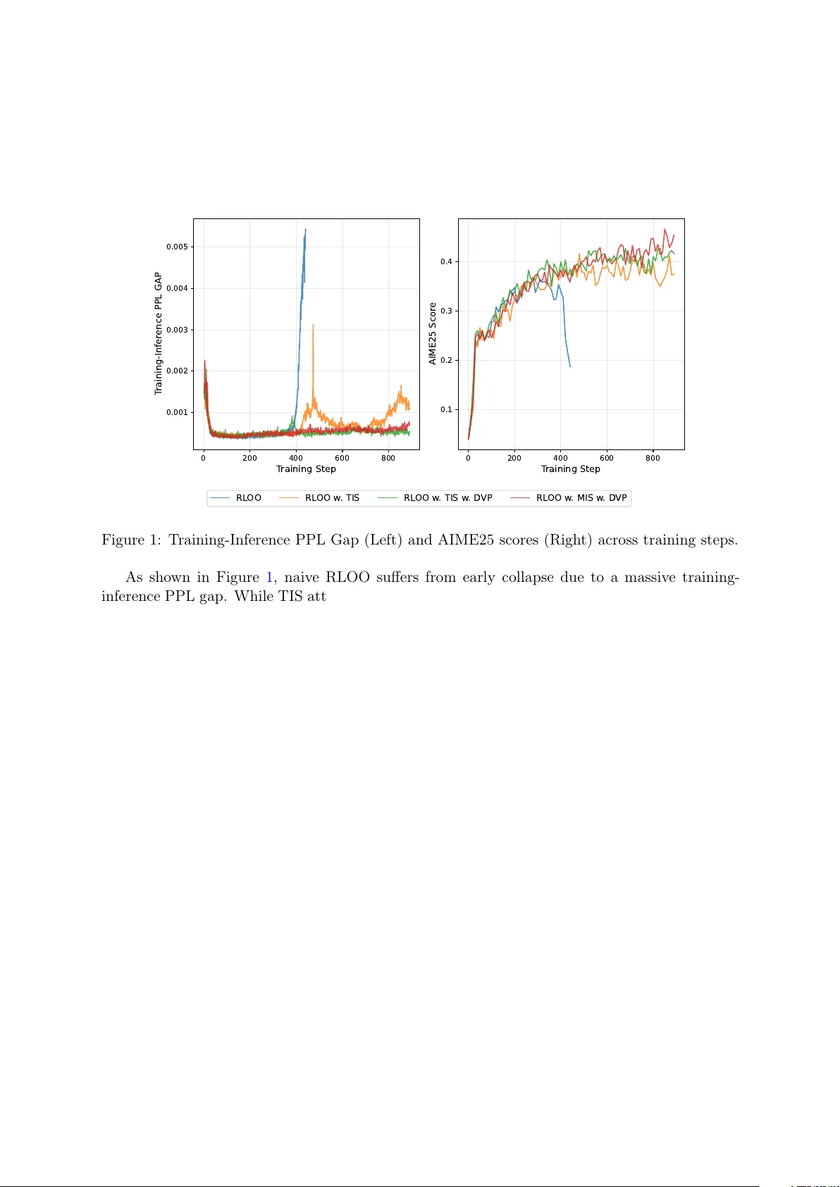
T aming the T ail: Stable LLM Reinforcemen t Learning via Dynamic V o cabulary Pruning ∗ Yingru Li, Jia wei Xu, Jiacai Liu, Y uxuan T ong, Ziniu Li, Tianle Cai, Ge Zhang, Qian Liu, Bao xiang W ang Abstract Reinforcemen t learning for large language mo dels (LLMs) faces a fundamental tension: high-throughput inference engines and n umerically-precise training systems pro duce differen t probabilit y distributions from the same parameters, creating a training-inference mismatch. W e pro ve this mismatc h has an asymmetric effect: the b ound on log-probabilit y mismatch scales as (1 − p ) where p is the token probability . F or high-probability tokens, this bound v anishes, contributing negligibly to sequence-level mismatc h. F or lo w-probability tok ens in the tail, the bound remains large, and moreo ver, when sampled, these tok ens exhibit systematically biased mismatc hes that accum ulate o ver sequences, destabilizing gradien t estimation. Rather than applying post-ho c corrections, w e prop ose constraining the RL ob jective to a dynamically-pruned “safe” vocabulary that excludes the extreme tail. By pruning suc h tokens, w e trade large, systematically biased mismatches for a small, b ounded optimization bias. Empirically , our metho d achiev es stable training; theoretically , we b ound the optimization bias in tro duced by vocabulary pruning. 1 In tro duction 1.1 The Sp eed-Stabilit y Dilemma Reinforcemen t learning has emerged as a k ey tec hnique for training large language mo dels on complex reasoning and m ulti-turn agen tic tasks, where outcome-based rew ards pro vide the pri- mary learning signal. Ho wev er, applying RL to LLMs at scale faces a critical computational b ot- tlenec k: r ol lout gener ation . Pro ducing the large num b er of sample tra jectories needed to estimate p olicy gradients requires high throughput. Mo dern inference engines (e.g., vLLM [ 4 ], SGLang [ 8 ]) ac hieve this through aggressive optimizations including paged attention, low-precision KV-cache (INT8/FP8), and fused CUD A kernels—all designed to maximize tokens p er second. Mean while, training systems (e.g., FSDP , Megatron-LM) must prioritize n umerical stabilit y and gradient precision, t ypically op erating at higher precision (FP32 or mixed precision with careful accumulation). This creates a training-inference mismatch : the inference p olicy π infer θ used to sample tra jectories differs subtly but systematically from the training p olicy π train θ used to compute gradients. One migh t prop ose enforcing iden tical computations across b oth systems. How ever, this defeats the purp ose of using a high-sp eed inference engine, p oten tially reducing throughput b y orders of magnitude. The sp eed-v ersus-consistency tradeoff app ears fundamental: as inference engines become faster through more aggressive optimization, this gap will only widen. T raining instabilit y is therefore not a transient implementation bug but a p ersisten t c hallenge inheren t to the mo dern LLM-RL stack. ∗ First version: Septem b er 8, 2025 1 1.2 Our Approach: Ob jectiv e Redesign ov er Reactive P atc hing This w ork takes a principled stance: w e view training instability not as a tec hnical bug requiring reactiv e correction, but as a symptom of a po orly-sp ecified learning ob jective. Sp ecifically , an y ob jectiv e requiring accurate gradient estimation ov er the extremely lo w-probability tail of a 100,000+ tok en vocabulary is fragile b ecause the log-probability mismatch b ound do es not shrink for low-probabilit y tokens as it do es for high-probability tok ens. W e prop ose a different approac h: redesign the learning ob jective itself to operate only o ver a dynamically-pruned “safe” v o cabulary at each generation step. This achiev es stability by excluding the problematic tail from the ob jective, rather than applying reactiv e patches or ad- ho c clipping after the fact. 1.3 Con tributions Our work mak es three primary con tributions: 1. Rigorous diagnosis : W e c haracterize the mathematical structure of instabilit y in off- p olicy gradien t estimation for LLMs. W e pro v e that vulnerabilit y is asymmetric—the log-probabilit y mismatch b ound scales as (1 − p ) , v anishing for high-probability tok ens but remaining significant for low-probabilit y tokens. Moreov er, we show that sampled low- probabilit y tokens hav e systematically biased mismatches that accumulate o v er sequences (Section 3 ). 2. Principled solution : W e prop ose dynamic v o cabulary pruning using min-p filtering [ 6 ] to define constrained p olicies. This addresses the source of instability at the ob jective lev el rather than through post-ho c corrections (Section 4 ). 3. Empirical v alidation : W e demonstrate that our method ac hieves stable training and significan t p erformance improv emen ts on mathematical reasoning tasks (Section 5 ). 2 Preliminaries W e formalize autoregressiv e text generation as a Marko v Decision Pro cess (MDP). Definition 2.1 (LLM Generation MDP) . The gener ation pr o c ess is define d by: • State : s t = [ x ; y 1 , . . . , y t − 1 ] is the pr ompt x c onc atenate d with tokens gener ate d so far. • A ction : a ∈ V is a token fr om the vo c abulary. • Policy : π θ ( a | s t ) is the LLM’s next-token distribution. • T r aje ctory : y = ( y 1 , . . . , y T ) is a c omplete gener ation. • R ewar d : R ( x, y ) ∈ { 0 , 1 } is typic al ly the c orr e ctness of the solution, applic able to b oth single-turn r e asoning and multi-turn agentic tasks. Standard RL ob jectiv e. The goal is to maximize exp ected reward: J ( θ ) = E y ∼ π θ [ R ( x, y )] . (1) P olicy gradien t. The gradien t is: ∇ θ J ( θ ) = E y ∼ π θ [ ∇ θ log π θ ( y | x ) · R ( x, y )] , (2) where log π θ ( y | x ) = P T t =1 log π θ ( y t | s t ) by the chain rule. The challenge arises when we m ust sample from one p olicy but compute gradien ts with respect to another—the off-p olicy setting underlying the training-inference mismatc h. 2 3 Diagnosis: The F undamen tal Instabilit y T raining instability in LLM reinforcement learning has deep mathematical roots. W e diagnose this instability b y analyzing the training-inference mismatc h scenario. 3.1 The T raining-Inference Mismatc h W e hav e tw o p olicies sharing parameters θ but differing in computational implemen tation: • π train θ : The training p olicy (high precision, used for gradien ts). • π infer θ : The inference p olicy (high sp eed, used for sampling). The ideal gradient uses π train θ for both sampling and gradien t computation. In practice, we sample from π infer θ but compute gradients using π train θ , introducing bias. Theorem 3.1 (Gradien t Bias from Mismatc h) . L et g = E y ∼ π tr ain θ [ ∇ θ log π tr ain θ ( y | x ) · R ( x, y )] b e the ide al gr adient and g ′ = E y ∼ π infer θ [ ∇ θ log π tr ain θ ( y | x ) · R ( x, y )] the pr actic al gr adient. The bias b = g ′ − g satisfies: b = E y ∼ π tr ain θ  (exp( − ∆ y ) − 1) · ∇ θ log π tr ain θ ( y | x ) · R ( x, y )  , (3) wher e ∆ y = log π tr ain θ ( y | x ) − log π infer θ ( y | x ) is the se quenc e-level lo g-pr ob ability mismatch. Pro of in App endix A.1 . The k ey observ ation: the bias magnitude is gov erned by exp( − ∆ y ) = π infer θ ( y ) /π train θ ( y ) , the ratio of sequence probabilities. When ∆ y b ecomes large and negative (meaning π infer θ ( y ) ≫ π train θ ( y ) ), this ratio explo des. While importance sampling can correct for this distributional shift, doing so requires weigh ting samples b y π train θ ( y ) /π infer θ ( y ) —the in verse ratio—whic h b ecomes v anishingly small for the same problematic tra jectories, causing high v ariance. Either wa y , large probabilit y ratios destabilize gradien t estimation. 3.2 Mo deling the Mismatc h: Logit Perturbations T o analyze which tok ens are vulnerable, we must understand ho w the training-inference mis- matc h manifests at the token lev el. Ev en with identical parameters θ , the t w o systems pro duce differen t logits due to a fundamen tal prop ert y of floating-p oin t arithmetic: non-associativity . W e hav e ( a ⊕ b ) ⊕ c  = a ⊕ ( b ⊕ c ) in finite precision, so differen t computation orders yield differen t results [ 3 ]. In practice, inference engines (vLLM [ 4 ], SGLang [ 8 ]) and training frameworks (Megatron- LM, FSDP) differ in m ultiple wa ys: (1) attention implementations —P agedAtten tion [ 4 ] vs. FlashA ttention-2 [ 2 ] use differen t reduction orders for the softmax denominator P j exp( q · k j / √ d ) ; (2) numeric al pr e cision —FP8/INT8 KV-cache quan tization vs. BF16/FP32 accum ula- tion; (3) op er ator fusion —differen t kernel boundaries c hange intermediate rounding. W e mo del the aggregate effect as: z infer = z train + ε , where ε = ( ε 1 , . . . , ε |V | ) (4) represen ts the p erturbation vector. Since these numerical errors arise from b ounded-precision arithmetic, the p erturbations satisfy | ε k | ≤ ϵ max for some small ϵ max . 3.3 Asymmetric V ulnerabilit y With this p erturbation model, we can no w characterize whic h tok ens are most vulnerable. Cru- cially , vulnerability is not uniform across the vocabulary . 3 Prop osition 3.2 (Asymmetric V ulnerabilit y) . Under the lo git p erturb ation mo del z infer = z tr ain + ε with | ε k | ≤ ϵ max , the token-level lo g-pr ob ability mismatch satisfies: | ∆ a | ≤ 2 ϵ max (1 − p a ) , (5) wher e p a = π tr ain θ ( a | s ) is the tr aining p olicy pr ob ability. Pro of in App endix A.2 . This rev eals the asymmetric structure: high-probabilit y tok ens ( p a → 1 ) hav e (1 − p a ) → 0 , so the b ound v anishes; low-probabilit y tokens ( p a → 0 ) hav e (1 − p a ) ≈ 1 , so the b ound remains at its maxim um v alue 2 ϵ max . T o understand the typic al magnitude of mismatch (not just the worst case), we mo del the p erturbations as i.i.d. with mean zero and v ariance σ 2 . Prop osition 3.3 (Signature of F ailure) . Under the p erturb ation mo del with ε k iid ∼ (0 , σ 2 ) , given that action a is sample d fr om π infer θ , the mo de of the mismatch ∆ ′ a = − ∆ a is appr oximately: Mo de [∆ ′ a | a sample d ] ≈ σ 2   (1 − p a )(1 − p ′ a ) + X k  = a p k p ′ k   , (6) wher e p a = π tr ain θ ( a | s ) and p ′ a = π infer θ ( a | s ) . Pro of in App endix A.3 . F or high-probabilit y tok ens, the mo de is near zero (b enign mis- matc h). F or low-probabilit y tokens, the mode is strictly positive, implying the probability ratio π infer θ /π train θ is systematically inflated. This theoretical prediction aligns with prior empirical observ ations: Liu et al. [ 5 ] found that sampled lo w-probability tokens exhibit π infer θ ≫ π train θ in practice, contributing to training collapse. 3.4 Summary The diagnosis is clear: (1) the vocabulary tail is a region of high instability risk; (2) vulnerabilit y is asymmetric—the mismatch b ound v anishes for high-probabilit y toke ns but remains at 2 ϵ max for low-probabilit y tokens; (3) when a low-probabilit y token is sampled, the token-lev el mismatch ∆ a tends to b e negative (Prop osition 3.3 ), meaning π infer θ ( a | s ) ≫ π train θ ( a | s ) . Crucially , these p er-tok en mismatches accum ulate ov er sequences: ∆ y = P t ∆ y t . Sequences containing man y lo w-probability tokens therefore hav e systematically negativ e ∆ y , leading to large sequence-level probabilit y ratios exp( − ∆ y ) ≫ 1 . This motiv ates a solution that excludes the tail from the learning ob jective. 4 Solution: Constrained Optimization via V o cabulary Pruning W e pursue ob jectiv e redesign ov er reactive patching: constrain the learning ob jective to a dynamically-pruned “safe” v o cabulary . 4.1 Dynamic V o cabulary Pruning via Min-P Filtering Min-p sampling [ 6 ] retains tok ens whose probability exceeds a fraction ρ of the maxim um prob- abilit y . W e adapt this for defining safe action sets. Definition 4.1 (Min-P Safe A ction Sets) . Given thr eshold ρ ∈ (0 , 1] , the safe action sets ar e: V S ( s ) =  a ∈ V : π tr ain θ ( a | s ) ≥ ρ · max k π tr ain θ ( k | s )  , (7) V ′ S ( s ) =  a ∈ V : π infer θ ( a | s ) ≥ ρ · max k π infer θ ( k | s )  . (8) The threshold ρ is t ypically extremely small (e.g., ρ = e − 13 ≈ 2 . 3 × 10 − 6 ), retaining a broad set of plausible tok ens while pruning only the extreme tail. 4 4.2 Constrained Policies and Ob jective Definition 4.2 (Min-P Constrained P olicies) . The c onstr aine d p olicies ar e: π tr ain mp ( a | s ) = π tr ain θ ( a | s ) Z θ ( s ) · 1 [ a ∈ V S ( s )] , (9) π infer mp ( a | s ) = π infer θ ( a | s ) Z ′ θ ( s ) · 1 [ a ∈ V ′ S ( s )] , (10) wher e Z θ ( s ) = P k ∈V S ( s ) π tr ain θ ( k | s ) and Z ′ θ ( s ) = P k ∈V ′ S ( s ) π infer θ ( k | s ) . Our constrained RL ob jective is J mp ( θ ) = E y ∼ π train mp [ R ( x, y )] —a differ ent obje ctive from J ( θ ) that av oids the unstable tail b y design. 4.3 The Stable Gradien t Estimator Theorem 4.3 (Constrained Gradien t Estimator) . When sampling y ∼ π infer mp , an estimator of ∇ θ J mp ( θ ) is: ˆ g mp = π tr ain mp ( y | x ) π infer mp ( y | x ) · ∇ θ log π tr ain mp ( y | x ) · R ( x, y ) , (11) wel l-define d whenever y t ∈ V S ( s t ) for al l t . Remark 4.4 (Supp ort Condition) . When y t ∈ V ′ S ( s t ) but y t / ∈ V S ( s t ) , the pr ob ability r atio π tr ain mp /π infer mp is zer o—no bias, just waste d samples. The c onverse c ase (bias-inducing) is r ar e: by Pr op osition 3.2 , high-pr ob ability tokens have smal l | ∆ a | , so π tr ain θ ( a | s ) ≈ π infer θ ( a | s ) , ensuring V S ( s ) ≈ V ′ S ( s ) for tokens that matter. Remark 4.5 (Fixed Safe Sets in Gradient Computation) . W e tr e at V S ( s ) as fixe d during b ack- pr op agation (via torch.no_grad() ), a standar d appr oximation that intr o duc es ne gligible err or. Se e App endix C for implementation details. 4.4 Wh y It W orks: A v oiding Systematic Bias By constraining the ob jectiv e to J mp instead of J , we trade a small optimization bias for stable gradien t estimation. The key b enefit of vocabulary pruning is that it excludes tokens where the mismatch ∆ a is systematically biased. By Prop osition 3.3 , when a lo w-probability tok en is sampled from π infer θ , the mismatch ∆ a tends to be negative, meaning π infer θ ( a | s ) ≫ π train θ ( a | s ) . These systematically negative mismatches accumulate ov er sequences: if many tokens ha ve ∆ y t < 0 , then ∆ y = P t ∆ y t ≪ 0 , causing exp( − ∆ y ) ≫ 1 . By excluding the extreme tail, we a v oid sampling tokens with systematically biased mismatches, prev enting this accum ulation. The optimization bias is b ounded (proof in App endix B ): | J mp ( θ ) − J ( θ ) | ≤ R max · T · (1 − Z min ) , (12) where Z min = min s Z θ ( s ) is the minim um retained probability mass. With ρ = e − 13 , w e ha ve Z θ ( s ) ≈ 1 in nearly all con texts, making the optimization bias negligible. 5 Exp erimen ts W e ev aluate Dynamic V o cabulary Pruning (D VP) on the mathematical reasoning task, emplo ying the RLOO [ 1 ] as the base algorithm. F or our exp erimen tal setup, we utilize the filtered DAPO dataset 1 for training and assess p erformance on the AIME25. W e conduct full 1 https://huggingface.co/datasets/Jiawei415/DPAO_filter/tree/main/train 5 on-p olicy training using the Qw en3-14B-Base, with b oth the rollout batc h size and mini-update size set to 32. The maximum resp onse length is 16,384, and the group size is 16. F or our D VP , we employ a min-p threshold of ρ = e − 13 . F or importance sampling, w e adopt tok en- lev el T runcated Imp ortance Sampling (TIS) [ 7 ] and Masked Imp ortance Sampling (MIS) [ 5 ]. T o mitigate v ariance and ensure repro ducibility , w e rep ort avg@16 scores in Figure 1 . 0 200 400 600 800 T raining Step 0.001 0.002 0.003 0.004 0.005 T raining-Infer ence PPL GAP 0 200 400 600 800 T raining Step 0.1 0.2 0.3 0.4 AIME25 Scor e RL OO RL OO w . TIS RL OO w . TIS w . D VP RL OO w . MIS w . D VP Figure 1: T raining-Inference PPL Gap (Left) and AIME25 scores (Righ t) across training steps. As sho wn in Figure 1 , naiv e RLOO suffers from early collapse due to a massive training- inference PPL gap. While TIS attempts to mitigate this instability , it still exhibits a substan tial PPL gap and fails to ac hiev e competitive results. With DVP , the PPL gap remains stable throughout training, yielding significan tly higher scores. Notably , the com bination of MIS and D VP achiev es a 26.55% improv ement o ver naiv e RLOO’s peak performance. 6 Conclusion W e analyzed training instability in LLM reinforcement learning, sho wing that it arises from distributional mismatc h b etw een inference and training systems. The vulnerability is asymmet- ric: the log-probabilit y mismatch bound scales as (1 − p ) , v anishing for high-probabilit y tokens but remaining large for low-probabilit y tokens. Moreov er, sampled low-probabilit y tokens ha ve systematically biased mismatches that accum ulate o ver sequences, causing sequence-level prob- abilit y ratios to grow large. Rather than applying p ost-hoc corrections, w e prop ose dynamic v o cabulary pruning—constraining the ob jectiv e to a “safe” vocabulary that excludes the ex- treme tail. This av oids tok ens with systematically biased mismatches at the cost of a small, b ounded optimization bias. Our approac h offers a principled path tow ard stable reinforcement learning for LLMs. References [1] A. Ahmadian, C. Cremer, M. Gallé, M. F adaee, J. Kreutzer, O. Pietquin, A. Üstün, and S. Ho ok er. Back to basics: Revisiting reinforce style optimization for learning from human feedbac k in llms. arXiv pr eprint arXiv:2402.14740 , 2024. [2] T. Dao. FlashA ttention-2: F aster attention with better parallelism and work partitioning. arXiv pr eprint arXiv:2307.08691 , 2023. 6 [3] H. He and Thinking Machines Lab. Defeating nondeterminism in LLM inference. Thinking Machines L ab: Conne ctionism , 2025. https://thinkingmachines.ai/blog/ defeating- nondeterminism- in- llm- inference/ . [4] W. Kw on, Z. Li, S. Zh uang, Y. Sheng, L. Zheng, C. H. Y u, J. E. Gonzalez, H. Zhang, and I. Stoica. Efficient memory management for large language model serving with PagedA tten- tion. In Pr o c e e dings of the 29th Symp osium on Op er ating Systems Principles , pages 611–626, 2023. [5] J. Liu, Y. Li, Y. F u, J. W ang, Q. Liu, and Y. Shen. When sp eed kills stability: Demystifying RL collapse from the training-inference mismatch, Sept. 2025. https://richardli.xyz/ rl- collapse . [6] N. N. Minh, A. Bak er, C. Neo, A. G. Roush, A. Kirsc h, and R. Shw artz-Ziv. T urning up the heat: Min-p sampling for creative and coherent LLM outputs. In The Thirte enth International Confer enc e on L e arning R epr esentations , 2025. [7] F. Y ao, L. Liu, D. Zhang, C. Dong, J. Shang, and J. Gao. Y our efficien t rl frame- w ork secretly brings y ou off-policy rl training, Aug. 2025. https://fengyao.notion.site/ off- policy- rl . [8] L. Zheng, L. Yin, Z. Xie, C. Sun, J. Huang, C. H. Y u, S. Cao, C. Kober, Y. Sheng, J. E. Gonzalez, I. Stoica, and H. Zhang. SGLang: Efficient execution of structured language mo del programs. arXiv pr eprint arXiv:2312.07104 , 2024. 7 A Pro ofs A.1 Pro of of Theorem 3.1 : Gradient Bias Pr o of. T ransform g ′ b y imp ortance sampling: g ′ = E y ∼ π infer θ [ ∇ θ log π train θ ( y | x ) · R ( x, y )] (13) = E y ∼ π train θ  π infer θ ( y | x ) π train θ ( y | x ) · ∇ θ log π train θ ( y | x ) · R ( x, y )  (14) = E y ∼ π train θ  exp( − ∆ y ) · ∇ θ log π train θ ( y | x ) · R ( x, y )  . (15) Th us b = g ′ − g = E y ∼ π train θ  (exp( − ∆ y ) − 1) · ∇ θ log π train θ ( y | x ) · R ( x, y )  . A.2 Pro of of Prop osition 3.2 : Asymmetric V ulnerability Pr o of. Let z ′ = z + ε b e perturb ed logits with | ε k | ≤ ϵ max . Define f a ( z ) = log softmax ( z ) a = z a − log P j e z j . By the Mean V alue Theorem: ∆ a = f a ( z ) − f a ( z ′ ) = −∇ f a ( z c ) · ε for some z c . The gradient is ∂ f a ∂ z k = δ ak − p k ( z c ) . Therefore: − ∆ a = (1 − p a ( z c )) ε a − X k  = a p k ( z c ) ε k . (16) By the triangle inequalit y: | ∆ a | ≤ ϵ max   (1 − p a ( z c )) + X k  = a p k ( z c )   = 2 ϵ max (1 − p a ( z c )) . (17) A.3 Pro of of Prop osition 3.3 : Signature of F ailure Pr o of. Let E a denote “action a sampled from π infer θ .” Using Ba yes’ theorem with Gaussian prior on p erturbations: log P ( ε | E a ) = ( z a + ε a ) − log X j e z j + ε j − 1 2 σ 2 X j ε 2 j + const . (18) Setting deriv ativ es to zero: ε ∗ k = σ 2 ( δ ak − p ′ k ) . Substituting into ∆ ′ a = − ∆ a ≈ (1 − p a ) ε a − P k  = a p k ε k : Mo de [∆ ′ a | E a ] = σ 2   (1 − p a )(1 − p ′ a ) + X k  = a p k p ′ k   . (19) B Bias-V ariance Analysis Details B.1 Con trastiv e Gradien t F orm Prop osition B.1 (Con trastive Gradien t Decomp osition) . F or a ∈ V S ( s ) : ∇ θ log π tr ain mp ( a | s ) = ∇ θ log π tr ain θ ( a | s ) − E k ∼ π tr ain mp [ ∇ θ log π tr ain θ ( k | s )] . (20) 8 Pr o of. F rom log π train mp ( a | s ) = log π train θ ( a | s ) − log Z θ ( s ) : ∇ θ log π train mp ( a | s ) = ∇ θ log π train θ ( a | s ) − P k ∈V S π train θ ( k | s ) ∇ θ log π train θ ( k | s ) Z θ ( s ) (21) = ∇ θ log π train θ ( a | s ) − E k ∼ π train mp [ ∇ θ log π train θ ( k | s )] . (22) Expressing in terms of logits z a : b oth standard and constrained gradien ts ha ve the form ∇ θ z a − b , where the baseline b is an exp ectation ov er the resp ectiv e distribution. The constrained baseline is fo cused on relev ant tok ens rather than diluted across 100,000+ tail tok ens. B.2 Pro of of Bias Bound Pr o of. By total v ariation b ounds: | E P [ f ] − E Q [ f ] | ≤ ∥ f ∥ ∞ · TV ( P, Q ) . F or tra jectory distributions: TV( π train mp , π train θ ) ≤ P T t =1 E s t [TV( π train mp ( ·| s t ) , π train θ ( ·| s t ))] . F or a single step: TV( π train mp ( ·| s ) , π train θ ( ·| s )) = 1 2 X a | π train mp ( a | s ) − π train θ ( a | s ) | (23) = 1 2 [(1 − Z θ ( s )) + (1 − Z θ ( s ))] = 1 − Z θ ( s ) . (24) Th us | J mp − J | ≤ R max · P t E s t [1 − Z θ ( s t )] ≤ R max · T · (1 − Z min ) . C Implemen tation Details C.1 Logit Masking The constrained policy π train mp in volv es selecting the safe set V S ( s ) , a non-differen tiable op eration. W e show that simple logit masking correctly implements the required gradient. Define masked logits: z mp ,k = ( z k if k ∈ V S ( s ) −∞ otherwise . (25) Prop osition C.1 (Mask ed Logit Correctness) . F or al l a ∈ V S ( s ) : 1. softmax ( z mp ) a = π tr ain mp ( a | s ) . 2. ∇ θ log( softmax ( z mp ) a ) = ∇ θ log π tr ain mp ( a | s ) , tr e ating V S ( s ) as fixe d. Pr o of. P art 1 (P olicy equiv alence): softmax ( z mp ) a = e z mp ,a P j e z mp ,j (26) = e z a P k ∈V S ( s ) e z k + P l / ∈V S ( s ) e −∞ (27) = e z a P k ∈V S ( s ) e z k = π train θ ( a | s ) Z θ ( s ) = π train mp ( a | s ) . (28) P art 2 (Gradient equiv alence): T reating V S ( s ) as fixed, the gradien t of log-softmax is ∇ θ z a − E k ∼ softmax ( z mp ) [ ∇ θ z k ] . Since softmax ( z mp ) = π train mp , this equals ∇ θ z a − E k ∼ π train mp [ ∇ θ z k ] = ∇ θ log π train mp ( a | s ) . 9 C.2 PyT orch Implemen tation 1 i m p o r t m a t h 2 i m p o r t t o r c h 3 4 d e f a p p l y _ m i n p _ m a s k i n g ( l o g i t s , r h o = m a t h . e x p ( - 1 3 ) , m a s k _ v a l u e = - 5 0 . 0 ) : 5 " " " 6 A p p l y m i n - p m a s k i n g t o l o g i t s . 7 8 S a f e s e t : V _ S ( s ) = { a | p i ( a | s ) > = p i _ m a x ( s ) * r h o } 9 E q u i v a l e n t i n l o g i t s p a c e : l o g i t ( a ) > = l o g i t _ m a x + l o g ( r h o ) 10 11 A r g s : 12 l o g i t s : L o g i t s t e n s o r ( . . . , v o c a b _ s i z e ) 13 r h o : M i n - p t h r e s h o l d ( d e f a u l t : e ^ { - 1 3 } ) 14 m a s k _ v a l u e : V a l u e f o r m a s k e d l o g i t s ( - 5 0 . 0 i s s a f e f o r B F 1 6 ) 15 " " " 16 w i t h t o r c h . n o _ g r a d ( ) : 17 # S a f e s e t : l o g i t > = l o g i t _ m a x + l o g ( r h o ) 18 t h r e s h o l d = l o g i t s . m a x ( d i m = - 1 , k e e p d i m = T r u e ) . v a l u e s + m a t h . l o g ( r h o ) 19 m a s k = l o g i t s < t h r e s h o l d 20 r e t u r n t o r c h . w h e r e ( m a s k , m a s k _ v a l u e , l o g i t s ) Listing 1: Min-p masking implementation. C.3 Key Implementation Details 1. Mask creation in no_grad() con text : The selection of V S ( s ) happ ens inside torch.no_grad() , implemen ting the fixed safe set approximation (Remark 4.5 ). 2. Logit-space threshold : W e compute the threshold as z max + log( ρ ) to av oid numerical issues with small probabilities. 3. Mask v alue : The mask v alue − 50 . 0 is effectively zero after softmax but a voids NaN gradien ts in mixed-precision (BF16) training. 4. Gradien t-safe masking : W e use torch.where instead of in-place masked_fill_ for a cleaner computation graph. 5. Imp ortance w eight computation : The ratio π train mp ( y ) /π infer mp ( y ) is computed b y get- ting log-probabilities from b oth training and inference systems and exponentiating their difference. C.4 Choice of ρ The threshold ρ con trols the bias-v ariance tradeoff: • Larger ρ : More aggressive pruning, smaller safe set, lo wer v ariance but higher bias. • Smaller ρ : Less aggressiv e pruning, larger safe set, low er bias but less v ariance reduction. In our exp erimen ts, w e use ρ = e − 13 ≈ 2 . 26 × 10 − 6 , which prunes the extreme tail while retaining sufficient div ersit y for mathematical reasoning. 10