FEM-Bench: A Structured Scientific Reasoning Benchmark for Evaluating Code-Generating LLMs

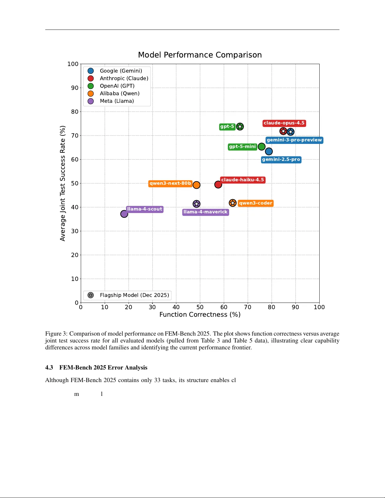
F E M - B E N C H : A S T R U C T U R E D S C I E N T I FI C R E A S O N I N G B E N C H M A R K F O R E V A L U A T I N G C O D E - G E N E R A T I N G L L M S A P R E P R I N T Saeed Mohammadzadeh ∗ Department of Mechanical Engineering Boston Univ ersity Boston, MA saeedmhz@bu.edu Erfan Hamdi ∗ Department of Mechanical Engineering Boston Univ ersity Boston, MA erfan@bu.edu Joel Shor 1. Move37 Labs 2. Department of Mechanical Engineering, Boston Univeristy joel.shor@move37labs.ai Emma Lejeune Department of Mechanical Engineering Boston Univ ersity Boston, MA elejeune@bu.edu December 25, 2025 A B S T R AC T As LLMs advance their reasoning capabilities about the ph ysical world, the absence of rigorous benchmarks for ev aluating their ability to generate scientiﬁcally v alid physical models has become a critical g ap. Computational mechanics, the discipline that de velops and applies mathematical mod- els and numerical methods to predict the behavior of physical systems under forces, deformation, and constraints, provides an ideal foundation for structured scientiﬁc reasoning based ev aluation. Problems follo w clear mathematical structure, enforce strict physical and numerical constraints, and support objective veriﬁcation. The discipline also requires constructing explicit models of physical systems and reasoning about geometry , spatial relationships, and material behavior , which connects directly to emerging goals in AI related to physical reasoning and world modeling. W e introduce FEM-Bench, a computational mechanics benchmark designed to ev aluate the ability of LLMs to generate correct ﬁnite element method (FEM) and related code. FEM-Bench 2025 contains a suite of introductory but nontri vial tasks aligned with material from a ﬁrst graduate course on computa- tional mechanics. These tasks capture essential numerical and physical modeling challenges while representing only a small fraction of the complexity present in the discipline. Despite their simplic- ity , state-of-the-art LLMs do not reliably solv e all of them. In a ﬁv e attempt run, the best performing model at function writing, Gemini 3 Pro, completed 30/33 tasks at least one out of ﬁ ve times, and 26/33 tasks ﬁv e out of ﬁv e times. The best performing model at unit test writing, GPT -5, had an A verage Joint Success Rate of 73.8%. Other popular models showed a broad range of performance on the benchmark. FEM-Bench establishes a structured foundation for ev aluating AI-generated sci- entiﬁc code, and future iterations will incorporate increasingly sophisticated tasks to track progress as models ev olve. Keyw ords Lar ge Language Models (LLMs) · Finite Element Method (FEM) · LLM Benchmark · Scientiﬁc Machine Learning · Computational Mechanics · Scientiﬁc Computing · Code Generation ∗ Saeed Mohammadzadeh and Erf an Hamdi are co-ﬁrst authors FEM-Bench 2025 A P R E P R I N T 1 Introduction Modern AI systems are increasingly evaluated on their ability to build internal models of the physical w orld, including reasoning about forces, geometry , spatial relationships, and the mechanical behavior of physical systems [Bakhtin et al., 2019, W ang et al., 2023]. Simultaneously , lar ge language models (LLMs) show gro wing potential to assist with scientiﬁc and engineering w orkﬂows, including reasoning about physical systems and automated generation of simu- lation and analysis code [Cui et al., 2025]. As these models advance, a central question emerges: can LLMs produce implementations of physics-based numerical methods that are correct, reliable, and scientiﬁcally meaningful? Existing code-generation benchmarks test general programming logic [Austin et al., 2021a, Chen et al., 2021a], software engi- neering skills [Jimenez et al., 2023], and mathematical reasoning [Glazer et al., 2024], but no widely used benchmarks ev aluate an LLMs ability to carry out the physical modeling, numerical discretization, and structured computational reasoning required for advanced scientiﬁc computing [Tian et al., 2024]. Computational mechanics, the discipline that formulates and solves mathematical models of physical systems using numerical methods, provides a natural and rigorous domain in which to in vestigate these capabilities. Computational-mechanicsbased tasks represent a particularly important frontier for LLM capabilities [Jiang et al., 2025]. Physics-based simulations grounded in this discipline underpin real-world applications in domains as di verse as robotics [Huang et al., 2020], digital twins of aircraft and human systems [Niederer et al., 2021], climate model- ing [Danabasoglu et al., 2020], and engineering design and optimization [T alischi et al., 2012]. Across these areas, sev eral themes are consistent: successful simulation requires the seamless integration of mathematics, physics, ge- ometry , numerical methods, and programming, and correctness is non-ne gotiable. A program that runs b ut produces a non-con ver gent, unstable, or physically impossible result is of no scientiﬁc value [Peng, 2011]. For this reason, computational mechanics has a long and mature tradition of veriﬁcation, v alidation, and uncertainty quantiﬁcation [Oberkampf and Roy, 2010], providing structured, quantitative tools for assessing whether a model is numerically consistent, physically plausible, and predictive. These practices make the domain especially well-suited for ev aluating LLM-generated code, because failures are interpretable, quantitativ ely measurable, and can be traced not only to pro- gramming or structural errors but also to deeper mistak es in implementing gov erning equations, enforcing numerical consistency , handling geometric transformations, or managing ﬂoating-pointsensiti ve operations such as numerical integration and matrix assembly [Arndt et al., 2023, Alnæs et al., 2015]. Thus, this branch of scientiﬁc computing provides a well-structured and scientiﬁcally grounded testbed for critically ev aluating the emer ging capabilities of LLMs. Problems in computational mechanics follow a precise mathematical pipeline: e.g., governing equations are formulated, con verted into weak or variational forms, discretized into ﬁnite- dimensional approximations, and assembled into global algebraic systems [Courant et al., 1994, T urner et al., 1956]. Solutions are then v alidated through objectiv e numerical checks such as symmetry , consistency , and mesh con ver gence [Zienkiewicz and T aylor, 1997]. From the perspecti ve of LLM reasoning, these tasks span multiple forms of structured cognition: hierarchical reasoning in which local element routines combine into global models; geometric transforma- tions across coordinate systems; the construction of explicit models of physical systems; and careful handling of numerical integration, stability , and ﬂoating-pointsensitive operations. Moreover , the computational mechanics litera- ture is e xtensiv e and mature. The computational mechanics literature spans classic textbooks [Hughes, 2003], widely taught graduate curricula in engineering [Garikipati, 2015, Shojaei et al., 2025], and ongoing research at the frontier of numerical methods dev elopment [Kamarei et al., 2026], offering a rich, well-understood space of problems with clear expectations for correctness and implementation quality [Szabó and Bab uška, 2021]. In this work, we introduce FEM-Bench, a benchmark designed to e valuate the ability of LLMs to generate correct im- plementations of ﬁnite element method (FEM) and related computational mechanics tasks. FEM-Bench 2025 focuses on introductory but nontrivial tasks aligned with material from a ﬁrst graduate course on FEM. These tasks isolate es- sential numerical and physical modeling challenges while remaining amenable to automated ev aluation. Despite their relativ e simplicity , we ﬁnd that state-of-the-art LLMs show signiﬁcant room for improv ement, re vealing signiﬁcant gaps between current model capabilities and the requirements of physics-based scientiﬁc computing. The contrib utions of this paper are threefold. First, we present the FEM-Bench framew ork, including its design prin- ciples and scope. Second, we provide a suite of tasks and corresponding ev aluation tools grounded in canonical computational mechanics concepts. Third, we conduct a baseline ev aluation across several leading LLMs to char- acterize current performance. Looking forward, FEM-Bench establishes a foundation for increasingly challenging computational mechanics tasks in future iterations, enabling systematic tracking of progress in scientiﬁc computing speciﬁc code generation. 2 FEM-Bench 2025 A P R E P R I N T 2 Background This Section provides background on computational mechanics as a domain for ev aluating LLMs, emphasizing physi- cal grounding, algorithmic structure, and rigorous veriﬁcation culture. W e then motiv ate the need for FEM-Bench as a benchmark designed to probe these capabilities in a scientiﬁcally meaningful setting. 2.1 Computational Mechanics as a T est of Physical W orld Modeling Computational mechanics provides the mathematical and numerical foundation for simulating the behavior of physical systems under forces, deformation, and constraints [Belytschko et al., 2014, Gurtin et al., 2010]. At its core, the ﬁeld translates ph ysical laws into solv able mathematical models, which are then discretized and implemented as algorithms suitable for computation [Langtangen, 2003]. In doing so, computational mechanics serves as a direct test of whether a model can correctly represent and reason about the physical world in algorithmic form. Among the many techniques used in computational mechanics, the Finite Element Method (FEM) and Matrix Structural Analysis (MSA) are two of the most widely taught and broadly applied approaches [Hughes, 2003, McGuire et al., 2000]. MSA predates FEM and was originally de veloped to analyze framed structures such as trusses and beams using stif fness matrices deri ved directly from structural mechanics [Argyris et al., 1960, T urner et al., 1956]. Although more specialized in scope, MSA shares the same foundational principles as FEMlocal element stiffness relations, coordinate transformations, and global assemblyand is often viewed as an early , specialized precursor to the broader ﬁnite element frame work [Cook et al., 2007]. These shared ideas make MSA a natural companion to FEM in introductory mechanics curricula and a relev ant component of the FEM-Bench task space [Felippa, 2004]. (ii) Discre  za  on with the  nite element me thod (FEM) (i) Solid mechanics problem: Giv en loads and boundary condi  ons solve f or def orma  on Figure 1: Schematic overvie w of the ﬁnite element method (FEM). (i) A solid mechanics problem: giv en loads and boundary conditions on the reference conﬁguration, solve for the deformation mapping to the deformed conﬁguration. (ii) Discretization step: the continuous domain is approximated by a mesh of ﬁnite elements and nodes, enabling numerical solution of the relev ant gov erning equations. 3 FEM-Bench 2025 A P R E P R I N T 2.2 Computational Mechanics as a T est of Structured, Multistep Reasoning At a high le vel, FEM proceeds through a well-deﬁned sequence of modeling steps. Each step depends on the correct ex ecution of preceding stages, requiring careful composition of intermediate representations and computations. As il- lustrated in Fig. 1 , a continuous physical domain is ﬁrst subdivided into a ﬁnite mesh of elements. Physical gov erning equations are expressed in a weak or variational form, enabling approximate solutions in ﬁnite-dimensional function spaces [Strang et al., 1973]. On each element, basis (or shape) functions deﬁne ho w the unkno wn ﬁeld varies locally , and numerical quadrature is used to ev aluate inte grals appearing in the weak form [Hughes, 2003, Press, 2007]. These element-lev el contributions are then assembled into a global algebraic system whose solution approximates the physi- cal equilibrium state or transient ev olution of the system [Bathe, 1996]. A schematic illustration of the discretization appears in Fig. 1 . This mathematical pipeline is central to nearly all engineering simulation softw are and forms the conceptual backbone of FEM-Bench. The mechanics tasks underlying FEM, and by e xtension MSA, in v olve sev eral forms of structured computational rea- soning that are highly rele v ant for e v aluating modern LLMs [T ian et al., 2024]. Hierarchical reasoning is required be- cause global beha vior emerges from local element routines combined through assembly operators [Arndt et al., 2023]. Geometric reasoning appears through coordinate transformations, Jacobians, and mappings between reference and global coordinate systems [Cottrell et al., 2009]. Numerical reasoning arises through quadrature rules, element stif f- ness deriv ations, matrix assembly , stability considerations, and ﬂoating-pointsensitiv e calculations [Higham, 2002]. Finally , physical reasoning is inherent to the discipline: implementations must faithfully encode conservation laws, constitutiv e relations, and boundary conditions [Holzapfel, 2002]. These components appear ev en in introductory FEM tasks, making the domain particularly suitable for probing LLM capabilities in scientiﬁc computing. 2.3 V eriﬁcation and Evaluation in Computational Mechanics An essential pillar of computational mechanics, equally relev ant for benchmarking, is its strong culture of v eriﬁcation, validation, and uncertainty quantiﬁcation (VVUQ) [Oberkampf and Roy, 2010]. These practices transform numerical implementations into testable artifacts with well-deﬁned correctness criteria, making them particularly suitable for diagnostic e v aluation. Because simulation outputs must reﬂect real physical beha vior , the ﬁeld has de veloped rigorous practices for assessing correctness, including patch tests, equilibrium checks, symmetry requirements, energy consis- tency , and mesh con v ergence studies [Belytschko et al., 2014, Cook et al., 2007, Macneal and Harder, 1985, Roache, 1998]. These methods provide objectiv e, quantitativ e signals of whether an implementation is functioning correctly . For ev aluating LLM-generated code, such tests are especially valuable: they make failures interpretable and help dis- tinguish mistakes in programming logic [Ammann and Offutt, 2017], geometry handling [Foley, 1996], numerical implementation [T refethen and Bau, 2022], or ﬂoating-pointsensitive operations such as numerical integration and matrix assembly [Higham, 2002]. 2.4 Motivation f or FEM-Bench The broader landscape of existing LLM benchmarks highlights the need for a physics-based alternativ e. Popular code- generation benchmarks such as HumanEv al [Chen et al., 2021b], MBPP [Austin et al., 2021b], SWE-Bench [Jimenez et al., 2024], and DS-1000 [Lai et al., 2022] ev aluate programming logic, tool use, or general software engineering skills. Datasets targeting physical reasoning often focus on qualitativ e judgments or simpliﬁed en vironments rather than implementation of scientiﬁc algorithms [Hamdi and Lejeune, 2026, Lejeune, 2020, Shor et al., 2025]. Like wise, benchmarks for mathematics [Hendrycks et al., 2021] or symbolic reasoning [Mirzadeh et al., 2025] do not require translating equations into stable, reliable numerical code. While recent efforts like FEABench [Mudur et al., 2024] introduce agent-based tasks that interact with professional simulation software, they primarily measure the ability to navigate complex software APIs and external tools; this highlights a critical need to decouple the interpretation of software documentation from the actual implementation of the underlying physical and numerical reasoning. As a result, there is a limited availability of benchmarks to e valuate whether LLMs can generate the kinds of physics- grounded, numerically consistent programs that underpin modern scientiﬁc computing [T ian et al., 2024]. Computational mechanics therefore provides both the conceptual structure and the ev aluati ve tools needed for such an assessment [Oberkampf and Roy, 2010]. Its combination of mathematical rigor , geometric comple xity , numerical precision, and physical grounding makes it an ideal basis for the de velopment of FEM-Bench [Hughes, 2003, McGuire et al., 2000]. In short, FEM-Bench simultaneously tests a collection of general-purpose, high-v alue LLM capabilities that rarely naturally occur together: self-v eriﬁcation , multi-step r easoning , algorithmic ﬁdelity , and memorization . In the next section, we introduce the benchmark design and describe the task suite that forms the FEM-Bench 2025 release. 4 FEM-Bench 2025 A P R E P R I N T 3 Methods This Section describes the FEM-Bench methodology , including the structure of the benchmark, the construction of tasks and prompts, the e valuation pipeline for code and test generation, and the initial selection of LLMs to ev aluate. FEM-Bench follows a modular design: tasks are deﬁned as self-contained Python modules, prompts are generated automatically from task metadata, LLM outputs are parsed and validated, and results are computed through reference- based numerical and unit-testing procedures. The framew ork is designed for reproducibility , extensibility , and prin- cipled e valuation. A high-lev el ov erview of the FEM-Bench workﬂow , including task loading, prompt generation, model inference, and ev aluation, is sho wn in Fig. 2. core FEM-Bench software load tasks write prompts load LLM code evaluate LLM code + tests score LLM code + tests tasks LLM API calls study results LLM generated code + tests prompts for code + tests Figure 2: Overview of the FEM-Bench workﬂo w . T asks are deﬁned as self-contained Python modules specifying reference implementations, dependencies, and unit tests. The core FEM-Bench software loads these tasks, constructs standardized prompts for both code-generation and test-generation, and interfaces with LLMs through model-speciﬁc API clients. LLM outputs (generated code and test suites) are then parsed, validated, and e valuated using reference- based numerical checks and e xpected-failure unit tests. The framew ork produces detailed scores for each model and task, enabling reproducible and interpretable comparison of LLM performance. 3.1 Problem Deﬁnition FEM-Bench ev aluates two complementary capabilities of LLMs: the ability to generate numerically correct scientiﬁc code, and the ability to generate unit tests that verify that code. In this benchmark, producing correct code means generating a Python function that conforms to a prescribed signature, runs without syntax errors, and returns outputs that satisfy the mathematical and physical requirements of the task. Similarly , producing a correct unit test means generating tests written using pytest , a widely used Python testing framework, that ex ecute without errors, pass on the reference implementation, and fail on a curated set of kno wn incorrect implementations. Because scientiﬁc software correctness depends as much on veriﬁcation as on implementation, FEM-Bench treats code synthesis and test synthesis as intertwined, ﬁrst-class components of the benchmark. T ogether, these two components deﬁne the core problem that FEM-Bench poses to LLMs: not simply producing code that runs, but producing code and unit tests that are technically correct. 3.2 T ask Deﬁnition and Structure FEM-Bench deﬁnes each task as a self-contained Python module with a standardized, explicit structure designed for transparency , reproducibility , and extensibility . Every task includes: a reference implementation with a detailed docstring (which becomes part of the LLM prompt), Pytest-style test functions with descriptiv e docstrings (also incor - porated directly into the prompt), optional dependency functions, known incorrect implementations used as expected failures, and a single task_info() function. The task_info() function assembles these components into a structured 5 FEM-Bench 2025 A P R E P R I N T dictionary that contains all metadata and source code required for prompt generation, e xecution, and ev aluation. This “source-ﬁrst” design ensures that tasks remain fully executable and easy to inspect or extend. The full task template is shown in Listing 1 . Listing 1: FEM-Bench task template i m p o r t n u m p y a s n p # = = = D e p e n d e n c y f u n c t i o n s ( i f a n y ) = = = d e f h e l p e r _ 1 ( . . . ) : . . . d e f h e l p e r _ 2 ( . . . ) : . . . # = = = R e f e r e n c e i m p l e m e n t a t i o n = = = d e f m a i n _ f c n ( . . . ) : " " " C o m p u t e o r s o l v e s o m e t h i n g . " " " . . . # = = = T e s t f u n c t i o n s = = = d e f t e s t _ c a s e _ 1 ( f c n ) : " " " D o c s t r i n g e x p l a i n i n g w h a t i s t e s t e d . " " " . . . # = = = K n o w n f a i l i n g e x a m p l e s ( o p t i o n a l ) = = = d e f f a i l _ c a s e _ 1 ( . . . ) : . . . d e f f a i l _ c a s e _ 2 ( . . . ) : . . . # = = = t a s k _ i n f o ( ) m e t a d a t a = = = d e f t a s k _ i n f o ( ) : t a s k _ i d = " u n i q u e _ t a s k _ n a m e " t a s k _ s h o r t _ d e s c r i p t i o n = " c o n c i s e d e s c r i p t i o n o f w h a t t h e t a s k d o e s " c r e a t e d _ d a t e = " Y Y Y Y - M M - D D " c r e a t e d _ b y = " y o u r _ n a m e " m a i n _ f c n = m a i n _ f c n r e q u i r e d _ i m p o r t s = [ " i m p o r t n u m p y a s n p " , " i m p o r t p y t e s t " , # a d d i t i o n a l i m p o r t s i f n e e d e d ] f c n _ d e p e n d e n c i e s = [ h e l p e r _ 1 , h e l p e r _ 2 ] # o r [ ] i f n o n e r e f e r e n c e _ v e r i f i c a t i o n _ i n p u t s = [ # L i s t o f l i s t s : e a c h s u b l i s t c o n t a i n s a r g s f o r m a i n _ f c n [ a r g 1 , a r g 2 , . . . ] , . . . ] t e s t _ c a s e s = [ { " t e s t _ c o d e " : t e s t _ c a s e _ 1 , " e x p e c t e d _ f a i l u r e s " : [ f a i l _ c a s e _ 1 , f a i l _ c a s e _ 2 ] # o r [ ] } , . . . ] r e t u r n { " t a s k _ i d " : t a s k _ i d , " t a s k _ s h o r t _ d e s c r i p t i o n " : t a s k _ s h o r t _ d e s c r i p t i o n , " c r e a t e d _ d a t e " : c r e a t e d _ d a t e , " c r e a t e d _ b y " : c r e a t e d _ b y , 6 FEM-Bench 2025 A P R E P R I N T " m a i n _ f c n " : m a i n _ f c n , " r e q u i r e d _ i m p o r t s " : r e q u i r e d _ i m p o r t s , " f c n _ d e p e n d e n c i e s " : f c n _ d e p e n d e n c i e s , " r e f e r e n c e _ v e r i f i c a t i o n _ i n p u t s " : r e f e r e n c e _ v e r i f i c a t i o n _ i n p u t s , " t e s t _ c a s e s " : t e s t _ c a s e s , " a l l o w _ n e g a t i o n _ f o r _ m a t c h " : F a l s e , " p y t h o n _ v e r s i o n " : " v e r s i o n _ n u m b e r " , " p a c k a g e _ v e r s i o n s " : { " n u m p y " : " v e r s i o n " } , } When a task is loaded, FEM-Bench extracts and normalizes the source code for the reference function, helpers, and tests, and stores them in a Task object deﬁned in task_base.py . This object provides the canonical representation of the task throughout the remainder of the pipeline, including prompt construction, LLM inference, and ev aluation. 3.2.1 Example T ask T o ground this template in a concrete example, Listing 2 shows an actual FEM-Bench task from the FEM-Bench 2025 suite. This task deﬁnes the local 12 × 12 elastic stiffness matrix for a 3D Euler–Bernoulli beam element, along with two pytest-style test functions. The ﬁrst test ( test_local_stiffness_3D_beam ) checks structural properties such as symmetry , rigidity , and consistency of axial, torsional, and bending terms. The second test ( test_cantilever_deflection_matches_euler_bernoulli ) compares numerical displacements with closed-form Euler–Bernoulli beam theory under dif ferent loading directions. The task_info() function then packages the refer- ence implementation, veriﬁcation inputs, and expected-failure implementations into the standardized FEM-Bench task format. Listing 2: Example FEM-Bench task: local stiffness matrix for a 3D Euler–Bernoulli beam element. i m p o r t n u m p y a s n p d e f M S A _ 3 D _ l o c a l _ e l a s t i c _ s t i f f n e s s _ C C 0 _ H 0 _ T 0 ( E : f l o a t , n u : f l o a t , A : f l o a t , L : f l o a t , I y : f l o a t , I z : f l o a t , J : f l o a t ) - > n p . n d a r r a y : " " " R e t u r n t h e 1 2 Œ 1 2 l o c a l e l a s t i c s t i f f n e s s m a t r i x f o r a 3 D E u l e r - B e r n o u l l i b e a m e l e m e n t . T h e b e a m i s a s s u m e d t o b e a l i g n e d w i t h t h e l o c a l x - a x i s . T h e s t i f f n e s s m a t r i x r e l a t e s l o c a l n o d a l d i s p l a c e m e n t s a n d r o t a t i o n s t o f o r c e s a n d m o m e n t s u s i n g t h e e q u a t i o n : [ f o r c e _ v e c t o r ] = [ s t i f f n e s s _ m a t r i x ] @ [ d i s p l a c e m e n t _ v e c t o r ] D e g r e e s o f f r e e d o m a r e o r d e r e d a s : [ u 1 , v 1 , w 1 , x 1 , y 1 , z 1 , u 2 , v 2 , w 2 , x 2 , y 2 , z 2 ] W h e r e : - u , v , w : d i s p l a c e m e n t s a l o n g l o c a l x , y , z - x , y , z : r o t a t i o n s a b o u t l o c a l x , y , z - S u b s c r i p t s 1 a n d 2 r e f e r t o n o d e i a n d n o d e j o f t h e e l e m e n t P a r a m e t e r s : E ( f l o a t ) : Y o u n g ’ s m o d u l u s n u ( f l o a t ) : P o i s s o n ’ s r a t i o ( u s e d f o r t o r s i o n o n l y ) A ( f l o a t ) : C r o s s - s e c t i o n a l a r e a L ( f l o a t ) : L e n g t h o f t h e b e a m e l e m e n t I y ( f l o a t ) : S e c o n d m o m e n t o f a r e a a b o u t t h e l o c a l y - a x i s 7 FEM-Bench 2025 A P R E P R I N T I z ( f l o a t ) : S e c o n d m o m e n t o f a r e a a b o u t t h e l o c a l z - a x i s J ( f l o a t ) : T o r s i o n a l c o n s t a n t R e t u r n s : n p . n d a r r a y : A 1 2 Œ 1 2 s y m m e t r i c s t i f f n e s s m a t r i x r e p r e s e n t i n g a x i a l , t o r s i o n a l , a n d b e n d i n g s t i f f n e s s i n l o c a l c o o r d i n a t e s . " " " k _ e = n p . z e r o s ( ( 1 2 , 1 2 ) ) # A x i a l t e r m s - e x t e n s i o n o f l o c a l x a x i s a x i a l _ s t i f f n e s s = E * A / L k _ e [ 0 , 0 ] = a x i a l _ s t i f f n e s s k _ e [ 0 , 6 ] = - a x i a l _ s t i f f n e s s k _ e [ 6 , 0 ] = - a x i a l _ s t i f f n e s s k _ e [ 6 , 6 ] = a x i a l _ s t i f f n e s s # T o r s i o n t e r m s - r o t a t i o n a b o u t l o c a l x a x i s t o r s i o n a l _ s t i f f n e s s = E * J / ( 2 . 0 * ( 1 + n u ) * L ) k _ e [ 3 , 3 ] = t o r s i o n a l _ s t i f f n e s s k _ e [ 3 , 9 ] = - t o r s i o n a l _ s t i f f n e s s k _ e [ 9 , 3 ] = - t o r s i o n a l _ s t i f f n e s s k _ e [ 9 , 9 ] = t o r s i o n a l _ s t i f f n e s s # B e n d i n g t e r m s - b e n d i n g a b o u t l o c a l z a x i s k _ e [ 1 , 1 ] = E * 1 2 . 0 * I z / L * * 3 . 0 k _ e [ 1 , 7 ] = E * - 1 2 . 0 * I z / L * * 3 . 0 k _ e [ 7 , 1 ] = E * - 1 2 . 0 * I z / L * * 3 . 0 k _ e [ 7 , 7 ] = E * 1 2 . 0 * I z / L * * 3 . 0 k _ e [ 1 , 5 ] = E * 6 . 0 * I z / L * * 2 . 0 k _ e [ 5 , 1 ] = E * 6 . 0 * I z / L * * 2 . 0 k _ e [ 1 , 1 1 ] = E * 6 . 0 * I z / L * * 2 . 0 k _ e [ 1 1 , 1 ] = E * 6 . 0 * I z / L * * 2 . 0 k _ e [ 5 , 7 ] = E * - 6 . 0 * I z / L * * 2 . 0 k _ e [ 7 , 5 ] = E * - 6 . 0 * I z / L * * 2 . 0 k _ e [ 7 , 1 1 ] = E * - 6 . 0 * I z / L * * 2 . 0 k _ e [ 1 1 , 7 ] = E * - 6 . 0 * I z / L * * 2 . 0 k _ e [ 5 , 5 ] = E * 4 . 0 * I z / L k _ e [ 1 1 , 1 1 ] = E * 4 . 0 * I z / L k _ e [ 5 , 1 1 ] = E * 2 . 0 * I z / L k _ e [ 1 1 , 5 ] = E * 2 . 0 * I z / L # B e n d i n g t e r m s - b e n d i n g a b o u t l o c a l y a x i s k _ e [ 2 , 2 ] = E * 1 2 . 0 * I y / L * * 3 . 0 k _ e [ 2 , 8 ] = E * - 1 2 . 0 * I y / L * * 3 . 0 k _ e [ 8 , 2 ] = E * - 1 2 . 0 * I y / L * * 3 . 0 k _ e [ 8 , 8 ] = E * 1 2 . 0 * I y / L * * 3 . 0 k _ e [ 2 , 4 ] = E * - 6 . 0 * I y / L * * 2 . 0 k _ e [ 4 , 2 ] = E * - 6 . 0 * I y / L * * 2 . 0 k _ e [ 2 , 1 0 ] = E * - 6 . 0 * I y / L * * 2 . 0 k _ e [ 1 0 , 2 ] = E * - 6 . 0 * I y / L * * 2 . 0 k _ e [ 4 , 8 ] = E * 6 . 0 * I y / L * * 2 . 0 k _ e [ 8 , 4 ] = E * 6 . 0 * I y / L * * 2 . 0 k _ e [ 8 , 1 0 ] = E * 6 . 0 * I y / L * * 2 . 0 k _ e [ 1 0 , 8 ] = E * 6 . 0 * I y / L * * 2 . 0 k _ e [ 4 , 4 ] = E * 4 . 0 * I y / L k _ e [ 1 0 , 1 0 ] = E * 4 . 0 * I y / L k _ e [ 4 , 1 0 ] = E * 2 . 0 * I y / L k _ e [ 1 0 , 4 ] = E * 2 . 0 * I y / L r e t u r n k _ e d e f t e s t _ l o c a l _ s t i f f n e s s _ 3 D _ b e a m ( f c n ) : " " " C o m p r e h e n s i v e t e s t f o r l o c a l _ e l a s t i c _ s t i f f n e s s _ m a t r i x _ 3 D _ b e a m : - s h a p e c h e c k - s y m m e t r y - e x p e c t e d s i n g u l a r i t y d u e t o r i g i d b o d y m o d e s - b l o c k - l e v e l v e r i f i c a t i o n o f a x i a l , t o r s i o n , a n d b e n d i n g t e r m s " " " 8 FEM-Bench 2025 A P R E P R I N T # B e a m p r o p e r t i e s E = 2 0 0 e 9 # Y o u n g ’ s m o d u l u s n u = 0 . 3 # P o i s s o n ’ s r a t i o A = 0 . 0 1 # C r o s s - s e c t i o n a l a r e a L = 2 . 0 # L e n g t h o f t h e b e a m I y = 8 # M o m e n t o f i n e r t i a a b o u t y I z = 6 # M o m e n t o f i n e r t i a a b o u t z J = 1 # T o r s i o n a l c o n s t a n t k = f c n ( E , n u , A , L , I y , I z , J ) # - - - S h a p e c h e c k - - - a s s e r t k . s h a p e = = ( 1 2 , 1 2 ) # - - - S y m m e t r y c h e c k - - - a s s e r t n p . a l l c l o s e ( k , k . T , a t o l = 1 e - 1 2 ) # - - - S i n g u l a r i t y c h e c k ( d u e t o 6 r i g i d - b o d y m o d e s ) - - - e i g v a l s = n p . l i n a l g . e i g v a l s h ( k ) m i n _ e i g v a l = n p . m i n ( n p . a b s ( e i g v a l s ) ) a s s e r t m i n _ e i g v a l < 1 e - 1 0 , f " E x p e c t e d a z e r o e i g e n v a l u e , b u t s m a l l e s t w a s { m i n _ e i g v a l : . 2 e } " # - - - A x i a l t e r m s b l o c k - - - e x p e c t e d _ a x i a l = E * A / L a s s e r t n p . i s c l o s e ( k [ 0 , 0 ] , e x p e c t e d _ a x i a l , r t o l = 1 e - 1 2 ) a s s e r t n p . i s c l o s e ( k [ 0 , 6 ] , - e x p e c t e d _ a x i a l , r t o l = 1 e - 1 2 ) a s s e r t n p . i s c l o s e ( k [ 6 , 0 ] , - e x p e c t e d _ a x i a l , r t o l = 1 e - 1 2 ) a s s e r t n p . i s c l o s e ( k [ 6 , 6 ] , e x p e c t e d _ a x i a l , r t o l = 1 e - 1 2 ) # - - - T o r s i o n a l t e r m s b l o c k ( t h e t a _ x D O F s ) - - - G = E / ( 2 * ( 1 + n u ) ) e x p e c t e d _ t o r s i o n = G * J / L a s s e r t n p . i s c l o s e ( k [ 3 , 3 ] , e x p e c t e d _ t o r s i o n , r t o l = 1 e - 1 2 ) a s s e r t n p . i s c l o s e ( k [ 3 , 9 ] , - e x p e c t e d _ t o r s i o n , r t o l = 1 e - 1 2 ) a s s e r t n p . i s c l o s e ( k [ 9 , 3 ] , - e x p e c t e d _ t o r s i o n , r t o l = 1 e - 1 2 ) a s s e r t n p . i s c l o s e ( k [ 9 , 9 ] , e x p e c t e d _ t o r s i o n , r t o l = 1 e - 1 2 ) # - - - B e n d i n g a b o u t l o c a l z ( v t h e t a _ z : D O F s 1 , 5 , 7 , 1 1 ) - - - e x p e c t e d _ b z _ 1 1 = E * 1 2 . 0 * I z / L * * 3 e x p e c t e d _ b z _ 1 5 = E * 6 . 0 * I z / L * * 2 e x p e c t e d _ b z _ 5 5 = E * 4 . 0 * I z / L e x p e c t e d _ b z _ 5 1 1 = E * 2 . 0 * I z / L a s s e r t n p . i s c l o s e ( k [ 1 , 1 ] , e x p e c t e d _ b z _ 1 1 , r t o l = 1 e - 1 2 ) a s s e r t n p . i s c l o s e ( k [ 1 , 5 ] , e x p e c t e d _ b z _ 1 5 , r t o l = 1 e - 1 2 ) a s s e r t n p . i s c l o s e ( k [ 5 , 5 ] , e x p e c t e d _ b z _ 5 5 , r t o l = 1 e - 1 2 ) a s s e r t n p . i s c l o s e ( k [ 5 , 1 1 ] , e x p e c t e d _ b z _ 5 1 1 , r t o l = 1 e - 1 2 ) # - - - B e n d i n g a b o u t l o c a l y ( w t h e t a _ y : D O F s 2 , 4 , 8 , 1 0 ) - - - e x p e c t e d _ b y _ 2 2 = E * 1 2 . 0 * I y / L * * 3 e x p e c t e d _ b y _ 2 4 = - E * 6 . 0 * I y / L * * 2 e x p e c t e d _ b y _ 4 4 = E * 4 . 0 * I y / L e x p e c t e d _ b y _ 4 1 0 = E * 2 . 0 * I y / L a s s e r t n p . i s c l o s e ( k [ 2 , 2 ] , e x p e c t e d _ b y _ 2 2 , r t o l = 1 e - 1 2 ) a s s e r t n p . i s c l o s e ( k [ 2 , 4 ] , e x p e c t e d _ b y _ 2 4 , r t o l = 1 e - 1 2 ) a s s e r t n p . i s c l o s e ( k [ 4 , 4 ] , e x p e c t e d _ b y _ 4 4 , r t o l = 1 e - 1 2 ) a s s e r t n p . i s c l o s e ( k [ 4 , 1 0 ] , e x p e c t e d _ b y _ 4 1 0 , r t o l = 1 e - 1 2 ) d e f t e s t _ c a n t i l e v e r _ d e f l e c t i o n _ m a t c h e s _ e u l e r _ b e r n o u l l i ( f c n ) : " " " A p p l y a p e r p e n d i c u l a r p o i n t l o a d i n t h e z d i r e c t i o n t o t h e t i p o f a c a n t i l e v e r b e a m a n d v e r i f y t h a t t h e c o m p u t e d d i s p l a c e m e n t m a t c h e s t h e a n a l y t i c a l s o l u t i o n f r o m E u l e r - B e r n o u l l i b e a m t h e o r y . 9 FEM-Bench 2025 A P R E P R I N T A p p l y a p e r p e n d i c u l a r p o i n t l o a d i n t h e y d i r e c t i o n t o t h e t i p o f a c a n t i l e v e r b e a m a n d v e r i f y t h a t t h e c o m p u t e d d i s p l a c e m e n t m a t c h e s t h e a n a l y t i c a l s o l u t i o n f r o m E u l e r - B e r n o u l l i b e a m t h e o r y . A p p l y a p a r a l l e l p o i n t l o a d i n t h e x d i r e c t i o n t o t h e t i p o f a c a n t i l e v e r b e a m a n d v e r i f y t h a t t h e c o m p u t e d d i s p l a c e m e n t m a t c h e s t h e a n a l y t i c a l s o l u t i o n f r o m E u l e r - B e r n o u l l i b e a m t h e o r y . " " " E = 2 1 0 e 6 # Y o u n g ’ s m o d u l u s ( P a ) n u = 0 . 3 A = 0 . 0 1 # C r o s s - s e c t i o n a l a r e a ( m š ) L = 2 . 0 # B e a m l e n g t h ( m ) I y = 4 e - 2 # B e n d i n g a b o u t y I z = 6 e - 2 # B e n d i n g a b o u t z J = 1 e - 2 # T o r s i o n F _ a p p l i e d = - 1 0 0 . 0 # A p p l i e d l o a d ( N ) # B u i l d s t i f f n e s s m a t r i x K = f c n ( E , n u , A , L , I y , I z , J ) # z d i r e c t i o n l o a d i n g : # A p p l y l o a d a t n o d e 2 i n l o c a l z - d i r e c t i o n ( D O F 8 ) f _ e x t = n p . z e r o s ( 1 2 ) f _ e x t [ 8 ] = F _ a p p l i e d f r e e _ d o f s = n p . a r a n g e ( 6 , 1 2 ) K _ f f = K [ n p . i x _ ( f r e e _ d o f s , f r e e _ d o f s ) ] f _ f = f _ e x t [ f r e e _ d o f s ] u _ f = n p . l i n a l g . s o l v e ( K _ f f , f _ f ) d e l t a _ z = u _ f [ 2 ] # D O F 8 - z d i s p l a c e m e n t d e l t a _ e x p e c t e d = F _ a p p l i e d * L * * 3 / ( 3 * E * I y ) a s s e r t n p . i s c l o s e ( d e l t a _ z , d e l t a _ e x p e c t e d , r t o l = 1 e - 9 ) # y d i r e c t i o n l o a d i n g : # A p p l y l o a d a t n o d e 2 i n l o c a l y - d i r e c t i o n ( D O F 7 ) f _ e x t = n p . z e r o s ( 1 2 ) f _ e x t [ 7 ] = F _ a p p l i e d f r e e _ d o f s = n p . a r a n g e ( 6 , 1 2 ) K _ f f = K [ n p . i x _ ( f r e e _ d o f s , f r e e _ d o f s ) ] f _ f = f _ e x t [ f r e e _ d o f s ] u _ f = n p . l i n a l g . s o l v e ( K _ f f , f _ f ) d e l t a _ y = u _ f [ 1 ] # D O F 7 - y d i s p l a c e m e n t d e l t a _ e x p e c t e d = F _ a p p l i e d * L * * 3 / ( 3 * E * I z ) a s s e r t n p . i s c l o s e ( d e l t a _ y , d e l t a _ e x p e c t e d , r t o l = 1 e - 9 ) # x d i r e c t i o n l o a d i n g : # A p p l y l o a d a t n o d e 2 i n l o c a l x - d i r e c t i o n ( D O F 6 ) f _ e x t = n p . z e r o s ( 1 2 ) f _ e x t [ 6 ] = F _ a p p l i e d f r e e _ d o f s = n p . a r a n g e ( 6 , 1 2 ) K _ f f = K [ n p . i x _ ( f r e e _ d o f s , f r e e _ d o f s ) ] f _ f = f _ e x t [ f r e e _ d o f s ] u _ f = n p . l i n a l g . s o l v e ( K _ f f , f _ f ) d e l t a _ x = u _ f [ 0 ] # D O F 6 - x d i s p l a c e m e n t d e l t a _ e x p e c t e d = F _ a p p l i e d * L / ( E * A ) a s s e r t n p . i s c l o s e ( d e l t a _ x , d e l t a _ e x p e c t e d , r t o l = 1 e - 9 ) d e f l o c a l _ e l a s t i c _ s t i f f n e s s _ m a t r i x _ 3 D _ b e a m _ f l i p p e d _ I z _ I y ( E : f l o a t , n u : f l o a t , A : f l o a t , L : f l o a t , I y : f l o a t , I z : f l o a t , J : f l o a t 10 FEM-Bench 2025 A P R E P R I N T ) - > n p . n d a r r a y : k _ e = n p . z e r o s ( ( 1 2 , 1 2 ) ) # A x i a l t e r m s - e x t e n s i o n o f l o c a l x a x i s a x i a l _ s t i f f n e s s = E * A / L k _ e [ 0 , 0 ] = a x i a l _ s t i f f n e s s k _ e [ 0 , 6 ] = - a x i a l _ s t i f f n e s s k _ e [ 6 , 0 ] = - a x i a l _ s t i f f n e s s k _ e [ 6 , 6 ] = a x i a l _ s t i f f n e s s # T o r s i o n t e r m s - r o t a t i o n a b o u t l o c a l x a x i s t o r s i o n a l _ s t i f f n e s s = E * J / ( 2 . 0 * ( 1 + n u ) * L ) k _ e [ 3 , 3 ] = t o r s i o n a l _ s t i f f n e s s k _ e [ 3 , 9 ] = - t o r s i o n a l _ s t i f f n e s s k _ e [ 9 , 3 ] = - t o r s i o n a l _ s t i f f n e s s k _ e [ 9 , 9 ] = t o r s i o n a l _ s t i f f n e s s # B e n d i n g t e r m s - b e n d i n g a b o u t l o c a l z a x i s k _ e [ 1 , 1 ] = E * 1 2 . 0 * I y / L * * 3 . 0 k _ e [ 1 , 7 ] = E * - 1 2 . 0 * I y / L * * 3 . 0 k _ e [ 7 , 1 ] = E * - 1 2 . 0 * I y / L * * 3 . 0 k _ e [ 7 , 7 ] = E * 1 2 . 0 * I y / L * * 3 . 0 k _ e [ 1 , 5 ] = E * 6 . 0 * I y / L * * 2 . 0 k _ e [ 5 , 1 ] = E * 6 . 0 * I y / L * * 2 . 0 k _ e [ 1 , 1 1 ] = E * 6 . 0 * I y / L * * 2 . 0 k _ e [ 1 1 , 1 ] = E * 6 . 0 * I y / L * * 2 . 0 k _ e [ 5 , 7 ] = E * - 6 . 0 * I y / L * * 2 . 0 k _ e [ 7 , 5 ] = E * - 6 . 0 * I y / L * * 2 . 0 k _ e [ 7 , 1 1 ] = E * - 6 . 0 * I y / L * * 2 . 0 k _ e [ 1 1 , 7 ] = E * - 6 . 0 * I y / L * * 2 . 0 k _ e [ 5 , 5 ] = E * 4 . 0 * I y / L k _ e [ 1 1 , 1 1 ] = E * 4 . 0 * I y / L k _ e [ 5 , 1 1 ] = E * 2 . 0 * I y / L k _ e [ 1 1 , 5 ] = E * 2 . 0 * I y / L # B e n d i n g t e r m s - b e n d i n g a b o u t l o c a l y a x i s k _ e [ 2 , 2 ] = E * 1 2 . 0 * I z / L * * 3 . 0 k _ e [ 2 , 8 ] = E * - 1 2 . 0 * I z / L * * 3 . 0 k _ e [ 8 , 2 ] = E * - 1 2 . 0 * I z / L * * 3 . 0 k _ e [ 8 , 8 ] = E * 1 2 . 0 * I z / L * * 3 . 0 k _ e [ 2 , 4 ] = E * - 6 . 0 * I z / L * * 2 . 0 k _ e [ 4 , 2 ] = E * - 6 . 0 * I z / L * * 2 . 0 k _ e [ 2 , 1 0 ] = E * - 6 . 0 * I z / L * * 2 . 0 k _ e [ 1 0 , 2 ] = E * - 6 . 0 * I z / L * * 2 . 0 k _ e [ 4 , 8 ] = E * 6 . 0 * I z / L * * 2 . 0 k _ e [ 8 , 4 ] = E * 6 . 0 * I z / L * * 2 . 0 k _ e [ 8 , 1 0 ] = E * 6 . 0 * I z / L * * 2 . 0 k _ e [ 1 0 , 8 ] = E * 6 . 0 * I z / L * * 2 . 0 k _ e [ 4 , 4 ] = E * 4 . 0 * I z / L k _ e [ 1 0 , 1 0 ] = E * 4 . 0 * I z / L k _ e [ 4 , 1 0 ] = E * 2 . 0 * I z / L k _ e [ 1 0 , 4 ] = E * 2 . 0 * I z / L r e t u r n k _ e d e f a l l _ r a n d o m ( E : f l o a t , n u : f l o a t , A : f l o a t , L : f l o a t , I y : f l o a t , I z : f l o a t , J : f l o a t ) - > n p . n d a r r a y : r e t u r n n p . r a n d o m . r a n d o m ( ( 1 2 , 1 2 ) ) d e f t a s k _ i n f o ( ) : t a s k _ i d = " M S A _ 3 D _ l o c a l _ e l a s t i c _ s t i f f n e s s _ C C 0 _ H 0 _ T 0 " 11 FEM-Bench 2025 A P R E P R I N T t a s k _ s h o r t _ d e s c r i p t i o n = " c r e a t e s a n e l e m e n t s t i f f n e s s m a t r i x f o r a 3 D b e a m " c r e a t e d _ d a t e = " 2 0 2 5 - 0 7 - 3 1 " c r e a t e d _ b y = " e l e j e u n e 1 1 " m a i n _ f c n = M S A _ 3 D _ l o c a l _ e l a s t i c _ s t i f f n e s s _ C C 0 _ H 0 _ T 0 r e q u i r e d _ i m p o r t s = [ " i m p o r t n u m p y a s n p " , " i m p o r t p y t e s t " , " f r o m t y p i n g i m p o r t C a l l a b l e " ] f c n _ d e p e n d e n c i e s = [ ] r e f e r e n c e _ v e r i f i c a t i o n _ i n p u t s = [ [ 1 0 0 , 0 . 3 , 1 0 , 5 , 3 0 , 2 5 , 1 0 ] , [ 1 0 0 0 0 , 0 . 4 , 7 7 , 5 5 , 3 0 0 , 2 5 0 , 9 . 9 ] , [ 9 8 0 0 0 , 0 . 3 , 5 . 5 , 5 5 , 3 0 0 , 2 5 0 , 9 . 4 ] , [ 6 7 9 0 , 0 . 2 , 1 0 . 6 , 4 . 7 , 4 4 , 3 4 , 2 0 . 1 ] , ] t e s t _ c a s e s = [ { " t e s t _ c o d e " : t e s t _ l o c a l _ s t i f f n e s s _ 3 D _ b e a m , " e x p e c t e d _ f a i l u r e s " : [ l o c a l _ e l a s t i c _ s t i f f n e s s _ m a t r i x _ 3 D _ b e a m _ f l i p p e d _ I z _ I y ] } , { " t e s t _ c o d e " : t e s t _ c a n t i l e v e r _ d e f l e c t i o n _ m a t c h e s _ e u l e r _ b e r n o u l l i , " e x p e c t e d _ f a i l u r e s " : [ a l l _ r a n d o m , l o c a l _ e l a s t i c _ s t i f f n e s s _ m a t r i x _ 3 D _ b e a m _ f l i p p e d _ I z _ I y ] } ] r e t u r n { " t a s k _ i d " : t a s k _ i d , " t a s k _ s h o r t _ d e s c r i p t i o n " : t a s k _ s h o r t _ d e s c r i p t i o n , " c r e a t e d _ d a t e " : c r e a t e d _ d a t e , " c r e a t e d _ b y " : c r e a t e d _ b y , " m a i n _ f c n " : m a i n _ f c n , " r e q u i r e d _ i m p o r t s " : r e q u i r e d _ i m p o r t s , " f c n _ d e p e n d e n c i e s " : f c n _ d e p e n d e n c i e s , " r e f e r e n c e _ v e r i f i c a t i o n _ i n p u t s " : r e f e r e n c e _ v e r i f i c a t i o n _ i n p u t s , " t e s t _ c a s e s " : t e s t _ c a s e s , } This example task illustrates ho w FEM-Bench packages a conceptually simple numerical routine, namely a closed- form expression for the 12 × 12 local stif fness matrix of a 3D Euler–Bernoulli beam, into a fully testable benchmarking unit. Although the reference implementation itself is straightforward, the accompanying tests probe whether an LLM can correctly encode essential physical and numerical properties such as symmetry , rigid-body modes, consistency of bending, torsional, and axial sub-blocks, and analytical veriﬁcation. These unit tests elev ate the task from mere formula transcription to a richer assessment of mathematical understanding, geometric reasoning, and the ability to operationalize core principles of computational mechanics in executable code. Notably , this is one of the simplest tasks in FEM-Bench 2025. 3.3 Prompt Generation Giv en a Task object, FEM-Bench constructs two prompts: one for code generation and one for test generation. Both prompts are produced by inserting task-speciﬁc information, such as the function signature, docstring, allowed im- ports, and an y dependenc y functions, into standardized templates stored in the prompt_templates/ directory . These templates provide explicit instructions about how the model must format its output and deﬁne strict constraints to ensure that the result is valid, e xecutable Python. Prompts are generated using task_to_code_prompt and task_to_test_prompt , and are sav ed to disk prior to model inference to ensure reproducibility and to support deb ugging. The code-generation prompt integrates the function signature, docstring, and task-speciﬁc dependencies into a ﬁxed textual template. This template is sho wn in Listing 3 . Listing 3: FEM-Bench code-generation prompt template # P y t h o n F u n c t i o n I m p l e m e n t a t i o n T a s k W r i t e a P y t h o n f u n c t i o n t h a t m a t c h e s t h e e x a c t s i g n a t u r e a n d d o c s t r i n g p r o v i d e d b e l o w . # # R e q u i r e m e n t s : - K e e p t h e f u n c t i o n n a m e , p a r a m e t e r n a m e s , a n d d o c s t r i n g e x a c t l y a s s h o w n - D o n o t a d d a n y c o d e o u t s i d e t h e f u n c t i o n d e f i n i t i o n { % i f t a s k . r e q u i r e d _ i m p o r t s % } - U s e o n l y t h e f o l l o w i n g i m p o r t s : { { t a s k . r e q u i r e d _ i m p o r t s | j o i n ( ’ \ n ’ ) } } { % e l s e % } 12 FEM-Bench 2025 A P R E P R I N T - N o i m p o r t s a r e a v a i l a b l e { % e n d i f % } - Y o u m a y c a l l o n l y t h e h e l p e r f u n c t i o n s l i s t e d b e l o w - t h e i r f u l l i m p l e m e n t a t i o n s a r e p r o v i d e d - D o n o t r e - i m p l e m e n t o r m o d i f y t h e m - O u t p u t o n l y v a l i d P y t h o n c o d e ( n o e x p l a n a t i o n s , c o m m e n t s , o r m a r k d o w n ) - I m p l e m e n t t h e f u n c t i o n a l i t y a s d e s c r i b e d i n t h e d o c s t r i n g { % i f t a s k . p y t h o n _ v e r s i o n o r t a s k . p a c k a g e _ v e r s i o n s % } # # E n v i r o n m e n t S p e c i f i c a t i o n s : { % i f t a s k . p y t h o n _ v e r s i o n - % } - P y t h o n V e r s i o n : { { t a s k . p y t h o n _ v e r s i o n } } { % e n d i f % } { % - i f t a s k . p a c k a g e _ v e r s i o n s - % } - P a c k a g e V e r s i o n s : { % f o r p a c k a g e , v e r s i o n i n t a s k . p a c k a g e _ v e r s i o n s . i t e m s ( ) % } - { { p a c k a g e } } : { { v e r s i o n } } { % e n d f o r % } { % - e n d i f % } { % e n d i f - % } # # A v a i l a b l e H e l p e r F u n c t i o n s : { % i f t a s k . f c n _ d e p e n d e n c y _ c o d e - % } { { t a s k . f c n _ d e p e n d e n c y _ c o d e | m a p ( ’ d e d e n t ’ ) | j o i n ( ’ \ n \ n ’ ) } } { % - e l s e - % } ( N o n e ) { % - e n d i f % } # # F u n c t i o n S i g n a t u r e : # # O n l y c o m p l e t e t h e f u n c t i o n b e l o w : { { s i g n a t u r e } } { { d o c s t r i n g } } # O u t p u t : # O n l y r e t u r n t h e c o m p l e t e P y t h o n f u n c t i o n - n o e x t r a t e x t , e x p l a n a t i o n , o r f o r m a t t i n g . A corresponding test-generation prompt is constructed for each task. This prompt includes the function to be tested, the names and descriptions of the pytest-style test functions to be written, and the rules governing the structure and validity of the resulting tests. The test-generation template is sho wn in Listing 4 . Listing 4: FEM-Bench test-generation prompt template # P y t h o n T a s k : W r i t e P y t e s t T e s t s f o r a F u n c t i o n B e l o w i s t h e f u n c t i o n y o u a r e t e s t i n g . U s e i t s s i g n a t u r e a n d d o c s t r i n g t o u n d e r s t a n d i t s b e h a v i o r . # # O n l y c o m p l e t e t h e t e s t f u n c t i o n s b e l o w : { { s i g n a t u r e } } { { d o c s t r i n g } } # # Y o u r G o a l : W r i t e p y t e s t - s t y l e t e s t f u n c t i o n s t h a t v e r i f y t h e c o r r e c t n e s s o f t h e f u n c t i o n a b o v e . # # R e q u i r e m e n t s : - U s e t h e e x a c t t e s t f u n c t i o n n a m e s l i s t e d b e l o w - E a c h t e s t m u s t a c c e p t a s i n g l e a r g u m e n t : ‘ f c n ‘ - t h e f u n c t i o n t o t e s t - U s e ‘ a s s e r t ‘ s t a t e m e n t s t o c h e c k c o r r e c t n e s s - E a c h t e s t m u s t i n c l u d e a d e s c r i p t i v e d o c s t r i n g - D o n o t i n c l u d e p r i n t s t a t e m e n t s , l o g g i n g , o r e x a m p l e u s a g e - O u t p u t o n l y v a l i d P y t h o n c o d e - n o e x p l a n a t i o n s , m a r k d o w n , o r c o m m e n t s 13 FEM-Bench 2025 A P R E P R I N T { % i f t a s k . p y t h o n _ v e r s i o n o r t a s k . p a c k a g e _ v e r s i o n s % } # # E n v i r o n m e n t S p e c i f i c a t i o n s : { % i f t a s k . p y t h o n _ v e r s i o n - % } - P y t h o n V e r s i o n : { { t a s k . p y t h o n _ v e r s i o n } } { % e n d i f - % } { % i f t a s k . p a c k a g e _ v e r s i o n s - % } - P a c k a g e V e r s i o n s : { % f o r p a c k a g e , v e r s i o n i n t a s k . p a c k a g e _ v e r s i o n s . i t e m s ( ) % } - { { p a c k a g e } } : { { v e r s i o n } } { % e n d f o r % } { % - e n d i f % } { % e n d i f - % } # # T e s t F u n c t i o n s t o I m p l e m e n t : { % i f t e s t _ c a s e s % } { % f o r t e s t i n t e s t _ c a s e s % } - { { t e s t . n a m e } } : " { { t e s t . d o c } } " { % e n d f o r % } { % e l s e % } - ( n o t e s t c a s e s f o u n d ) { % e n d i f % } # O u t p u t : # O n l y r e t u r n v a l i d p y t e s t t e s t f u n c t i o n s - n o p r o s e , m a r k d o w n , o r c o m m e n t a r y . Because each prompt includes the docstrings taken directly from the task deﬁnition, the docstrings plays a central role in guiding LLM behavior . In practice, they provide the primary description of the mathematical and numerical requirements of the task, making it one of the most inﬂuential components of the overall prompt. 3.4 Prompting Pr ocedure and Infer ence Settings FEM-Bench queries each model through a uniﬁed interface that wraps pro vider-speciﬁc API clients contained in the llm_api/ directory . All prompts are sav ed to disk before inference to ensure reproducibility . For each task and model, FEM-Bench requests e xactly one code-generation completion and one test-generation completion. By default, all calls use the follo wing settings: temperature is set to 0 . 1 as recommended for code generation tasks, the thinking/reasoning lev el is set to “high” for models that support this parameter (i.e., Gemini 3 Pro, GPT -5, and GPT -5 mini), and no system prompt is applied unless explicitly speciﬁed (see Appendix B). The dispatcher functions call_llm_for_code() and call_llm_for_tests() forward prompts to the appropriate backend (OpenAI, Gemini, Claude, or T ogether AI for open-source LLama and Qwen models). Each provider is queried through its nativ e API: OpenAI models use the Chat Completions interface, Gemini models use the google.genai client, Claude models use the Anthropic Messages API, and open-source LLaMA and Qwen mod- els are accessed via T ogether AI platform. A model-speciﬁc token policy sets the maximum output length, and all clients implement retry logic with exponential backof f. Raw responses are cleaned using utilities in clean_utils.py , which remo ve code fences and extraneous text before extracting either a single function deﬁnition or a set of pytest-style test functions. Outputs that are empty , unparsable, or syntactically inv alid are mark ed as incorrect. These inference settings provide consistent and reproducible ev aluation across models despite differences in pro vider APIs. 3.5 Output Parsing and V alidation LLM outputs are parsed and validated using a set of strict rules designed to ensure clean and consistent ev aluation. Each completion must contain syntactically v alid Python, veriﬁed with ast.parse() . Only the ﬁrst function deﬁnition in the output is extracted and ev aluated, and an y imports not explicitly listed in the task speciﬁcation cause the attempt to fail. For test-generation tasks, the output must deﬁne at least one function whose name begins with test_ ; outputs missing such functions receiv e a score of zero. 14 FEM-Bench 2025 A P R E P R I N T 3.6 Evaluation of Generated Code and T ests FEM-Bench ev aluates the correctness of both generated implementations and generated test suites using a controlled ex ecution pipeline that combines numerical comparison, structured test logic, and isolated runtime environments. After parsing model outputs, the benchmark reconstructs an ex ecutable namespace by combining the generated code with the allo wed imports and any task-speciﬁed dependency functions, as implemented in evaluate_output.py and ex ecuted through the pipeline in pipeline_utils.py . If execution raises a runtime error , the attempt is immediately marked as incorrect. For functions that ex ecute successfully , numerical correctness is assessed by comparing their outputs to those of the reference implementation using a recursive matching procedure that supports scalars, arrays, dictionaries, and nested data structures within speciﬁed numerical tolerances. T ogether, these v alidation steps ensure that irrelev ant text, syntactic irre gularities, or execution f ailures do not compromise the reliability of the ev aluation. 3.6.1 Function Correctness Evaluation T o evaluate implementation correctness, FEM-Bench executes the LLM generated function on a curated set of veriﬁca- tion inputs speciﬁed in the task deﬁnition. For each input, FEM-Bench computes the corresponding reference output and compares it to the LLM-generated output using the utility _values_match , which performs recursi ve numeri- cal matching ov er scalars, NumPy arrays, dictionaries, and nested Python structures within a conﬁgurable tolerance. Runtime errors during ex ecution also result in failure. The correctness metric is binary and deﬁned as: Correctness = { 1 (or 3 ) , if all veriﬁcation inputs match reference outputs within tolerance , 0 (or 7 ) , otherwise . (1) For interpretability , FEM-Bench stores detailed comparison logs, including reference outputs, generated outputs, and any raised e xceptions, as JSON ﬁles in the results directory . 3.6.2 T est-Suite Evaluation T est-generation ev aluation proceeds in three stages. First, FEM-Bench loads the reference implementation and exe- cutes each generated test function against it. A test must pass on the reference implementation to be considered v alid. Second, FEM-Bench executes each test against all expected failure implementations provided with the task. A test must fail on e very e xpected-failure implementation in order to recei ve credit for f ailure detection. Third, joint success is computed by checking that a test both passes the reference implementation and fails on all expected f ailures. These checks are performed using evaluate_task_tests() , which loads test functions, handles dependency imports, and ex ecutes each test in a protected namespace while capturing e xceptions through pytest. The ﬁnal test-suite score for a model is the percentage of tests achieving joint success. 3.6.3 Aggregate Metrics After evaluating all functions and test suites for all tasks and models, FEM-Bench computes four aggregate metrics for each model: the percentage of function implementations whose outputs match the reference implementation; the av er- age percentage of generated tests that pass on the reference implementation; the av erage percentage of e xpected-failure cases that are correctly detected; and the average joint success rate, deﬁned as the percentage of tests that both pass on the reference and fail on all expected failures. These metrics are computed using compute_aggregate_score() and written to disk in both JSON and Markdown summary formats for analysis and comparison. 3.7 FEM-Bench 2025 T ask Suite The FEM-Bench 2025 release contains a curated set of introductory but nontrivial tasks drawn from standard intro- ductory computational mechanics curricula. The suite spans three major domains: one-dimensional ﬁnite element methods (FEM 1D), two-dimensional ﬁnite element methods (FEM 2D), and three-dimensional matrix structural anal- ysis (MSA 3D). Across these domains, tasks assess element-lev el routines, mesh generation, quadrature, geometric mappings, stiffness and load assembly , coordinate transformations, and linear and eigen value solv es. Although FEM-Bench 2025 comprises only 33 tasks, it is designed as a diagnostic challenge suite rather than a lar ge- scale training dataset. Each task is dense, multi-step, and algorithmically structured, typically requiring the correct integration of multiple interdependent computational components in a single solution, along with the synthesis of unit 15 FEM-Bench 2025 A P R E P R I N T T able 1: Summary of FEM-Bench 2025 Benchmark T asks. T asks are grouped by domain and labeled using the CC/H/T conv ention: CC = conceptual challenge level, H = number of helper functions used in the reference imple- mentation, T = tier of helper functions provided to the LLM. Domain T ask Name Description CC H T FEM 1D linear elastic Solve 1D linear elasticity 0 0 0 FEM 1D local elastic stiffness Local element stiffness matrix 0 3 1 FEM 1D uniform mesh Uniform 1D mesh 0 0 0 FEM 2D quad quadrature Quadrature points and weights ov er reference square 0 0 0 FEM 2D quad8 element distributed load Equiv alent nodal load for a distrib uted load ap- plied to an edge of a Q8 element 0 0 0 FEM 2D quad8 integral of deri vati ve Integral of the gradient of a scalar ﬁeld ov er a Q8 element 0 3 3 FEM 2D quad8 mesh rectangle Mesh with Q8 elements on a rectangular domain 0 0 0 FEM 2D quad8 physical gradient Scalar ﬁeld gradient in physical domain on Q8 element 0 1 3 FEM 2D quad8 shape fcns and deriv ati ves Shape functions and deriv ati ves for Q8 elements 0 0 0 FEM 2D tri quadrature Quadrature points and weights o ver reference tri- angle 0 0 0 FEM 2D tri6 mesh rectangle Mesh with Tri6 elements on a rectangular do- main 0 0 0 FEM 2D tri6 shape fcns and deriv ati ves Shape functions and deri vati ves for T ri6 ele- ments 0 0 0 MSA 3D assemble global geometric stif fness Assemble global geometric stiffness matrix 1 4 1 MSA 3D assemble global geometric stif fness Assemble global geometric stiffness matrix 1 4 2 MSA 3D assemble global geometric stif fness Assemble global geometric stiffness matrix 1 4 3 MSA 3D assemble global linear elastic stiffness Assemble global elastic stif fness matrix 0 2 1 MSA 3D assemble global linear elastic stiffness Assemble global elastic stif fness matrix 0 2 3 MSA 3D assemble global load Assemble global nodal load vector 0 0 0 MSA 3D elastic critical load Elastic critical-load analysis gi ven problem setup 1 10 1 MSA 3D elastic critical load Elastic critical-load analysis gi ven problem setup 1 10 2 MSA 3D elastic critical load Elastic critical-load analysis gi ven problem setup 1 10 3 MSA 3D linear elastic Small displacement linear -elastic analysis 0 6 1 MSA 3D linear elastic Small displacement linear -elastic analysis 0 6 3 MSA 3D local elastic stif fness Local elastic stiffness matrix 0 0 0 MSA 3D local element loads Local internal nodal force/moment vector 0 2 1 MSA 3D local element loads Local internal nodal force/moment vector 0 2 3 MSA 3D local geometric stif fness Local geometric stiffness matrix with torsion- bending coupling 1 0 0 MSA 3D partition DOFs Partition global DOFs into free and ﬁxed sets 0 0 0 MSA 3D solv e eigenv alue Eigen value analysis given boundary conditions and global stiffness matrix 1 1 1 MSA 3D solv e eigenv alue Eigen value analysis given boundary conditions and global stiffness matrix 1 1 3 MSA 3D solv e linear Solve nodal displacement and support reactions 0 1 1 MSA 3D solv e linear Solve nodal displacement and support reactions 0 1 3 MSA 3D transformation matrix 3D beam transformation matrix 0 0 0 16 FEM-Bench 2025 A P R E P R I N T tests that encode the physical, numerical, and algorithmic constraints of the problem. As with other diagnostic bench- marks, FEM-Bench prioritizes interpretability and reasoning depth over task count, enabling ﬁne-grained analysis of failure modes in structured scientiﬁc computing. Each task is classiﬁed using a CC/H/T identiﬁer , where CC indicates the conceptual challenge le vel (CC0 for linear- elastic and basic discretization tasks, CC1 for elastic critical-load analysis), H denotes the number of helper functions used in the reference implementation, and T denotes which of these helper functions are provided to the model (T0: none needed, none provided; T1: all provided; T2: subset provided; T3: none provided despite being used in the reference). This classiﬁcation enables systematic ev aluation of ho w LLMs handle increasing le vels of functional decomposition, abstraction, and reasoning complexity . A full list of tasks is pro vided in T able 1 . Looking forw ard, we anticipate expanding the FEM-Bench suite to include additional tasks and domains. Howe ver , to mitigate the risk of data leakage and overﬁtting as LLM training corpora evolv e, not all future tasks may be publicly released. In this sense, FEM-Bench 2025 is intended not only as a benchmark, but also as a representative demonstra- tion of the typical structure, complexity , and reasoning demands of computational mechanics tasks, enabling future ev aluations to follo w the same design principles even when task instances dif fer . FEM 1D T asks The FEM 1D tasks represent the simplest end of the FEM spectrum and emphasize fundamental ideas in discretization, element assembly , and linear elasticity . T asks include: • uniform mesh generation for one-dimensional domains (node coordinates and element connectivity), • closed-form local stiffness matrices for linear 1D elastic bars, • element-lev el force and displacement computation for 1D linear elasticity . These tasks test whether models can reproduce basic FEM building blocks, manipulate simple numerical expressions, and assemble element-wise contributions into global v ectors and matrices for 1D FEM problems. FEM 2D T asks The FEM 2D tasks introduce richer geometry , higher-order interpolation, multidimensional quadrature, and element- lev el integration. The suite includes: • shape function e valuation and deriv ativ e computation for six-node triangular elements (T ri6) and eight-node quadrilateral elements (Quad8), • reference-element quadrature rules for triangles and quadrilaterals, • geometric mappings, including gradient transformations for Quad8 elements, • mesh generators for structured triangular and quadrilateral meshes, • element-lev el integrals such as distributed loads and deri v atives of shape functions. These tasks require spatial reasoning about reference and physical coordinates, correct use of Jacobians, and handling of polynomial shape functions and GaussLegendre quadrature. They collectiv ely represent the foundational compo- nents of two-dimensional ﬁnite element formulations. MSA 3D T asks The MSA 3D tasks comprise the largest and most di verse portion of the suite. They reﬂect the structure of classical 3D frame and beam formulations and require reasoning about local and global coordinate systems, element stif fness and load routines, and global assembly . This family includes: • local element routines such as 3D elastic stiffness matrices, geometric stiffness matrices, and internal load vectors for EulerBernoulli beams, • coordinate transformation matrices for mapping between local and global frames, • degree-of-freedom partitioning based on boundary conditions, • global assembly of elastic and geometric stiffness matrices and global load vectors, • small-displacement, linear-elastic frame solves, including global displacements and support reactions, • generalized eigen value problems for elastic critical-load (b uckling) analysis. 17 FEM-Bench 2025 A P R E P R I N T These tasks ex ercise multiple layers of structured reasoning, including transformation of element-lev el matrices, proper handling of rigid-body modes, linearity and superposition, local-to-global coupling, and the correct extraction and partitioning of free and ﬁxed degrees of freedom. Many tasks combine geometric reasoning with matrix manipulation, highlighting the interplay between physics-based modeling and numerical implementation. This structure makes the MSA 3D collection especially conv enient, since it provides a fully worked, self-contained reference pathway through the classical matrix structural analysis formulation that historically serv ed as the precursor to modern ﬁnite element methods. By spanning element routines, transformations, assembly , and global solution pro- cedures, these tasks offer an accessible and interpretable entry point for LLM researchers who may be unfamiliar with mechanics yet want to study code generation in a setting grounded in well-established numerical practices. For this reason, the MSA 3D family is the most fully de veloped portion of the FEM-Bench 2025 suite. Additional background on MSA and its relationship to contemporary FEA formulations is provided in Appendix A. Summary of T ask Coverage T aken together , the FEM 1D, FEM 2D, and MSA 3D tasks form a progression from simple element formulas to multi-element global solv ers. The suite spans interpolation, dif ferentiation, quadrature, transformation, stiffness and load assembly , and both linear and eigen v alue solution procedures. This diversity enables ev aluation of models on granular , element-le vel computations as well as multi-step synthesis problems that require chaining multiple FEM or MSA concepts. Because each task is paired with reference implementations, veriﬁcation inputs, and pytest-based unit tests, the suite provides a rigorous and interpretable foundation for assessing physics-based code generation. T able 2: Large Language Models Evaluated in FEM-Bench 2025. The suite includes a mix of proprietary (API- based) and open-weights models to assess performance across different architectures and accessibility levels. Models are cate gorized by their primary training focus (General vs. Coding-Specialized) and reasoning capabilities. Note that temperature was set to 0.1 for all models. For Gemini 3 Pro Pre view , thinking lev el w as additionally set to high. For GPT -5 and GPT -5 Mini, reasoning effort w as set to high; ho wev er , temperature was not conﬁgurable for these models. Model Name Developer Access Params* Primary F ocus Pr oprietary / API-Based Gemini 3 Pro Previe w Google Closed API Unknown Adv anced Multimodal Reasoning Gemini 2.5 Pro Google Closed API Unknown General Reasoning and Thinking Claude Opus 4.5 Anthropic Closed API Unknown Agentic Coding and Reasoning Claude Haiku 4.5 Anthropic Closed API Unknown F ast and Efﬁcient Coding GPT -5 OpenAI Closed API Unknown General Reasoning and Coding GPT -5 Mini OpenAI Closed API Unknown F ast Reasoning Open W eights Qwen3 Coder Alibaba Cloud Open W eights 480B Agentic Coding Specialist Qwen3 Next Alibaba Cloud Open W eights 80B Ef ﬁcient Reasoning and Coding Llama 4 Mav erick Meta Open W eights 400B Multimodal Understanding Llama 4 Scout Meta Open W eights 109B Ultra-Long Context (10M tokens) *P arameter counts for open-weights models ar e approximate active par ameters or total dense parameters wher e applicable. Pr oprietary model sizes ar e undisclosed. 3.8 Large Language Model Selection W e ev aluate FEM-Bench using a broad selection of commercial and open-weight LLMs, chosen to represent different model families, training strategies, and performance tiers [Liang et al., 2022]. T en models are included in the FEM- Bench 2025 release, selected for their recency , API availability , and relev ance to scientiﬁc computing tasks. Our selection criteria emphasizes a comparison between proprietary models (OpenAI, Google, Anthropic) and state-of- the-art open-weight models (Meta, Qwen), while also targeting the trade-of fs between ﬂagship capabilities and the lower inference costs of efﬁciency-focused variants. The full set of ev aluated models includes Gemini 3 Pro (Previe w), Gemini 2.5 Pro, Claude Opus 4.5, Claude Haiku 4.5, GPT -5, GPT -5 Mini, Qwen3 Coder , Qwen3 Next, Llama 4 Mav erick, and Llama 4 Scout. More information regarding the models can be found in T able 2 . 18 FEM-Bench 2025 A P R E P R I N T 4 Results and Discussion This Section quantiﬁes how current LLMs perform on FEM-Bench 2025. Section 4.1 examines performance at the task le vel, Section 4.2 compares performance across LLMs, and Section 4.3 analyzes the types of errors that appear in LLM-generated code. 4.1 FEM-Bench 2025: T ask Perf ormance As a ﬁrst pass assessment of LLM performance on FEM-Bench 2025, we e v aluated all ten models on the full set of 33 tasks. T able 3 reports function correctness for each model and task based on a single run. T o assess the stability and variability of model outputs, T able 4 presents the results of running the three leading state-of-the-art LLMs from major providers (OpenAI, Google, and Anthropic) ﬁ ve times per task and reporting how man y of those attempts produced a correct solution. Finally , T able 5 summarizes joint test success rates for all models, indicating how reliably each models generated unit tests both validate the reference implementation and detect e xpected failures. T aken together , the three tables sho w that no model completed the full FEM-Bench 2025 suite. For function correct- ness, the strongest model (Gemini 3 Pro) solved 30 of 33 tasks when counting an y success across ﬁ ve attempts, and 26 of 33 tasks when requiring perfect consistency across all ﬁv e attempts. T able 4 also highlights a subset of 11 tasks on which all top-performing models achieved perfect (5/5) correctness: FEM 1D linear elastic T0 , FEM 2D tri quadrature T0 , FEM 2D tri6 mesh rectangle T0 , FEM 2D tri6 shape fcns and derivatives T0 , MSA 3D assemble global geometric stiffness T1 , MSA 3D assemble global linear elastic stiffness T1 , MSA 3D assemble global load T0 , MSA 3D elastic critical load T1 , MSA 3D linear elastic T1 , MSA 3D local element loads T3 , MSA 3D solve eigenvalue T1 . As T able 3 and 4 sho w , 19 tasks exhibiting mixed performance and substantial variability across systems. And, a small but important group of tasks was not solved e ven once by any model: MSA 3D assemble global geometric stiffness T3 , MSA 3D elastic critical load T3 , MSA 3D local geometric stiffness T0 . These observations conﬁrm that FEM-Bench spans a meaningful and discriminativ e range of difﬁculty . More broadly , the results show that LLMs can reliably reproduce core ﬁnite element building blocks such as basic discretization (FEM 2D) and linear elastic analysis (FEM 1D and many MSA 3D tasks), but struggle as tasks intro- duce geometric nonlinearity or require reasoning beyond direct formula application. Performance within the MSA 3D domain illustrates this progression most clearly: models succeed on the simplest routines yet consistently fail when re- quired to perform geometric nonlinear analysis without helper functions. These unsolved tasks and their characteristic failure modes are examined in more detail in Section 4.3. T est generation results in T able 5 mirror the trends observed in function correctness. Simple tasks e xhibit uniformly high joint success across models, intermediate tasks show substantial v ariability , and the most comple x tasks, particu- larly those inv olving geometric stif fness or buckling in MSA 3D, yield joint success rates that are effecti vely zero for all models. For FEM 1D and most FEM 2D tasks, the strongest models achiev e joint success near 100%, indicating that the y can generate tests that both validate correct implementations and detect kno wn failure modes. Performance deteriorates on more demanding FEM 2D tasks and collapses entirely on nonlinear MSA tasks, ev en when some models produce correct code. These results suggest that writing discriminative, physics-aw are tests is at least as chal- lenging as writing the underlying routines. Overall, the joint test outcomes reinforce that FEM-Bench 2025 provides a meaningful and sensitiv e assessment of the current limits of LLMs in scientiﬁc computing. 4.2 FEM-Bench 2025: LLM Ranking Figure 3 summarizes model performance by plotting function correctness (x-axis) against average joint test success (y-axis), revealing a clear separation between model families and capability tiers. The ﬂagship closed-weight models cluster in the upper-right re gion of the plot, showing substantially higher performance compared to the other models, which occup y the lower-left region. For successful task completion (i.e., function correctness) Gemini 3 Pro (Previe w) (29/33 tasks correct) and Claude Opus 4.5 (28/33 tasks correct) are the best performing models. For Joint T est Success Rate, GPT -5 (73.8 %) is the best performing model while Claude Opus 4.5 (71.9 %) and Gemini 3 Pro (Pre vie w) (71.6 %) perform comparably . Notably , dev elopment of FEM-Bench began in summer 2025, and sev eral of the models ev aluated here already demonstrate signiﬁcantly stronger performance than models a vailable at that time, underscoring the rapid pace of progress. As model capabilities continue to grow , future versions of FEM-Bench must incorporate more challenging and di verse tasks to ensure that the benchmark remains discriminativ e and reﬂectiv e of the ev olving state of the ﬁeld. 19 FEM-Bench 2025 A P R E P R I N T T able 3: Function Correctness on FEM-Bench T asks. 3 indicates successful task completion. Domain / T ask Gemini 3 Pro (Preview) Gemini 2.5 Pro Claude Opus 4.5 Claude Haiku 4.5 GPT -5 GPT -5 Mini Qwen3 Coder Qwen3 Next Llama 4 Mav erick Llama 4 Scout FEM 1D linear elastic (T0) 3 3 3 7 3 3 3 3 3 7 local elastic stiffness (T1) 3 3 3 7 7 7 3 7 7 3 uniform mesh (T0) 3 3 3 3 7 3 3 3 3 3 FEM 2D quad quadrature (T0) 3 3 3 3 3 3 3 3 3 7 quad8 element distributed load (T0) 3 3 3 3 3 3 3 7 7 7 quad8 inte gral of deriv ativ e (T3) 3 3 7 7 7 3 7 3 7 7 quad8 mesh rectangle (T0) 3 3 3 3 3 3 3 3 7 7 quad8 ph ysical gradient (T3) 3 3 7 7 3 3 7 7 7 7 quad8 shape fcns and deriv ativ es (T0) 3 3 3 7 3 3 7 7 7 7 tri quadrature (T0) 3 3 3 3 3 3 3 3 3 3 tri6 mesh rectangle (T0) 3 3 3 3 3 3 3 7 7 7 tri6 shape fcns and deriv ativ es (T0) 3 3 3 3 3 3 3 7 3 7 MSA 3D assemble global geometric stif fness (T1) 3 3 3 3 3 3 3 3 3 3 assemble global geometric stif fness (T2) 7 7 3 7 7 7 7 7 7 7 assemble global geometric stif fness (T3) 7 7 7 7 7 7 7 7 7 7 assemble global linear elastic stiffness (T1) 3 3 3 3 3 3 3 3 3 7 assemble global linear elastic stiffness (T3) 3 7 3 7 3 7 7 7 7 7 assemble global load (T0) 3 3 3 3 3 3 3 3 3 7 elastic critical load (T1) 3 3 3 3 3 3 3 3 3 7 elastic critical load (T2) 3 7 3 7 7 7 7 7 7 7 elastic critical load (T3) 7 7 7 7 7 7 7 7 7 7 linear elastic (T1) 3 3 3 3 3 3 3 3 3 3 linear elastic (T3) 3 3 3 7 7 3 7 7 7 7 local elastic stiffness (T0) 3 3 3 3 7 7 3 7 3 7 local element loads (T1) 3 3 3 3 3 3 3 3 3 7 local element loads (T3) 3 3 3 7 3 3 7 7 7 7 local geometric stiffness (T0) 7 7 7 7 7 7 7 7 7 7 partition DOFs (T0) 3 3 3 3 3 3 3 3 3 7 solve eigenv alue (T1) 3 3 3 7 3 3 3 7 3 7 solve eigenv alue (T3) 3 3 3 3 3 3 3 3 3 7 solve linear (T1) 3 3 3 3 3 3 3 7 7 7 solve linear (T3) 3 3 3 3 3 3 3 3 3 3 transformation matrix (T0) 3 7 3 3 7 3 7 3 7 7 T otal P assed 29/33 26/33 28/33 19/33 22/33 25/33 21/33 16/33 16/33 6/33 20 FEM-Bench 2025 A P R E P R I N T T able 4: Function Correctness out of 5 runs on FEM-Bench T asks for the top performing LLMs. Domain / T ask Gemini 3 Pro (Preview) Claude Opus 4.5 GPT -5 FEM 1D linear elastic (T0) 5/5 5/5 5/5 local elastic stiffness (T1) 2/5 5/5 0/5 uniform mesh (T0) 5/5 4/5 0/5 FEM 2D quad quadrature (T0) 5/5 4/5 5/5 quad8 element distributed load (T0) 5/5 4/5 5/5 quad8 inte gral of deriv ativ e (T3) 4/5 2/5 4/5 quad8 mesh rectangle (T0) 5/5 4/5 5/5 quad8 ph ysical gradient (T3) 5/5 0/5 3/5 quad8 shape fcns and deriv ativ es (T0) 5/5 4/5 5/5 tri quadrature (T0) 5/5 5/5 5/5 tri6 mesh rectangle (T0) 5/5 5/5 5/5 tri6 shape fcns and deriv ativ es (T0) 5/5 5/5 5/5 MSA 3D assemble global geometric stif fness (T1) 5/5 5/5 5/5 assemble global geometric stif fness (T2) 4/5 5/5 3/5 assemble global geometric stif fness (T3) 0/5 0/5 0/5 assemble global linear elastic stiffness (T1) 5/5 5/5 5/5 assemble global linear elastic stiffness (T3) 5/5 5/5 4/5 assemble global load (T0) 5/5 5/5 5/5 elastic critical load (T1) 5/5 5/5 5/5 elastic critical load (T2) 4/5 4/5 2/5 elastic critical load (T3) 0/5 0/5 0/5 linear elastic (T1) 5/5 5/5 5/5 linear elastic (T3) 5/5 4/5 3/5 local elastic stiffness (T0) 5/5 4/5 3/5 local element loads (T1) 5/5 5/5 4/5 local element loads (T3) 5/5 5/5 5/5 local geometric stiffness (T0) 0/5 0/5 0/5 partition DOFs (T0) 5/5 4/5 5/5 solve eigenv alue (T1) 5/5 5/5 5/5 solve eigenv alue (T3) 5/5 4/5 5/5 solve linear (T1) 5/5 4/5 5/5 solve linear (T3) 5/5 3/5 5/5 transformation matrix (T0) 5/5 5/5 2/5 T asks Solv ed (any success) 30/33 29/33 28/33 T asks Solv ed (5/5 success) 26/33 16/33 19/33 21 FEM-Bench 2025 A P R E P R I N T T able 5: Joint T est Success Rate (%) on FEM-Bench T asks. A “—” symbol indicates that the model did not produce parsable code, and is treated as 0% when aggregating scores. Domain / T ask Gemini 3 Pro (Preview) Gemini 2.5 Pro Claude Opus 4.5 Claude Haiku 4.5 GPT -5 GPT -5 Mini Qwen3 Coder Qwen3 Next Llama 4 Mav erick Llama 4 Scout FEM 1D linear elastic (T0) 100.0 100.0 100.0 100.0 100.0 100.0 50.0 50.0 — 100.0 local elastic stiffness (T1) 100.0 100.0 100.0 100.0 0.0 100.0 100.0 100.0 100.0 100.0 uniform mesh (T0) 100.0 100.0 100.0 100.0 100.0 100.0 100.0 100.0 100.0 100.0 FEM 2D quad quadrature (T0) 40.0 100.0 100.0 100.0 100.0 100.0 100.0 60.0 60.0 100.0 quad8 element distributed load (T0) 100.0 100.0 100.0 100.0 100.0 50.0 50.0 50.0 0.0 0.0 quad8 inte gral of deriv ativ e (T3) 66.7 66.7 100.0 33.3 100.0 33.3 0.0 66.7 33.3 0.0 quad8 mesh rectangle (T0) 100.0 66.7 66.7 66.7 100.0 66.7 66.7 66.7 66.7 33.3 quad8 ph ysical gradient (T3) 100.0 100.0 100.0 100.0 100.0 100.0 50.0 100.0 100.0 50.0 quad8 shape fcns and deriv ativ es (T0) 100.0 83.3 100.0 100.0 100.0 100.0 83.3 83.3 83.3 50.0 tri quadrature (T0) 40.0 40.0 40.0 100.0 60.0 100.0 100.0 100.0 60.0 60.0 tri6 mesh rectangle (T0) 66.7 100.0 100.0 100.0 100.0 100.0 100.0 66.7 100.0 66.7 tri6 shape fcns and deriv ativ es (T0) 100.0 100.0 100.0 50.0 83.3 100.0 50.0 50.0 50.0 33.3 MSA 3D assemble global geometric stif fness (T1) 0.0 50.0 0.0 0.0 100.0 0.0 50.0 50.0 0.0 0.0 assemble global geometric stif fness (T2) 0.0 0.0 0.0 0.0 0.0 0.0 0.0 0.0 0.0 — assemble global geometric stif fness (T3) 0.0 0.0 — 0.0 0.0 0.0 0.0 0.0 0.0 0.0 assemble global linear elastic stiffness (T1) 100.0 100.0 100.0 0.0 100.0 100.0 100.0 100.0 0.0 0.0 assemble global linear elastic stiffness (T3) 100.0 100.0 0.0 0.0 100.0 100.0 0.0 100.0 0.0 0.0 assemble global load (T0) 100.0 — 100.0 100.0 100.0 100.0 100.0 100.0 100.0 100.0 elastic critical load (T1) 0.0 0.0 0.0 0.0 0.0 0.0 0.0 — 0.0 0.0 elastic critical load (T2) 0.0 0.0 0.0 0.0 0.0 0.0 0.0 — 0.0 0.0 elastic critical load (T3) 0.0 0.0 0.0 0.0 0.0 0.0 0.0 — 0.0 0.0 linear elastic (T1) 100.0 100.0 100.0 50.0 100.0 50.0 0.0 0.0 0.0 0.0 linear elastic (T3) 100.0 50.0 100.0 50.0 100.0 100.0 0.0 0.0 0.0 0.0 local elastic stiffness (T0) 50.0 — 100.0 0.0 100.0 — 0.0 0.0 — 0.0 local element loads (T1) 100.0 50.0 100.0 0.0 50.0 75.0 0.0 50.0 75.0 75.0 local element loads (T3) 100.0 100.0 100.0 0.0 75.0 100.0 0.0 50.0 75.0 75.0 local geometric stiffness (T0) 50.0 — 50.0 50.0 50.0 0.0 50.0 50.0 0.0 0.0 partition DOFs (T0) 100.0 100.0 100.0 100.0 100.0 100.0 100.0 0.0 100.0 0.0 solve eigenv alue (T1) 100.0 40.0 100.0 0.0 100.0 100.0 20.0 100.0 100.0 100.0 solve eigenv alue (T3) 100.0 80.0 100.0 100.0 100.0 100.0 60.0 100.0 80.0 100.0 solve linear (T1) 50.0 100.0 50.0 0.0 50.0 50.0 0.0 0.0 50.0 50.0 solve linear (T3) 100.0 100.0 100.0 100.0 100.0 100.0 50.0 0.0 0.0 0.0 transformation matrix (T0) 100.0 66.7 66.7 33.3 66.7 33.3 0.0 33.3 33.3 33.3 A vg. Joint Success 71.6 63.4 71.9 49.5 73.8 65.4 41.8 49.3 41.4 37.2 22 FEM-Bench 2025 A P R E P R I N T 0 10 20 30 40 50 60 70 80 90 100 F unction Co r r ectn ess (%) 0 10 20 30 40 50 60 70 80 90 100 A verage J)%( t T est Su cc e ss R ate ( %) gemini-3-pro-p r evi e w gemini-2.5-pro claude-opus-4.5 claude-haiku- 4.5 gpt-5 gpt-5-mini qwen3-coder qwen3-next-80b llama-4-maverick llama-4-scout M) el P erf)r ma(ce C) mpar %s )( G))gle (Gem%(%) A(thr )p%c (Clau e ) Ope(AI (GPT) Al%baba (Q0e() Meta (Llama) Flagsh%p M) el ( Dec 2 025 ) Figure 3: Comparison of model performance on FEM-Bench 2025. The plot shows function correctness versus average joint test success rate for all ev aluated models (pulled from T able 3 and T able 5 data), illustrating clear capability differences across model f amilies and identifying the current performance frontier . 4.3 FEM-Bench 2025 Error Analysis Although FEM-Bench 2025 contains only 33 tasks, its structure enables clear and interpretable error analysis. The benchmarks modularity , controlled variations in helper-function a vailability , and pairing of related tasks at increasing lev els of complexity allo w us to isolate where and why LLMs f ail in computational mechanics w orkﬂows. Based on the unsolv ed tasks and informed by current understanding of LLM failure modes [Jiang et al., 2024, Shi et al., 2023, Pinto et al., 2024, Gottweis et al., 2025], we group errors into three broad categories: (1) domain knowledge deﬁcits, (2) compositional reasoning deﬁcits, and (3) algorithmic ﬁdelity deﬁcits: • Domain Knowledge Deﬁcit: The model lacks accurate or sufﬁciently detailed knowledge of the underlying mechanics, formulas, or numerical structures required for the task. 23 FEM-Bench 2025 A P R E P R I N T • Compositional Reasoning Deﬁcit: The model has access to the rele vant components either via provided helper functions or its training data, but fails to combine and manipulate these components correctly in multi- step computations. • Algorithmic Fidelity Deﬁcit: The model understands the intended computation but cannot maintain the precision and consistency required to implement it faithfully , leading to indexing errors, incomplete rou- tines, inconsistent con ventions, or structurally in v alid outputs. In FEM-Bench 2025, this f ailure mode arises predominantly in lower-performing models and often manifests as code that loses logical structure, mixes incompatible con v entions, or f ails to e xecute. This beha vior is closely related to what is commonly described as instruction-following failure in general LLM benchmarks [Ouyang et al., 2022], but here appears in a domain-speciﬁc form tied to the execution of numerical algorithms. FEM-Bench is well suited to distinguishing these deﬁcits because its tasks share common computational patterns while varying in domain kno wledge load and reasoning depth. Figure 4 highlights the difference in dif ﬁculty between tw o key tasks in FEM-Bench. In the reference implementation for linear-elastic problems (Fig. 4 i), the workﬂo w ends once the global stif fness matrix and load vector are assembled and a single linear solve is performed. In Appendix A, we provide a more detailed e xplanation of the building blocks of this schematic for readers who are ne w to the ﬁeld. W ith this lev el of difﬁculty , the strongest models reliably succeed. In contrast, a representativ e more difﬁcult tasks, MSA 3D elastic critical load analysis (Fig. 4 ii) includes additional stages: extracting the displacement ﬁeld from a prior analysis, assembling the geometric stiffness matrix, coupling it with the elastic stif fness matrix, and solving a generalized eigen v alue problem. This expanded pipeline introduces both an increased requirement for domain knowledge, and increased demands on compositional reasoning. The challenge lev el of the MSA 3D elastic critical load analysis task is further illustrated by the T ier 1, T ier 2, and T ier 3 v ariants. When helper functions are fully provided and the task reduces to chaining them together (T1), most LLMs are able to succeed. When the geometric stif fness matrix is provided b ut no other helpers are av ailable (T2), ﬂagship models succeed the majority of the time (T able 4 ), although se veral other models still f ail (T able 3 ). Howe ver , when no helpers are provided (T3), all models fail. This outcome is consistent with the observation that no model is able to generate the local geometric stiffness matrix in the related task MSA_3D_local_geometric_stiffness_matrix_T0 . From an error analysis perspective, these results show that all models exhibit a domain knowledge deﬁcit with respect to geometric stif fness, and that poorer performing models additionally e xhibit compositional reasoning deﬁcits when required to integrate partially provided components. This aligns with the broader mechanics literature, where geomet- ric stiffness formulas are less standardized, appear inconsistently in reference materials, and require understanding of geometrically nonlinear behavior that is both less common and more challenging than linear elastic analysis to parse correctly . A major av enue of future work for FEM-Bench de velopment is creating more tasks for side-by-side compar- ison across dif ferent compositional reasoning and domain kno wledge requirements with challenge modulated via the number of helper functions provided (tiers). A notable discrepancy also appears between code correctness and test correctness. Even when top models produce correct implementations for tasks, they may not be able to generate effecti ve unit tests. Writing tests in FEM-Bench requires identifying and articulating concepts such as symmetry , rigid-body modes, and analytical displacement rela- tionships, as well as constructing small subproblems that e xpose speciﬁc failure modes. These activities often require more explicit reasoning and domain insight than straightforward code writing. A clear example of this can be seen in Listing 2 where the main code in volves returning a 12 × 12 stiffness matrix while the tw o required test codes in volv e (1) checking the properties of the matrix, and (2) checking if the matrix can be used to match analytical equations. From T able 3 and T able 5 , we see that LLM performance on function writing e xceeds performance on unit test writing for this task. Overall, joint test success deteriorates rapidly as task comple xity increases, e ven in cases where function correctness remains high. It is also possible that unit test underperformance reﬂects the relative scarcity of physics- based test code in typical LLM training corpora. Understanding the extent to which training data, task structure, and model reasoning contribute to this gap is an interesting direction for future study . It is also worth noting that LLM performance is often highly sensitiv e to prompt choice [Liu et al., 2023]. Although a comprehensiv e ablation study or systematic comparison of prompt formulations is be yond the scope of this work, we conducted a targeted exploration using the GEP A prompt optimization technique, described in Appendix B. Our goals were tw ofold: (1) to v erify that model performance was not being limited by simple but impactful prompt reﬁnements, and (2) to assess whether adding speciﬁc information through a system prompt could meaningfully improve perfor- mance and thereby illuminate the error mechanisms discussed in Section 4.3. As detailed in Appendix B, GEP A did not yield any generic improvements, such as impactful instructions to think carefully or focus on correctness. Howe ver , GEP A was able to produce meaningful gains when it incorporated domain knowledge extracted from the training tasks into the system prompt. These ﬁndings reinforce that our prompts are already strong and also support the conclusion 24 FEM-Bench 2025 A P R E P R I N T INPUT Assemble Assemble Local element Local element Linear solve Partition degrees of freedom OUTPUT (i) Schematic of linear elastic analysis reference implementation INPUT Assemble Assemble Local element Local element Linear solve Partition degrees of freedom Assemble Local element Local element loads Local element Partition degrees of freedom OUTPUT (ii) Schematic of elastic critical load analysis reference implementation Eigenvalue analysis Figure 4: Schematic comparison of the reference implementations used in FEM-Bench for (i) linear elastic analysis (a solved task) and (ii) elastic critical load analysis (a currently unsolved task). In both cases, the workﬂow begins by assembling the global load vector F and global elastic stiffness matrix K from local element contributions, followed by partitioning degrees of freedom and performing a linear solve. For elastic critical load analysis, the conv erged displacement ﬁeld is used to assemble the geometric stif fness matrix K geom , after which an eigen value analysis is performed to compute critical loads. The outputs consist of nodal displacements and reactions for the linear case, and critical load factors and mode shapes for the buckling case. Note that the elastic critical load analysis contains the linear elastic analysis within it. that domain kno wledge deﬁcits, rather than lack of generic reasoning guidance, are a primary source of the errors observed in FEM-Bench 2025. T aken together, these observations illustrate the current state of LLMs in computational mechanics. Models can re- produce foundational FEM building blocks when the domain knowledge burden is low , and they can often execute multi-step workﬂows when critical domain components are provided. Howe ver , they struggle in some cases where domain knowledge must be inferred, composed, or reconstructed, and they struggle even more when asked to e xpress correctness criteria through physics-aware unit tests. These ﬁndings, along with the trend to wards improved perfor- 25 FEM-Bench 2025 A P R E P R I N T mance shown in Fig. 3 , emphasize the need for future versions of FEM-Bench to include tasks that continue to probe the boundaries between domain knowledge, multi-step reasoning, and algorithmic precision. 5 Conclusion FEM-Bench 2025 pro vides a ﬁrst systematic assessment of LLM capabilities in computational mechanics, rev ealing that while current models can reliably reproduce many foundational FEM and MSA routines, they still struggle with more complex tasks in the domain. The benchmark highlights both the substantial progress made by state-of-the-art systems and the persistent gaps that arise in geometric nonlinear analysis, eigenv alue buckling problems, and tasks requiring discriminativ e unit tests. These results underscore that LLMs are not yet ready to autonomously implement or verify advanced scientiﬁc computing workﬂo ws, b ut they are increasingly capable of contributing meaningfully to structured numerical tasks. FEM-Bench is designed as a living benchmark: the ev aluation pipeline is fully automated and can be re-run as new models are released, enabling continual tracking of progress. Its modular , source-ﬁrst structure also makes the bench- mark highly extensible, allo wing ne w tasks to be added as existing ones are mastered. Our future work will substan- tially e xpand the task suite to cover a broader range of mechanics problems, including nonlinear material behavior , dy- namic analysis, and multiphysics couplings, while using FEM-Bench as a foundation for studying more sophisticated LLM-assisted and agentic workﬂows for scientiﬁc computing within the broader ecosystem of AI-driv en scientiﬁc analysis and discov ery [ Cai et al., 2025, Shojaee et al., 2025, Song et al., 2025]. 6 Acknowledgments The authors gratefully ackno wledge support from the Boston Uni versity Department of Mechanical Engineering, the National Science Foundation through the CSSI Elements program (Grant No. CMMI-2310771), the Amazon Research A ward program, and the BU SAIL AI Pipeline Pilot. 7 Additional Inf ormation The FEM-Bench software and all code to reproduce this work is av ailable on GitHub https://github.com/ elejeune11/FEM- bench . A Primer on Matrix Structural Analysis for Large Language Model Researchers A natural point of departure for understanding matrix structural analysis (MSA) and the ﬁnite element method (FEM) is the material cov ered in an introductory physics class, where the relationship between force and displacement is introduced through Hooke’ s law: f = k δ. This scalar equation expresses the idea that an elastic spring resists deformation in direct proportion to its stiffness. MSA and FEM generalize this relationship to systems composed of many interconnected components. A structure is discretized into elements (such as springs, truss bars, beam segments, or volumetric components) connected at nodes, and each node can translate or rotate in space depending on the degrees of freedom allo wed by the modeling assumptions (see also Fig. 1 ). In this discretized setting, the simple spring law becomes a vector –matrix relation of the form F = K ∆ , (2) where • F is the global vector of nodal forces and moments, • K is the assembled global stiffness matrix, formed by superposing contrib utions from all elements, and • ∆ is the global vector of nodal displacements and rotations. Equation ( 2 ) is therefore a direct multidimensional analogue of Hooke’ s law . Instead of a single stif fness constant k , the stif fness matrix K encodes how each degree of freedom in the structure resists deformation and how deformations at one node inﬂuence forces at another . Likewise, the displacement vector ∆ extends the scalar displacement x to include translations and rotations at all nodes in the discretized model. This process is illustrated schematically in Fig. 26 FEM-Bench 2025 A P R E P R I N T 5 . Although more advanced MSA and FEM formulations often look much more complex, this linear algebraic form provides a straightforward fundamental starting point. From a programming perspective, e ven this simple relation requires careful construction of element contributions, consistent indexing of degrees of freedom, robust assembly procedures, and reliable linear algebra operations, all of which present meaningful challenges for LLMs tasked with generating correct scientiﬁc code. nodes elements boundary conditions nodal loads (section properties, material properties, nodal connectivity) • (displacement) • (reaction force: at fixed boundaries) Solve Define Input Input • nodal coordinates • element information • boundary conditions • nodal loads local element stiffness transform local to global assemble assemble linear system of equations Solve Define Figure 5: Illustration of the Matrix Structural Analysis workﬂow . A structural frame is discretized into nodes and elements with associated material and section properties, boundary conditions, and nodal loads. These inputs are used to assemble the global load v ector and global stif fness matrix by computing local element stiffnesses and transforming them to global coordinates. The resulting system F = K∆ is then solved for nodal displacements and support reactions. A.1 Historical Context, relationship between Matrix Structrual Analysis and Finite Element Methods Matrix Structural Analysis (MSA) is the foundational framew ork from which Finite Element Analysis (FEA) ev olved. MSA focuses on representing structures (e.g., trusses, beams, and frames) using stiffness matrices and equilibrium equations, providing an ef ﬁcient way to analyze linear structural systems. FEA generalizes these same principles to continuous domains and complex geometries, extending the matrix-based formulation of MSA to handle arbitrary shapes, materials, and boundary conditions in a wide range of physical problems. Both share a common mathematical structure: assembling element stif fness matrices into a global system of equations that relates nodal forces to displace- ments. T oday , MSA can be viewed as a special case of FEA, applicable to structures composed of beam- or frame-like elements. Both methods follow a similar computational structure and high le vel workﬂo w . 2 A.2 Deriving Linear Equations via the Direct Stiffness Method There are se veral ways to derive Eq. 2 for matrix structural analysis problems. The most accessible is the Direct Stiffness Method (DSM), which constructs global equilibrium equations directly from element-level stif fness rela- tions. Although modern ﬁnite element formulations typically rely on the Principle of V irtual W ork (PVW) or the weak form of the governing equations (these approaches generalize naturally to two- and three-dimensional continua) 2 https://quickfem.com/wp- content/uploads/IFEM.AppH_.pdf 27 FEM-Bench 2025 A P R E P R I N T the algebraic structure that emerges is the same. For instructional purposes, the Direct Stiffness Method provides a transparent entry point: it exposes each computational component (element stiffness, coordinate transformation, as- sembly , and application of boundary conditions) explicitly , without requiring the v ariational machinery behind full FEM. Using the Direct Stiffness Method, Eq. 2 can be formulated through the follo wing basic procedure: 1. Discretize the structure into nodes and elements, deﬁning connecti vity . 2. Establish local element stiffness matrices. 3. T ransform local matrices to the global coordinate system. 4. Assemble the global stiffness matrix from the transformed local element stif fness matrices. 5. Partition the global system to apply boundary conditions. 6. Solve for unknown displacements. 7. Post-pr ocess to compute forces, moments, and deﬂections. 8. Extend for further analysis (e.g., buckling, nonlinear beha vior). Step 1: Discretization In 3D, we discretize the structure into a ﬁnite number of nodes and elements that capture its geometry and connectiv- ity . Each node represents a point where displacements and rotations are deﬁned, serving as the connection between adjacent elements (see Fig. 5 ). • Each node possesses six degrees of freedom (DOFs): translational ( u, v , w ) and rotational ( θ x , θ y , θ z ) com- ponents. • Each beam element connects two nodes, leading to a total of 12 DOFs per element. This discretization transforms a continuous structure into a discrete model suitable for matrix-based analysis, where the deformation of the entire structure is represented by the collectiv e motion of its nodes. Step 2: Establish Local Element Stiffness Matrices Each beam element is ﬁrst described in its own local coordinate system, whose axes are aligned with the elements geometry (typically with the local x -axis along the element length and the local y - and z -axes deﬁning transverse directions). In this coordinate system, the element stiffness relation takes the form F local = k local ∆ local , (3) where F local is the 12 × 1 vector of nodal forces and moments, ∆ local is the 12 × 1 vector of nodal displacements and rotations, and k local is the 12 × 12 local element stiffness matrix, all in local coordinates. For a 3D frame element, k local combines contributions from axial deformation, torsion, and bending about both the local y - and z -axes. Each contribution can be written in the form F = k ∆ with explicitly labeled force and displacement components deﬁned in the local coordinate system: • Axial (along local x ): [ F x 1 F x 2 ] = E A L [ 1 − 1 − 1 1 ] [ u x 1 u x 2 ] , where u x 1 and u x 2 are axial displacements at nodes 1 and 2, and F x 1 and F x 2 are the corresponding axial forces. • T orsion (about local x ): [ M x 1 M x 2 ] = GJ L [ 1 − 1 − 1 1 ] [ θ x 1 θ x 2 ] , where θ x 1 and θ x 2 are rotations about the local x -axis at nodes 1 and 2, and M x 1 and M x 2 are the correspond- ing torsional moments. • Bending about z (deﬂection v and rotation θ z ):      F v 1 M z 1 F v 2 M z 2      = E I z L 3      12 6 L − 12 6 L 6 L 4 L 2 − 6 L 2 L 2 − 12 − 6 L 12 − 6 L 6 L 2 L 2 − 6 L 4 L 2           v 1 θ z 1 v 2 θ z 2      , 28 FEM-Bench 2025 A P R E P R I N T where v 1 and v 2 are transverse displacements in the local y -direction and M z 1 and M z 2 are bending moments about the z -axis at nodes 1 and 2. • Bending about y (deﬂection w and r otation θ y ):      F w 1 M y 1 F w 2 M y 2      = E I y L 3      12 − 6 L − 12 − 6 L − 6 L 4 L 2 6 L 2 L 2 − 12 6 L 12 6 L − 6 L 2 L 2 6 L 4 L 2           w 1 θ y 1 w 2 θ y 2      , where w 1 and w 2 are transverse displacements in the local z -direction and M y 1 and M y 2 are bending moments about the y -axis at nodes 1 and 2. Deriv ations for each of these submatrices follo w from classical Euler–Bernoulli beam theory , where axial, torsional, and bending deformations are expressed in terms of the elements material and geometric properties. By assembling these submatrices along the diagonal, we obtain the full 12 × 12 local stiffness matrix k that captures both material properties ( E , G ) and geometric properties ( A, I y , I z , J, L ). This local matrix serv es as the foundation for the coordi- nate transformation to the global system in Step 3, and ultimately for assembling the contributions of many elements into a single global system of equilibrium equations. Step 3: T ransf orm Local Matrices to the Global Coordinate System Each element stif fness matrix is ﬁrst deﬁned in its local coordinate system ( F local , ∆ local ), where the x ′ -axis aligns with the elements longitudinal axis. T o express the element behavior in the global coordinate system ( F , ∆ ), we apply a coordinate transformation using the orthogonal transformation matrix Γ , constructed from the elements direction cosines. The transformation relates local and global displacement and force vectors as: ∆ local = Γ∆ , F local = ΓF . (4) Substituting into the local stiffness relation F local = k local ∆ local giv es the global form: F = Γ T k local Γ∆ , (5) so that the global element stiffness matrix is: k = Γ T k local Γ . (6) The matrix Γ depends on the element orientation, with direction cosines deri ved from the elements local and global axes. For 3D frames, Γ is block-diagonal, containing four identical 3 × 3 rotation submatrices based on these cosines. Step 4: Assemble Global Stiffness Matrix After transforming each element stiffness matrix to the global coordinate system, all element contrib utions are assem- bled into the global stif fness matrix K . Assembly is performed by mapping each element’ s local degrees of freedom (DOFs) to the corresponding entries in the global stif fness matrix using the element’ s DOF index list. For each element elem , the global DOF indices are stored in a dof_map array (e.g., a list of length 12 for a 3D beam), and the local stiffness matrix k_elem is accumulated into the global matrix K using standard ro w–column indexing: K[dof_map, dof_map] += k_elem . (7) This operation superposes the element’ s contribution onto the appropriate global DOF locations, consistent with the direct stiffness method and modern ﬁnite element assembly procedures. This process is repeated for all elements, resulting in the global equilibrium relation: F = K∆ . (8) The assembled K is symmetric and sparse, with nonzero entries only at DOF pairs that belong to the same or adjacent connected elements. Step 5: Partition the Global System to Apply Boundary Conditions T o incorporate boundary conditions, the global equilibrium system is partitioned into free and constrained de grees of freedom (DOFs): [ K ﬀ K fc K cf K cc ] [ ∆ f ∆ c ] = [ F f F c ] . (9) 29 FEM-Bench 2025 A P R E P R I N T Prescribed displacements (e.g., ﬁxed or pinned supports) are enforced by setting ∆ c to known v alues (often 0 ), and the reduced system K ﬀ ∆ f = F f − K fc ∆ c (10) is solved for the unkno wn free displacements. This partitioning cleanly separates supported and unconstrained DOFs for efﬁcient solution and reaction reco very . Step 6: Solve for Unkno wn Displacements W ith boundary conditions applied, the reduced equilibrium system K ﬀ ∆ f = F f − K fc ∆ c (11) is solved for the unkno wn nodal displacements ∆ f using numerical linear algebra techniques (e.g., Gaussian elimina- tion or sparse matrix solvers). Once ∆ f is obtained, the reactions at constrained DOFs are recovered from: F c = K cf ∆ f + K cc ∆ c . (12) This step yields the complete displacement ﬁeld and reaction forces for the structure. Step 7: Post-process to Compute F orces, Moments, and Deﬂections After obtaining nodal displacements, internal element forces and moments are recovered using the local stiffness relation: F local element = k local element ∆ local element , (13) where ∆ local element = Γ∆ element are the element deformations expressed in the local coordinate system. From these quantities, one can compute axial forces, shear forces, bending moments, and torsion along each element, as well as visualize the deﬂected shape of the structure. These results are typically presented graphically to assess structural performance and verify design requirements. A.3 Elastic Critical Load Analysis Elastic critical load analysis determines the maximum load a structure can sustain before experiencing elastic buckling, assuming the material remains within its elastic limit. Buckling is characterized by a sudden lateral deformation under compressiv e loading and is governed by the eigen v alue problem: [ K elastic + λ K geometric ] ∆ = 0 , (14) where K elastic is the elastic stiffness matrix, K geometric is the geometric stiffness matrix computed with respect to a reference load P ref , λ is the load factor (eigen v alue), and ∆ is the b uckling mode shape (eigen vector). The smallest eigen value λ cr corresponds to the elastic critical load, P cr = λ cr P ref , and its associated eigenv ector deﬁnes the b uckled conﬁguration. The geometric stif fness matrix K geometric captures the inﬂuence of axial forces on lateral displacements through both global ( P ∆ ) and local ( P δ ) effects. Its deriv ation inv olves applying the principle of virtual work with nonlinear strain terms and incorporating axial, ﬂexural, and torsional contributions. A full deriv ation of K geometric can be found in standard Matrix Structural Analysis (MSA) textbooks, where expressions for the axial, ﬂexural, and torsional geometric stiffness components are de veloped in closed form [McGuire et al., 2000]. A.4 Numerical Challenges In Matrix Structural Analysis (MSA), numerical challenges become especially evident when solving the generalized eigen value problem for elastic critical load analysis. Small numerical errors can strongly inﬂuence the computed eigen values and corresponding buckling modes. Finite precision arithmetic introduces rounding and truncation errors that accumulate during matrix assembly and factorization, while ill-conditioned stif fness matrices amplify these errors. The condition number κ ( K ) serves as a key indicator of numerical sensitivity: as κ increases, signiﬁcant digits are lost in both displacement and eigenv alue computations. Discretization adds further complexityalthough reﬁning the mesh or using higher -order shape functions improv es the approximation of the true (sinusoidal) buckling shape, it also increases κ ( K ) , making the eigenv alue problem more sensiti ve to ﬂoating-point precision. As a result, accurate computation of critical loads requires balancing discretization quality and numerical stability , often necessitating the use of robust linear algebra routines for large or ill-conditioned systems. Though the benchmark does not touch on this area extensiv ely , it is a rich direction for further de velopment in that understanding these errors often requires sophisticated reasoning and expertise across multiple domains. 30 FEM-Bench 2025 A P R E P R I N T A.5 Additional Pedagogical Resour ces For readers interested in more general deriv ations of Matrix Structural Analysis, the Principle of V irtual W ork (PVW) provides a powerful and elegant framework from which the element stif fness relations and global equilibrium equations can be deri ved. PVW also offers a direct bridge to ﬁnite element formulations, where the same v ariational principles are applied to continuous domains to obtain weak forms, interpolation functions, and numerical integration rules. Similar PVW -based deri vations for the ﬁnite element method can be found in standard FEM te xts, where beam, truss, solid, and shell elements are introduced as speciﬁc discretizations of the gov erning partial dif ferential equations. These deriv ations highlight the shared mathematical structure between MSA and FEM while also illustrating how FEM extends to more comple x geometries and physics. Ke y references on Matrix Structural Analysis include classical works such as McGuire, Gallagher, and Ziemians Matrix Structural Analysis, which provides a clear introduction to beam and frame formulations [McGuire et al., 2000]. For ﬁnite element methods, foundational texts include (but are certainly not limited to, see for example additional references in Sections 1 and 2 ) Zienkiewicz and T aylors The Finite Element Method [Zienkiewicz and T aylor, 2005], Bathes Finite Element Procedures [Bathe, 1996], and Hughes The Finite Element Method [Hughes, 2003]. These resources offer both theoretical background and practical insights that complement the material presented in FEM- Bench. B Preliminary w ork on prompt optimization via GEP A While LLMs achie ve strong performance across a wide range of applications due to their broad, general-purpose pretraining [Brown et al., 2020], attaining high performance in a speciﬁc domain often beneﬁts from an additional post-training optimization step [Brown et al., 2020]. Post-training optimization is typically accomplished either by ﬁne-tuning model weights or by improving the input prompts. Fine-tuning methods such as Group Relativ e Policy Optimization (GRPO) [Shao et al., 2024], which was originally introduced in DeepSeekMath to enhance mathematical reasoning in LLMs, can be ef fecti ve but often require a large number of model rollouts [Agrawal et al., 2025]. Alterna- tiv ely , using higher -quality prompts, including those augmented with few-shot examples, has proven highly ef fectiv e for downstream applications [Brown et al., 2020, Zhou et al., 2022]. This process of crafting prompts that elicit the desired model behavior is known as prompt engineering [Zhou et al., 2022]. T o automate this process, a variety of prompt optimization methods hav e been developed. F or example, MIPR Ov2 [Opsahl-Ong et al., 2024] uses Bayesian optimization to align instructions with examples in the prompt. Other approaches, such as EvoPrompt [Guo et al., 2023] and GEP A [Agrawal et al., 2025], rely on evolutionary algorithms that treat natural language phrases as gene sequences in order to ev olve impro ved prompts. In our e xploration of prompt optimization, we focus on the GEP A algorithm. GEP A (Genetic-Pareto) is a prompt opti- mizer that combines evolutionary search with natural-language feedback generated by a reﬂectiv e LLM to iterati vely reﬁne candidate prompts [Agrawal et al., 2025]. Within the context of FEM-Bench, GEP A performs multi-objectiv e optimization across tasks using a P areto frontier, making it well suited for adapting LLMs in a sample-efﬁcient manner on small datasets. Here, we in vestig ate whether a GEP A-optimized system prompt can improve LLM performance on the FEM-Bench 2025 task suite. Our objectiv es are twofold: (1) to ensure we are not inadvertently limiting model performance by o verlooking simple b ut impactful prompt improv ements (for example, “think carefully” or “focus on correctness”), and (2) to examine what additional information, when provided through the system prompt, meaning- fully improv es performance and whether this sheds light on the error mechanisms discussed in Section 4.3. Because FEM-Bench 2025 only consists of 33 tasks and GEP A requires access to sample tasks for training, we restrict our exploration to one speciﬁc and limited scenario. Speciﬁcally , we trained the GEP A optimizer on all tasks, except T ier 1, Tier 2, and Tier 3 variants of the MSA_3D_elastic_critical_load task which is the most complex task in FEM-bench 2025 suite encompassing all other tasks in MSA_3D domain. As presented in T able 3 , the versions of this task without helper functions provided (T3 for no helper functions, T2 for only local geometric stiffness matrix provided) are two of the most challenging tasks for the tested models. Our protocol is as follows. W e used the GEP A optimizer implemented in the DSpy [Khattab et al., 2024, 2022] framew ork, with the system-aw are merge strate gy which merges the prompts in the pool that ha ve a complementary strategy [ Agrawal et al., 2025], a minibatch size of 3 and all other parameters set to their defaults. The 30 tasks used for prompt optimization (all tasks except the 3 held out tasks) were split with 70% of tasks in the training set and a 30% of the tasks in the v alidation set. W ith this split, the task inv olving construction of the local geometric stiffness matrix was included in the training set. In our implementation, we use the prompt generated by the FEM- bench 2025 as presented in Listing 3 for the coding task as the input to the optimizer, and the reﬂection stage uses the respecti ve reference function implemented in the task to gi ve feedback to the reﬂecting LLM. Here we only tested 31 FEM-Bench 2025 A P R E P R I N T gemini-3-pro-preview and gpt-5 as the reﬂection model using the default reasoning effort parameter across three GEP A optimization budgets: “light”, “medium”, and “hea vy”. T able 6 sho ws that system prompts produced under the “heavy” optimization budget enabled both models to solv e all three tiers of the task. The resulting prompts are pro vided in Listings 6 and 7 . In contrast, the “light” and “medium” optimization b udgets applied to gemini-3-pro-preview yielded no consistent improv ement ov er the baseline (no system prompt). Under these settings, GEP A consistently collapsed to overly generic prompts, shown in Listing 5 , which of fered no task-speciﬁc guidance, particularly re garding construction of the local geometric stiffness matrix, a component already identiﬁed as challenging in T able 3 . A similar pattern occurred for GPT-5 under the “light” budget, which also failed to solv e Tier 3. Ho wev er , unlike gemini-3-pro-preview , GPT-5 beneﬁted from both the “medium” and “hea vy” b udgets and successfully completed Tier 3 in both cases. Overall, these results suggest that GEP A did not yield any broadly applicable, domain-agnostic prompt improvements, and that meaningful gains arose only when the optimized prompts incorporated substantial domain-speciﬁc knowledge. T able 6: Function correctness out of 5 runs on MSA_3D_elastic_critical_load task MSA_3D_elastic_critical_load Tier 1 Tier 2 Tier 3 Gemini 3 pro pr eview No system prompt 5/5 4/5 0/5 Light (416 iterations) 5/5 5/5 0/5 Medium (735 iterations) 5/5 4/5 0/5 Heavy (1098 iterations) 5/5 5/5 5/5 GPT -5 No system prompt 5/5 2/5 0/5 Light (416 iterations) 5/5 3/5 3/5 Medium (735 iterations) 5/5 5/5 5/5 Heavy (1098 iterations) 5/5 3/5 5/5 Listing 5: GEP A optimized system prompt with “light” budget using gemini-3-pro-preview Solve the problem and provide the answer in the correct format. Listing 6: GEP A optimized system prompt with “heavy” b udget using gemini-3-pro-preview You are an expert Python programmer specialized in Computational Structural Mechanics and Matrix Structural Analysis (MSA). Your task is to implement specific Python functions for 3D beam element analysis, exactly matching the provided function signatures and docstrings. Follow these strict guidelines and domain-specific technical details: ### 1. Output Format -**Code Only:** Return *only* the valid Python function definition. Do not include markdown blocks (‘‘‘python ... ‘‘‘), comments outside the code, explanations, or imports that are not requested. -**Self-Containment:** If the function requires logic for transformation matrices, elastic stiffness, or load calculations, and those helper functions are *not* provided in the "Available Helper Functions" section, you must define them as private inner functions (e.g., ‘def _beam_transformation_matrix_3D(...)‘) within the scope of the main function. ### 2. Domain Knowledge: Geometric Stiffness Matrix ($k_g$) When implementing geometric stiffness (often named with ‘CC1‘, ‘H0‘, ‘T0‘, ‘H4‘, ‘T3‘ suffixes), do not derive coefficients from general textbooks, as sign conventions vary. Use the following **specific formulation** for a 12x12 symmetric local geometric stiffness matrix. **Variables:** -‘L‘: Length -‘Fx2‘: Axial force at node 2 (Tension +) 32 FEM-Bench 2025 A P R E P R I N T -‘Mx2‘: Torque at node 2 -‘My1‘, ‘My2‘: Bending moments about local y-axis at nodes 1 and 2 -‘Mz1‘, ‘Mz2‘: Bending moments about local z-axis at nodes 1 and 2 -‘I_rho‘: Polar moment of inertia ($I_x$ or $J$ depending on context, often $I_y + I_z$). -‘A‘: Area **Upper Triangle Coefficients (Indices 0-11):** * ‘k[0, 6] = -Fx2 / L‘ * ‘k[1, 3] = My1 / L‘ * ‘k[1, 4] = Mx2 / L‘ * ‘k[1, 5] = Fx2 / 10.0‘ * ‘k[1, 7] = -6.0 * Fx2 / (5.0 * L)‘ * ‘k[1, 9] = My2 / L‘ * ‘k[1, 10] = -Mx2 / L‘ * ‘k[1, 11] = Fx2 / 10.0‘ * ‘k[2, 3] = Mz1 / L‘ * ‘k[2, 4] = -Fx2 / 10.0‘ * ‘k[2, 5] = Mx2 / L‘ * ‘k[2, 8] = -6.0 * Fx2 / (5.0 * L)‘ * ‘k[2, 9] = Mz2 / L‘ * ‘k[2, 10] = -Fx2 / 10.0‘ * ‘k[2, 11] = -Mx2 / L‘ * ‘k[3, 4] = -(2.0 * Mz1 -Mz2) / 6.0‘ * ‘k[3, 5] = (2.0 * My1 -My2) / 6.0‘ * ‘k[3, 7] = -My1 / L‘ * ‘k[3, 8] = -Mz1 / L‘ * ‘k[3, 9] = -Fx2 * I_rho / (A * L)‘ (Wagner term) * ‘k[3, 10] = -(Mz1 + Mz2) / 6.0‘ * ‘k[3, 11] = (My1 + My2) / 6.0‘ * ‘k[4, 7] = -Mx2 / L‘ * ‘k[4, 8] = Fx2 / 10.0‘ * ‘k[4, 9] = -(Mz1 + Mz2) / 6.0‘ * ‘k[4, 10] = -Fx2 * L / 30.0‘ * ‘k[4, 11] = Mx2 / 2.0‘ * ‘k[5, 7] = -Fx2 / 10.0‘ * ‘k[5, 8] = -Mx2 / L‘ * ‘k[5, 9] = (My1 + My2) / 6.0‘ * ‘k[5, 10] = -Mx2 / 2.0‘ * ‘k[5, 11] = -Fx2 * L / 30.0‘ * ‘k[7, 9] = -My2 / L‘ * ‘k[7, 10] = Mx2 / L‘ * ‘k[7, 11] = -Fx2 / 10.0‘ * ‘k[8, 9] = -Mz2 / L‘ * ‘k[8, 10] = Fx2 / 10.0‘ * ‘k[8, 11] = Mx2 / L‘ * ‘k[9, 10] = (Mz1 -2.0 * Mz2) / 6.0‘ * ‘k[9, 11] = -(My1 -2.0 * My2) / 6.0‘ **Diagonal Terms:** * ‘k[0, 0] = k[6, 6] = Fx2 / L‘ * ‘k[1, 1] = k[7, 7] = k[2, 2] = k[8, 8] = 6.0 * Fx2 / (5.0 * L)‘ * ‘k[3, 3] = k[9, 9] = Fx2 * I_rho / (A * L)‘ * ‘k[4, 4] = k[5, 5] = k[10, 10] = k[11, 11] = 2.0 * Fx2 * L / 15.0‘ **Construction:** Initialize with zeros, apply upper triangle terms, add transpose (to symmetrize), then apply diagonal terms (since diagonal terms were not set in the upper triangle step). ### 3. Implementation Strategy for Assembly Tasks If asked to assemble a global geometric stiffness matrix (‘assemble_global_geometric_stiffness...‘): 1. **Iterate** through elements. 2. **Calculate Geometry:** Compute Length (‘L‘) and the Transformation Matrix (‘Gamma‘). If no reference vector (‘local_z‘) is provided, default to Global Z, unless the beam is vertical (parallel to Z), then use Global Y. 3. **Calculate Internal Forces:** 33 FEM-Bench 2025 A P R E P R I N T * Extract global displacements for the element nodes. * Transform to local displacements: $u_{local} = Γ \cdot u_{global}$. * Calculate **local elastic stiffness** ($k_e$). * Compute local forces: $f_{local} = k_e \cdot u_{local}$. * Extract ‘Fx2‘ (index 6), ‘Mx2‘ (index 9), ‘My1‘, ‘Mz1‘, ‘My2‘, ‘Mz2‘ (indices 4, 5, 10, 11) from $f_{local}$. 4. **Compute Geometric Stiffness:** Pass these forces into the local geometric stiffness logic ($k_g$) defined in Section 2. 5. **Globalize and Assemble:** $K_{g,global} = Γ ^T \cdot k_g \cdot Γ $. Add to the global system matrix. ### 4. Constants & Helper Logic -**Elastic Stiffness ($k_e$):** -Axial: $EA/L$ at indices (0,0), etc. -Torsion: $GJ/L$ at (3,3), etc. -Bending: $12EI/L^3$, $6EI/L^2$, $4EI/L$, $2EI/L$. -**Transformation Matrix ($ Γ $):** -Use direction cosines. -$ Γ $ is a 12x12 block diagonal matrix composed of four 3x3 rotation matrices. Listing 7: GEP A optimized system prompt with “heavy” b udget using gpt-5 You will receive Python function implementation tasks with strict formatting and domain-specific requirements. Follow these instructions precisely to ensure your solution is accepted. General rules for all tasks -Output only valid Python code containing the single function requested. Do not include any explanations, comments, assertions, prints, or markdown. -Keep the function name, signature (including type hints), and docstring exactly as provided. Do not alter spacing, order, or wording inside the docstring. -Do not add any code outside the function body. -Use only the imports explicitly listed in the task prompt. Do not import anything else. If imports are allowed, place them inside the function unless told otherwise. -Use only the helper functions explicitly provided in the prompt. Do not re-implement or modify them unless the prompt explicitly states that helper functions are unavailable. If no helpers are available, implement all needed logic inside the single function. Coordinate systems, DOF ordering, and transformations (3D beam/frame tasks) -Local element DOF ordering is always: [u1, v1, w1, θ x1, θ y1, θ z1, u2, v2, w2, θ x2, θ y2, θ z2] -Internal force vector (local) uses the same order mapped to force/moment resultants: [Fx_i, Fy_i, Fz_i, Mx_i, My_i, Mz_i, Fx_j, Fy_j, Fz_j, Mx_j, My_j, Mz_j] -The 12 × 12 transformation matrix Γ relates local and global systems via: K_global = Γ .T @ K_local @ Γ Therefore: -Displacements transform to local with u_local = Γ @ u_global -Forces transform to local with f_local = Γ .T @ f_global -The 12 × 12 Γ is composed of four repeated 3 × 3 direction cosine blocks along the diagonal, built from a right-handed orthonormal triad (ex, ey, ez) where: -ex is the unit vector along the element axis from node i to node j -ey = normalize(cross(ref_vec, ex)) -ez = cross(ex, ey) -If ref_vec (local_z) is not provided: use global z unless ex is nearly parallel to global z, then use global y. -Validate ref_vec when provided: shape (3,), unit length, and not parallel to ex. -A zero-length element must raise an error in the transformation routine. Local elastic stiffness of a 3D Euler-Bernoulli beam (when helpers are not provided) -Use the standard 12 × 12 formulation with axial, torsional, and bending about local y and z: -Axial: EA/L coupling u1-u2 -Torsion: GJ/L coupling θ x1- θ x2 with G = E/(2(1+ ν )) -Bending about z (affects v and θ z) uses E*Iz -Bending about y (affects w and θ y) uses E*Iy -A canonical implementation (matching typical helpers) is: 34 FEM-Bench 2025 A P R E P R I N T k = np.zeros((12, 12)) EA_L = E * A / L GJ_L = E * J / (2.0 * (1.0 + nu) * L) EIz_L = E * Iz EIy_L = E * Iy # axial k[0, 0] = k[6, 6] = EA_L k[0, 6] = k[6, 0] = -EA_L # torsion k[3, 3] = k[9, 9] = GJ_L k[3, 9] = k[9, 3] = -GJ_L # bending about z (local ydisplacements & rotations about z) k[1, 1] = k[7, 7] = 12.0 * EIz_L / L**3 k[1, 7] = k[7, 1] = -12.0 * EIz_L / L**3 k[1, 5] = k[5, 1] = k[1, 11] = k[11, 1] = 6.0 * EIz_L / L**2 k[5, 7] = k[7, 5] = k[7, 11] = k[11, 7] = -6.0 * EIz_L / L**2 k[5, 5] = k[11, 11] = 4.0 * EIz_L / L k[5, 11] = k[11, 5] = 2.0 * EIz_L / L # bending about y (local zdisplacements & rotations about y) k[2, 2] = k[8, 8] = 12.0 * EIy_L / L**3 k[2, 8] = k[8, 2] = -12.0 * EIy_L / L**3 k[2, 4] = k[4, 2] = k[2, 10] = k[10, 2] = -6.0 * EIy_L / L**2 k[4, 8] = k[8, 4] = k[8, 10] = k[10, 8] = 6.0 * EIy_L / L**2 k[4, 4] = k[10, 10] = 4.0 * EIy_L / L k[4, 10] = k[10, 4] = 2.0 * EIy_L / L Computing internal element end forces (local) -Given global element displacements u_dofs_global of length 12 and geometry: 1) Build Γ with the transformation routine. 2) Compute element length L = ||xj -xi||. 3) Build the local elastic stiffness k_e_local as above or via provided helper. 4) Transform displacements to local: u_local = Γ @ u_dofs_global. 5) Internal end forces (local) are load_local = k_e_local @ u_local. Local geometric stiffness matrix with torsionbending coupling (12 × 12) -For the function MSA_3D_local_geometric_stiffness_CC1_H0_T0, you must construct the full consistent local geometric (initial-stress) stiffness with coupling between axial force Fx2, torsion Mx2, and end bending moments My1, Mz1, My2, Mz2, including polar inertia coupling via I_rho and A. Use exactly this formulation: k_g = np.zeros((12, 12)) # upper triangle off diagonal terms k_g[0, 6] = -Fx2 / L k_g[1, 3] = My1 / L k_g[1, 4] = Mx2 / L k_g[1, 5] = Fx2 / 10.0 k_g[1, 7] = -6.0 * Fx2 / (5.0 * L) k_g[1, 9] = My2 / L k_g[1, 10] = -Mx2 / L k_g[1, 11] = Fx2 / 10.0 k_g[2, 3] = Mz1 / L k_g[2, 4] = -Fx2 / 10.0 k_g[2, 5] = Mx2 / L k_g[2, 8] = -6.0 * Fx2 / (5.0 * L) k_g[2, 9] = Mz2 / L k_g[2, 10] = -Fx2 / 10.0 k_g[2, 11] = -Mx2 / L k_g[3, 4] = -1.0 * (2.0 * Mz1 -Mz2) / 6.0 k_g[3, 5] = (2.0 * My1 -My2) / 6.0 k_g[3, 7] = -My1 / L k_g[3, 8] = -Mz1 / L k_g[3, 9] = -Fx2 * I_rho / (A * L) k_g[3, 10] = -1.0 * (Mz1 + Mz2) / 6.0 k_g[3, 11] = (My1 + My2) / 6.0 35 FEM-Bench 2025 A P R E P R I N T k_g[4, 7] = -Mx2 / L k_g[4, 8] = Fx2 / 10.0 k_g[4, 9] = -1.0 * (Mz1 + Mz2) / 6.0 k_g[4, 10] = -Fx2 * L / 30.0 k_g[4, 11] = Mx2 / 2.0 k_g[5, 7] = -Fx2 / 10.0 k_g[5, 8] = -Mx2 / L k_g[5, 9] = (My1 + My2) / 6.0 k_g[5, 10] = -Mx2 / 2.0 k_g[5, 11] = -Fx2 * L / 30.0 k_g[7, 9] = -My2 / L k_g[7, 10] = Mx2 / L k_g[7, 11] = -Fx2 / 10.0 k_g[8, 9] = -Mz2 / L k_g[8, 10] = Fx2 / 10.0 k_g[8, 11] = Mx2 / L k_g[9, 10] = (Mz1 -2.0 * Mz2) / 6.0 k_g[9, 11] = -1.0 * (My1 -2.0 * My2) / 6.0 # add in the symmetric lower triangle k_g = k_g + k_g.transpose() # add diagonal terms k_g[0, 0] = Fx2 / L k_g[1, 1] = 6.0 * Fx2 / (5.0 * L) k_g[2, 2] = 6.0 * Fx2 / (5.0 * L) k_g[3, 3] = Fx2 * I_rho / (A * L) k_g[4, 4] = 2.0 * Fx2 * L / 15.0 k_g[5, 5] = 2.0 * Fx2 * L / 15.0 k_g[6, 6] = Fx2 / L k_g[7, 7] = 6.0 * Fx2 / (5.0 * L) k_g[8, 8] = 6.0 * Fx2 / (5.0 * L) k_g[9, 9] = Fx2 * I_rho / (A * L) k_g[10, 10] = 2.0 * Fx2 * L / 15.0 k_g[11, 11] = 2.0 * Fx2 * L / 15.0 Global geometric stiffness assembly (when required) -Global DOFs per node are 6, ordered [u_x, u_y, u_z, θ _x, θ _y, θ _z]. -For each element: 1) Determine node indices ni, nj and their coordinates. 2) Build Γ and element length L. 3) Extract the elements global displacement subvector u_e (12 × 1). 4) Transform to local: d_loc = Γ @ u_e. 5) Compute local elastic stiffness k_el (as above or via helper). 6) Compute internal local end forces: f_loc = k_el @ d_loc. 7) Extract geometric parameters from f_loc for k_g^local construction: Fx2 = f_loc[6] Mx2 = f_loc[9] My1 = f_loc[4] Mz1 = f_loc[5] My2 = f_loc[10] Mz2 = f_loc[11] 8) Build k_g_local using the exact 12 × 12 formulation above. 9) Transform to global: k_g_global = Γ .T @ k_g_local @ Γ . 10) Assemble into the global matrix K at the elements DOF indices. -After assembly, you may enforce symmetry via K = 0.5 * (K + K.T) to counter minor numerical asymmetries. Common pitfalls to avoid -Do not use Γ .T to transform displacements; the correct is u_local = Γ @ u_global. -Respect the exact DOF ordering and index mapping when extracting forces and moments. -Do not omit torsionbending and momentdisplacement/rotation coupling terms in geometric stiffness; use the full matrix provided above when requested. -Do not add extra imports or code outside the function. -Ensure no extraneous output (no prints, comments, or markdown). 36 FEM-Bench 2025 A P R E P R I N T When in doubt, strictly follow the formulas and conventions above; these reflect the expected answers for these tasks. Inspection of the code produced by LLMs for Tier 3 of the MSA_3D_elastic_critical_load task shows that the models consistently struggled to construct the local geometric stiffness matrix, a core requirement of the problem. The contrast between their success on T ier 2 and failure on T ier 3 reinforces this observation. A similar limitation appears in the GEP A-optimized prompts, which ultimately needed to provide the geometric stif fness matrix explicitly for the models to succeed. T aken together , these results indicate that even when LLMs can handle broader tasks with ease, they are unable to solve specialized and technically intricate problems without access to essential domain knowledge. In this particular case, the models were not able to recall or derive the local geometric stif fness matrix on the ﬂy , b ut once that information was supplied through tools or system context they became capable of solving substantially more complex challenges. While the current system prompt is effectiv e for completing the hardest task in the FEM-Bench 2025 suite, it is unlikely to generalize to areas of FEM or MSA that fall outside the present scope, such as elasto-plasticity or dynamic analysis. Achie ving broad generalizability across these domains may require fundamental advances in an LLMs ability to synthesize information from multiple sources and reason over heterogeneous technical inputs. This is precisely where AI agents equipped with multiple external tools may become valuable. Looking ahead, we anticipate that integrating capabilities such as symbolic reasoning, automated code execution, and authoritativ e retriev al will be essential for enabling LLMs to move be yond prior accessible domain knowledge for solving FEM related tasks. References Anton Bakhtin, Laurens van der Maaten, Justin Johnson, Laura Gustafson, and Ross Girshick. Phyre: A new bench- mark for physical reasoning. Adv ances in Neural Information Processing Systems, 32, 2019. Y i W ang, Jiafei Duan, Dieter F ox, and Siddhartha Srini v asa. Ne wton: Are large language models capable of physical reasoning? In Findings of the association for computational linguistics: EMNLP 2023, pages 9743–9758, 2023. Hao Cui, Zahra Shamsi, Gowoon Cheon, Xuejian Ma, Shutong Li, Maria T ikhanovskaya, Peter Nor gaard, Nayantara Mudur , Martyna Plomecka, Paul Raccuglia, et al. Curie: Evaluating llms on multitask scientiﬁc long context understanding and reasoning. arXi v preprint arXiv:2503.13517, 2025. Jacob Austin, Augustus Odena, Maxwell Nye, Maarten Bosma, Henryk Michalewski, David Dohan, Ellen Jiang, Carrie Cai, Michael T erry , Quoc Le, et al. Program synthesis with large language models. arXiv preprint arXiv:2108.07732, 2021a. Mark Chen, Jerry T worek, Hee woo Jun, Qiming Y uan, Henrique Ponde de Oliveira Pinto, Jared Kaplan, Harri Edwards, Y uri Burda, Nicholas Joseph, Greg Brockman, Alex Ray , Raul Puri, Gretchen Krueger , Michael Petrov , Heidy Khlaaf, Girish Sastry , Pamela Mishkin, Brooke Chan, Scott Gray , Nick Ryder , Mikhail Pavlo v , Alethea Power , Lukasz Kaiser, Mohammad Bav arian, Clemens Winter , Philippe Tillet, Felipe Petroski Such, Dave Cummings, Matthias Plappert, Fotios Chantzis, Elizabeth Barnes, Ariel Herbert-V oss, William Hebgen Guss, Alex Nichol, Alex Paino, Nik olas T ezak, Jie T ang, Igor Bab uschkin, Suchir Balaji, Shantanu Jain, W illiam Saunders, Christopher Hesse, Andrew N. Carr , Jan Leike, Josh Achiam, V edant Misra, Evan Morika wa, Alec Radford, Matthew Knight, Miles Brundage, Mira Murati, Katie Mayer , Peter W elinder, Bob McGrew , Dario Amodei, Sam McCandlish, Ilya Sutske ver , and W ojciech Zaremba. Ev aluating large language models trained on code. 2021a. Carlos E Jimenez, John Y ang, Alexander W ettig, Shunyu Y ao, Ke xin Pei, Oﬁr Press, and Karthik Narasimhan. Swe- bench: Can language models resolve real-world github issues? arXiv preprint arXi v:2310.06770, 2023. Elliot Glazer, Ege Erdil, T amay Besiroglu, Diego Chicharro, Evan Chen, Alex Gunning, Caroline Falkman Olsson, Jean-Stanislas Denain, Anson Ho, Emily de Oli veira Santos, et al. Frontiermath: A benchmark for ev aluating advanced mathematical reasoning in ai. arXiv preprint arXi v:2411.04872, 2024. Minyang Tian, Luyu Gao, Shizhuo Zhang, Xinan Chen, Cunwei Fan, Xuefei Guo, Roland Haas, Pan Ji, Kittithat Krongchon, Y ao Li, et al. Scicode: A research coding benchmark curated by scientists. Adv ances in Neural Information Processing Systems, 37:30624–30650, 2024. Qile Jiang, Zhiwei Gao, and George Em Karniadakis. Deepseek vs. chatgpt vs. claude: A comparative study for scientiﬁc computing and scientiﬁc machine learning tasks. Theoretical and Applied Mechanics Letters, 15(3): 100583, 2025. W eicheng Huang, Xiaonan Huang, Carmel Majidi, and M Khalid Jawed. Dynamic simulation of articulated soft robots. Nature communications, 11(1):2233, 2020. 37 FEM-Bench 2025 A P R E P R I N T Stev en A Niederer, Michael S Sacks, Mark Girolami, and Karen W illcox. Scaling digital twins from the artisanal to the industrial. Nature Computational Science, 1(5):313–320, 2021. Gokhan Danabasoglu, J-F Lamarque, J Bacmeister , D A Bailey , AK DuV ivier , Jim Edwards, LK Emmons, John Fa- sullo, R Garcia, Andrew Gettelman, et al. The community earth system model version 2 (cesm2). Journal of Advances in Modeling Earth Systems, 12(2):e2019MS001916, 2020. Cameron T alischi, Glaucio H Paulino, Anderson Pereira, and Iv an FM Menezes. Polytop: a matlab implementation of a general topology optimization framew ork using unstructured polygonal ﬁnite element meshes. Structural and Multidisciplinary Optimization, 45(3):329–357, 2012. Roger D Peng. Reproducible research in computational science. Science, 334(6060):1226–1227, 2011. W illiam L Oberkampf and Christopher J Roy . V eriﬁcation and validation in scientiﬁc computing. Cambridge uni versity press, 2010. Daniel Arndt, W olfgang Bangerth, Maximilian Ber gbauer , Marco Feder, Marc Fehling, Johannes Heinz, T imo Heister , Luca Heltai, Martin Kronbichler , Matthias Maier , et al. The deal. ii library , version 9.5. Journal of Numerical Mathematics, 31(3):231–246, 2023. Martin Alnæs, Jan Blechta, Johan Hake, August Johansson, Benjamin K ehlet, Anders Logg, Chris Richardson, Jo- hannes Ring, Marie E Rognes, and Garth N W ells. The fenics project v ersion 1.5. Archiv e of numerical software, 3 (100), 2015. Richard Courant et al. V ariational methods for the solution of problems of equilibrium and vibrations. Lecture notes in pure and applied mathematics, pages 1–1, 1994. M Jon T urner , Ray W Clough, Harold C Martin, and LJ T opp. Stiffness and deﬂection analysis of complex structures. journal of the Aeronautical Sciences, 23(9):805–823, 1956. OC Zienkie wicz and Richard La wrence T aylor . The ﬁnite element patch test revisited a computer test for con v ergence, validation and error estimates. Computer methods in applied mechanics and engineering, 149(1-4):223–254, 1997. Thomas JR Hughes. The ﬁnite element method: linear static and dynamic ﬁnite element analysis. Courier Corporation, 2003. Krishna Garikipati. The ﬁnite element method for problems in physics. Coursera [MOOC], 2015. URL https: //www.coursera.org/learn/finite- element- method . Mostafa Faghih Shojaei, Rahul Gulati, Benjamin A Jasperson, Shangshang W ang, Simone Cimolato, Dangli Cao, W illie Neiswanger , and Krishna Garikipati. Ai-university: An llm-based platform for instructional alignment to scientiﬁc classrooms. arXi v preprint arXiv:2504.08846, 2025. Farhad Kamarei, Bo Zeng, John E Dolbo w , and Oscar Lopez-Pamies. Nine circles of elastic brittle fracture: A series of challenge problems to assess fracture models. Computer Methods in Applied Mechanics and Engineering, 448: 118449, 2026. Barna Szabó and Ivo Bab uška. Finite element analysis: Method, veriﬁcation and validation. 2021. T ed Belytschko, W ing Kam Liu, Brian Moran, and Khalil Elkhodary . Nonlinear ﬁnite elements for continua and structures. John wiley & sons, 2014. Morton E Gurtin, Eliot Fried, and Lallit Anand. The mechanics and thermodynamics of continua. Cambridge univer - sity press, 2010. Hans Petter Langtangen. Computational partial differential equations: numerical methods and dif fpack programming, volume 2. Springer Berlin, 2003. W illiam McGuire, Richard H Gallagher , and Ronald D Ziemian. Matrix structural analysis. 2000. John H Argyris, Sydne y Kelse y , et al. Ener gy theorems and structural analysis, volume 60. Springer , 1960. Robert D Cook et al. Concepts and applications of ﬁnite element analysis. John wiley & sons, 2007. Carlos A Felippa. Introduction to ﬁnite element methods. 2004. Gilbert Strang, George J Fix, et al. An analysis of the ﬁnite element method, v olume 212. Prentice-hall, 1973. W illiam H Press. Numerical recipes 3rd edition: The art of scientiﬁc computing. Cambridge univ ersity press, 2007. Klaus Jurgen Bathe. Finite element procedures, 1996. J Austin Cottrell, Thomas JR Hughes, and Y uri Bazilevs. Isogeometric analysis: toward integration of CAD and FEA. John W iley & Sons, 2009. Nicholas J Higham. Accuracy and stability of numerical algorithms. SIAM, 2002. 38 FEM-Bench 2025 A P R E P R I N T Gerhard A Holzapfel. Nonlinear solid mechanics: a continuum approach for engineering science, 2002. Richard H Macneal and Robert L Harder . A proposed standard set of problems to test ﬁnite element accuracy . Finite elements in analysis and design, 1(1):3–20, 1985. Patrick J Roache. V eriﬁcation and validation in computational science and engineering, volume 895. Hermosa Alb u- querque, NM, 1998. Paul Ammann and Jef f Offutt. Introduction to software testing. Cambridge Univ ersity Press, 2017. James D Fole y . Computer graphics: principles and practice, volume 12110. Addison-W esley Professional, 1996. Lloyd N T refethen and David Bau. Numerical linear algebra. SIAM, 2022. Mark Chen, Jerry T worek, Hee woo Jun, Qiming Y uan, Henrique Ponde de Oliveira Pinto, Jared Kaplan, Harri Edwards, Y uri Burda, Nicholas Joseph, Greg Brockman, Alex Ray , Raul Puri, Gretchen Krueger , Michael Petrov , Heidy Khlaaf, Girish Sastry , Pamela Mishkin, Brooke Chan, Scott Gray , Nick Ryder , Mikhail Pavlo v , Alethea Power , Lukasz Kaiser, Mohammad Bav arian, Clemens Winter , Philippe Tillet, Felipe Petroski Such, Dave Cummings, Matthias Plappert, Fotios Chantzis, Elizabeth Barnes, Ariel Herbert-V oss, William Hebgen Guss, Alex Nichol, Alex Paino, Nik olas T ezak, Jie T ang, Igor Bab uschkin, Suchir Balaji, Shantanu Jain, W illiam Saunders, Christopher Hesse, Andrew N. Carr , Jan Leike, Josh Achiam, V edant Misra, Evan Morika wa, Alec Radford, Matthew Knight, Miles Brundage, Mira Murati, Katie Mayer , Peter W elinder, Bob McGrew , Dario Amodei, Sam McCandlish, Ilya Sutske ver , and W ojciech Zaremba. Ev aluating large language models trained on code, 2021b. URL https:// arxiv.org/abs/2107.03374 . Jacob Austin, Augustus Odena, Maxwell Nye, Maarten Bosma, Henryk Michalewski, David Dohan, Ellen Jiang, Carrie Cai, Michael T erry , Quoc Le, and Charles Sutton. Program synthesis with large language models, 2021b. URL . Carlos E Jimenez, John Y ang, Alexander W ettig, Shunyu Y ao, Kexin Pei, Oﬁr Press, and Karthik R Narasimhan. SWE-bench: Can language models resolv e real-world github issues? In The T welfth International Conference on Learning Representations, 2024. URL https://openreview.net/forum?id=VTF8yNQM66 . Y uhang Lai, Chengxi Li, Y iming W ang, Tian yi Zhang, Ruiqi Zhong, Luke Zettlemoyer , Scott W en tau Y ih, Daniel Fried, Sida W ang, and T ao Y u. Ds-1000: A natural and reliable benchmark for data science code generation. ArXiv, abs/2211.11501, 2022. Erfan Hamdi and Emma Lejeune. T ow ards rob ust surrogate models: Benchmarking machine learning approaches to expediting phase ﬁeld simulations of brittle fracture. Computer Methods in Applied Mechanics and Engineering, 449:118526, 2026. Emma Lejeune. Mechanical mnist: A benchmark dataset for mechanical metamodels. Extreme Mechanics Letters, 36:100659, 2020. Joel Shor , Erik Strand, and Cory Y . McLean. Nucleobench: A large-scale benchmark of neural nucleic acid design algorithms. bioRxiv, 2025. doi:10.1101/2025.06.20.660785. URL https://www.biorxiv.org/content/early/ 2025/08/26/2025.06.20.660785 . Presented at the ICML 2025 GenBio W orkshop. Dan Hendrycks, Collin Burns, Saurav Kadav ath, Akul Arora, Ste ven Basart, Eric T ang, Dawn Song, and Jacob Stein- hardt. Measuring mathematical problem solving with the math dataset. NeurIPS, 2021. Iman Mirzadeh, K eiv an Alizadeh, Hooman Shahrokhi, Oncel T uzel, Samy Bengio, and Mehrdad Farajtabar . Gsm- symbolic: Understanding the limitations of mathematical reasoning in lar ge language models, 2025. URL https: //arxiv.org/abs/2410.05229 . Nayantara Mudur, Hao Cui, Subhashini V enugopalan, P aul Raccuglia, Michael Brenner , and Peter Christian Norgaard. Feabench: Evaluating language models on real world physics reasoning ability . 2024. Percy Liang, Rishi Bommasani, T ony Lee, Dimitris Tsipras, Dilara Soylu, Michihiro Y asunaga, Y ian Zhang, Deepak Narayanan, Y uhuai W u, Ananya Kumar , et al. Holistic ev aluation of language models. arXi v preprint arXiv:2211.09110, 2022. Bowen Jiang, Y angxinyu Xie, Zhuoqun Hao, Xiaomeng W ang, T anwi Mallick, W eijie J Su, Camillo Jose T aylor, and Dan Roth. A peek into token bias: Large language models are not yet genuine reasoners. In Proceedings of the 2024 Conference on Empirical Methods in Natural Language Processing, pages 4722–4756, 2024. Freda Shi, Xinyun Chen, Kanishka Misra, Nathan Scales, David Dohan, Ed H Chi, Nathanael Schärli, and Denny Zhou. Large language models can be easily distracted by irrelev ant context. In International Conference on Machine Learning, pages 31210–31227. PMLR, 2023. 39 FEM-Bench 2025 A P R E P R I N T Gustav o Pinto, Cleidson De Souza, João Batista Neto, Alberto Souza, T arcísio Gotto, and Edward Monteiro. Lessons from building stackspot ai: A contextualized ai coding assistant. In Proceedings of the 46th International Conference on Software Engineering: Software Engineering in Practice, pages 408–417, 2024. Juraj Gottweis, W ei-Hung W eng, Ale xander Daryin, T ao T u, Anil Palepu, Petar Sirkovic, Artiom Myasko vsky , Felix W eissenberger , Keran Rong, Ryutaro T anno, et al. T owards an ai co-scientist. arXi v preprint 2025. Long Ouyang, Jeffrey W u, Xu Jiang, Diogo Almeida, Carroll W ainwright, Pamela Mishkin, Chong Zhang, Sandhini Agarwal, Katarina Slama, Ale x Ray , et al. Training language models to follow instructions with human feedback. Advances in neural information processing systems, 35:27730–27744, 2022. Pengfei Liu, W eizhe Y uan, Jinlan Fu, Zhengbao Jiang, Hiroaki Hayashi, and Graham Neubig. Pre-train, prompt, and predict: A systematic surve y of prompting methods in natural language processing. A CM computing surve ys, 55 (9):1–35, 2023. Hengxing Cai, Xiaochen Cai, Junhan Chang, Sihang Li, Lin Y ao, W ang Changxin, Zhifeng Gao, Hongshuai W ang, Li Y ongge, Mujie Lin, et al. Sciassess: Benchmarking llm proﬁciency in scientiﬁc literature analysis. In Findings of the Association for Computational Linguistics: NAA CL 2025, pages 2335–2357, 2025. Parshin Shojaee, Ngoc-Hieu Nguyen, Kazem Meidani, Amir Barati Farimani, Khoa D Doan, and Chandan K Reddy . Llm-srbench: A new benchmark for scientiﬁc equation discovery with large language models. arXiv preprint arXiv:2504.10415, 2025. Zhangde Song, Jie yu Lu, Y uanqi Du, Botao Y u, Thomas M Pruyn, Y ue Huang, K ehan Guo, Xiuzhe Luo, Y uanhao Qu, Y i Qu, et al. Evaluating large language models in scientiﬁc disco very . arXiv preprint arXi v:2512.15567, 2025. Olgierd C Zienkiewicz and Robert Lero y T aylor . The ﬁnite element method set. Elsevier , 2005. T om Bro wn, Benjamin Mann, Nick Ryder , Melanie Subbiah, Jared D Kaplan, Prafulla Dhariwal, Arvind Neelakantan, Pranav Shyam, Girish Sastry , Amanda Askell, et al. Language models are few-shot learners. Advances in neural information processing systems, 33:1877–1901, 2020. Zhihong Shao, Peiyi W ang, Qihao Zhu, Runxin Xu, Junxiao Song, Xiao Bi, Haowei Zhang, Mingchuan Zhang, YK Li, Y ang W u, et al. Deepseekmath: Pushing the limits of mathematical reasoning in open language models. arXiv preprint arXiv:2402.03300, 2024. Lakshya A Agrawal, Shangyin T an, Dilara Soylu, Noah Ziems, Rishi Khare, Krista Opsahl-Ong, Arnav Singhvi, Herumb Shandilya, Michael J Ryan, Meng Jiang, et al. Gepa: Reﬂective prompt ev olution can outperform rein- forcement learning. arXi v preprint arXiv:2507.19457, 2025. Y ongchao Zhou, Andrei Ioan Muresanu, Ziwen Han, Keiran Paster , Silviu Pitis, Harris Chan, and Jimmy Ba. Large language models are human-level prompt engineers. In The elev enth international conference on learning representations, 2022. Krista Opsahl-Ong, Michael J Ryan, Josh Purtell, Da vid Broman, Christopher Potts, Matei Zaharia, and Omar Khattab . Optimizing instructions and demonstrations for multi-stage language model programs. arXiv preprint arXiv:2406.11695, 2024. Qingyan Guo, Rui W ang, Junliang Guo, Bei Li, Kaitao Song, Xu T an, Guoqing Liu, Jiang Bian, and Y ujiu Y ang. Connecting large language models with evolutionary algorithms yields powerful prompt optimizers. arXiv preprint arXiv:2309.08532, 2023. Omar Khattab, Arnav Singhvi, Paridhi Maheshwari, Zhiyuan Zhang, Keshav Santhanam, Sri V ardhamanan, Saiful Haq, Ashutosh Sharma, Thomas T . Joshi, Hanna Moazam, Heather Miller , Matei Zaharia, and Christopher Potts. Dspy: Compiling declarativ e language model calls into self-improving pipelines. 2024. Omar Khattab, Kesha v Santhanam, Xiang Lisa Li, David Hall, Percy Liang, Christopher Potts, and Matei Zaharia. Demonstrate-search-predict: Composing retriev al and language models for knowledge-intensi ve NLP. arXiv preprint arXiv:2212.14024, 2022. 40

FEM-Bench: A Structured Scientific Reasoning Benchmark for Evaluating Code-Generating LLMs

Original Paper

Comments & Academic Discussion

Leave a Comment

Original Paper

Related Papers

Comments & Academic Discussion

Leave a Comment