Two-sample Bayesian Nonparametric Hypothesis Testing

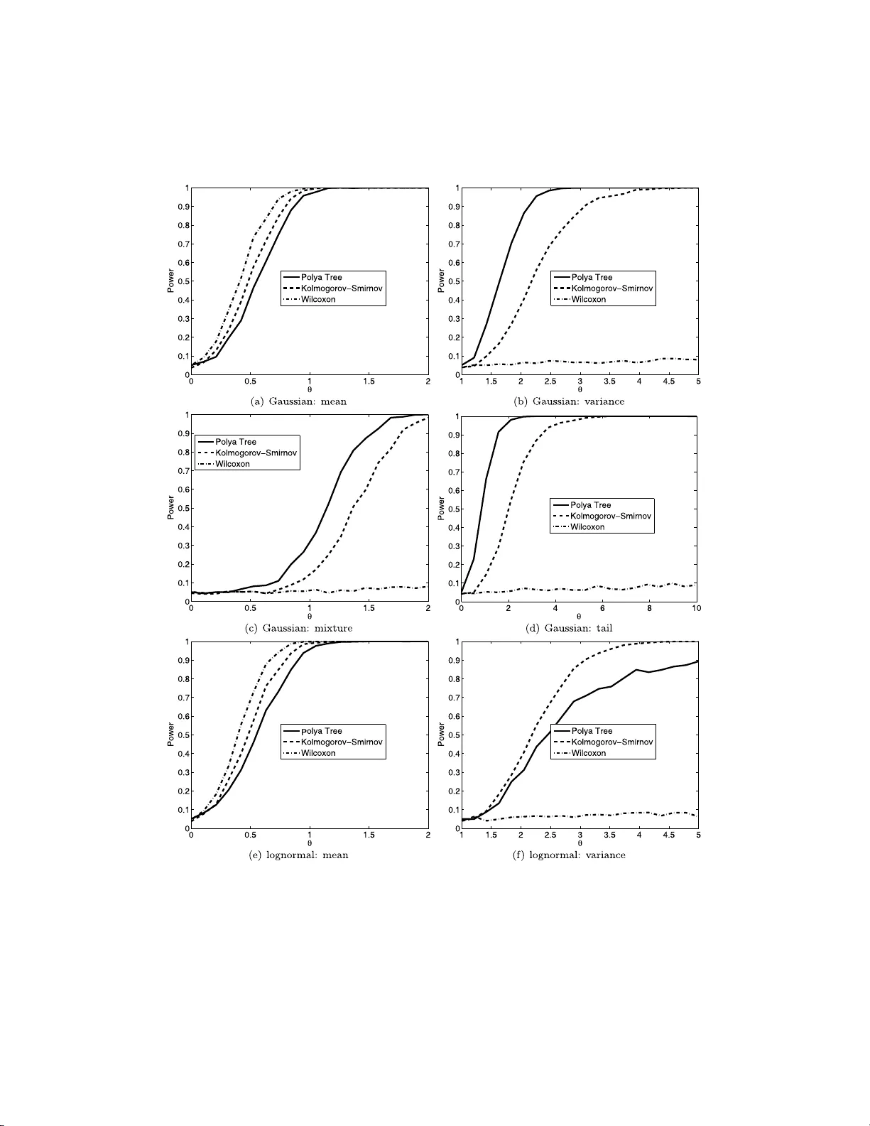
Ba yesi an Analysis (2015) 10 , Number 2, pp. 297–320 Tw o-samp le Ba y esian Nonpa rametric Hyp othesis T esting Chris C. Holmes ∗ , F ran¸ cois Caron † , Jim E. Griffin ‡ , and David A. Stephens § Abstract. In this article w e describe Bay esian nonparametric pro cedures for t w o- sample hypothesis testing. Namely , given tw o sets of samples y (1) iid ∼ F (1) and y (2) iid ∼ F (2) , with F (1) , F (2) unknown, w e wish to ev aluate the eviden ce fo r the null hypothesis H 0 : F (1) ≡ F (2) versus the alternative H 1 : F (1) 6 = F (2) . Our method is based up on a nonparametric P´ oly a tree prio r centered either sub jectively or using an empirical pro cedure. W e show that the P´ oly a tree prior leads to an analytic expression for the marginal likelihood under the tw o hypotheses and hence an explicit measure of th e probability of the null Pr( H 0 |{ y (1) , y (2) } ). Keyw ords: Bay esian n onparametrics , P´ o lya tree, hyp othesis testing. 1 Intro duction Nonparametric hypothesis tes ting is an imp ortant bra nch o f statistics with wide appli- cability . F or example we often wish to ev a lua te the evidence for s ystematic differences betw een real-v alued res ponses under tw o different tr e a tmen ts without sp ecifying an un- derlying distribution for the da ta. That is, given t wo sets of samples y (1) iid ∼ F (1) and y (2) iid ∼ F (2) , with F (1) , F (2) unknown, w e wish to e v a luate the evidence for the c ompeting hypotheses H 0 : F (1) ≡ F (2) versus H 1 : F (1) 6 = F (2) . In this article we des cribe a nonpar ametric Bayesian pro cedure for this scenario. Our Bay esian metho d quantifies the weigh t of evidence in fa vour of H 0 in terms of an ex- plicit pr obabilit y measure P r( H 0 | y (1 , 2) ), wher e y (1 , 2) denotes the p oo led data y (1 , 2) = { y (1) , y (2) } . T o p erform the test w e use a P´ olya tree prior (La vine, 1992 ; Mauldin et al., 1992 ; Lavine, 19 9 4 ) centered o n some distribution G where under H 0 we ha ve F (1 , 2) = F (1) = F (2) and under H 1 , F (1) 6 = F (2) are mo delled as indep enden t dr aws from the P´ olya tree pr ior. In this wa y we frame the test as a mo del compa r ison problem and ev alua te the Bayes F acto r for the tw o comp eting mo dels. The P´ o lya tree is a well known nonpar a metric prio r distribution for random pr obabilit y measures F o n Ω wher e Ω denotes the domain of Y (F erg uson, 1974 ). Bay esian nonpa rametrics is a fast developing discipline, but while ther e ha s b een considerable interest in nonpara metric inference there has somewhat sur prisingly b een ∗ Departmen t of Statistics and Oxford-Man Institute, Universit y of Oxford, England, c holmes@stats.o x.ac.uk † Departmen t of Statistics, Universit y of Oxford, England francois.caron@stats.o x.ac.uk ‡ Sc hool of Mathematics, Statistics and Actuarial Science, Unive rsity of K en t, England, J.E.Griffin-28@ken t.ac.uk § Departmen t of Mathematics and Statistics, McGil l Univ ersity , Canada, d.stephens@math.mcgill.ca c  2015 International Society for Ba yesian Analysis DOI: 10.1214 /14-BA914 298 Tw o-sample BNP Hyp othesis T esting little wr itten on nonparametric hypothes is testing. Bayesian par ametric h yp othesis test- ing w he r e F (1) and F (2) are of known for m is well develop ed in the B ayesian literature, see e.g. Bernar do a nd Smith ( 2000 ), and most nonpar ametric w ork has concentrated on testing a para metric mo del versus a nonparametr ic alternative (the Go o dness of Fit problem). Initial work on the Go o dnes s o f Fit problem (Florens et al., 1996 ; Ca r ota and Parmigiani, 1996 ) used a Diric hlet pro cess prior for the alternative distribution and compar ed to a pa r ametric mo del. In this case, the nonpar ametric distributions will be almost sure ly discre te, and the Bayes factor will include a penalty term for ties. The metho d ca n lead to misleading results if the da ta is absolutely co n tin uous, and has motiv ated the dev elopment of metho ds using nonparametric priors that gua r an tee almost surely con tinuous distributions. Dirichlet pr o cess mixture mo dels ar e one such class. The calculation of Bay es fa ctors for Dirichlet pr ocess- based mo dels is discussed by Basu and Chib ( 2003 ). Go o dness of fit testing using mixtures of tr iangular distr ibutio ns is considered by McVinish et a l. ( 2009 ). An alternative form o f prior, the P´ o ly a tree, was considered by Berger a nd Guglielmi ( 2001 ). Simple conditions on the prior lea d to absolutely contin uous distributions. Berger and Guglielmi ( 2001 ) develop a default ap- proach and consider its prop erties as a co nditional freque ntist metho d. Hans on ( 200 6 ) discusses the use of Sav a ge-Dic key density ra tios to calculate Bay es factor s in fav our of the cent ering distr ibution (see also B ranscum and Hanson ( 2008 )). Co nsistency is- sues are discussed by Da ss and Lee ( 2004 ), Ro usseau ( 2 007 ), Ghos al et al. ( 200 8 ) and McVinish et al. ( 200 9 ) . Ther e ha s b een s o me work on testing the h ypo thesis that tw o distributions are the same; Dunson and Peddada ( 2008 ) consider hypothesis tes ting of sto c hastic or de r ing using restricted Dirichlet pro cess mixtures, but their metho ds could be mo dified to allow tw o - sided hyp o theses. They consider a n in terv al null hypothesis and rely on Gibbs sampling for p osterior computation. Pennell and Dunson ( 2008 ) de- velop a Mix ture o f Dependent Dirichlet Pro cesses approach to testing changes in an ordered seque nce of distributio ns using a tolera nce mea sure. Bhattacharya and Dunson ( 2012 ) develop an a pproach for nonparametric Bay esian testing of differences b et ween groups, with the data within each group co nstrained to lie on a compact metric s pa ce or Riemannian manifold. Recently , following work presented here (or ig inally p osted on a rXiv in Holmes et a l. ( 2009 )), Ma and W ong ( 201 1 ) prop ose to allow the tw o random distributions under the alternative to randomly couple on different pa rts of the s a mple s pa ce, thereby achieving bo rrowing of information. Moreov er, Chen and Hans on ( 2014 ) prop ose to use Lavine’s (1992) partition fo r each F ( j ) centered at the normal distribution. Their approach en- ables generalization to more than tw o s amples, but contrary to our approach r e quires a truncation level to b e set. They also follow Ber ger and Guglielmi ( 2001 ) by cho osing the par ameter c that maximizes the Bayes factor in fav or o f the alterna tiv e. The r e st of the pa per is as follows. I n Section 2 we discus s the P´ olya tree prior and derive the marginal probability distributions that result from such a prior . In Section 3 we descr ibe our metho d and a lgorithm for calculating Pr( H 0 | y (1 , 2) ) ba sed on a sub- jective partitio n. In Section 4 we discuss an empiric al Bay es pro cedure where the P ´ oly a tree priors a re centered on the empirical cdf of the join t data. Se c tion 5 discusses the sensibility of the pro cedures to tuning parameter s. Sec tio n 6 provides a discussio n of related appr oac hes and Se c tion 7 concludes with a discussion o f p otential extensio ns. C. C. Ho lmes et al. 299 Figure 1: Co nstruction of a P´ olya tree distribution. E ac h of the θ ǫ m is indep enden tly drawn from Beta ( α ǫ m 0 , α ǫ m 1 ). Adapted from F er guson ( 1974 ). 2 P´ oly a tree p ri o rs P´ olya trees form a cla ss of distr ibutions for r andom probability mea sures F o n some domain Ω (Lavine, 1992 ; Mauldin et a l., 19 92 ; Lavine, 199 4 ). Consider a r ecursiv e dyadic (binary) partition of Ω into disjoint measurable sets. Deno te the k th level o f the partition { B ( k ) j , j = 0 , . . . , 2 k − 1 } , where B ( k ) i ∩ B ( k ) j = ∅ for all i 6 = j . The recur s iv e par titio n is constructed such that B ( k ) j ≡ B ( k +1) 2 j ∪ B ( k +1) 2 j +1 for k = 1 , 2 , . . . , j = 0 , . . . , 2 k − 1 . Figure 1 illustrates a bifurcating tr ee navigating the partition down to level three for Ω = [0 , 1). It will b e conv enient to index the partition elements using base 2 subscript and dro p the s uperscript so that, for example, B 000 indicates the first set in level 3, B 0011 the fourth set in level 4 a nd so on. T o define a rando m measure o n Ω we co nstruct random measures on the sets B j . It is instructive to imagine a particle cascading down through the tree such that at the j th junction the probability o f turning left or right is θ j and (1 − θ j ) resp ectively . In addition we conside r θ j to b e a random v ariable w ith some appro priate distr ibution θ j ∼ π j . The sample path o f the particle down to level k will b e r ecorded in a vector ǫ k = { ǫ k 1 , ǫ k 2 , . . . , ǫ kk } with elements ǫ ki ∈ { 0 , 1 } , such tha t ǫ ki = 0 if the particle wen t left a t level i , ǫ ki = 1 if it wen t right . Hence B ǫ k denotes which partition the particle belo ngs to at level k . By conv ention, set ǫ 0 = ∅ . Given a set of θ j s it is clear that the probability of the pa r ticle falling into the set B ǫ k is just P ( B ǫ k ) = k Y i =1 ( θ ǫ i − 1 ) (1 − ǫ ii ) (1 − θ ǫ i − 1 ) ǫ ii , which is just the pro duct of the probabilities of falling left or right a t ea c h junction tha t the par ticle pass e s thr o ugh. This defines a rando m measure o n the partitioning sets. Let Π denote the co lle c tion of sets { B 0 , B 1 , B 00 , . . . } a nd let A denote the collection of par ameters that determine the distribution at each junction, A = ( α 00 , α 01 , α 000 , . . . ). Definition 2.1. L avine ( 1992 ) A r andom pr ob ability m e asur e F on Ω is said to have a P´ olya tr e e distribution, or a P´ olya tr e e prior, with p ar ameters (Π , A ) , written F ∼ 300 Tw o-sample BNP Hyp othesis T esting P T (Π , A ) , if ther e exists nonne gative n umb ers A = ( α 0 , α 1 , α 00 , . . . ) and r andom vari- ables Θ = ( θ , θ 0 , θ 1 , θ 00 , . . . ) su ch that the fol lowing hold: 1. the ra ndom variables in Θ ar e mutu ally indep endent; 2. for every k = 1 , 2 , . . . and every ǫ k ∈ { 0 , 1 } k , θ ǫ k ∼ Beta ( α ǫ k 0 , α ǫ k 1 ); 3. for every k = 1 , 2 , . . . and every ǫ k ∈ { 0 , 1 } k , F ( B ǫ k | Θ) = k Y i =1 ( θ ǫ i − 1 ) (1 − ǫ ii ) (1 − θ ǫ i − 1 ) ǫ ii . (1) A rando m pr obabilit y meas ure F ∼ P T (Π , A ) is r ealized by sampling the θ j s from the Beta distributions. Θ is countably infinite as the tree extends indefinitely , and hence for most practical applica tions the tree is sp e c ified only to a depth m . Lavine ( 1994 ) refers to this as a “ partially s pecified” P´ olya tr ee. It is w orth noting that we will not need to make this truncation in what fo llows: o ur test will be fully sp ecified with analytic expressions for the ma rginal likeliho od. 1 By defining Π and A , the P´ olya tree ca n b e centered o n so me chosen distribution G so that E [ F ] = G where F ∼ P T (Π , A ). Perhaps the simplest way to a c hiev e this is to place the partitions in Π a t the quantiles of G a nd then set α ǫ k 0 = α ǫ j 1 for all k = 1 , 2 , . . . and all ǫ k ∈ { 0 , 1 } k . (Lavine, 1992 ). F o r Ω ≡ R this leads to B 0 = ( −∞ , G − 1 (0 . 5)), B 1 = [ G − 1 (0 . 5) , ∞ ) and, a t level k , B ǫ k = [ G − 1 { ( k ∗ − 1) / 2 k } , G − 1 ( k ∗ / 2 k )) , (2) where k ∗ is the decimal r epresen tation of the binary num ber ǫ k . It is usua l to set the α ’s to be constan t in a lev el α ǫ m 0 = α ǫ m 1 = c m for some constant c m . The se tting of c m gov erns the underlying contin uit y of the resulting F ’s. F or example, setting c m = cm 2 , c > 0, implies that F is absolutely contin uo us with probability 1 while c m = c/ 2 m defines a Dirichlet pro cess which makes F discrete with probability 1 (Lavine, 1992 ; F erguson, 1974 ). W e will follow the a pproac h o f W alker and Mallick ( 1999 ) and define c m = cm 2 . The choice of c is discussed in Section 5 . 2.1 Conditioning and ma rginal likeli ho o d An attractive featur e of the P´ olya tree prior is the ease with which we can condition on data. P ´ oly a trees exhibit conjugacy: given a P´ olya tree pr ior F ∼ P T (Π , A ) and data y drawn indep enden tly from F , then a p osteriori F also has a P´ olya tr e e distribution, F | y ∼ P T ( Π , A ∗ ) where A ∗ is the set of up dated para meters, A ∗ = { α ∗ 00 , α ∗ 01 , α ∗ 000 , . . . } α ∗ ǫ i | y = α ǫ i + n ǫ i , (3) 1 Note how ev er that consistency results only hold for a truncated version of the pr oposed test. C. C. Ho lmes et al. 301 where n ǫ i denotes the num b er of observ ations in y that lie in the par tition B ǫ i . The corres p onding ra ndom v ariables θ ∗ j are there fo re distr ibuted a p osteriori as θ ∗ j | y = Beta( α j 0 + n j 0 , α j 1 + n j 1 ) (4) where n j 0 and n j 1 are the num b ers of o bserv ations falling le ft a nd right at the junction in the tree indica ted by j . This conjuga c y allows for a straightforward ca lculation o f the marginal likelihoo d for any set o f o bserv ations, as Pr( y | Θ , Π , A ) = Y j θ n j 0 j (1 − θ j ) n j 1 (5) where θ j |A ∼ B e ( α j 0 , α j 1 ) and where the pro duct in ( 5 ) is over the set of all par ti- tions, j ∈ { 0 , 1 , 0 0 , . . . , } , thoug h clearly for many partitions we hav e n j 0 = n j 1 = 0. Equation ( 5 ) has the for m of a pro duct of indep enden t Bino mial-Beta trials hence the marginal likelihoo d is, Pr( y | Π , A ) = Y j  Γ( α j 0 + α j 1 ) Γ( α j 0 )Γ( α j 1 ) Γ( α j 0 + n j 0 )Γ( α j 1 + n j 1 ) Γ( α j 0 + n j 0 + α j 1 + n j 1 )  (6) where j ∈ { 0 , 1 , 0 0 , . . . , } . This marginal pro babilit y will form the ba sis of o ur test for H 0 which we descr ibe in the next section. 3 A p ro cedure fo r Bay esian nonpa rametric hyp othesis testing W e are int erested in providing a weight of evidence in favour of H 0 given the observed data. F rom Bay es theorem, Pr( H 0 | y (1 , 2) ) ∝ Pr( y (1 , 2) | H 0 )Pr( H 0 ) . (7) Under the n ull hypothesis H 0 , y (1) and y (2) are samples from some common distribu- tion F (1 , 2) with F (1 , 2) unknown. W e specify our uncertaint y in F (1 , 2) via a P´ olya tree prior, F (1 , 2) ∼ P T (Π , A ). Under H 1 , we assume y (1) ∼ F (1) , y (2) ∼ F (2) with F (1) , F (2) unknown. Again w e adopt a P´ olya tree prior for F (1) and F (2) with the same pr ior parameteriza tion a s for F (1 , 2) so that F (1) , F (2) , F (1 , 2) iid ∼ P T (Π , A ) (8) The logic for a dopting a common prior distr ibutio n is that we rega rd the F s as rando m draws from some universe of distributions that we descr ibe probabilis tica lly thro ugh the P´ olya tree distribution. Π is co nstructed from the quantiles of some a priori cen tering distribution. F ollowing the appr o ac h of W a lker and Mallick ( 1999 ); Mallick and W alker ( 2003 ) we tak e c o mmon v a lues for the α j s at e a c h level as α j 0 = α j 1 = c m 2 for an α parameter at level m . 302 Tw o-sample BNP Hyp othesis T esting The p osterior o dds on H 0 is Pr( H 0 | y (1 , 2) ) Pr( H 1 | y (1) , y (2) ) = Pr( y (1 , 2) | H 0 ) Pr( y (1) , y (2) | H 1 ) Pr( H 0 ) Pr( H 1 ) (9) where the first term is just the ratio of marginal likelihoo ds, the Bay es F a ctor, which from ( 6 ) a nd conditional on our sp ecification of Π and A , is P ( y (1 , 2) | H 0 ) P ( y (1) , y (2) | H 1 ) = Y j b j (10) where b j = Γ( α j 0 )Γ( α j 1 ) Γ( α j 0 + α j 1 ) Γ( α j 0 + n (1) j 0 + n (2) j 0 )Γ( α j 1 + n (1) j 1 + n (2) j 1 ) Γ( α j 0 + n (1) j 0 + n (2) j 0 + α j 1 + n (1) j 1 + n (2) j 1 ) × Γ( α j 0 + n (1) j 0 + α j 1 + n (1) j 1 ) Γ( α j 0 + n (1) j 0 )Γ( α j 1 + n (1) j 1 ) Γ( α j 0 + n (2) j 0 + α j 1 + n (2) j 1 ) Γ( α j 0 + n (2) j 0 )Γ( α j 1 + n (2) j 1 ) (11) and the pro duct in ( 10 ) is over a ll partitions, j ∈ {∅ , 0 , 1 , 0 0 , . . . , } , n (1) j 0 and n (1) j 1 represent the num b ers of o bs erv ations in y (1) falling rig h t and left at each junction and n (2) j 0 and n (2) j 1 are the equiv alent qua n tities for y (2) . W e can see from ( 10 ) that the ov erall Bay es F a ctor has the fo r m of a pro duct of Beta-Bino mial tests at each junction in the tree to b e interpreted a s “do es the data supp ort o ne θ j or tw o , { θ (1) j , θ (2) j } , in order to mo del the distribution of the observ ations going left and right at each junction?”, where for each j , θ j ∼ Beta( α j , α j ). The pro duct in ( 10 ) is defined ov er the infinite set of partitions. Howev er , for ea c h branch j , b j = 1 if n (1) j 0 + n (1) j 1 = 0 or n (2) j 0 + n (2) j 1 = 0; hence to calculate ( 10 ) for the infinite pa r tition structure we just have to m ultiply terms fro m junctions which contain at leas t some data from the tw o sets of samples . Hence, we only need sp ecify Π to the q uan tile le vel where partitions contain observ ations from b oth samples. Note a lso that in the complete absence of da ta (that is, when n (1) j 0 + n (2) j 0 = n (1) j 1 + n (2) j 1 = 0) b j = Γ( α j 0 )Γ( α j 1 ) Γ( α j 0 + α j 1 ) Γ( α j 0 )Γ( α j 1 ) Γ( α j 0 + α j 1 ) Γ( α j 0 + α j 1 ) Γ( α j 0 )Γ( α j 1 ) Γ( α j 0 + α j 1 ) Γ( α j 0 )Γ( α j 1 ) = 1 for all j , so the Bay es F actor is 1. The test pro cedure is des cribed in Algorithm 1 . 3.1 Prio r sp ecification The Bayesian pro cedure req uires the sp ecification o f { Π , A} in the P´ olya tree. While there are goo d guidelines for setting A the se tting of Π is more problem sp ecific, and the results will b e quite sensitive to this choice. O ur current, default, guideline is to first s ta ndardise the jo in t data y (1 , 2) with the median and interquant ile r ange of y (1 , 2) and then set the partition on the q uan tiles o f a standard no rmal dens it y , Π = Φ( · ) − 1 . C. C. Ho lmes et al. 303 Algorithm 1 Bayesian nonparametric test 1. Fix the bina ry tr ee on the quantiles of some centering distribution G . 2. F or level m = 1 , 2 , . . . , for ea ch j set α j = cm 2 for some c . 3. Add the log of the contributions of terms in ( 10 ) for each junction in the tree that has non-ze r o num bers of o bserv ations in y (1 , 2) going b oth right a nd left. 4. Rep ort Pr( H 0 | y (1 , 2) ) as Pr( H 0 | y (1 , 2) ) = 1 1+exp( − LO R ) , where LO R denotes the log o dd ratio calculated at step 3. W e ha ve found this to work well as a defa ult in most situations, though o f course the reader is e nc o uraged to set Π acco rding to their sub jectiv e b eliefs. In our algorithm, par a meter c is treated as a fixed hyper parameter. As we demo n- strate in Section 3.2 , a truncated version of our test with a sub jective partition is con- sistent under null and a lternativ e h ypo theses irr espective of the choice of c . Howev er , c does have an impact on finite sample prop erties, that is, the finite sample poster ior probabilities. This is alwa ys the case for Bay esian mo del selectio n/ h y pothesis testing based on the marginal lik eliho od, which is effectively a mea s ure of how well the prior predicts the obser v ed da ta, and no t a feature restricted to our nonpara metric pro cedure. In Section 5 w e provide some guidelines on the se nsitivit y of the testing pro cedure to the v alue of this par a meter, and discus s empirical Bay es estima tion of c . 3.2 Consistency Conditions for the consistency of the pro cedure under the null hypothesis and a lternativ e hypothesis ar e develop ed fo r a related test based on a truncation of the B ayes factor ( 9 ). Le t n = n (1) ∅ + n (2) ∅ be the total sample size for b oth sa mples . Let l ( ε ) b e the length of the vector ε . This also indicates tha t B ǫ forms par t of the partition a t level l ( ε ), and in our constructio n there are 2 l ( ǫ ) partition elements at level l ( ǫ ). W e consider the test statistics base d on the truncated Bay es factor B F κ 0 = Y { j | l ( j ) ≤ κ 0 } b j (12) where κ 0 ∈ N defines the level of truncation and can be set arbitra rily la rge. W e a ls o consider a tr uncated version of the hypothesis test: H 0 ,κ 0 : ∀ ǫ | l ( ǫ ) ≤ κ 0 , F (1) ( B ǫ ) = F (2) ( B ǫ ) versus H 1 ,κ 0 : ∃ ǫ | l ( ǫ ) ≤ κ 0 and F (1) ( B ǫ ) 6 = F (2) ( B ǫ ) . First, assume H 0 ,κ 0 is true and let F 0 denote the true distribution. T o pr o ve consis- tency under H 0 ,κ 0 , it is sufficient to show that lim n →∞ log B F κ 0 = ∞ as n → ∞ if b oth samples a r e drawn fr om the sa me distribution. 304 Tw o-sample BNP Hyp othesis T esting Theorem 3 . 1. Supp ose that t he limiting pr op ortion of observations in the first sample exists and is β ∅ : β ∅ = lim n →∞ n (1) ∅ n (1) ∅ + n (2) ∅ . (13) If 0 < β ∅ < 1 then, under H 0 ,κ 0 , lim n →∞ log B F κ 0 = ∞ and the t est define d by Algorithm 1 , trunc ate d at level κ 0 , is c onsistent under t he nul l. Pro of. See App endix. W e now co nsider co nsistency under H 1 ,κ 0 for the truncated version of the test. Theorem 3.2. Assume that 0 < β ∅ < 1 , and that ex ist s B ǫ , l ( ǫ ) ≤ κ 0 , such that F (1) ( B ǫ ) F (2) ( B ǫ ) > 0 and F (1) ( B ǫ 0 ) F (1) ( B ǫ ) 6 = F (2) ( B ǫ 0 ) F (2) ( B ǫ ) . Then lim n →∞ B F κ 0 = 0 and t he test define d by Algorithm 1 , tr u nc ate d at level κ 0 , is c onsistent u nder t he alter- native. Pro of. See App endix. The pro ofs for cons istency for the non-truncated test are muc h more challenging, as one needs to bo und terms at e a c h level of the P ´ oly a tr ee. In the next section, we provide nu merical exp erimen ts on the evolution of the Bayes factor with r espect to the sample size under b oth H 0 and H 1 , sug gesting consis tency for the non- truncated test. 3.3 Simulations T o examine the o p erating p erformance of the metho d we consider the following exp er- imen ts designed to e x plore v a rious canonical depar tures fro m the null. a) Mean s hift : Y (1) ∼ N (0 , 1), Y (2) ∼ N ( θ , 1), θ = 0 , . . . , 3. b) V ariance s hift : Y (1) ∼ N (0 , 1), Y (2) ∼ N (0 , θ 2 ), θ = 1 , . . . , 3. c) Mixtur e : Y (1) ∼ N (0 , 1 ), Y (2) ∼ 1 2 N ( θ , 1) + 1 2 N ( − θ , 1), θ = 0 , . . . , 3 . d) T ails: Y (1) ∼ N (0 , 1), Y (2) ∼ t ( θ − 1 ), θ = 10 − 3 , . . . , 10 whe r e t ( ν ) deno tes the standard Student t dis tribution with ν degrees of freedom. e) Lo gnormal mea n shift: log Y (1) ∼ N (0 , 1 ), lo g Y (2) ∼ N ( θ , 1), θ = 0 , . . . , 3. f ) Lognor ma l v aria nce shift: lo g Y (1) ∼ N (0 , 1 ), lo g Y (2) ∼ N (0 , θ 2 ), θ = 1 , . . . , 3. C. C. Ho lmes et al. 305 The default mean distr ibution F (1 , 2) 0 = N (0 , 1) was used in the P´ olya tree to constr uct the partitio n Π and α = m 2 . Data are standa rdized. Compa risons ar e pe rformed with n 0 = n 1 = 50 against the tw o-sample Kolmo gorov-Smirno v a nd Wilcoxon r ank test. T o compare the mo dels we explor e the “p o wer to detect the a lter nativ e”. As a test statis tic for the Bay esian mo del we simulate data under the null and then take the empirica l 0 . 95 q uan tile of the distribution of Bayes F actors as a threshold to decla re H 1 . This is known as “the Bay es, non-Bayes compro mise” by Go od ( 1992 ). Results, ba sed on 1000 replications, are re p orted in Figure 2 . As a g eneral rule we can see that the K S test is more sensitiv e to c hanges in cen tral loca tion while the Bay es test is mor e sensitive to changes to tails o r hig her mo men ts. The dyadic par titio n structure of the P´ olya T ree allows us to br eakdo wn the co n tr i- bution to the Bayes F actor by levels. That is, we can explore the contribution, in the log of equation (10 ), by level. This is shown in Fig ur e 3 as boxplots o f the distribution of log B F statis tics a cross the levels for the simulations genera ted for Figure 2 . This is a str e ngth of the P´ olya tree test in that it provides a q ua litativ e and quantitativ e decomp osition of the c o n tribution to the evidence aga inst the null from differing levels of the tr ee. It is also of interest to inv estigate the b ehavior of the Bay es factor a s a function of the sample size, b oth under the null and v a rious a lternativ es. Under the alternative, we consider in particular the following cases: a) Mean s hift : Y (1) ∼ N (0 , 1), Y (2) ∼ N (1 , 1). b) V ariance s hift : Y (1) ∼ N (0 , 1), Y (2) ∼ N (0 , 4). c) T ails: Y (1) ∼ N (0 , 1), Y (2) ∼ t (1). The r e sults ar e rep orted in Figure 4 fo r sample s ize n = 10 , 50 , 100 , 200 with 5 00 repli- cations, and seem to sug gest that the non-trunca ted test is consistent under the null and alterna tiv e. 4 A conditional p ro cedure The Bay esian proc edure abov e requires the sub jective specification of the partition structure Π. This sub jective setting ma y make some user s uneas y reg arding the sensi- tivit y to sp ecification. In this s ection we explore an empirical pro cedure whereby the partition Π is centered on the data v ia the empirical cdf of the joint data b Π = [ b F (1 , 2) ] − 1 . Let b Π b e the partition constructed with the q uan tiles of the empirical distr ibution b F (1 , 2) of y (1 , 2) . Under H 0 , there are now no fr ee par a meters and o nly one degre e of freedom in the rando m v a riables { n (1) j 0 , n (1) j 1 , n (2) j 0 , n (2) j 1 } a s conditiona l on the partition centered on the empirical cdf of the join t, once one of the v ar iables has been sp e cified the others are then known. W e consider, arbitr arily , the marg inal distribution of { n (1) j 0 } 306 Tw o-sample BNP Hyp othesis T esting Figure 2: P ow er o f Bay es test with α j = m 2 on s im ula tions fr om Section 3.3., with x-axis measur ing θ , the par ameter in the alternative. Legend: K-S (da shed), Wilcoxon (dot-dashed), Bayesian test (solid). C. C. Ho lmes et al. 307 Figure 3: Contribution to Bayes F actors from different levels of the P´ olya T ree under the alternative. Ga ussian distribution with v ar ying (a) mean (b) v arianc e (c) mixture (d) ta ils; log - normal distributio n with v arying (e) mean (f ) v ariance, from Section 3.2 . Parameters of H 1 were set to the mid-p oin ts of the x-a xis in Figure 2 . 308 Tw o-sample BNP Hyp othesis T esting Figure 4: Mean Bay es factor and 90% c onfidence int erv a l with r e spect to the s ample size n under (a) the null and (b-c) t wo Ga ussian distributions with different (b) means, (c) v a riances a nd (d) a Gaus sian a nd a Student t. which is no w a pro duct of hyperg eometric distributions (we only consider levels wher e n (1 , 2) j > 1) Pr( { n (1) j 0 }| H 0 , b Π , A ) ∝ Y j  n (1) j n (1) j 0   n (1 , 2) j − n (1) j n (1 , 2) j 0 − n (1) j 0    n (1 , 2) j n (1 , 2) j 0  (14) = Y j HG  n (1) j 0 ; n (1 , 2) j , n (1) j , n (1 , 2) j 0  (15) if max(0 , n (1 , 2) j 0 + n (1) j − n (1 , 2) j ) ≤ n (1) j 0 ≤ min( n (1) j , n (1 , 2) j 0 ), and zero o ther wise. Under H 1 , the ma r ginal distribution of { n (1) j 0 } is a pro duct of the conditiona l distri- C. C. Ho lmes et al. 309 bution of independent binomial v a riates, conditio nal on their s um, Pr   n (1) j 0    H 1 , b Π , A  ∝ Y j g  n (1) j 0 ; n (1 , 2) j , n (1) j , n (1 , 2) j 0 , θ (1) j , θ (2) j  P x g  x ; n (1 , 2) j , n (1) j , n (1 , 2) j 0 , θ (1) j , θ (2) j  (16) if max(0 , n (1 , 2) j 0 + n (1) j − n (1 , 2) j ) ≤ n (1) j ≤ min( n (1) j , n (1 , 2) j 0 ), zero otherwise , and wher e g  n (1) j 0 ; n (1 , 2) j , n (1) j , n (1 , 2) j 0 , θ (1) j , θ (2) j  = Bino mia l  n (1) j 0 ; n (1) j , θ (1) j  × . . . Binomial  n (1 , 2) j 0 − n (1) j 0 ; n (1 , 2) j − n (1) j , θ (2) j  and θ (1) j |A ∼ Beta( α j 0 , α j 1 ) θ (2) j |A ∼ Beta( α j 0 , α j 1 ) . Now, consider the o dds ra tio ω j = θ (1) j (1 − θ (2) j ) θ (2) j (1 − θ (1) j ) and let EHG  n (1) j 0 ; n (1 , 2) j , n (1) j , n (1 , 2) j 0 , ω j  = g ( n (1) j 0 ; n (1 , 2) j , n (1) j , n (1 , 2) j 0 , θ (1) j , θ (2) j ) P x g ( x ; n (1 , 2) j , n (1) j , n (1 , 2) j 0 , θ (1) j , θ (2) j ) . Then it can b een seen that EHG( x ; N , m, n, ω ) is the e x tended hypergeo metric distri- bution (Hark ness, 1965 ) whose p df is pro portional to HG( x ; N , m, n ) ω x , a ≤ x ≤ b, where a = max(0 , n + m − N ), b = min ( m, n ). Note there ar e C++ and R routines to ev aluate the p df. The ex tended hypergeo metric distr ibutio n mo dels a biased urn sampling scheme whereby there is a different likelihoo d of drawing one type of ball ov er another at each dr aw. The Bayes factor is now g iv en by B F = Y j HG  n (1) j 0 ; n (1 , 2) j , n (1) j , n (1 , 2) j 0  Z ∞ 0 EHG  n (1) j 0 ; n (1 , 2) j , n (1) j , n (1 , 2) j 0 , ω j  p ( ω j ) dω j (17) where the marg inal likelihoo d in the denominator can b e ev a luated us ing imp ortance sampling or o ne-dimensional quadratur e. The conditional Bay es tw o-sample test can then b e given in a s imilar way to Alg o - rithm 1 but now using ( 17 ) for the cont ribution at each junction. Conditio ns for the consistency o f the pro cedure under the null hypo thesis ar e develop ed fo r a rela ted test based on a truncation of the Ba yes factor ( 17 ) a lthough we hav e b een unable to show consistency under the a lternativ e. Theorem 4.1. Consider t he Bayes factor ( 17 ) tru nc ate d at level κ 0 B F κ 0 = Y j : l ( j ) ≤ κ 0 HG  n (1) j 0 ; n (1 , 2) j , n (1) j , n (1 , 2) j 0  Z ∞ 0 EHG  n (1) j 0 ; n (1 , 2) j , n (1) j , n (1 , 2) j 0 , ω j  p ( ω j ) dω j . (18) 310 Tw o-sample BNP Hyp othesis T esting Supp ose that β ∅ is as define d in Equation ( 13 ) . If 0 < β ∅ < 1 then, under H 0 ,κ 0 , lim n →∞ log B F κ 0 = ∞ and the t est is c onsistent un der the nu l l. Pro of. See App endix. W e repe ated the sim ulations from Section 3.3 with α = m 2 . The r esults ar e shown in Figure s 5 and 6 . W e observe similar b ehaviour to the test with sub jective par tition but impo rtan tly w e see that the problem in detecting the differ ence b et w een norma l and t- dis tribution is cor rected. Note that no sta ndardisation of the data is r equired for this test. 5 Sensitivit y to the pa rameter c The par ameter c acts as a precision para meter in the P ´ oly a tree and consequently can hav e a n effect o n the hypothesis testing pro cedures previously describ ed. In principle, the par ameter can b e chosen sub jectively as with pr ecision parameters in other mo dels (such as the linear mo del). Its effect is perhaps most easily under s too d through the prior v a riance of P ( B ǫ k ) which has the form (Hanson, 2006 ) V ar [ P ( B ǫ k )] = 4 − k   k Y j =1 2 cj 2 + 2 2 cj 2 + 1 − 1   . The pr ior v a riance tends to zero as c → ∞ and so the nonparametr ic prior places mass on distr ibutions which more closely r esem ble the cen tering dis tribution as c increases. Another consequence of this is that, under H 1 , c determines the a priori exp ected squared E uclidean distance be t ween F (1) ( B ǫ k ) a nd F (2) ( B ǫ k ), w he r e F (1) and F (2) are presumed indep enden tly drawn fro m P T (Π , A ); this distance diminishes as c increases : E [( F (1) ( B ǫ k ) − F (2) ( B ǫ k )) 2 ] = V ar h F (1) ( B ǫ k ) i + V ar h F (2) ( B ǫ k ) i = 4 − k + 1 2   k Y j =1 2 cj 2 + 2 2 cj 2 + 1 − 1   . The v alue of c can be chosen to co n trol the ra te at which the v ar iances decreas es. W e hav e found v a lues o f c be tw een 1 and 10 work well in pra ctice. Fig ures 7 and 8 show results for different v alues of c . As with a n y B a y esian testing pro cedure, we recommend chec k ing the sensitivity of their results to the chosen v alue o f the hyperpa r ameter c . An alterna tiv e approach to the c hoice of c in hypo thesis testing is g iven by Ber ger and Guglielmi ( 2001 ) in the context of testing a pa rametric mo del a gainst a nonpara- metric a lternativ e. They argue that the minim um of the Bay es factor in fav our of the parametric mo del is useful since the parametric mo del ca n be considered s a tisfactory C. C. Ho lmes et al. 311 Figure 5: As in Figure 2 but now using conditiona l Bayes T est with α j = m 2 . 312 Tw o-sample BNP Hyp othesis T esting Figure 6: Contribution to the Bay es F a ctor for different levels o f the conditiona l P ´ oly a tree prior for Gaussian distribution with v arying (a) mea n (b) v a riance (c) mixture (d) tails; log- normal distribution with v arying (e) mean (f ) v ar ia nce. C. C. Ho lmes et al. 313 Figure 7: Sub jective test with empirical Bay es estimation of the para meter c for (a) mean shift (b) v a r iance shift. Point estimates of c are o btained by max imizing b oth the ma rginal likelihoo d under the null and alterna tiv e ov er the grid of v alues 10 i for i = − 2 , − 1 , . . . , 3. if the “ minim um is not to o s ma ll”. It is the Bay es factor calculated using the empir - ical Bayes (Type I I maximum likelihoo d) estimate of c . W e sug g est ta king a similar approach if c cannot b e sub jectively chosen. In the test with s ub jectiv e partition, the empirical Bayes estimates ˆ c ar e calculated under H 0 and under H 1 . Using these v alues, the Bay es fa ctor ca n b e interpreted as a likelihoo d ratio statistic for the compar ison of the t wo hypo thes es. In the co nditional test, the empir ical Bayes estima te is calculated only under H 1 (since the marginal likeliho od under H 0 do es not depe nd on c ). Figures 7 and 8 provide results for mean and v a riance shifts with c estima ted ov er a fixed g rid using this pro cedure. W e also p erformed exp eriments to test the sensitivity of the pro cedure to the parti- tion. Exp eriment s (not rep orted her e) with a partition centered on a standar d Studen t t distribution show e d little difference co mpared to a partition centered on a s tandard Gaussian distribution. 6 Discussion and rela ted w o r k There hav e b een several other a pproaches to testing the difference betw een tw o distri- butions using P´ olya tr ee based a pproach es. Ma and W o ng ( 2011 ) pro pose the Coupling Optional P´ o ly a tree (co- opt) pr ior which ex tends their previous work on O ptional P´ olya tree prior s (W ong and Ma, 2010 ). The Optional P ´ oly a tree defines a pr ior for a single distribution. A prio r is defined on the sequence of partitions used to construct the P´ olya tree. This allows the partition to b e c o ncen trated on are a s of the sample space whic h hav e the larg est difference from the base meas ure (which is the unifor m in their c ase). The co-o pt prior is suitable for t wo distributions with a partition defined for each distri- bution. The prior allows coupling of tw o partitions so that if a set A (which is member 314 Tw o-sample BNP Hyp othesis T esting Figure 8: Conditional test with empirica l Bayes e stimation of the parameter c for (a) mean shift (b) v a riance shift. Poin t estimate of c is obtained by maximizing the mar ginal likelihoo d under the a lternativ e ov er the grid of v alues 10 i for i = − 2 , − 1 , . . . , 3 . of the partition at level m ) is coupled then all subsequent partitions of A will b e the same for the t wo dis tr ibutions. This allows the p osterior to concentrate these co uplings on parts of the supp ort of the tw o distributions where they are similar and so allows the b orrowing of s trength b etw een the tw o distributions. The pr ior is conjugate and can b e used to b oth test for differences b e tw een tw o distributions and to infer where these differences o ccur in the p osterior. The prior is particula rly suited to multiv ariate problems due to its ability to efficiently learn the partitio n of the da ta. The p o sterior is av ailable in closed form but ca n b e computationally exp ensive to calculate in practice with computatio na l time scaling exp onent ially with sample size. Chen and Hanson ( 20 14 ) pro pose a metho d for comparing k -samples of data which may b e ce nsored. They test the null hypothesis tha t the distribution of ea c h sample is the same ag ainst the alter nativ e that the samples ar ise from at lea st tw o different distri- butions. Under the null hypothesis, the common distribution is given a P´ olya tree prio r whereas, under the alter na tiv e h yp othesis, each distribution is given an indep enden t P´ olya tree prior. All P´ olya tree priors are centered ov er a nor mal distribution whose parameters are estimated using maxim um likeliho od to define an empir ical Bay es pro- cedure. Different pa rtitions are use d for the P´ olya tree distr ibutions under the null and the alternative hypo thes e s and so the par tition must b e truncated in o rder to compute the Bayes facto r, co n tr a ry to o ur simpler approa c h which inv olves no truncatio n. 7 Conclusions W e hav e describ ed a Bay esian nonpar ametric hypo thesis test for real v alued data which provides an explicit measure of Pr( H 0 | y (1 , 2) ). The test is based o n a fully sp ecified P ´ oly a tree prior fo r which we a re a ble to der iv e an explicit form for the Bay es F actor. C. C. Ho lmes et al. 315 Conditioning on a particular partition ca n lead to a predictive distribution that exhibits jumps at the pa rtition b oundary p oin ts. This is a well-known phenomeno n of P´ olya tree priors and some interesting directions to mitigate its effects can b e found in Hanson and Johnso n ( 2002 ); Paddo c k e t al. ( 2003 ); Hanson ( 2006 ). W e do not cons ider these appr oac hes here as mixing ov er partitions w ould lo se the analytic tra ctabilit y o f our appr o ac h, but it is an interesting area for future study and is considered by Chen and Hanson ( 2014 ). Ackno wledgem ents This research was pa rtly supp orted by the Oxford-Ma n Institute (OMI) thro ugh a visit by FC to the OMI. F C thanks P ie rre Del Moral for helpful discussio ns on the pro ofs of cons is tency a nd ackno wledges the supp ort of the E uropean Co mmission under the Marie Cur ie Intra-Europ ean F ellowship P rogramme. DS ackno wledges the supp ort of a Discov ery Grant from the Natura l Sciences and Eng ineering Council of Canada. The authors thank reviewers of earlier versions of this ar ticle for helpful comments. References Basu, S. and Chib, S. (2 003). “Mar g inal likeliho od and Ba yes facto r s for Dirichlet pro cess mixture mo dels.” Journal of the Ameri c an St atistic al Asso ciation , 98: 2 2 4– 235. 298 Berger, J. O. and Guglielmi, A. (2001). “ T esting of a pa r ametric mo del versus nonpar a - metric a lter nativ es.” Journal of the Americ an St atist ic al Asso ciation , 96: 174 –184. 298 , 310 Bernardo , J. M. and Smith, A. F. M. (20 00). Bayesi an the ory . Chichester: John Wiley . 298 Bhattacharya, A. and Dunson, D. B . (2012). “Nonpa rametric Bay es Classification and Hypo thesis T esting on Manifolds.” Jour n al of mu ltiva riate analysis , 11 1: 1–1 9 . 298 Branscum, A. J. and Hanson, T. J. (200 8 ). “Bay esian nonpa rametric meta-analy sis using Polya tr ee mixture mo dels.” Biometrics , 64: 8 25–833. 298 Carota, C. a nd P armigia ni, G. (19 96). “ O n Bayes F actors for Nonpara metric Alterna - tives.” In Ber nardo, J. M., Ber ger, J. O ., Dawid, A. P ., a nd Smith, A. F. M. (eds.), Bayesian Statistics 5 , 508 –511. London: Oxford Universit y Pr ess. 298 Chen, Y. and Hanson, T. E. (2014). “ Ba yesian nonparametr ic k-sa mple tes ts for cen- sored and uncensored data.” Computational S tatistics & Data Analysis , 7 1: 335–3 40. 298 , 314 , 3 15 Dass, S. C. and Lee, J. (2 0 04). “A note on the consistency of Bayes factors for tes ting po in t null v ersus non-par ametric alter nativ es.” Journal of Statist i c al Planning and Infer enc e , 11 9: 143– 152. 29 8 Dunson, D. B. and Peddada, S. D. (2008 ). “Bay esian nonpara metric inference on sto c hastic o rdering.” Biometrika , 95: 859 –874. 298 316 Tw o-sample BNP Hyp othesis T esting F erg uson, T. S. (1974). “Prior distributions on spa c e s o f pro babilit y measures.” The Annals of St atistics , 2: 61 5–629. 297 , 29 9 , 300 Florens, J. P ., Richard, J. F., and Rolin, J. M. (19 96). “ B a y esian Encompass ing Specifi- cation T ests o f a Parametric Mo del Against a Nonpar ametric Alter na tiv e.” T echnical Repo rt 96 .08, Institut de Statistique, Universit´ e Catholique de Lo uv a in. 298 Ghosal, S., Lember, J., and V an der V aa rt, A. (200 8). “ Nonparametric Bay esian mo del selection and av eraging.” Ele ctr onic J ournal of Statistics , 2: 63–8 9. 298 Go od, I. J. (1992 ). “The B ayes/non-Bay es compromise: a brief review.” Journ al of t he Americ an Statistic al Asso ciation , 87: 597 –606. 305 Hanson, T. E . (2006 ). “ Inference for mixtures o f finite P oly a tree mo dels.” Journal of the Americ an Statistic al Asso ciation , 10 1: 154 8–1565. 298 , 3 10 , 3 1 5 Hanson, T. E. and J ohnson, W. O. (20 02). “ Modeling re gression error with a mixture of Polya trees.” Journal of t he Americ an Statistic al Asso ciatio n , 9 7: 10 20–1033. 315 Harkness, W. L. (1965 ). “Pr operties of the extended hyper geometric distribution.” The Annals of Mathematic al Statist ics , 36 : 938–9 45. 309 , 320 Holmes, C. C., Ca ron, F., Gr iffin, J. E ., and Stephens, D. A. (2009 ). “Two-sample Bay esian nonparametr ic hypo thesis testing.” T echnical r eport, arXiv: 0910.5 060 [stat.ME]. 298 Kass, R. a nd Ra ft ery , A. (199 5). “Bayes factor s.” Journal of the Americ an Statistic al Asso ciation , 90: 7 73–795. 320 Lavine, M. (199 2). “Some asp ects of Polya tree distributions for statistical mo delling.” The Annals of Statistics , 20: 12 2 2–1235. 297 , 299 , 3 00 — (1994 ). “More asp ects o f Po ly a tree distr ibutions for statistical mo delling.” Th e Annals of St atistics , 22: 1 161–1176 . 297 , 299 , 300 Ma, L. and W o ng , W. H. (2011). “Co upling optional P´ olya trees and the tw o sample problem.” Journal of the Americ an Statistic al Asso ciation , 1 06(496): 1553– 1565. 298 , 313 Mallick, B. K. and W alker, S. G. (2003). “A Bay es ian semiparametr ic transfo rmation mo del incorp orating fra ilties.” Journal of S t atistic al Planning and Infer enc e , 1 12: 159–1 74. 301 Mauldin, R. D., Sudder th, W. D., and Williams, S. C. (19 92). “ Poly a trees and random distributions.” The Annals of Statist ic s , 20: 1 2 03–1221. 297 , 299 McVinish, R., Ro usseau, J., and Mengerse n, K . (2009). “Bayesian Go odnes s of Fit T est- ing with Mixtures of T ria ngular Distributions.” Sc andinavian Journal of St atistics , 36: 337– 354. 298 Paddock, S. M., Rugg eri, F., Lavine, M., a nd W est, M. (2003 ). “ Randomized P oly a tree mo dels for nonpara metric Bay esian inference.” Statistic a Sinic a , 13: 44 3–460. 315 C. C. Ho lmes et al. 317 Pennell, M. L. and Dunso n, D. B. (20 08). “No npa rametric Bayes T esting of Changes in a Resp onse Distribution with an Ordinal P redictor.” Biometrics , 64: 413–4 23. 298 Rousseau, J. (2007). “Approximating Interv al hypothesis : p-v alues a nd Bay es factor s.” In Berna rdo, J. M., Berger , J. O ., Dawid, A. P ., and Smith, A. F. M. (eds.), Bayesian Statistics 8 . Oxfor d Universit y Press . 298 W alker, S. G. and Mallick, B. K . (1999). “A Bay esian semiparametric a ccelerated failure time mo del.” Biometrics , 55 : 477 –483. 300 , 30 1 Wilks, S. (1938 ). “The large- sample distribution o f the lik eliho od r atio for tes ting comp osite hypo theses.” The Annals of Mathematic al St atistics , 9 : 60– 62. 3 18 , 320 W ong, W. H. and Ma, L. (2010 ). “Optiona l P oly a tre e and Bay esian inference.” The Annals of St atistics , 38(3): 1 433–1459 . 3 13 App endix: Pro ofs Pro of of Theorem 1 Clearly the log Bayes factor is log B F κ 0 = X { j | l ( j ) ≤ κ 0 } log b ( n ) j . Stirling’s appr o ximation o f the Gamma function allows us to write b ( n ) j ≃ Γ( α j 0 )Γ( α j 1 ) Γ( α j 0 + α j 1 ) 1 √ 2 π  b p (1 , 2) j 0  α j 0 − 1 / 2  b p (1 , 2) j 1  α j 1 − 1 / 2  b p (1) j 0  α j 0 − 1 / 2  b p (1) j 1  α j 1 − 1 / 2  b p (2) j 0  α j 0 − 1 / 2  b p (2) j 1  α j 1 − 1 / 2 × s n (1) j n (2) j n (1 , 2) j ×  b p (1 , 2) j 0  n (1 , 2) j 0  b p (1 , 2) j 1  n (1 , 2) j 1  b p (1) j 0  n (1) j 0  b p (1) j 1  n (1) j 1  b p (2) j 0  n (2) j 0  b p (2) j 1  n (2) j 1 (19) where b p ( k ) j 0 = n ( k ) j 0 n ( k ) j 0 + n ( k ) j 1 b p ( k ) j 1 = 1 − b p ( k ) j 0 . W e hav e, under the null, s n (1) j n (2) j n (1 , 2) j ≃ √ n q F 0 ( B j ) β ∅ (1 − β ∅ ) . (20) The term L j =  b p (1 , 2) j 0  n (1 , 2) j 0  b p (1 , 2) j 1  n (1 , 2) j 1  b p (1) j 0  n (1) j 0  b p (1) j 1  n (1) j 1  b p (2) j 0  n (2) j 0  b p (2) j 1  n (2) j 1 (21) 318 Tw o-sample BNP Hyp othesis T esting is a likeliho od ra tio for testing comp osite h yp otheses H j 0 : p (1) j 0 = p (2) j 0 = p (1 , 2) j 0 vs H j 1 :  p (1) j 0 , p (2) j 0  ∈ [0 , 1 ] 2 with n (1) j 0 ∼ Bino mial  n (1) j , p (1) j 0  and n (2) j 0 ∼ Binomial  n (2) j , p (2) j 0  . Clearly b p (1 , 2) j 0 and  b p (1) j 0 , b p (2) j 0  are the maximum likelihoo d estimators under H j 0 and H j 1 resp ectiv ely . It follows tha t, under H j 0 , − 2 log L j asymptotically follows a χ 2 distribution (Wilks, 1938 ). Finally , if β ∅ (1 − β ∅ ) > 0 a nd using Equation ( 20 ), then Theorem 1 follows. Pro of of Theorem 2 If F (1) ( B j ) = 0 or F (2) ( B j ) = 0, then we have trivially lo g( b j ) = 0. W e as sume that F (1) ( B j ) F (2) ( B j ) > 0 (22) 0 < β ∅ < 1 . (23) If p (1) j 0 = p (2) j 0 then, from the previous section, log( b j ) go es to ∞ in o (log( n )). W e consider now the case p (1) j 0 6 = p (2) j 0 . Let b β ( n ) j = n (1) j /n (1 , 2) j , β j = lim n →∞ b β ( n ) j = β ∅ F (1) ( B j ) F (1 , 2) ( B j ) with F (1 , 2) ( B j ) = β ∅ F (1) ( B j ) + (1 − β ∅ ) F (2) ( B j ). Under assumptions ( 22 ) and ( 23 ), we hav e 0 < β j < 1. Let L j be defined as in Equa tion ( 21 ). W e hav e log L j = η j − n (1 , 2) j ζ j where η j = n (1 , 2) j H p (1 , 2) j 0  b p (1 , 2) j 0  − n (1) j H p (1) j 0  b p (1) j 0  − n (2) j H p (2) j 0  b p (2) j 0  , ζ j = b β ( n ) j H 1  p (1) j 0  +  1 − b β ( n ) j  H 1  p (2) j 0  − H 1  p (1 , 2) j 0  , p ( k ) j 0 = lim n →∞ b p ( k ) j 0 , k = 1 , 2 , { 1 , 2 } and the function H p : x ∈ (0 , 1) → R + is defined for p ∈ (0 , 1 ) by H p ( x ) = x log  x p  + (1 − x ) lo g  1 − x 1 − p  . Consider first the ter m ζ j . W e have p (1 , 2) j 0 = β j p (1) j 0 + (1 − β j ) p (2) j 0 and n − → ∞ , therefo r e ζ j − → β j H 1  p (1) j 0  + (1 − β j ) H 1  p (2) j 0  − H 1  p (1 , 2) j 0  . C. C. Ho lmes et al. 319 As the function H p is conv ex, it follows that ζ j tends to a p ositiv e consta n t if p (1) j 0 6 = p (2) j 0 . Hence n (1 , 2) j ζ j tends to ∞ in o ( n ). Consider now η j which is approximately equal to Y j = n (1 , 2) j 2 p (1 , 2) j 0  1 − p (1 , 2) j 0   b p (1 , 2) j 0 − p (1 , 2) j 0  2 − n (1) j 2 p (1) j 0  1 − p (1) j 0   b p (1) j 0 − p (1) j 0  2 − n (2) j 2 p (2) j 0  1 − p (2) j 0   b p (2) j 0 − p (2) j 0  2 . Then Y j = − n (1 , 2) j b β ( n ) j  1 − b β ( n ) j  2 p (1 , 2) j 0  1 − p (1 , 2) j 0   b p (1) j 0 − b p (2) j 0 −  p (1) j 0 − p (2) j 0  2 + n (1 , 2) j b β ( n ) j  1 − ρ (1) j  2 p (1 , 2) j 0  1 − p (1 , 2) j 0   b p (1) j 0 − p (1) j 0  2 + n (1 , 2) j  1 − b β ( n ) j   1 − ρ (2) j  2 p (1 , 2) j 0  1 − p (1 , 2) j 0   b p (2) j 0 − p (2) j 0  2 where ρ ( k ) j = p (1 , 2) j 0  1 − p (1 , 2) j 0  p ( k ) j 0  1 − p ( k ) j 0  . W e hav e a s ymptotically Y j ≃ nF (1 , 2) ( B j ) − β j (1 − β j ) 2 p (1 , 2) j 0  1 − p (1 , 2) j 0   b p (1) j 0 − b p (2) j 0 −  p (1) j 0 − p (2) j 0  2 + β j  1 − ρ (1) j  2 p (1 , 2) j 0  1 − p (1 , 2) j 0   b p (1) j 0 − p (1) j 0  2 + (1 − β j )  1 − ρ (2) j  2 p (1 , 2) j 0  1 − p (1 , 2) j 0   b p (2) j 0 − p (2) j 0  2 ! . W e hav e a quadratic form Y j ≃ − nF (1 , 2) ( B j ) β j (1 − β j ) 2 p (1 , 2) j 0  1 − p (1 , 2) j 0    b p (1) j 0 − p (1) j 0   b p (2) j 0 − p (2) j 0   A   b p (1) j 0 − p (1) j 0   b p (2) j 0 − p (2) j 0   with squa re matrix A =     ρ (1) j − β j 1 − β j − 1 − 1 ρ (2) j − 1 + β j β j     and so a symptotically √ n   b p (1) j 0 − p (1) j 0   b p (2) j 0 − p (2) j 0   ∼ N     0 2 ,     p (1) j 0  1 − p (1) j 0  β j F (1 , 2) ( B j ) 0 0 p (2) j 0  1 − p (2) j 0  (1 − β j ) F (1 , 2) ( B j )         320 Tw o-sample BNP Hyp othesis T esting which is independent of the sample s ize, and it follows that Y j asymptotically follows a sc aled χ 2 distribution and log L j go es to −∞ in o ( n ). T o conclude, w e have that in Equation ( 19 ) s n (1) j n (2) j n (1 , 2) j ≃ √ n q F (1 , 2) ( B j ) β j (1 − β j ) . It follows that • If F (1) ( B j ) F (2) ( B j ) = 0, log( b j ) = 0. • If F (1) ( B j ) F (2) ( B j ) > 0 – If p (1) j 0 6 = p (2) j 0 , the log-co n tribution log ( b j ) go es to − ∞ at a r ate of o ( n ). – If p (1) j 0 = p (2) j 0 , the log-co n tribution log ( b j ) go es to + ∞ at a r ate of o (log n ). Pro of of Theorem 3 The co ndition β ∅ (1 − β ∅ ) implies tha t β j (1 − β j ) > 0 for all j . Let b ( n ) j = HG  n (1) j 0 ; n (1 , 2) j , n (1) j , n (1 , 2) j 0  Z ∞ 0 exp { u ( ω j ) } dω j (24) where u ( ω j ) = log EHG  n (1) j 0 ; n (1 , 2) j , n (1) j , n (1 , 2) j 0 , ω j  + log p ( ω j ). Then log B F κ 0 = X { j | l ( j ) ≤ κ 0 } log b ( n ) j . Under the conditions β j (1 − β j ) > 0 , the max im um likeliho od estimate b ω j of the pa- rameter ω j in the ex tended h yp ergeometric distr ibution conv erges in probability to the true par ameter (Harkness, 1965 , p. 944 ). W e can there fore use a Laplace appr o xima- tion (Kass and Raftery, 1995 ) of the deno minator in ( 24 ), we obtain for n (1) j 0 large b ( n ) j ≃ HG  n (1) j 0 ; n (1 , 2) j , n (1) j , n (1 , 2) j 0  √ 2 π | b Σ j | 1 / 2 EHG  n (1) j 0 ; n (1 , 2) j , n (1) j , n (1 , 2) j 0 , b ω j  p ( b ω j ) where b ω j = argmax ω j u ( ω j ) and b Σ − 1 j = − D 2 u j ( b ω j ), where D 2 u j ( b ω j ) is the Hessian matrix of s econd der iv ativ es. The r atio r j = HG  n (1) j 0 ; n (1 , 2) j , n (1) j , n (1 , 2) j 0  EHG  n (1) j 0 ; n (1 , 2) j , n (1) j , n (1 , 2) j 0 , b ω j  = EHG  n (1) j 0 ; n (1 , 2) j , n (1) j , n (1 , 2) j 0 , 1  EHG  n (1) j 0 ; n (1 , 2) j , n (1) j , n (1 , 2) j 0 , b ω j  is a likeliho od ra tio for testing the co mposite hypothese s H j 0 : ω j = 1 vs H j 1 : ω j > 0 , hence − 2 log r j is asymptotically χ 2 -distributed (Wilks, 1938 ). And as | b Σ j | → 0 as n → ∞ , then b ( n ) j → ∞ for all j as n → ∞ .