A Level Set Approach to Online Sensing and Trajectory Optimization with Time Delays

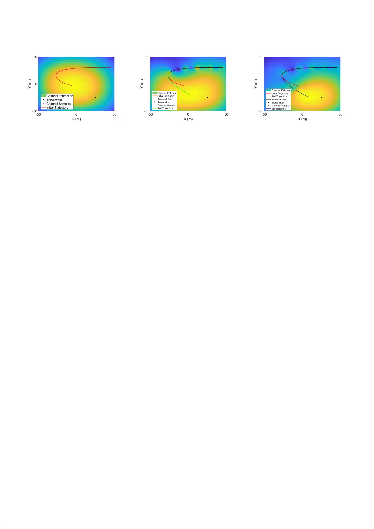
A Lev el Set App roac h to Online Sensing and T ra jectory Optimizatio n with Time Dela ys ⋆ Matthew R. Kirc hner ∗ , ∗∗ ∗ Image and Signal Pr o c essing Br anch, R ese ar ch Dir e ctor ate, Naval Ai r W arfa r e Center W e ap ons Division, China L ake, CA 93555, U SA (e-mail: matthew.kir chner@navy.mil) ∗∗ Ele ctric al and Computer Engine ering Dep artment, University of Califo rnia, Santa Barb ar a, CA 93106, USA (e-mail: kir chner@ucsb.e du) Abstract: Presented is a metho d to compute certain classes of Hamilton–J acobi equations that result fro m optimal control and tra jectory generation problems with time delays. Many rob otic control and tra jecto r y problems ha ve limited information of the oper ating en vironment a priori and m ust contin ua lly perform online tra jectory optimization in real time after collecting measurements. The sensing a nd o ptimization can induce a s ignificant time delay , a nd must be accounted for when co mputing the tra jectory . This paper utilizes the ge ner alized Hopf formula, which av o ids the exp onential dimensional s caling typical of other numerical metho ds for computing solutions to the Hamilton–Jacobi equation. W e present as an example a rob ot that incrementally predicts a communication channel from measurements as it travels. As par t of this example, we int ro duce a seeming ly new generaliza tion of a non-para metric formulation of rob otic communication channel estimation. New communication measurements ar e use d to improv e the c hannel estimate and online tra jectory optimization with time-delay compensation is p erformed. Keywor ds: Time Delay Systems, Hamilton–Jacobi Equation, Genera lized Hopf F ormula, Viscosity Solution, Optimal Co ntrol, Communi cation Seeking Rob otics 1. INTRODUCTION Time delays ar e common presence in re a l-world instan tia - tions of dyna mic systems. This causes issues with stability and robustness when attempting to design real-time con- trol for these systems, and the challenges of desig n and analysis of systems with time delays hav e b een well stud- ied; see Richard (2003 ). Historica lly , ther e hav e b een many attempts to comp ensate for time delays in co nt rol theory , such as the well-known P adé approximation in class ical linear control theory (F ranklin et a l., 20 06, Sec. 5.7.3), which approximates a pure delay as a ra tional transfer function or state transformatio ns s uch as presented in Kw o n a nd Pearson (1 980). In a mo dern setting, r eal-time optimal control (R TOC) [Ro ss et al. (2006 )] and mo del predictive control (MPC) [Ca macho and Alba (2013)] have gained large sca le acce pta nce in control and tra jectory op- timization problems. These seek to find a control sequence and the resulting tra jector y that minimizes a pre-defined cost functional. R TOC optimizes the co st functional di- rectly , while MPC computes o n a finite time horizon and is frequently referred to a s receding ho r izon con trol. Becaus e of this, MPC is sub-o ptimal and necessitates online re- computation of the current state frequently , while R TO C only needs to b e re- computed o nline if the system is p er- turbe d from the computed optimal tra jectory . ⋆ This researc h w as supported by the Office of Na v al Researc h under Gran t N00014-18-WX01382. F ast online co mputation is critica l for these a pproaches, and delay from computation b ecomes more appa r ent as the dimensionality and mo del complexity of the optimization increases. In addition to time dela ys induced from compu- tation, many r ob otics pro blems hav e limited information of the o pe r ating en vironment a prio ri. The rob ot must per form sensing in real- time and a s a result, necessitates online re-compuatio n of the optimal tra jectory with this new information. As metho ds for sensing in r ob otics hav e bec o me mo r e s ophisticated, the time delay induced be- comes large r. An illustrative exa mple app ear e d in Usman et al. (201 6), where a complicated non-pa rametric mo del was used to estimate the qua lit y of a communication signal from measurements of a transmitter with a known lo cation. In that work, a R TOC s cheme was developed to minimize combined motion and communication e ner gy of the sig nal. The R TOC was re-computed every 10 seconds and it w as noted th at the com bined sensing and tra jectory optimization was around 2 seco nds, or 20% of the entire compute interv a l. A delay this large ca n hav e drastic con- sequences if not acco unted for . This was not addr e ssed in Usman et al. (201 6 ). As noted in Lu (2008 ), attempts to directly acco unt for time delays in MPC formulations are limited, with the most notable pr op osed in Kwon et al. (2 004) for linea r systems. How ever this work is restricted to a specific LQR cost functional and do es not acco unt for control satura tion. W e pres ent in this pap er a more g eneral approa ch based on Hamilton– J acobi theory , which provides a natura l way to deal with pure time delay in the control. Generally , solutions to optimal co ntrol and tra jectory problems ca n be found by solving a Hamilton–Jac o bi (HJ) partial different ial equation (PDE) as it establishes a sufficient co ndition for o ptimalit y [Osmolovskii (19 9 8)]. T raditionally , n umerical solutions to HJ equations r equire a dense, discrete grid of the so lution space as in Osher a nd F edkiw (20 06); Mitchell (2008 ). Computing the elements of this grid sca les p o or ly with dimension and has limited use for problems with dimension gr eater than four. The exp onential dimensional scaling in optimization is some- times referred to a s the “curs e of dimensionality” [Bellman (1957)]. A new result in Darb o n and Os her (2016) discovered nu- merical solutions based on the Hopf form ula [Hopf (1965)] that do no t require a gr id and can be used to efficiently compute solutions to a certain c la ss o f Ha milton–Jacobi PDEs. How ever, that only applied to sy s tems with time- independent Hamiltonia ns of the form ˙ x = f ( u ( t )) , and has limited use for g eneral linear control pro blems. Re- cent ly , the classes o f sy stems w as expanded up on and gen- eralizations of the Hopf form ula were used to solve o ptimal linear control problems in hig h-dimensions in Kirchner et al. (2018a) and different ial games as applied to a m ulti- vehicle, collab orative pursuit-ev a sion problem in Kirchner et al. (2018 b). The HJ formulation of the tr a jectory pro blem allows a sim- ple a nd dir ect treatment of these computationally- induced time delays and there is no need to resor t to approximation schemes such as Padé. The ma in contribution of this pap er is to g eneralize the Hopf formula to directly a ccount for time delays induced by online computation of the optimal control and tr a jectory . Motiv ated by rob o tic vehicle pa th planning problems where the co mm unication is s ensed and estimated online, w e presen t as an additional co ntribut ion a seemingly new non-parametric mo del to estimate a com- m unication channel where the lo catio n of the tr ansmitter is unknown a pr io ri. The rest of the pap er is o rganized as follows. Section 2 re- views HJ theory as it r elates to linear optimal control and presents a lev el s e t method, based on th e generalized Hopf formula, for fast co mputation o f optimal tra jectories with known time delay . Sectio n 4 pr esents an o nline tra jectory problem wher e a r ob ot incr e mentally predicts a wireless communication channel from measure men ts as it trav els. As part o f this example, we derive a non-parametric mo del for c hannel estimation. Finally , we present results from simul ations of the metho d in Section 5. 2. SOLUTIONS TO THE HAMIL TO N–JACOBI EQUA TION WITH THE HOPF FORMULA Before pro ceeding we intro duce some notation and as- sumptions. W e co nsider linea r dynamics d ds x ( s ) = Ax ( s ) + B α ( s ) , s ∈ [0 , t ] , (1) where x ∈ R n is the system state and α ( s ) ∈ A ⊂ R m is the control input, constra ined to the c onv ex a dmissible control set A . W e let γ ( s ; x, α ( · )) ∈ R n denote a state tra jectory that evolves in time, s ∈ [0 , t ] , with control input sequence α ( · ) ∈ A accor ding to (1) star ting fro m initial state x at s = 0 . The tra jectory γ is a solution of (1) in that it sa tisfies (1) almos t everywhere: d ds γ ( s ; x, α ( · )) = Aγ ( s ; x, α ( · )) + B α ( · ) , γ ( 0; x, α ( · )) = x. W e co ns truct a cost functional for γ ( s ; x, α ( · )) , given terminal time t as R ( t, x, α ( · )) = Z t 0 C ( s, x, α ( s )) ds + J ( γ ( t ; x, α ( · ))) , (2) where the function C : (0 , + ∞ ) × R n × R m → R ∪ { + ∞} is the running cost and repres ent s the rate that co st is accrued o ver time. The v alue function v : R n × (0 , + ∞ ) → R is defined as the minimum cost, R , a mong all admissible controls for a given state x with v ( x, t ) = inf α ( · ) ∈A R ( t, x, α ( · )) . (3) The v alue function in (3) satisfies the dynamic pro gram- ming principle [Brys o n and Ho (197 5); Ev ans (20 10)] and also satisfies the following initial v alue Hamilton–Jaco bi (HJ) equation by defining the function ϕ : R n × R → R as ϕ ( x, s ) = v ( x, t − s ) , with ϕ being the viscosity solution of    ∂ ϕ ∂ s ( x, s ) + H ( s, x, ∇ x ϕ ( x, s )) = 0 , ϕ ( x, 0) = J ( x ) , (4) where the Hamiltonian H : (0 , + ∞ ) × R n × R n → R ∪{ + ∞} is defined by H ( s, x, p ) = sup α ∈ R m {h− f ( s, x, α ) , p i − C ( s, x, α ) } . (5) The v ar iable p in (5) denotes the c ostate , which in the HJ equation (4) is asso cia ted with the g radient of the v alue function. W e denote b y λ ( s ; x, α ( · )) the costate tra jectory that satisfies almost everywhere: d ds λ ( s ; x, α ( · )) = ∇ x f ( γ ( s ; x, α ( · )) , s ) ⊤ λ ( s ; x, α ( · )) λ ( t ; x, α ( · )) = ∇ x J ( γ ( t ; x, α ( · ) , s ) ) , for ∀ s ∈ [0 , t ] with initial costate denoted by λ ( 0 ; x, α ( · )) = p . With a slight a buse o f notation, we will herea fter use λ ( s ) to denote λ ( s ; x, α ( · )) , s ince the initial state a nd control sequence c a n b e inferred thr ough context with the corresp o nding state tra jectory , γ ( s ; x, α ( · )) . 2.1 Visc osity Solut ions with the Hopf F ormula Consider simplified system dyna mics r epresented as d ds x ( s ) = f ( α ( s )) . (6) The asso ciated HJ equatio n no longer dep ends on state and is given as    ∂ ϕ ∂ s ( x, s ) + H ( ∇ x ϕ ( x, s )) = 0 , ϕ ( x, 0) = J ( x ) . (7) When J ( x ) is conv ex and contin uous in x , a nd H ( p ) is contin uous in p , it was shown in Ev a ns (2010) that an exact, p oint-wise viscosity solution to (7) can b e found using the Hopf formula [Hopf (1 9 65)] ϕ ( x, t ) = − min p ∈ R n { J ⋆ ( p ) + tH ( p ) − h x, p i } , (8) with the F enchel–Legendre transfor m, denoted J ⋆ : R n → R ∪ { + ∞} , defined for a conv ex, pr o p er, low er semico n- tin uous function J : R n → R ∪ { + ∞} [Hiria rt-Urruty and Lemaréchal (2012 )] as J ⋆ ( p ) = sup x ∈ R n {h p, x i − J ( x ) } . (9) The transform defined in (9) is also referred to in literature as the c onvex c onjugate . Pro ceeding similar to Kirchner et a l. (2018 b), we can generalize the Hopf formula to (1) by making a change of v ar iables z ( s ) = e − sA x ( s ) , (10) which results in the following system d ds z ( s ) = f ( s, α ( s )) = e − sA B α ( s ) . (11) The terminal cost function is now defined in z with ϕ ( z , 0) = J  e tA z  . (12) F or clarity in the sections to follow, we use the notation b H to refer to the Hamiltonian for s ystems defined by (11) and H for systems defined by (1 7 ) . Notice that the system (11) do es not dep end o n state but is now time-v ary ing. It was shown in (Kurzha ns ki and V ara iya, 2 0 14, Section 5.3.2, p. 215) that the Hopf formu la can b e gener a lized for a time-dep e ndent Hamiltonian o f the s ystem in (1 1) with ϕ ( x, t ) = − min p ∈ R n ( J ⋆  e − tA ⊤ p  (13) + Z t 0 b H ( s, p ) ds − h x, p i ) , with Hamiltonian defined by b H ( s, p ) = sup α ∈ R m  − e − sA B α, p  − C ( s, α )  . F or the rema inder of the pap er, we co nsider a time-optimal formulation in which b H is defined a s b H ( s, p ) = sup α ∈ R m  − e − sA B α, p  − I A ( α )  , (14) where I A : R m → R ∪ { + ∞} is the indicator function for the set A a nd is defined by I A ( α ) =  0 if α ∈ A + ∞ o therwise. Suppos e A is a closed conv ex s e t such that 0 ∈ in t A , where in t A denotes the in terior of the set A . Then ( I A ) ⋆ defines a norm, which we denote with k ( · ) k A ∗ , which is the dual norm [Hiriart-Urr uty a nd Le maréchal (2012)] to k ( · ) k A . F rom this we ca n write (14) in g eneral as b H ( s, p ) =    − B ⊤ e − sA ⊤ p    A ∗ . (15) 2.2 Time-Optimal Contr ol to a Go al Set Consider a goal set Ω ⊂ R n and a ta s k to determine the control that drives the system in to Ω in minimal time. W e represent the set Ω as an implicit surface with c ost function J : R n → R s uch that    J ( x ) < 0 for any x ∈ in t Ω , J ( x ) > 0 for any x ∈ ( R n \ Ω) , J ( x ) = 0 for any x ∈ (Ω \ int Ω) , where in t Ω denotes the interior of Ω . Note that if the g o al is a p oint in R n , then we can represent this by c ho osing Ω as a ball with a rbitrarily sma ll radius. As noted in K ir chner et al. (201 8a) we solve for the minim um time to r each the set Ω b y constructing a newton iteration, starting fro m an initial guess, t 0 , with t i +1 = t i − ϕ ( x, t i ) ∂ ϕ ∂ t ( x, t i ) , (16) where ϕ ( x, t i ) is th e solution to (13 ) at tim e t i . Notice the v alue function mush s atisfy the HJ equation ∂ ϕ ∂ t ( x, t i ) = − H ( ∇ x ϕ ( x, t i ) , x ) , where ∇ x ϕ ( x, t i ) is the argument of the minimizer in (13) , which we will denote as p ∗ . No change of v ar iable is nee ded for the Newton up date and we hav e H ( p ∗ , x ) = − x ⊤ A ⊤ p ∗ +   − B ⊤ p ∗   ∗ . W e itera te ( 16) unt il convergence at the o ptimal time to reach, which we denote as t ∗ . The optimal co nt rol can b e found directly from the nec e s sary conditions of optimality established b y Pon tryagin’s pr incipal [P on tryagin (2 018)] b y noting the optimal tra jectory , denoted as γ ∗ , m ust satisfy d ds γ ∗ ( s ; x, α ∗ ( · )) = −∇ p H ( λ ∗ ( s )) = Aγ ( s ; x, α ∗ ( · )) + B ∇ p   − B ⊤ λ ∗ ( s )   ∗ , where λ ∗ is the optimal costate tra jectory and is given by λ ∗ ( s ) = e − sA ⊤ p ∗ . This implies our optimal co ntrol is α ∗ ( s ) = ∇ p    − B ⊤ e − sA ⊤ p ∗    ∗ , for all time s ∈ [0 , t ∗ ] , provided the gr adient exists. Note that in the ab ov e for mulation, we co mpute a vis- cosity solution to (7) w ithout constructing a discrete grid and this metho d can provide a numerical solution that is efficient to compute even when the state space is hig h- dimensional. Additionally , no deriv a tive approximations are needed with Hopf formula-based metho ds, and this eliminates the numeric dissipation int ro duced with the Lax–F riedr ichs scheme that is nec e ssary to maintain sta- bilit y in grid-base d metho ds. 3. ONLINE TRAJECTOR Y O PTIMIZA TIO N WITH DELA Y W e’ll be consider ing a R TOC framework for the r est o f this work with a v a riable time horizo n s ∈  0 , t k  , where each t k is the optimal time-to-g o as computed by Section 2.2. This can easily b e applied to MPC problems b y using a fixed, finite time horizon s ∈ [0 , t ] . The sup e r script k ∈ N is used to denote the computational up date of each relev ant quantit y , with k = 0 being the firs t optimization. With this notation, x k denotes o ur initial state when we initiate the computation, and likewise we denote by γ ∗  s ; x k , α k ( · )  as the k -th co mputed o ptimal tr a jectory . W e r e-compute the cont rol online after δ k seconds of trav eling on the tra jectory γ ∗  s ; x k , α k ( · )  , which gives the new initial state for the next o ptimization as x k +1 = γ ∗  δ k ; x k , α k ( · )  . Using x k +1 as the new initial co ndition, we pro c eed to use the metho ds of Sec tion 2.2 to compute α k +1 ( s ) . Note that the time betw een up dates, δ k need not b e uniform. Now consider the following linear state space mo del with time delay d ds x ( s ) = Ax ( s ) + B u k  s − τ k  , (17) with delay ed control input u k ∈ A ⊂ R m , and τ k is the step-s pec ific time delay . W e ca n r epresent the delay dynamics in the same form a s (1) by defining α k ( · ) , for k 6 = 0 , as α k ( s ) =  u k  s − τ k  s ≥ τ α k − 1  s + δ k − 1  s < τ . W e only consider causa l systems a nd therefo r e assume each τ k ≥ 0 and α 0 ( s ) =  u 0  s − τ 0  s ≥ τ 0 s < τ . The Hamiltonian b ecomes b H ( s, p ) = (    − B ⊤ e − sA ⊤ p    A ∗ s ≥ τ − p ⊤ e − sA B α k − 1  s + δ k − 1  s < τ , (18) for the Hopf for mul a in ( 13) , with p k denoting the optimal inital costate for the up date. Lik ewise we solve for the optimal time-to-rea ch of the delayed system using the methods of Section (2 . 2) . The Hamiltonian for the Newton iteration b ecomes H  p k , x  = ( − x ⊤ A ⊤ p k +   − B ⊤ p k   A ∗ s ≥ τ − x ⊤ A ⊤ p k −  p k  ⊤ B α k − 1  s + δ k − 1  s < τ . (19) This implies our control b eco mes α k ( s ) = ( ∇ p    − B ⊤ e − sA ⊤ p k    ∗ s ≥ τ α k − 1  s + δ k − 1  s < τ . 4. AN EXAMPLE OF O NLINE SENSING AND TRAJECTOR Y OPTIMIZA TION W e present as an example a r ob otic vehicle that uses a radio transmitter to communicate data to a remote base station. The goal is to plan a tra jectory to deliver the rob ot to a lo cation with the bes t p os s ible communication per formance, in minimum time. The lo ca tion of base sta- tion is unknown a prior i and hence the commu nication link per formance needs to b e spatially estimated. Initially , the rob ot will hav e only a spar se num b er of samples o f the communication link, or p erhaps none at all, and needs to determine the channel-to-noise ratio (CNR). As the rob ot mov es, more samples are collected and the es timate is improv e d. Each time the estimate is improv ed, a new tra - jectory needs to be generated, s ince th e original tr a jectory is no longe r optimal under the previo us estimate. This is similar to the pro blem a ddr essed in Usman et al. (2016), but that work attempted to minimize total p ow er, was not time-optimal, a nd did not a ccount for time de- lays. W e choose this example to demonstrate the metho d presented since communication link p erformance needs to be sensed o nline and th e computation time for the c hannel estimation is non-triv a l. In the case of Usman et al. (201 6), 2 seconds of computation was req uir ed for ev ery 10 second computation cycle. 4.1 Channel Estimation with Unknown Emitter L o c ation It was prop o sed in Malmirchegini and Mostofi (2012) to mo del the CNR (in dB) at a particular spatial lo cation q ∈ R 2 from ℓ obs erved measurements as Υ dB ( q ) = Γ ( q ; q b ) + ∆ ( q ) , (20) where Γ ( q ; q b ) is a parametr ic mo del of path lo ss, r elat- ing CNR to spatial distance to the (known) transmitter lo cation, q b and is given as Γ ( q ; q b ) = c P L − 10 n P L log ( k q − q b k ) , where c P L and n P L are constant parameters asso cia ted with the transmitter. The quantit y ∆ ( q ) repr e s ent s the deviation of the true CNR fro m Γ a nd is mo deled no n- parametrica lly a s a Gaussia n pro cess [Rasmussen (2 0 04)] with ∆ ( q i ) ∼ G P (0 , k ∆ ( q i , q i )) , for each q i , where k ∆ is referr ed to as the c ovarianc e function and for mo deling communication channels was suggested in Malmirchegini and Mo stofi (2012) to b e k ∆ ( q i , q j ) = ξ 2 e − k q i − q j k η + σ 2 ρ , for any i, j ∈ { 1 , . . . , ℓ } channel mea s urements. The idea of co nstructing a mo del as a comp osition of a known parametric mo del and a no n-parametric deviation is not uncommon a nd is g enerally for mu lated as Gauss ian pr o- cess regr ession with explicit basis functions (Ras mu ssen, 2004, Cha pter 2 .7). W e present the mo del while omitting a detailed deriv ation a s this is outside the sco pe o f this work. F o r more informatio n, the rea der is encourag ed to review Rasmussen (2004) fo r a thorough and complete review of Gaussia n pro c ess regress ion and Ma lmirchegini and Mo stofi (2012) for the deriv ation of the pro p o sed cov aria nce functions for co mm unication mo dels. The mo del (2 0) as sumes a priori knowledge o f the lo cation of the trans mitter, which for many rob o tic path planning problems may not b e av aila ble at run-time. W e prop ose to genera lize (20) by consider ing the ca se where the transmitting lo cation is an unknown ra ndom v ariable distributed with probabilit y densit y function g ( q b ) a nd mo del Υ with a s ingle Gaussian pro ce s s with Υ dB ( q ) ∼ G P (0 , k ( q , q j )) , where k ( q i , q j ) = k ∆ ( q i , q j ) + k Γ ( q i , q j ) , with k Γ ( q i , q j ) denoting the cov aria nce function as so ciated to the path loss of the signa l. The la st equation follows from the fact the the sum of tw o kernels, i.e. (2 0) , results in the sum of the resp ective cov ariance functions. T o determine k Γ ( q i , q j ) , we follow Neal (19 96) to get k Γ ( q i , q j ) = E q b [Γ ( q i ; q b ) · Γ ( q j ; q b )] = Z R 2 g ( q b ) Γ ( q i ; q b ) Γ ( q j ; q b ) dq b . Letting K q = [ k ( q , q 1 ) , k ( q , q 2 ) , . . . , k ( q , q ℓ )] ⊤ and K a matrix with entries defined by K ij = k ( q i , q j ) , the po sterior estimate of the channel a t an unknown lo cation q ca n be found with mean ¯ Υ dB ( q ) = K ⊤ q  K + σ 2 ρ I  − 1 y , with y = [ y 1 , y 2 , . . . , y ℓ ] ⊤ a vector of ℓ measurements, and I the identit y matrix o f the appror iate size. The v ariance of the channel estimate is g iven by (a) Channel estimate wi th 5 measuremen ts along sho wn path. (b) Channel estimate with 30 measuremen ts along sho wn path. (c) Channel estimate with 75 measure- men ts along shown path. Fig. 1. The channel signal estimates from measurement s as a v ehicle tra v erses a kno wn path. The v ehicle path is sho wn in red and the ground-tr uth transmitter lo cation shown as a black diamond. B est viewed in colo r . Σ ( q ) = k ( q , q ) − K q ⊤  K + σ 2 ρ I  − 1 K q . An example is shown in Figure 1 , where a vehicle collects measurements and uses the ab ove metho d to es timate the unko wn commun ucation channel. 5. RESUL TS The metho ds presented a b ove was implemented in MA T- LAB R2018b on a lapto p equipp ed with an Intel Core i7-750 0 CPU running at 2.70 GHz. W e used as v a lues for the pa rameters for co mm unication channels what was presented in Usman e t al. (2016 ) with σ ρ = 1 . 6 4 , ξ = 3 . 20 c P L = − 41 . 34 , η = 3 . 09 , and n P L = 3 . 86 . While the time to compute could v a r y as more measure men ts are g ath- ered, we force a fixed v alue of time delay for consistency . W e also follow Usman e t al. (201 6) for these v alues with τ k = 2 seconds a nd δ k = 10 seconds for all k . The newton upda te of (16) and (19) is stopped when ϕ ( x, t i ) < = 1 0 − 3 . 5.1 Planar Motion Ex ample W e ch o ose for dynamics (17) w ith state x ∈ [ q , ˙ q ] ⊤ , where q ∈ R 2 is spatial p o sition of a rob ot and ˙ q ∈ R 2 is the velocity and A =    0 0 1 0 0 0 0 1 0 0 0 0 0 0 0 0    , B =    0 0 0 0 1 0 0 1    . The control u ∈ R 2 is co nstrained to lie in the set k u k 2 ≤ 1 . Since the 2-norm is self-dua l, the Hamiltonia n (18) for this example is b H ( s, p ) = (    − B ⊤ e − sA ⊤ p    2 s ≥ τ − p ⊤ e − sA B α k − 1  s + δ k − 1  s < τ , and the Hamitonian (19) for the Newton upda te b ecomes H  p k , x  = − x ⊤ A ⊤ p k + Q  p k  , with Q  p k  = (   − B ⊤ p k   2 s ≥ τ −  B α k − 1  s + δ k − 1  ⊤ p k s < τ . The control is found a s α k ( s ) =      − B ⊤ e − sA ⊤ p k   − B ⊤ e − sA ⊤ p k   2 s ≥ τ α k − 1  s + δ k − 1  s < τ . The initial p osition of the rob ot is q 0 = [45 , 30] ⊤ with initial velocity ˙ q 0 = [ − 10 , 0 ] ⊤ , and the transmitter is lo cated at q b = [2 5 , − 25] ⊤ . W e assume no prior channel measurements befor e moving, unlike in Usma n et a l. (2016), and use for the prio r o f transmitter locatio n a uniform distribution of the o pe r ating a rea, with q b ∼ U ([ − 50 , 50] × [ − 50 , 50]) . The vehicle collects an a dditional sample when the vehicle has displaced η meters , the sc a le length of k ∆ kernel function. The vehicle guides to a goa l set that is an ellipso idal neighborho o d around the p eak of the estimated CNR by setting Ω k =  x :  x − ˜ x k  , W − 1  x − ˜ x k  ≤ 1  , where ˜ x k =  ˜ q k b , 0 , 0  ⊤ and ˜ q k b is the peak of the estimated CNR at the k -ith iteratio n. The matrix W is p ositive definite and defines the shap e of the neighborho o d. F or this example, we use W =    1 0 0 0 0 1 0 0 0 0 V 2 max 0 0 0 0 V 2 max    , with V max being the maximal allow able velocity a t the goal. W e consider a vehicle that comes to close to rest at the go al, so set V max = 0 . 1 . This implies the follow initial v alue function J k ( x ) =  x − ˜ x k  ⊤ W − 1  x − ˜ x k  − 1 . Figure 2 shows the estimation a nd asso cia ted o ptimal tra jectory for 3 optimization cycles. The v ehicle star ts with only a single sample of channel a t the vehicle’s initial lo cation. With the trans mitter’s lo catio n unknown and assumed equa lly likely at a ny sp ot in the op erating are a, the estimate is biased tow ar ds the center of the area. The estimate and optimal tra jectory to the p ea k in the estimated channel is shown in Fig. 2 a. After tr av eling along this path for 10 seco nds and a cquiring more channel samples, a new es timate is shown in Fig 2b. The path was in an area of low received sig nal s trength and the new e stimate reduces the estimated channel in this region, as well as shifting the estimate of the p eak closer to the ground-truth lo cation. A time delay of 2 seconds was in- duced from the channel estimate and is comp ensated in the online up date to the o ptimal tra jectory , shown in g reen. Figure 2c shows another c y cle of more measurements a nd an impro v ed estimation of the channel with cor resp onding optimal path. (a) Channel estimate and first optimal tra jectory from a si ngle measurement . (b) After trav eling along the first tra jectory of δ = 10 seconds, shown in solid black, the vehicle collects the measuremen ts marke d with a ’*’. The channel estimate is updated and a new optimal tr a jectory is computed as sho wn in green. (c) The c hannel estimate i s up dated with additional measuremen ts and a new opti- mal tr a jectory is shown in blue. Fig. 2. Three o ptimization cycles of tra jectories a nd their co rresp onding channel e stimates a nd optimal tra jectories. Best viewed in colo r. A CKNOWLE DGEMENTS The author would like to thank Arjun Muralidhara n at the Univ ersity o f California , Santa Barba ra (now a s oftw ar e engineer in the Netw o rk Infra s tructure Group at Go ogle, Inc.) for the many helpful and enlightening discussions on communication mo dels used for rob otic platforms. REFEREN CES Bellman, R.E. (1 957). Dynamic Pr o gr amming , volume 1. Princeton Universit y Press. Bryson, A.R. and Ho, Y.C. (197 5). Applie d Optimal Contr ol: Optimization, Est imation and Contr ol . CRC Press. Camacho, E.F. and Alba, C.B. (201 3). Mo del Pr e dictiv e Contr ol . Springer . Darb on, J. and Osher, S. (201 6 ). Algo rithms for o vercom- ing the curse of dimensionality for cer tain Hamilton- Jacobi equa tions aris ing in control theor y and elsewhere. R ese ar ch in the Mathematic al S cienc es , 3(1), 19 . Ev a ns, L.C. (20 10). Partial Differ ent ial Equations . Amer- ican Mathematical So ciety , Providence, R.I. F ranklin, G.F., P owell, J .D., and Emami-Naeini, A. (2006). F e e db ack Contr ol of Dynamic Systems . Prentice Hall, 5 edition. Hiriart-Urruty , J.B. and Lemaréchal, C. (201 2). F unda- mentals of Convex Analysis . Springer Science & Busi- ness Media. Hopf, E. (1965 ). Generalized so lutions of no n-linear equations of first order . Journal of Mathematics and Me chanics , 1 4, 9 51–9 73. Kirchner, M.R., Hew er, G., Darb o n, J., and O s her, S. (2018a ). A primal-dual metho d for o ptimal control and tra jectory generation in high-dimensional systems. In IEEE Confer enc e on Contr ol T e chnolo gy and A pplic a- tions , 157 5 –158 2. Kirchner, M.R., Mar , R., Hewer, G., Darb on, J ., Osher , S., and Chow, Y. (2018b). Time-optimal co llab orative guidance using the generalize d Hopf formula. IEEE Contr ol Systems L etters , 2 (2), 201 –206 . Kurzhanski, A.B. and V araiya, P . (2 014). Dynamics and Contr ol of T r aje ctory T u b es: The ory and Computation , volume 85. Springe r. Kw o n, W. and Pearson, A. (19 80). F eedback stabilization of linea r systems with delayed control. IEEE T r ansac- tions on Automatic c ontr ol , 2 5(2), 266– 269. Kw o n, W.H., Le e , Y., and Han, S.H. (2004). General receding horizon control for linear time-delay systems. Automatic a , 40(9), 16 03–1 611. Lu, M.C. (2008 ). Delay Id entific ation and Mo del Pr e dictive Contr ol of Time D elaye d Systems . Ph.D. thesis, McGill Univ ersity . Malmirchegini, M. and Mostofi, Y. (2012 ). On the spatial predictability of comm unication c hannels. IEEE T r ans- actions on Wir eless Communic ations , 11(3), 964–9 78. Mitc hell, I.M. (20 08). The flexible, extensible a nd efficien t to olb ox of level set metho ds. Journal of Scientific Computing , 35(2), 300 –329 . Neal, R.M. (19 9 6). Bayesia n L e arning for Neur al Net- works , v olume 118 of L e ctur e Notes in Statistics . Springer, New Y ork. Osher, S. and F edkiw, R. (2 006). L evel Set Metho ds and Dynamic Implicit Su rfac es , volume 1 53. Springer Science & Business Media. Osmolovskii, N.P . (1998). Calculus of V ariations and Optimal Contr ol , volume 180 . American Mathematica l So ciety . P ont ryagin, L.S. (2018 ). Mathematic al The ory of Optimal Pr o c esses . Routledge. Rasmussen, C.E. (20 04). Gaussian Pr o c esses in Machine L e arning . Springer. Rich ard, J.P . (200 3). Time-delay s ystems: an overview of some recent adv ances a nd o pe n problems. Automatic a , 39(10), 1667 –1694 . Ross, I.M., Gong, Q., F ahr o o, F., a nd Kang, W. (200 6). Practical stabiliza tion thro ugh r eal-time optimal con- trol. In Americ an Contr ol Confer enc e, 2006 , 6– pp. IEEE. Usman, A., Ca i, H., Mostofi, Y., and W ar di, Y. (201 6 ). Motion and communication co-o ptimization with path planning and online channel prediction. In Americ an Contr ol Confer enc e (ACC), 2016 , 707 9–708 4. IEEE.