Numerical approximation of modified non-linear SIR model of computer viruses

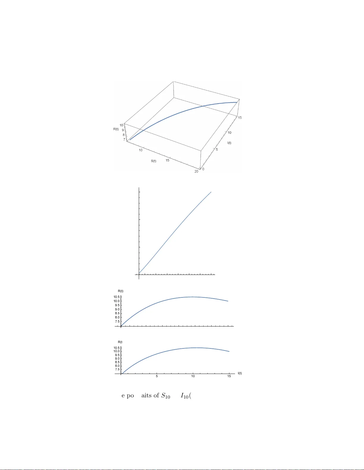
Numerical appro ximatio n of mo dified non-linear SIR mo del of computer viruses Samad No eiaghdam ∗ Departmen t of Mathemat ics, Cent ral T eh ran Branch , Islamic Azad Unive rsi t y , T ehran, Iran. Abstract In this pap er, the non-linear mo dified epidemiological mo del of computer vir uses is illus- trated. F or this aim, t wo semi-analytical metho ds, the differential transform metho d (DTM) and the Laplace-Adomia n dec o mposition metho d (LADM) are a pplied. The numerical re- sults are estimated for differen t v a lues of itera tions and co mpa red to the re sults of the LADM and the homotopy a nalysis tra nsform method (HA TM). Also , graphs of residual err ors and phase p ortraits o f approximate solutions for n = 5 , 10 , 15 are demonstr ated. The numerical approximations show the p erformance of the LADM in co mpa rison to the LADM and the HA TM. keywor ds: Non-line ar Su s c eptible-Infe ct e d-R e c over e d m o del, D iffer ential tr ansform metho d, L aplac e tr ansformations, A domian de c omp osition metho d. 1 In tro duction The computer viruses are malw are pr og rams th at ha ve b een able to infect thousands of com- puters and ha v e hurt billions dollar in computers around the w orld. The virus should nev er b e considered to b e harmless and remain in the system. There are sev eral t yp es of viruses that can b e catego rized according to th ei r source, tec hnique, file type that in f ec ts, where they are h iding, the t yp e of damage they en ter, the t yp e of op erating system, or the design on whic h they are attac king. W e can in tro duce some of famous and malicious viruses such as ILO VEYOU, Melissa, My Do om, Cod e Red, Sasser, Stuxnet and so on. Th er efore, it is imp or- tan t that w e stud y the metho ds to analyze, trac k, mo del, and p rotec t aga inst viruses. In recent y ears, man y scientists ha v e b een illustrated the epidemiological mo dels of computer viruses [2, 14 , 17, 21, 32, 33, 36, 37, 45, 46, 47]. These mo dels ha ve b een estimated by many mathe- matical metho ds suc h as col lo cation metho d [30], homotop y analysis metho d [5, 27], v ariational iteration metho d [23] and others [33, 41]. ∗ Corresponding author, E-mail addresses: s.noeiaghdam.sci@iauctb.ac.ir; samadnoeiaghdam@gmail.com T el.: +98 9143527552 1 One of applicable and imp ortant mo dels is th e classical Susceptible-Infected-Reco vered (SIR) computer virus propagation mod el [21, 22, 33] whic h is p resen ted in the follo wing form: dS ( t ) dt = f 1 − λS ( t ) I ( t ) − dS ( t ) , dI ( t ) dt = f 2 + λS ( t ) I ( t ) − εI ( t ) − dR ( t ) , dR ( t ) dt = f 3 + εI ( t ) − dR ( t ) , (1) where S (0) = S 0 ( t ) , I (0) = I 0 ( t ) , R (0) = R 0 ( t ) , (2) are the initial conditions of non-linear sy s te m of Eqs . (1). F unctions and initial v alues of sys te m (1) are giv en in T able 1. T able 1: List of parameters and fun ct ions. P arameters Meaning V alues & F unctions S ( t ) Susceptible computers at time t S (0) = 20 I ( t ) Infected computers at time t I (0) = 15 R ( t ) Reco v ered computers at time t R (0) = 10 f 1 , f 2 , f 3 Rate of extern al computers connected to the n etw ork f 1 = f 2 = f 3 = 0 λ Rate of in fecti ng for sus ceptible computer λ = 0 . 001 ε Rate of r eco very for infected computers ε = 0 . 1 d Rate of r emo vin g fr om the n et work d = 0 . 1 Recen tly , sev eral numerical and semi-analytical metho ds are introd uced to solv e the math- ematical and engineering p roblems [9 , 10, 11 , 24, 25, 26, 48] th at we can ap p ly them to solv e the non-linear mo del (1). The DTM and the LADM are t w o imp ortan t and efficient to ols to solv e the linear and non-linear problems arising in the mathematics, ph ysics and engineering [6, 7, 29 , 34, 35, 40, 43]. Sp ecially , the LADM [12, 15, 31] obtai ned by co mbining the Ad omia n decomp osition metho d [1, 3 , 4, 16, 39, 44] and th e Laplace transformations [18] similar to the HA TM [8, 24, 27, 28], Laplace homotop y p erturbation metho d [13, 38, 42] and so on. The aim of this pap er is to app ly the DTM and the LADM to fin d the app ro ximate solution of non-linear epidemiological system of Eqs. (1). The numerical results are compared w ith the HA TM [8, 24, 27, 28] by plotting the resid u al errors fun ct ion for different iterations. A lso, the phase p ortraits of approximat e solutions for n = 10 and differen t functions of S ( t ) , I ( t ) and R ( t ) are pr esen ted. The n umerical results sho w the abilities and capabilities of th e L AD M in comparison to the DTM and the HA TM. 2 2 Differen tial transform metho d T ransformation of the k -th deriv ativ e of a function in one v ariable is as f ollo ws F ( k ) = 1 k !  d k f ( t ) dt k  t = t 0 , (3) and the inv erse transformation is defined b y f ( t ) = ∞ X k =0 F ( k )( t − t 0 ) k (4) where F ( k ) is the d ifferen tial transform of f ( t ). In actual applications, the function f ( t ) is expressed b y a finite series and E q . (4) can b e rewritten as follo ws: f ( t ) = N X k =0 F ( k )( t − t 0 ) k (5) where N is decided b y the con v ergence of natural fr equency . The f u ndamen tal op erations of DTM ha v e b een giv en in T able 3. T able 2: Main operations of DTM. Original functions T ransformed fu nctions f ( t ) = u ( t ) ± v ( t ) F ( k ) = U ( k ) ± V ( k ) f ( t ) = β u ( t ) F ( k ) = β U ( k ) f ( t ) = u ( t ) v ( t ) F ( k ) = P k i =0 U ( k ) V k − s ( k ) f ( t ) = du ( t ) dt F ( k ) = ( k + 1) U ( k + 1) f ( t ) = d m u ( t ) dt m F ( k ) = ( k + 1)( k + 2) · · · ( k + m ) U ( k + m ) f ( t ) = R t t 0 u ( ξ ) dξ F ( k ) = U ( k − 1) k , k ≥ 1 f ( t ) = t m F ( k ) = δ ( k − m ) f ( t ) = exp( λt ) F ( k ) = λ k k ! f ( t ) = sin( ω t + α ) F ( k ) = ω k k ! sin( π k 2 + α ) f ( t ) = cos( ω t + α ) F ( k ) = ω k k ! cos( π k 2 + α ) 3 By applying the presen ted metho d to system of Eqs. (1), we get S k +1 = 1 k + 1 " f 1 − λ k X i =0 S i I k − i − dS k # , I k +1 = 1 k + 1 " f 2 − λ k X i =0 S i I k − i − εI k − dR k # , R k +1 = 1 k + 1  f 3 − εI k − dR k  . (6) The differen tial transform metho d series solution for system (1) can b e obtained as S ( t ) = n X j =0 S j t j , I ( t ) = n X j =0 I j t j , R ( t ) = n X j =0 R j t j , (7) 3 Laplace-Adomian decomp osition metho d W e apply the Laplace transformation L as L [ S ( t )] = S (0) z + L [ f 1 ] z − λ z L [ S ( t ) I ( t )] − d z L [ S ( t )] , L [ I ( t )] = I (0) z + L [ f 2 ] z + λ z L [ S ( t ) I ( t )] − ε z L [ I ( t )] − d z L [ R ( t )] , L [ R ( t )] = R (0) z + L [ f 3 ] z + ε z L [ I ( t )] − d z L [ R ( t )] . (8) By putting the initial conditions we ha ve L [ S ( t )] = S (0) z + f 1 z 2 − λ z L [ A ] − d z L [ S ( t )] , L [ I ( t )] = I (0) z + f 2 z 2 + λ z L [ A ] − ε z L [ I ( t )] − d z L [ R ( t )] , L [ R ( t )] = R (0) z + f 3 z 2 + ε z L [ I ( t )] − d z L [ R ( t )] , (9) 4 where A = S I and S = ∞ X j =0 S j , I = ∞ X j =0 I j , R = ∞ X j =0 R j . (10) Also, the non-linear op erator A is calle d the Adomian p olynomials and it is presen ted as A = ∞ X j =0 A j , (11) where A 0 = S 0 I 0 , A 1 = S 0 I 1 + S 1 I 0 , A 2 = S 0 I 2 + S 1 I 1 + S 2 I 0 , A 3 = S 0 I 3 + S 1 I 2 + S 2 I 1 + S 3 I 0 , A 4 = S 0 I 4 + S 1 I 3 + S 2 I 2 + S 3 I 1 + S 4 I 0 , . . . (12) By substituting series (10) and (11) int o (9) we get L   ∞ X j =0 S j   = S (0) z + f 1 z 2 − λ z L   ∞ X j =0 A j   − d z L   ∞ X j =0 S j   , L   ∞ X j =0 I j   = I (0) z + f 2 z 2 + λ z L   ∞ X j =0 A j   − ε z L   ∞ X j =0 I j   − d z L   ∞ X j =0 R j   , L   ∞ X j =0 R j   = R (0) z + f 3 z 2 + ε z L   ∞ X j =0 I j   − d z L   ∞ X j =0 R j   . (13) 5 No w, the follo wing relations can b e obtained: L [ S 0 ] = S (0) z + f 1 z 2 , L [ I 0 ] = I (0) z + f 2 z 2 , L [ R 0 ] = R (0) z + f 3 z 2 , L [ S 1 ] = λ z L [ A 0 ] − d z L [ S 0 ] , L [ I 1 ] = λ z L [ A 0 ] − ε z L [ I 0 ] − d z L [ R 0 ] , L [ R 1 ] = ε z L [ I 0 ] − d z L [ R 0 ] , (14) and for term j we h a ve L [ S j ] = λ z L [ A j − 1 ] − d z L [ S j − 1 ] , L [ I j ] = λ z L [ A j − 1 ] − ε z L [ I j − 1 ] − d z L [ R j − 1 ] , L [ R j ] = ε z L [ I j − 1 ] − d z L [ R j − 1 ] . (15) Applying the in v erse Laplace transformation L − 1 for first equations of (14) as follo w s S 0 = S (0) + f 1 t, I 0 = I (0) + f 2 t, R 0 = R (0) + f 3 t, (16) 6 By p u tting S 0 , I 0 , R 0 in second equ at ions of (14) and using the L apla ce transform at ions w e ha v e L [ S 1 ] = λ z  S (0) I (0) z + S (0) f 2 z 2 + I (0) f 1 z 2 + 2 f 1 f 2 z 3  − d z  S (0) z + f 1 z 2  , L [ I 1 ] = λ z  S (0) I (0) z + S (0) f 2 z 2 + I (0) f 1 z 2 + 2 f 1 f 2 z 3  − ε z  I (0) z + f 2 z 2  − d z  R (0) z + f 3 z 2  , L [ R 1 ] = ε z  I (0) z + f 2 z 2  − d z  R (0) z + f 3 z 2  , (17) and by applying the inv erse Laplace trans f orm L − 1 w e can find S 1 , I 1 and R 1 . B y rep eati ng ab o v e pro cess, the other terms S 2 , · · · , S j , I 2 , · · · , I j , R 2 , · · · , R j can b e obtained. By using the relations S n = n X j =0 S j , I n = n X j =0 I j , R n = n X j =0 R j , (18) the n -th order app r o ximate solutions can b e estimat ed. 4 Numerical Illustration In this s ec tion, the numerical results of the DTM and the LADM for solving the system of Eqs. (1) are p r esen ted. The approxi mate solutions for n = 5 by using the DTM are obtained in the follo wing form S 5 ( t ) = 20 − 2 . 3 t + 0 . 15425 t 2 − 0 . 00790 458 t 3 + 0 . 00030 9711 t 4 , I 5 ( t ) = 15 − 2 . 2 t + 0 . 04575 t 2 + 0 . 00573 792 t 3 − 0 . 00040 6169 t 4 , R 5 ( t ) = 10 + 0 . 5 t − 0 . 135 t 2 + 0 . 00602 5 t 3 − 7 . 17708 × 10 − 6 t 4 , 7 and for n = 10 we ha v e S 10 ( t ) = 20 − 2 . 3 t + 0 . 15425 t 2 − 0 . 00790 458 t 3 + 0 . 00030 9711 t 4 − 7 . 74864 × 10 − 6 t 5 − 1 . 35996 × 10 − 8 t 6 + 1 . 41005 × 10 − 8 t 7 − 8 . 93373 × 10 − 10 t 8 + 3 . 32927 × 10 − 11 t 9 , I 10 ( t ) = 15 − 2 . 2 t + 0 . 04575 t 2 + 0 . 00573 792 t 3 − 0 . 00040 6169 t 4 + 9 . 82135 × 10 − 6 t 5 + 1 . 12052 × 10 − 7 t 6 − 1 . 97453 × 10 − 8 t 7 + 9 . 96904 × 10 − 10 t 8 − 3 . 2067 × 10 − 11 t 9 , R 10 ( t ) = 10 + 0 . 5 t − 0 . 135 t 2 + 0 . 00602 5 t 3 − 7 . 17708 × 10 − 6 t 4 − 7 . 97984 × 10 − 6 t 5 + 2 . 96686 × 10 − 7 t 6 − 2 . 63764 × 10 − 9 t 7 − 2 . 13846 × 10 − 10 t 8 + 1 . 34528 × 10 − 11 t 9 , and finally for n = 15 the appro ximate solutions are obtai ned as S 15 ( t ) = 20 − 2 . 3 t + 0 . 15425 t 2 − 0 . 00790 458 t 3 + 0 . 00030 9711 t 4 − 7 . 74864 × 10 − 6 t 5 − 1 . 35996 × 10 − 8 t 6 + 1 . 41005 × 10 − 8 t 7 − 8 . 93373 × 10 − 10 t 8 + 3 . 32927 × 10 − 11 t 9 − 5 . 68453 × 10 − 13 t 10 − 2 . 34166 × 10 − 14 t 11 + 2 . 59234 × 10 − 15 t 12 − 1 . 28786 × 10 − 16 t 13 + 3 . 788 68 × 10 − 18 t 14 , I 15 ( t ) = 15 − 2 . 2 t + 0 . 04575 t 2 + 0 . 005 73792 t 3 − 0 . 00040 6169 t 4 + 9 . 82135 × 10 − 6 t 5 + 1 . 12052 × 10 − 7 t 6 − 1 . 97453 × 10 − 8 t 7 + 9 . 96904 × 10 − 10 t 8 − 3 . 2067 × 10 − 11 t 9 + 4 . 21668 × 10 − 13 t 10 + 2 . 88892 × 10 − 14 t 11 − 2 . 70438 × 10 − 15 t 12 + 1 . 28307 × 10 − 16 t 13 − 3 . 627 09 × 10 − 18 t 14 , R 15 ( t ) = 10 + 0 . 5 t − 0 . 135 t 2 + 0 . 00602 5 t 3 − 7 . 17708 × 10 − 6 t 4 − 7 . 97984 × 10 − 6 t 5 + 2 . 96686 × 10 − 7 t 6 − 2 . 63764 × 10 − 9 t 7 − 2 . 13846 × 10 − 10 t 8 + 1 . 34528 × 10 − 11 t 9 − 4 . 55198 × 10 − 13 t 10 + 7 . 97151 × 10 − 15 t 11 + 1 . 74314 × 10 − 16 t 12 − 2 . 21438 × 10 − 17 t 13 + 1 . 074 65 × 10 − 18 t 14 . 8 No w, b y applyin g the LADM w e get S 0 ( t ) = 20 , I 0 ( t ) = 15 , R 0 ( t ) = 10 , S 1 ( t ) = − 2 . 3 t, I 1 ( t ) = − 2 . 2 t, R 1 ( t ) = 0 . 5 t, S 2 ( t ) = 0 . 15425 t 2 , I 2 ( t ) = 0 . 045 75 t 2 , R 2 ( t ) = − 0 . 135 t 2 , . . . . . . . . . S 10 ( t ) = − 5 . 68453 × 10 − 13 t 10 , I 10 ( t ) = 4 . 21668 × 10 − 13 t 10 , R 10 ( t ) = − 4 . 55198 × 10 − 13 t 10 , . . . . . . . . . and finally the appro ximate solution of epidemiological mo del of computer viruses (1) for n = 10 is in th e follo wing form S 10 ( t ) = 10 X j =0 S j ( t ) = 20 − 2 . 3 t + 0 . 15425 t 2 − 0 . 00790 458 t 3 + 0 . 000 309711 t 4 − 7 . 74864 × 10 − 6 t 5 − 1 . 35996 × 10 − 8 t 6 + 1 . 41005 × 10 − 8 t 7 − 8 . 93373 × 10 − 10 t 8 + 3 . 32927 × 10 − 11 t 9 − 5 . 68453 × 10 − 13 t 10 , I 10 ( t ) = 10 X j =0 I j ( t ) = 15 − 2 . 2 t + 0 . 04575 t 2 + 0 . 00573 792 t 3 − 0 . 00040 6169 t 4 + 9 . 82135 × 10 − 6 t 5 + 1 . 12052 × 10 − 7 t 6 − 1 . 97453 × 10 − 8 t 7 + 9 . 96904 × 10 − 10 t 8 − 3 . 2067 × 10 − 11 t 9 + 4 . 21668 × 10 − 13 t 10 , R 10 ( t ) = 10 X j =0 R j ( t ) = 10 + 0 . 5 t − 0 . 135 t 2 + 0 . 00602 5 t 3 − 7 . 17708 × 10 − 6 t 4 − 7 . 97984 × 10 − 6 t 5 + 2 . 96686 × 10 − 7 t 6 − 2 . 63764 × 10 − 9 t 7 − 2 . 13846 × 10 − 10 t 8 + 1 . 34528 × 10 − 11 t 9 − 4 . 55198 × 10 − 13 t 10 . In order to show the accuracy of th e p resen ted metho ds, follo wing residual err ors are pre- sen ted. A lso, the n umerical r esults are compared to the obtained results of the HA T M for 9 n = 5 , 10. The results are presen ted in T ables 3, 4 and 5. E n,S ( t ) = S ′ n ( t ) − f 1 + λS n ( t ) I n ( t ) + dS n ( t ) , E n,I ( t ) = I ′ n ( t ) − f 2 − λS n ( t ) I n ( t ) + εI n ( t ) + dR n ( t ) , E n,R ( t ) = R ′ n ( t ) − f 3 − εI n ( t ) + dR n ( t ) . (19) The comparativ e graph s b et we en the residual errors of the LADM, the DTM and the HA TM for n = 5 , 10 , 15 are demonstrated in Figs. 1, 2 and 3. Also, phase p ortraits of S − I , S − R, I − R and S − I − R whic h are obtained b y 10-th order approximat ion of the DTM and the LADM are present ed in Figs. 4 and 5. According to the generated results, the LADM has su itable scheme than the DTM and the HA T M. T able 3: Numerical comparison of r esidual error E n,S ( t ) b et w een LADM, DTM and HA TM f or n = 5 , 10. t E 5 ,S ( t )-LADM E 5 ,S ( t )-DTM E 5 ,S ( t )-HA TM E 10 ,S ( t )-LADM E 10 ,S ( t )-DTM E 10 ,S ( t )-HA TM 0 . 0 0 0 0 0 0 0 0 . 2 1 . 98295 × 10 − 11 6 . 22316 × 10 − 8 0 . 0000116 327 4 . 44089 × 10 − 16 4 . 44089 × 10 − 16 4 . 22713 × 10 − 11 0 . 4 4 . 38413 × 10 − 10 9 . 99398 × 10 − 7 0 . 0000188 901 0 1 . 7763 6 × 10 − 15 8 . 71449 × 10 − 10 0 . 6 1 . 87637 × 10 − 9 5 . 07724 × 10 − 6 0 . 0000214 386 1 . 77636 × 10 − 15 5 . 9508 × 10 − 14 4 . 95175 × 10 − 9 0 . 8 1 . 93464 × 10 − 9 0 . 0000161 0 . 00015492 2 . 57572 × 10 − 14 7 . 94032 × 10 − 13 1 . 57635 × 10 − 8 1 . 0 1 . 18760 × 10 − 8 0 . 0000394 305 0 . 0004295 09 2 . 30038 × 10 − 13 5 . 97122 × 10 − 12 3 . 43742 × 10 − 8 T able 4: Numerical comparison of residu al error E n,I ( t ) b et w een L ADM , DTM and HA TM for n = 5 , 10. t E 5 ,I ( t )-LADM E 5 ,I ( t )-DTM E 5 ,I ( t )-HA TM E 10 ,I ( t )-LADM E 10 ,I ( t )-DTM E 10 ,I ( t )-HA TM 0 . 0 0 0 7 . 10543 × 10 − 15 0 0 0 0 . 2 2 . 08857 × 10 − 10 7 . 88132 × 10 − 8 0 . 0000138 59 4 . 44089 × 10 − 16 4 . 44089 × 10 − 16 4 . 24451 × 10 − 11 0 . 4 6 . 48732 × 10 − 9 1 . 26470 × 10 − 6 0 . 0000368 61 4 . 44089 × 10 − 16 1 . 77636 × 10 − 15 8 . 8009 × 10 − 10 0 . 6 4 . 78103 × 10 − 8 6 . 42035 × 10 − 6 0 . 0000397 647 1 . 77636 × 10 − 15 4 . 44089 × 10 − 14 5 . 06861 × 10 − 9 0 . 8 1 . 95500 × 10 − 7 0 . 0000203 449 8 . 51494 × 10 − 6 3 . 15303 × 10 − 14 5 . 96412 × 10 − 13 1 . 65033 × 10 − 8 1 . 0 5 . 78838 × 10 − 7 0 . 0000497 94 0 . 0001409 14 2 . 89546 × 10 − 13 4 . 50395 × 10 − 12 3 . 7476 × 10 − 8 T able 5: Numerical comparison of residual error E n,R ( t ) b et we en LADM, DTM and HA T M for n = 5 , 10. t E 5 ,R ( t )-LADM E 5 ,R ( t )-DTM E 5 ,R ( t )-HA TM E 10 ,R ( t )-LADM E 10 ,R ( t )-DTM E 10 ,R ( t )-HA TM 0 . 0 0 0 0 0 0 0 0 . 2 5 . 69638 × 10 − 10 6 . 38387 × 10 − 8 1 . 95392 × 10 − 6 1 . 11022 × 10 − 16 3 . 33067 × 10 − 16 1 . 04154 × 10 − 12 0 . 4 1 . 82284 × 10 − 8 1 . 02142 × 10 − 6 0 . 0000285 358 3 . 33067 × 10 − 16 1 . 22125 × 10 − 15 8 . 17403 × 10 − 12 0 . 6 1 . 38422 × 10 − 7 5 . 17094 × 10 − 6 0 . 0001128 91 7 . 21645 × 10 − 16 4 . 56857 × 10 − 14 1 . 57476 × 10 − 10 0 . 8 5 . 83309 × 10 − 7 0 . 0000163 427 0 . 0002909 76 9 . 43690 × 10 − 15 6 . 10734 × 10 − 13 1 . 69486 × 10 − 9 1 . 0 1 . 78012 × 10 − 6 0 . 0000398 992 0 . 0006016 21 8 . 77631 × 10 − 14 4 . 55164 × 10 − 12 8 . 65934 × 10 − 9 10 0.2 0.4 0.6 0.8 1.0 t 0.00001 0.00002 0.00003 0.00004 0.00005 0.00006 E 5, S ( t ) E 5, S ( t )- HATM E 5, S ( t )- DTM E 5, S ( t )- LADM 0.2 0.4 0.6 0.8 1.0 t 0.00002 0.00004 0.00006 0.00008 E 5, I ( t ) E 5, I ( t )- HATM E 5, I ( t )- DTM E 5, I ( t )- LADM 0.2 0.4 0.6 0.8 1.0 t 0.00002 0.00004 0.00006 0.00008 0.00010 E 5, R ( t ) E 5, R ( t )- HATM E 5, R ( t )- DTM E 5, R ( t )- LADM Figure 1: Comparison b et we en error fun cti ons of LADM, DTM and HA TM for S 5 ( t ) , I 5 ( t ) , R 5 ( t ). 11 0.2 0.4 0.6 0.8 1.0 t 1. × 10 - 9 2. × 10 - 9 3. × 10 - 9 4. × 10 - 9 E 10, S ( t ) E 10, S ( t )- HATM E 10, S ( t )- DTM E 10, S ( t )- LADM 0.2 0.4 0.6 0.8 1.0 t 1. × 10 - 9 2. × 10 - 9 3. × 10 - 9 4. × 10 - 9 E 10, I ( t ) E 10, I ( t )- HATM E 10, I ( t )- DTM E 10, I ( t )- LADM 0.2 0.4 0.6 0.8 1.0 t 5. × 10 - 12 1. × 10 - 11 1.5 × 10 - 11 2. × 10 - 11 E 10, R ( t ) E 10, R ( t )- HATM E 10, R ( t )- DTM E 10, R ( t )- LADM Figure 2: Comparison b et w een error functions of LADM, DTM and HA TM for S 10 ( t ) , I 10 ( t ) , R 10 ( t ). 12 0.2 0.4 0.6 0.8 1.0 t 5. × 10 - 12 1. × 10 - 11 1.5 × 10 - 11 2. × 10 - 11 E 15, S ( t ) E 15, S ( t )- HATM E 15, S ( t )- DTM E 15, S ( t )- LADM 0.2 0.4 0.6 0.8 1.0 t 5. × 10 - 12 1. × 10 - 11 1.5 × 10 - 11 2. × 10 - 11 2.5 × 10 - 11 E 15, I ( t ) E 15, I ( t )- HATM E 15, I ( t )- DTM E 15, I ( t )- LADM 0.2 0.4 0.6 0.8 1.0 t 5. × 10 - 12 1. × 10 - 11 1.5 × 10 - 11 2. × 10 - 11 2.5 × 10 - 11 E 15, R ( t ) E 15, R ( t )- HATM E 15, R ( t )- DTM E 15, R ( t )- LADM Figure 3: Comparison b et w een error functions of LADM, DTM and HA TM for S 15 ( t ) , I 15 ( t ) , R 15 ( t ). 13 - 15 - 10 - 5 5 10 15 20 S ( t ) - 20 - 10 10 I ( t ) - 15 - 10 - 5 5 10 15 20 S ( t ) - 50 - 40 - 30 - 20 - 10 10 R ( t ) - 20 - 10 10 I ( t ) - 50 - 40 - 30 - 20 - 10 10 R ( t ) Figure 4: Phase p ortraits of S 10 ( t ) , I 10 ( t ) , R 10 ( t ) b y using the LADM. 14 8 10 12 14 16 18 20 S ( t ) 5 10 15 I ( t ) 8 10 12 14 16 18 20 S ( t ) 7  8    9    1      R ( t ) 5 10 15 I ( t )   8.0       10.0  !" R ( t ) Figure 5: Phase p ortraits of S 10 ( t ) , I 10 ( t ) , R 10 ( t ) b y using the DTM. 15 5 Conclusion In th is study , t w o robust and applicable metho ds, the DTM and th e LADM w ere app lie d to solv e the n on-linea r epidemiological mo del of computer viru s es. In ord er to sho w the efficiency and accuracy of presen ted metho d , the residual errors for differen t iterations w ere presen ted based on the LADM, DTM and HA TM. Also, the graph s of residual err or w ere d emonstrate d to sho w the abilities of the LADM than the other method s. References [1] S. Abb asbandy , E xtended Newton’s m et ho d for a system of n onlinear equations b y mo di- fied Adomian decomp osition m et ho d, Ap plied Mathematics and Computation, 170, 648-65 6 (2005 ). [2] F. Cohen, Computer viruses: theory and exp erimen ts, Comput. Secur., 6, 22-3 5 (1987). [3] J.S. Duan, R. Rac h, A.M. W azw az, Higher ord er numeric solutions of the Lane-Emden- t yp e equations d er ived f rom the m ulti-stage mo dified Adomian d ecomp osition metho d, In t. J. Comput. Math., 94(1), 197-215 (2017). [4] A. Ebaid, M. D. Aljoufi, A.M. W azw az, An adv anced study on th e solution of nanofluid flow problems via Adomian’s m ethod, Appl. Math. Lett., 46, 117 -122 (2015). [5] A.A. F reihat, M. Zurigat, A. H. Hand am, The multi- step homotop y analysis metho d for mo dified ep id emio logical mo del for computer viru s es, Afr ik a Matemati k a, 26 (3-4), 585-596 (2015 ). [6] M.A. F arib orzi Araghi, Sh. Behzadi, Solving nonlinear V olterra-F redholm integ ro-differentia l equations using the mo dified Adomian decomp osition method , Computational Metho ds In Applied Mathematic s, 9 (4), 1-11 (20 09). [7] M.A. F arib orzi Araghi, A. F allahzadeh, Dynamical Con trol of accuracy using the sto c hastic arithmetic to estimate the solution of the ordinary differen tial equations via Adomian de- comp ositio n method , Asian Journal of Mathematic s and C omputer Researc h, 8(2) , 128-13 5 (2016 ). [8] M.A. F arib orzi Araghi, S. No eiaghdam, Homotop y analysis transform metho d for solving generalized Ab el’s fu zz y integ ral equ at ions of the first kind, IEEE (2016). [9] M.A. F arib orzi Araghi, S. No eiaghdam, Fib onacci-regularizati on metho d for solving Cauch y in tegral equations of the first kind, Ain Sh ams Eng J., (8), 363- 369 (2017). [10] M. F arib orzi Araghi, S . No eia ghdam, A n o vel tec hn ique based on the homotop y analysis metho d to solv e th e first kind Cauc hy in tegral equations arising in the theory of airfoils, Journal of In terp olatio n and Appro ximation in Scien tific Computing, (1), 1-13 (2016). 16 [11] M.A. F arib orzi Ar ag hi, S. No eiag hd am, Homotop y regularizatio n metho d to solve the sin gu- lar V olterra integ ral equ at ions of the first kind, Jordan Journal of Mathematics and Statistics, 10(4), (2017 ). [12] H.E. Gadian, Solving coupled pseud o-parab olic equation usin g a mo dified d ouble Laplace decomp osition method, Acta Mathematica Scien tia, 38 (1), 333-3 46 (2018 ). [13] S. Gupta, D. Kumar, J. S ingh, Analytical solutions of conv ection-diffusion problems b y com bining Laplace transform metho d and h omot opy p erturb ation method , Alexandria Engi- neering Journal, 54 (3) , 645-651 (2015). [14] X. Han, Q. T an, Dynamical b eha vior of computer viru s on Int ernet, App l. Math. Comput., 217, 2520 -2526 (2010). [15] F. Haq, K. Sh ah , G. ur Rahman, M. Shahzad, Numerical solution of fractional order sm ok- ing mo del via laplace Adomian decomp osition metho d, Alexandria Engineering Jour n al, In press, 13, (20 17). [16] S. Gh . Hosseini, E. Bab ol ian, S. Ab b asbandy , A new algorithm for solving V an der P ol equation based on piecewise sp ectral Adomian d ec omp osition metho d, Int. J. Indu strial Math., 8(3), 177- 184 (2016). [17] J.O. Kephart, T. Hogg, B.A. Hub erman, Dynamics of computational ecosystems, Phys. Rev. A, 40 (1), 404-421 (1998). [18] S. Kumar, D. Kumar, S. Abb asbandy , M.M. Rashidi, An al ytical solution of fr ac tional Na vier-Stok es equation by using mo d ified Laplace decomp osition metho d, Ain Shams Eng. J., 5, 569-574 (2014). [19] S. Kumar, J. Singh, D. Kum ar, S. Kap o or, New homotop y analysis transform algo rithm to solv e v olterra integ ral equation, Ain S hams En g J., 5, 243 -246 (2014). [20] D. K umar, J. Singh, Sushila, Ap plica tion of homotop y an alysis transform metho d to frac- tional biologica l p opulation mo del, Romanian Rep orts in P hysics, 65, 63-75 (2013). [21] B.K. Mishra, N. Jha, Fixed p erio d of temp orary immunit y after run of an ti-malicious soft w are on computer no des, Appl. Math. Compu t., 190, 1207- 1212 (2007). [22] B.K. Mishra, S.K. Pandey , F uzzy epid emic mo del for the transmission of worms in computer net w ork, Nonlinear Anal.: Real W orld Appl., 11, 4335- 4341 (2010). [23] S. No eiag hd am, A no ve l tec hnique to solv e the mo dified epidemiologica l mod el of computer viruses, SeMA Journal, (20 18). https://doi.org/ 10.1007/ s40324-018-0163-3. [24] S. No eiaghdam, Solving a non-linear mo del of HIV inf ection for CD4 + T cells by com bining Laplace transformation and Homo topy analysis method , arXiv:1809.06 232 . 17 [25] S. No eiaghdam, M.A. F arib orzi Araghi, S . Abbasb an d y , Finding optimal conv ergence con- trol parameter in the homotop y analysis metho d to solv e integ ral equations based on the sto c h asti c arithm et ic, Num er Algor, (2018) . https:// doi.org/10.10 07/s11075-018-0546-7. [26] S. No eiag hd am, D. S idoro v, V. Sizik o v, Con trol of accuracy on T a ylor-collocation metho d to solv e the we akly regular V olterra in tegral equations of the fir st kind by us in g the C E ST A C metho d, arXiv:1811.0980 2 v1. [27] S. No eiaghdam, M. Su le man, H. Budak, Solving a mo d ified non lin ea r epidemiologic al mo del of computer viruses b y homotop y analysis method , Mathematical Sciences, 1-12 (2018). [28] S. No eiag hd am, E. Zarei, H. Barzegar Kelishami, Homotop y analysis transform metho d for solving Ab el’s inte gral equations of the firs t k in d, Ain Shams Eng. J., 7, 483 -495 (2016). [29] M. Nourifar, A. Aftabi Sani, A. Keyhani, Efficient multi-step d ifferen tial trans form metho d: Theory and its application to nonlinear oscillato rs, Comm unications in Nonlinear Science and Numerical Sim ulation, 53, 154-1 83 (2017). [30] Y. Ozt ¨ urk, M. G ¨ ulsu, Numerical s olution of a mo dified epid emio logical mo del for computer viruses, Applied Mathematic al Mo delling, 39 (23-24), 7600-761 0 (2015) . [31] S. Paul, S . Pr asa d Mondal, P . Bhattac h ary a, Numerical solution of Lotk a V olterra prey predator mo del b y using Runge-Kutta-F ehlb erg metho d and Laplace Adomian decomp osition metho d, Alexandr ia En gineering Journal, 55 (1), 613 -617 (2016). [32] J.R.C. Piqueira, A.A. de V asconcelos, C.E.C.J. Gabriel, V.O. Araujo, Dynamic m odels for computer viruses, Comput. Secur., 27, 355-359 (2008). [33] J.R.C. Piqueira, V.O. Araujo, A mo dified epidemiological mo del for computer vir uses, Ap pl. Math. Comput., 213 , 355-360 (2009). [34] M.M. Rashidi, E. Erfani, A new analytical study of MHD stagnation-p oin t fl ow in p orous media with heat transfer, C omputers & Fluids, 40, 172-1 78 (2011 ). [35] M.M. Rashidi, E. Erfan i, New analytic al metho d f or solving Burger’s and nonlinear heat transfer equations and comparison with HAM, C omputer Physic s Comm unications, 180, 1539- 1544 (200 9). [36] J. Ren, X. Y ang, L. Y ang, Y. Xu, F. Y ang, A dela y ed computer viru s propagation m o del and its d ynamics, Chaos Soliton F r actal, 45, 74- 79 (2012) . [37] J. Ren, X. Y ang, Q . Zhu, L. Y ang, C. Z hang, A n o vel computer virus mo del and its dynamics, Nonlinear Anal.-Rea l., 3, 376-3 84 (2012) . [38] C. Ro drigue Bam b e Moutsinga, E . Pindza, E. Mar´ e, Homotop y p erturbation transform metho d for pricing un der pur e diffusion mo dels with affine coefficien ts, Journal of K in g S aud Univ ersit y-Science, 30 (1), 1-1 3 (2018). 18 [39] H. Ro ohani Ghehsareh, S. Abbasband y , B. Soltanalizadeh, An alyt ical solutions of the slip Magnetoh ydro dynamik viscous flo w o v er a stretching sheet b y using the Laplace Adomian Decomp osit ion Metho d, Zeitsc h rift fur Naturforsch ung A , 67(a), 248-254 (2012). [40] K. Sh ah, T. S ingh, A. Kili¸ cman, Com bin at ion of integral and pr o jected differenti al trans- form metho ds f or time-fractional gas d y n amics equations, Ain Shams Eng J., In press, (2017 ). [41] J. Singh, D. Ku mar, Z. Hammouch, A. Ata ngana, A fractional epidemiological mo del for computer viru s es p ertaining to a n ew fractional deriv ativ e, Applied Mathematics and Com- putation, 316 (1), 504-515 (2018). [42] M.H. Tiwa na, K . Maqb o ol, A.B. Mann, Homotop y p ertur batio n Laplace transf orm s olution of fractional non-linear r ea ction diffusion system of Lotk a-V olterra t yp e differen tial equation, Engineering Science and T ec hnology , an Internatio nal Journ al, 20 (2), 672- 678 (2017). [43] A.M. W azwa z, Th e com bined Laplace transform-Adomian decomp osition metho d for han- dling nonlinear V olterra integ ro-differentia l equations, Applied Mathematics and Compu ta - tion, 216( 4), 1304-1 309 (2010). [44] A.M. W azw az, R. Rac h, J.S . Duan, Adomian decomp osition metho d for solving the V olterra in tegral form of the Lane-Emden equations with initial v alues and b oundary conditions, Ap - plied Mathemati cs and Computation, 219(1 0), 5004-501 9 (2013). [45] J.C. Wierman, D.J. Marc hette, Mo deling compu ter virus p r ev alence with a susceptible- infected-susceptible mo del with r ein tro duction, Comput. Stat. Data An., 45 , 3-23 (2004). [46] H. Y uan, G. C h en, Net work virus-epidemic mo del with the p oin t-to-group information propagation, Appl. Math. Comput., 20 , 357-367 (2008). [47] Q. Zhu, X. Y ang, J. Ren, Mo deling and analysis of the spr ea d of compu ter virus, C omm u n. Nonlinear Sci. Numer. Sim ul., 17 (12), 5117-5 124 (2012). [48] E. Zarei, S. Noeiaghdam, S olving generalized Ab el’s integ ral equations of the fi rst an d second kinds via T a ylor-collocation metho d, arXiv:1804. 08571 . 19