Practicable Simulation-Free Model Order Reduction by Nonlinear Moment Matching

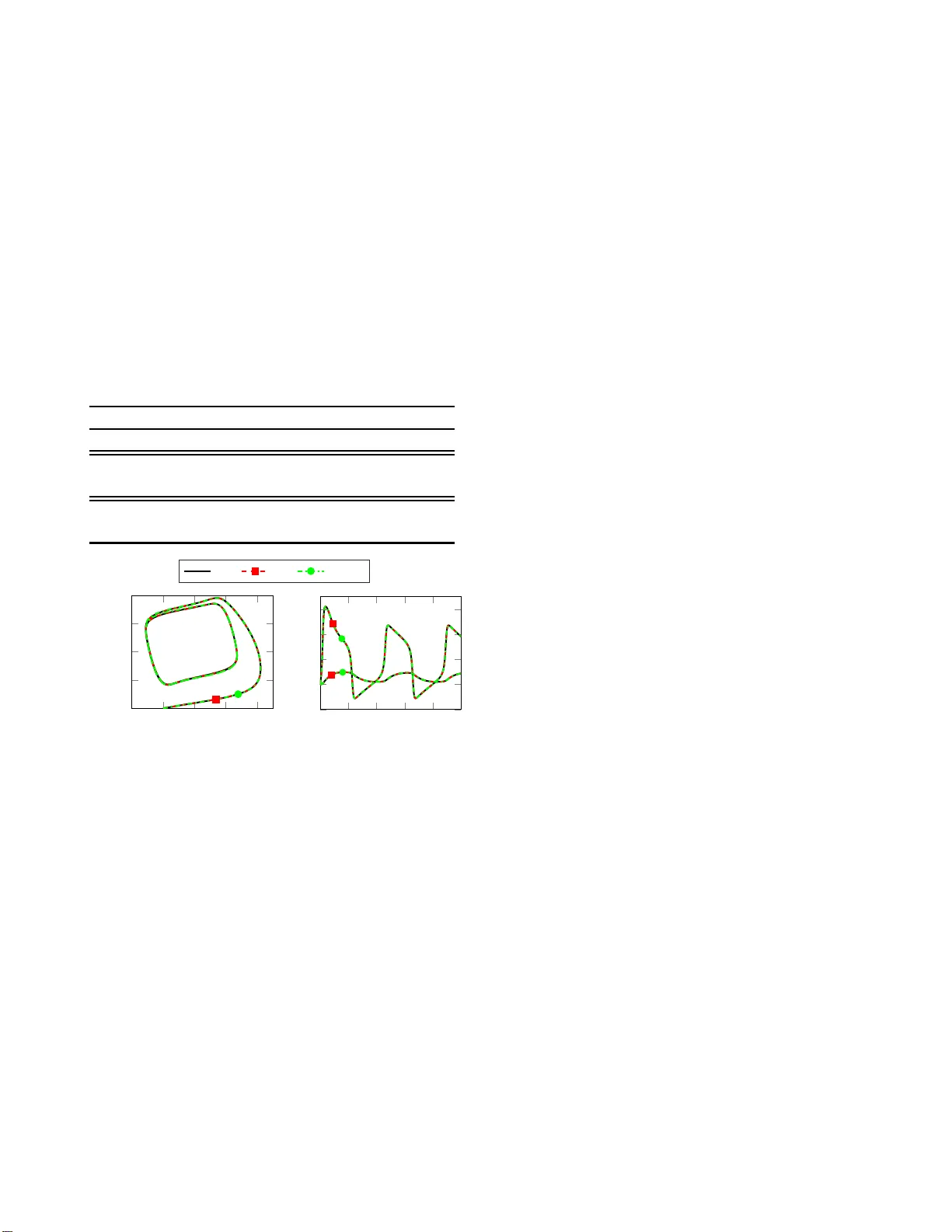
Practicable Simulation-Fr ee Model Order Reduction by Nonlinear Moment Matching M. Cruz V arona, R. Gebhart, J. Suk and B. Lohmann Abstract — In this paper , a practicable simulation-free model order reduction me thod by nonlin ear mom ent matching is deve loped. Based on the steady-state interpretation of lin ear moment matc hing, we compr ehensively ex plain the extension of this reduction concept to nonlinear systems p resented in [1], prov ide some new insights and propose some simplifications to achieve a feasib l e and numerically efficient n onlinear model reduction algorithm. This algorithm r elies on the solution of nonlinear systems of equations ra ther than on the expensiv e simulation of the original model or the difficult solution of a nonlinear partial differential eq uation. I . I N T RO D U C T I O N The detailed mathe matical modelin g of complex dynam- ical systems o ften yields models of thou sands of degrees of f reedom. Since the nu merical simulation and design for such la rge- scale systems is comp u tationally too deman ding, reduced order models that accurate ly appr o ximate the o r igi- nal systems with substantially less effort are stron gly aimed. Nonlinear model order redu ction has been widely studied over the pa st two decades due to the ever increasing in terest in the ef ficient, nume r ical analysis of large-scale nonlinear dynamica l systems. In this r egard, simulation-b a sed red uc- tion tech niques such as Prope r Ortho gonal Decomp osition (POD) [1 8], [16], Trajectory Piecewis e Line a r (TPWL) [1 9], Empirical Gr amians [ 17], Balanc e d-POD [ 24] and Reduced Basis m ethods [10] have established as standard ap proache s. System-theoretic reductio n pro cedures su c h as nonlinear b a- lanced truncation [23] and Krylov sub space methods for special n onlinear system classes [4] h av e been a lso studied. Recently , the conce pt of moment matching an d Kry lov subspaces has b een developed and carried o ver to no nlinear systems [1 ], [2], [12], [13], [21], [22]. From a system- theoretical perspective, this repr e sents a p romising and in- teresting appro a c h tow ards a nonlinea r model reduction technique , wh ich d o es no t rely on the numerical simulation of the original f ull model to c o nstruct the reduced mod el. The exten sion o f the well-kn own concep t of mom ent matching to non lin ear systems has be en initiated by Astolfi [1] a fe w y ears ago based on the theory o f the stead y- state r esponse o f nonlin e a r systems and the tech niques of nonlinear ou tput regulation [15], [14, Ch. 8], [11]. Since then, moment matching for linear and, spec ially , nonlinear systems has been further developed in sev eral publications. For instance, the eq uiv alence be twe e n projectio n-based an d parametrize d , non- p rojective families of reduced models achieving moment m atching is p r esented in [ 2]. Ther e in, the M. Cruz V arona is with the Chair of Automatic Control , Department of Mechani cal Engineeri ng, T ec hnical Un i versit y of Mun ich, Bolt zmannstr . 15, 85748 Garching , Germany . E -mail: maria.cruz@tum.de time doma in interpr etation of outp u t Krylov subspa ce -based moment matching is also established for linear systems using the dual Sylvester equation. These finding s are transferred to the n onlinear case in [1 2] a nd furth er d eveloped in [ 13] to pr ovide a two-side d , n o nlinear m oment match ing theory . More recently , the steady- state interpr etation o f m oments has also been extend ed to linear a n d non lin ear time-delay systems [21]. In ad dition, the on line e stima tion of mom ents of linear and no n linear systems fro m input/outp ut data has ne wly been p roposed in [22]. T his r ecent work aims at th e data- driven, low-ord er identification of an unkn own nonlinear system, by so lving a recursive, movin g window , least-square estimation p roblem using input/o u tput snapshot measuremen ts. Hereby , a po lynomial expansion an satz with user-defined basis functions is used f or the red uced ou tput mapping . Furth ermore, the concep t of parametr ized fami- lies of reduced mo dels is em p loyed to enforce additional proper ties on the reduc e d order m odel, which appr oximately matches the no nlinear, estimated mom ents. From a prac tica l point of v iew , [22] represen ts the first mileston e tow ards a fe a sible m ethod for nonlin ear mo ment matching , since the pr oposed algorithm does not inv olve the solution o f a partial differential equation, but rather aims at estimating th e moment of a nonlinear system from input/o utput data. In fact, the previously mentioned p apers [1], [12], [13], [21] face the same d ifficulty , namely the compu ta tio n of the solutio n of a nonlinear Sylvester-like partial differential eq uation. This paper d evelopes the conce p t o f moment matching for no nlinear system s presente d in [1] tow ards pra c tica l application: In spired by the POD com munity , which usually employs a linear pr ojection and time-snapsho ts to reduc e nonlinear systems, we propo se some simplificatio ns to av oid the Sylvester -like pa rtial d ifferential equatio n and achieve a f easible, numerical algorithm f o r model r eduction b y nonlinear momen t match in g. T he prop osed appr oach is ac- tually linked to the techn ique presented in [ 22] in the sense that both method s ap pr oximately match non lin ear mo m ents. Howe ver , th e goals o f both tech niques are different, since [22] fo cuses on the data-d riv en, low-o rder identifica tio n of an unk nown n onlinear system, wh ereas this p aper deals with the r eduction of a kn own nonlinear system. For this reason, the pr oposed a lgorithms are also different. Algo rithm 2 in [22] requ ires the solution o f a least-square problem using inpu t/output d a ta, whereas the practicable algorithm presented here relies on the solu tion of non linear systems of equations using the exp licitly kn own non linear system. The rest o f the paper is o rgan ized as f ollows. In Section II the theor y of mod el reduction by m o ment matching for linear systems is first revie wed. Here in, the time d omain perception of mome nt match ing f rom [ 1], [2] as th e interp olation of the steady-state respon se of th e output of the system wh en excited by expon e n tial inputs plays a cru cial role for tran sfer- ring this theor y to no nlinear systems. After c ompreh ensiv ely explaining the generalization giv en in [1] and providing some valuable, illuminating insights in Section II I, som e step-b y- step si mplifications are perfo rmed in Section IV towards a practicable , simu la tion-fr ee algorithm for nonlin ear mo ment matching. Finally , a numerical example is provided, which illustrates the effecti veness of the pr oposed metho d. Notatio n: R is the set of real numbers and C is th e set of complex number s. λ ( E − 1 A ) denotes the spectru m of the matrix E − 1 A ∈ R n × n and ∅ repre sen ts the empty set. Finally , the r ange of a ma trix V is denoted by Ran( V ) . I I . M O M E N T M A T C H I N G F O R L I N E A R S Y S T E M S Consider a large-scale, linear time-inv ariant (L TI) , asymp- totically stable, multiple-inp u t multiple-ou tput (MIMO) state-space mod el of the for m E ˙ x ( t ) = A x ( t ) + B u ( t ) , y ( t ) = C x ( t ) , (1) where E ∈ R n × n with det( E ) 6 = 0 is the descriptor matrix, A ∈ R n × n is the system m atrix and x ( t ) ∈ R n , u ( t ) ∈ R m , y ( t ) ∈ R p denote the state, inputs and outputs of the system, respectively . The inp ut-outp ut behavior is characterize d in th e frequen cy domain by the ratio nal transfer function G ( s ) = C ( s E − A ) − 1 B ∈ C p × m . (2) The g oal of mod el ord e r reduction is to ap proxima te the full order mod el (FOM) (1) by a red uced order mo del (R OM) E r ˙ x r ( t ) = A r x r ( t ) + B r u ( t ) , y r ( t ) = C r x r ( t ) , (3) of m u ch smaller dime n sion r ≪ n with E r = W T E V , A r = W T AV , B r = W T B an d C r = C V , su ch that y ( t ) ≈ y r ( t ) . No te that in this framework, the reduction is perfor med by a P etr ov-Galerkin pr ojection of (1) o nto th e r - dimensiona l subsp ace Ran( E V ) by means of the pr o jector P = E V ( W T E V ) − 1 W T . Thus, the main task in th is setting consists in finding suitable ( orthog o nal) p rojection matrices V , W ∈ R n × r that span appr o priate sub spaces. A. Notion of Momen ts a nd Krylov sub spaces One co mmon an d numerically efficient linea r reduction technique relies o n the co ncept of implicit moment matching by ration al Krylov subspaces [ 8], [3]. Definition 1: T h e T aylo r series expansio n of the transfer function G ( s ) aro und a co mplex number σ ∈ C , also called shift or expansion / interpo lation point , is given by G ( s ) = ∞ X i =0 m i ( σ )( s − σ ) i , (4) where m i ( σ ) is called the i -th moment of G ( s ) arou nd σ . The mom ents represen t the T aylor co efficients and satisfy: m i ( σ ) = 1 i ! d i G ( s ) d s i     s = σ = 1 i !  d i d s i C ( s E − A ) − 1 B      s = σ = ( − 1) i C  ( σ E − A ) − 1 E  i ( σ E − A ) − 1 B . If th e matrices V and W are ch osen as b ases of respective r -o rder inp ut an d outp u t rationa l Krylov subspace s K r  ( σ E − A ) − 1 E , ( σ E − A ) − 1 B  ⊆ Ran( V ) , (5 a) K r  ( µ E − A ) − T E T , ( µ E − A ) − T C T  ⊆ Ran( W ) , ( 5b) then the R OM (3) matches r mo ments of the o riginal transfer function aro und the expan sion po ints σ and µ , resp e cti vely . In additio n to the af ore explained mu ltimo ment ma tching strategy , note th at it is also possible to match (high- order) moments at a set of different sh ifts { σ i } q i =1 and { µ i } q i =1 with associated multiplicities { r i } q i =1 , wher e P q i =1 r i = r . In this setting , known as multipoin t mo ment match ing, each subspace Ran( V ) an d Ran( W ) is given by the unio n of all respective rational Kry lov sub spaces K r i . Note also that, b esides th e block Krylov subspaces ( 5), in the MIMO case we alter natively may u se so-called tan gential Krylov subspaces (e.g . for r 1 = . . . = r q = 1 ): span  ( σ 1 E − A ) − 1 B r 1 , . . . , ( σ r E − A ) − 1 B r r  ⊆ Ran( V ) , (6a) span n ( µ 1 E − A ) − T C T l 1 , . . . , ( µ r E − A ) − T C T l r o ⊆ Ran( W ) . ( 6b) Here, conv enient r ight and left tange n tial d ir ections r i ∈ C m and l i ∈ C p are cho sen to tangentially interpo late the tran sfer function at selected expan sion p oints σ i , µ i ∈ C \ λ ( E − 1 A ) . B. Equiva lence o f Krylov subspa ces and Sylvester equatio ns In fact, any basis of an inp ut and outpu t Krylov subspace (6) can be e q uiv alently in terpreted as the solu tion V and W of the following Sylvester eq uations [7]: E V S v − A V = B R , (7a) E T W S T w − A T W = C T L . (7b) Hereby , the inpu t inter p olation data { σ i , r i } is sp ecified by th e matrices S v = dia g( σ 1 , . . . , σ r ) ∈ C r × r and R = [ r 1 , . . . , r r ] ∈ C m × r , where the p air ( R , S v ) is o bservable. Similarly , the ou tp ut interpo lation data { µ i , l i } is d enoted by the matrices S w = diag ( µ 1 , . . . , µ r ) ∈ C r × r and L = [ l 1 , . . . , l r ] ∈ C p × r , where the pair ( S w , L T ) is controllab le. Note that in the multimo m ent case, S v , S w are Jord an matrices, and that in the SISO case 1 , R , L bec o me row vectors with cor r espondin g ones a n d zeros. C. T ime do main interpr etation of Moment Matching In addition to the frequen cy dom ain p erception of mo m ent matching b y means o f the in terpolation of the or ig inal transfer function around certain sh ifts, o ne can also in te r pret this concept in th e time d omain. T o this end , mo ments will be first ch aracterized in ter ms of the solution o f a Sy lvester equation in Lemma 1, an d then interpreted as th e steady-state response of an interconn ected system in Th eorem 1 [1], [2]. Lemma 1: Th e mo ments m i ( σ ) of system (1) aroun d shifts σ 6∈ λ ( E − 1 A ) ar e equiv alently g iv en by m i ( σ ) = ( − 1) i C V i , i = 0 , . . . , r − 1 (8) where, acc o rding to ( 5 a), V i is ca lc u lated as 1 For SISO ( m = 1 , p = 1 ) replace B → b ∈ R n and C → c T ∈ R 1 × n . ˙ x v r ( t ) = S v x v r ( t ) u ( t ) = R x v r ( t ) E ˙ x ( t ) = A x ( t ) + B u ( t ) y ( t ) = C x ( t ) W T E V ˙ x r ( t ) = W T AV x r ( t ) + W T B u ( t ) y r ( t ) = C V x r ( t ) u ( t ) = R e S v t x v r , 0 y ( t ) y r ( t ) e ( t ) = 0 x v r , 0 6 = 0 x 0 = V x v r , 0 x r , 0 = ( W T E V ) − 1 W T E x 0 linear signal generator FOM ROM − Fig. 1: Diagram depicti ng the intercon nection between the linea r FOM/R OM and the linear signal generat or to illustra te t he time domain interpre tatio n of moment matching for linear systems. ( σ E − A ) V 0 = B , ( σ E − A ) V i = E V i − 1 , i ≥ 1 (9) or , alternativ ely , V = [ V 0 , . . . , V r − 1 ] corresp o nds to th e unique solution of the Sylvester equation (7a) with the correspo n ding “modified” Jordan matrix S v with ne gative off-diagonal squar e blocks an d R =  I m 0 m · · · 0 m  . Theor em 1: [1] Consider the inter connectio n of sy stem (1) with the sign al generato r ˙ x v r ( t ) = S v x v r ( t ) , x v r (0) = x v r , 0 6 = 0 , u ( t ) = R x v r ( t ) , (10) where the triple ( S v , R , x v r , 0 ) is such that ( R , S v ) is ob- servable, λ ( S v ) ∩ λ ( E − 1 A ) = ∅ and ( S v , x v r , 0 ) is excitab le . Then, the moments of system (1) are related to the (well- defined) steady- state r e sp onse of the ou tput y ( t ) = y r ( t ) = C V x v r ( t ) of such inte r connected system (cf. Fig 1), wh ere V is the unique solution of th e Sylvester eq uation (7a). Cor ollary 1: Inter c onnecting system (1) with the signa l generato r (10) is equivalent to exciting the FOM with ex- ponen tial inpu t signals u ( t ) = R x v r ( t ) = R e S v t x v r , 0 with exponents given by the shift m atrix S v . Consequently , gi ven u ( t ) = R e S v t x v r , 0 with x 0 = V x v r , 0 , x v r , 0 6 = 0 arbitrary , V as solution of (7a) and W such that det( W T E V ) 6 = 0 , then th e (asym ptotically stable) ROM (3) exactly match es the steady- state re sp onse of the outpu t o f the FOM, i.e. e ( t ) = y ( t ) − y r ( t ) = C x ( t ) − C V x r ( t ) = 0 ∀ t (see Fig. 1). Thus, linear mom ent m a tc h ing can be interpreted as the interpolatio n o f the steady-state response of the output of the FOM, when this is excited with exponential input signals. This under standing follows fr o m the fact that th e tr ansfer function G ( s ) repre sen ts the scaling factor of ( complex) ex- ponen tials e st , wh ich are the eigenfunctions of L T I systems, i.e. y ( t ) = G ( s ) e st for u ( t ) = e st . In terestingly eno ugh, the Sylvester eq uation ( 7a) can be altern ativ ely derived using this time doma in percep tion an d th e no tion of signal generato rs. T o this end , first insert the linear a pprox im ation ansatz x ( t ) = V x r ( t ) with x r ( t ) ! = x v r ( t ) in the state equa tion of (1): E V ˙ x v r ( t ) = A V x v r ( t ) + B u ( t ) . (11) Subsequen tly , th e linear signal g enerator ˙ x v r ( t ) = S v x v r ( t ) , u ( t ) = R x v r ( t ) is plugg ed into (1 1), yielding 0 = ( A V − E V S v + B R ) · x v r ( t ) . (12) Since the eq uation hold s for x v r ( t ) = e S v t x v r , 0 , the state vector x v r ( t ) can b e factored o ut and a constan t ( state-indepen dent) linear Sylvester equ ation of dim ension n × r is obtaine d A V − E V S v + B R = 0 , (13) whose solu tion V spa n s a correspo n ding in p ut rational Krylov subspac e which guaran tees mo ment match ing un der the af orementio ned circumstan ces. I I I . M O M E N T M A T C H I N G F O R N O N L I N E A R S Y S T E M S A. Nonlinear P etr ov-Galerkin pr ojection Consider now a large-scale, no nlinear time-inv ariant, ex- ponen tially stable, MIMO state-space mo d el o f the form ˙ x ( t ) = f  x ( t ) , u ( t )  , x (0) = x 0 , y ( t ) = h  x ( t )  , (14) with x ( t ) ∈ R n , u ( t ) ∈ R m , y ( t ) ∈ R p and smooth mapping s f ( x , u ) : R n × R m → R n and h ( x ) : R n → R p , such that f ( 0 , 0 ) = 0 an d h ( 0 ) = 0 . The aim now is to find a nonlinear ROM of dimension r ≪ n using again a projection framework. One established an d successful way to do th is, is b y apply in g the classical Petrov-Galerkin p r ojection with linear mappin gs g i ven by the matrices V , W to th e n onlinear system (1 4). He rein, the pr o jection matrices ar e g enerally constructed v ia POD or o th er non linear reductio n techn iq ues. Another possibility is to apply a n onlinear Petrov-Galerk in projection using nonlin e ar mappings defined on ma nifolds [13]. T o this end, let x ( t ) = ν ( x r ( t )) be the non linear approx imation an satz with smooth mapp ing ν ( x r ) : R r → R n . Furthermor e , defin e x r ( t ) = ω ( x ( t )) with smooth mapping ω ( x ) : R n → R r , suc h that ω ( ν ( x r )) = x r . The r e duction is th en per formed thro ugh a nonline a r Petrov- Galerkin pro jection  ( x ( t )) = ν  ω ( x ( t ))  of (14) b y means of the pro jector m apping  ( x ) : R n → R n , yieldin g the nonlinear ROM ˙ x r ( t ) = ∂ ω ( x ( t )) ∂ x ( t ) f  x ( t ) , u ( t )      x ( t )= ν ( x r ( t )) , y r ( t ) = h  ν ( x r ( t ))  , (15) where x r ( t ) ∈ R r , ( ∂ ω ( x ) /∂ x ) | x = ν ( x r ) · ( ∂ ν ( x r ) /∂ x r ) = I r and the initial co n dition is x r (0) = ω ( x 0 ) . Remark 1: Th e afore explained nonlinear projection framework ( f or E = I ) is a generalizatio n from the linear case. T herefor e, the non linear mappin gs are strongly related to the ir linear co unterpar ts: x = ν ( x r ) b = V x r , ∂ ν ( x r ) ∂ x r b = V , (16a) x r = ω ( x ) b = ( W T V ) − 1 W T | {z } ∗ x , ∂ ω ( x ) ∂ x b = ∗ , (16b)  = ν  ω ( x )  b = P x , ∂ ν ( x r ) ∂ x r ∂ ω ( x ) ∂ x b = P . (16c) Note that th e c o ndition ω ( ν ( x r )) = x r correspo n ds to ( W T V ) − 1 W T V x r = x r and that P = V ( W T V ) − 1 W T . For nonlin ear systems, a one-sided projection ( W = V ) is commo nly used, which yields ∗ = V T , P = V V T and x r , 0 = V T x 0 , pr ovided tha t V is ortho gonal ( V T V = I r ). ˙ x v r ( t ) = s v  x v r ( t )  u ( t ) = r  x v r ( t )  ˙ x ( t ) = f  x ( t ) , u ( t )  y ( t ) = h  x ( t )  ˙ x r ( t ) = ∂ ω ( x ) ∂ x     x = ν ( x r ) f  ν ( x r ( t )) , u ( t )  y r ( t ) = h  ν ( x r ( t ))  u ( t ) y ( t ) y r ( t ) e ( t ) = 0 x v r , 0 6 = 0 x 0 = ν ( x v r , 0 ) x r , 0 = ω ( x 0 ) nonlinear signal generator FOM ROM − Fig. 2: Diagram depicting the interconnect ion betwee n the nonlinear FOM/R OM and the nonlinea r signal generator to illustra te the time domain interpre tatio n of moment matching for nonlinear systems. B. Notion of Nonline ar Moments The notion o f moments and th eir steady-state-based inter- pretation can be ca r ried over to nonlin ear systems [1]. Theor em 2: [1] Consider the inter connectio n of sy stem (14) with the nonlinea r signal gener a tor ˙ x v r ( t ) = s v  x v r ( t )  , x v r (0) = x v r , 0 6 = 0 , u ( t ) = r  x v r ( t )  , (17) where s v ( x v r ) : R r → R r , r ( x v r ) : R r → R m are smo oth mapping s such that s v ( 0 ) = 0 and r ( 0 ) = 0 . Her eby it is as- sumed, that the signal generato r ( r , s v , x v r , 0 ) is observable, i.e. fo r any pair of initial co nditions x v r , a (0) 6 = x v r , b (0) , the correspo n ding trajectorie s r ( x v r , a ( t )) and r ( x v r , b ( t )) do not coincide. In additio n , the signal generato r (17) can be Poisson stable in a neighb orhoo d of its eq uilibrium x v r = 0 with x v r (0) 6 = 0 . Fur ther assum e that the zero equ ilibrium of the system ˙ x = f ( x , 0 ) is locally expo nentially stable. Th en, the moments of system (14) at ( s v ( x v r ) , r ( x v r ) , x v r , 0 ) are related to the ( locally well-defined ) steady-state respo nse o f the output y ( t ) = y r ( t ) = h  ν ( x v r ( t ))  of such interconnected system (cf . Fig. 2), wh e r e the mapp in g ν ( x v r ) , define d in a n eighbo r hood o f x v r = 0 , is the u nique solutio n of the following Sylvester-like par tial differential eq uation (PDE) ∂ ν ( x v r ) ∂ x v r s v ( x v r ) = f  ν ( x v r ) , r ( x v r )  . (18) C. Stead y-State-Ba sed Nonlin ear Moment Matching Based o n Theorem 2, th e p erception o f no nlinear mo m ent matching in terms of the interpolation of th e stead y-state response o f an inter c onnected system f ollows. Cor ollary 2: Consider the intercon n ection of system ( 14) and the nonline a r signal g enerator (17). Sup pose all assump- tions concer n ing observability and lo cal exponential stability from above h old. Moreover , let ν ( x v r ) be the unique solution of ( 1 8) and ω ( x ) such th at ω ( ν ( x v r )) = x v r . Assume that the zero equilibr ium of (15) is locally expon entially stable. Then, the ROM (1 5) exactly matches the steady-state respon se of the o utput of the FOM, i.e. e ( t ) = y ( t ) − y r ( t ) = h  x ( t )  − h  ν ( x r ( t ))  = 0 ∀ t (see Fig. 2). Note that the Sylvester-like PDE from ( 18) r epresents the nonlinear co unterpar t of the linear equation (1 2): V S v e S v t x v r , 0 = A V e S v t x v r , 0 + B R e S v t x v r , 0 . (19) Thus, the PDE can be alterna tively derived as follows. First, the nonlin ear approxim a tion ansatz x ( t ) = ν ( x r ( t )) with x r ( t ) ! = x v r ( t ) is inserted in the state equation of (14): ∂ ν ( x v r ( t )) ∂ x v r ( t ) ˙ x v r ( t ) = f  ν ( x v r ( t )) , u ( t )  . (20) Afterwards, the nonlinear signal generator ˙ x v r ( t ) = s v  x v r ( t )  , u ( t ) = r  x v r ( t )  is plug ged into (2 0), yielding ∂ ν ( x v r ( t )) ∂ x v r ( t ) s v  x v r ( t )  = f  ν ( x v r ( t )) , r ( x v r ( t ))  . (21) Note that – in contrast to the linear, state- in depend ent Sylvester equation (7a) o f d imension n × r – the PDE (21) is a nonlinea r , state-depen d ent equatio n of d imension n × 1 . I V . S I M U L AT I O N - F R E E N O N L I N E A R M O D E L R E D U C T I O N B Y M O M E N T M AT C H I N G The app roach for nonlinear mom ent matchin g d escribed in Section III r equires the solution ν ( x v r ( t )) of the non linear, state-depend ent PDE (21) for a given signal gen erator, in order to redu ce the FOM (14). This inv olves either sym bolic computatio ns, or the numerical integration of a resulting sys- tem o f or dinary differential equation s (ODEs) after red u ced state-space d iscretization of the PDE (2 1). Since we aim to reduce large-scale nonlin ear systems, almost only num e rical methods come into consideration , which pr e ferably should also av oid an expen si ve simulation. Henc e , some step- by- step simplifications are p erform ed in the following towards a practicable, simulation- f ree method for no nlinear m o ment matching, which relies on the so lu tion o f a system of nonlinear a lgeb raic equatio n s rath er than o f a PDE. A. Linear Pr ojection The first step to wards a p r actical m ethod consists in ap p ly- ing the linear pr ojection ansatz x ( t ) = ν ( x v r ( t )) = V x v r ( t ) instead of the no nlinear projec tio n m a pping ν ( x v r ( t )) . This simplification is motiv ated by the fact th at non linear p ro- jections are much mor e inv olved than linear one s, and that the latter are su c cessfully employed even in nonlinear mod el order redu ction. By doing so, the PDE (2 1) also beco mes an algebra ic e q uation, wh ich is muc h easier to han dle. Dependin g on the fo rm of the used signal generato r , we distinguish ( b ased on [1]) between the following cases: 1) Nonlinea r sig n al generator: In this case, the PDE (2 1) becomes th e following n onlinear system o f equatio ns 0 = f  V x v r ( t ) , r ( x v r ( t ))  − V s v  x v r ( t )  , (22) where the trip le ( s v ( x v r ( t )) , r ( x v r ( t )) , x v r , 0 ) is user-defined and the pr ojection matrix V ∈ R n × r is the searched so lu tion. Note, howe ver , that system (22) consists of n equ ations for n · r u nknowns, i.e. it is und erdetermin e d. Thu s, we co nsider the eq uation column-wise for each v i ∈ R n , i = 1 , . . . , r 0 = f  v i x v r ,i ( t ) , r i ( x v r ,i ( t ))  − v i s v i  x v r ,i ( t )  , (23) with x v r ,i ( t ) ∈ R a n d V = [ v 1 , . . . , v r ] . Please bea r in mind that, in the linear setting, a column- wise construc tio n of the orthog onal basis V using the Arnold i pro cess still fulfills the Sylvester matrix equation (7a). I n the no n linear setting, howe ver , this do es not hold tru e anymo re, since equation (2 2) is g enerally not satisfied, e ven if each colu mn v i fulfills (23). This shortco m ing is a conseque n ce of the usage of a linear projection instead of a non linear mappin g on a man ifold. 2) Linear signal generator: Motiv ated fro m the linear case, one m a y also co me to the id ea of inter c onnecting the nonlinear system ( 14) with th e linear signal gen e rator (10), where s v ( x v r ( t )) = S v x v r ( t ) an d r ( x v r ( t )) = R x v r ( t ) . By doing so, equatio n ( 22) becom es 0 = f  V x v r ( t ) , R x v r ( t )  − V S v x v r ( t ) , (24) where the trip le ( S v , R , x v r , 0 ) is user-defined. Rememb e r that the u sage of a linear signal gen erator correspo nds to exciting the n onlinear system with expo nential input sig- nals u ( t ) = R x v r ( t ) = R e S v t x v r , 0 . This cho ice natu rally raises the question whethe r (gr owing) exponential inpu ts ar e sufficiently valid for character izing nonlinea r systems. N o te that the dynam ics of the selected signal g enerator represent the d ynamics of the nonlinea r system for which th e steady - state respo nses are matched. Th erefore, th e signal generato r should ideally be chosen such that it excites and characte- rizes the important d ynamics of the non linear system. It is well known that expo nential fun c tio ns are the ch a racterizing eigenfun ctions fo r linear systems. By exciting the non linear system with exponential input sign a ls, we ther efore h ope to describe the nonline ar d ynamics adequ ately as well. Considering the underd etermined eq uation again colu m n- wise delivers 0 = f  v i x v r ,i ( t ) , r i x v r ,i ( t ) | {z } r i ( x v r ,i ( t ) )  − v i σ i x v r ,i ( t ) | {z } s v i ( x v r ,i ( t ) ) , (25) where the signal gen e r ator (1 0) becomes ˙ x v r ,i ( t ) = σ i x v r ,i ( t ) , u i ( t ) = r i x v r ,i ( t ) with x v r ,i ( t ) = e σ i t x v r , 0 ,i for i = 1 , . . . , r . 3) Zer o sign al generator: This special ( lin ear) signa l gen- erator is defined as ˙ x v r ( t ) = s v ( x v r ( t )) = 0 , which means that x v r ( t ) = x v r , 0 = c onst and u ( t ) = Rx v r ( t ) = R x v r , 0 = c onst. Hence, the usage of a zer o sign a l gen e r ator is equ iv alent to exciting the nonlinea r system with a constant inp ut sign al. In this particular case, equa tio n ( 22) becom es 0 = f  V x v r , 0 , R x v r , 0  , (26) which is a n o nlinear, time-inde p endent system of equatio ns. A colu mn-wise con sideration of the underd etermined equation yield s 0 = f  v i x v r , 0 ,i , r i ( x v r , 0 ,i ) z }| { r i x v r , 0 ,i  , (27) where ˙ x v r ,i ( t ) = 0 with σ i = 0 , u i ( t ) = r i x v r , 0 ,i = const and x v r ,i ( t ) = x v r , 0 ,i = co nst hold for i = 1 , . . . , r . In o ther words, the em p loyment of a z e ro signal gen erator corresp o nds to moment match ing at shifts σ i = 0 . B. T ime d iscr etization with collo cation p oints Except f or the case with a zero sign al gen erator, the nonlinear equation s (23) and (2 5) ar e state- depende nt and cannot be solved so ea sily . Remem ber that in the linear case, the state vector x v r ( t ) could be factor ed ou t, yielding a con stant linear matrix equatio n th a t is satisfied fo r x v r ( t ) . Unfortu n ately , th is factorization cannot be generally d one in the nonlinear setting anymore. Th us, inspir ed by POD, we propo se to discretize the state-depen dent equatio ns with time- snapshots o r collocatio n poin ts { t ∗ k } , k = 1 , . . . , K . 1) Nonlinea r signal generator: For a time-d iscretized nonlinear signal gener ator s v i ( x v r ,i ( t ∗ k )) , r i ( x v r ,i ( t ∗ k )) and x v r , 0 ,i , the following tim e -indepen dent equatio n r esults 0 = f  v ik x v r ,i ( t ∗ k ) , r i ( x v r ,i ( t ∗ k ))  − v ik s v i  x v r ,i ( t ∗ k )  , (28) which can be solved for each v ik ∈ R n , with i = 1 , . . . , r and k = 1 , . . . , K , if desired. Note that the discrete solutio n x v r ,i ( t ∗ k ) of the nonlinear signal gener ator ODE m ust be given or com p uted via simulatio n befo r e solv ing equ ation (28). 2) Linear signal generator: Using the time-discre tize d signal g e nerator ˙ x v r ,i ( t ∗ k ) = σ i x v r ,i ( t ∗ k ) , u i ( t ∗ k ) = r i x v r ,i ( t ∗ k ) and x v r , 0 ,i , equation ( 25) bec o mes tim e-indepen dent 0 = f  v ik x v r ,i ( t ∗ k ) , r i x v r ,i ( t ∗ k )  − v ik σ i x v r ,i ( t ∗ k ) , (29) with x v r ,i ( t ∗ k ) = e σ i t ∗ k x v r , 0 ,i for i = 1 , . . . , r . Note that in this case, the discrete solution x v r ,i ( t ∗ k ) of the linear signal generato r ODE is analytically gi ven by exponential functio ns with expon ents σ i , so that no simula tio n of the signal generato r is requir e d. 3) Zer o signal generator: For this special case, no time discretization is needed, since (27) already represents a tim e - indepen d ent eq uation. Please n o te that solving th e nonlin ear system o f equatio ns (2 7) is stron g related to comp uting the stead y-state x ∞ , also called e q uilibrium poin t , of th e nonlinear system (14) by mean s of 0 = f  x ∞ , u const  . C. Simula tio n-fr ee non linear moment matching alg orithm After th e step-by-step simplifications discussed in the previous section, we are now re a dy to state o ur p roposed simulation-f r ee non linear momen t match ing algorithm : Algorithm 1 Nonline ar M o ment Matching (NLM M) Input: f ( x , u ) , J f ( x , u ) , s v i ( x v r ,i ( t ∗ k )) , r i ( x v r ,i ( t ∗ k )) , x v r ,i ( t ∗ k ) , initial gu esses v 0 ,ik , de flated redu c ed ord er r defl Output: orth o gonal basis V 1: for i = 1 : r do ⊲ e. g . r different shifts σ i 2: for k = 1 : K do ⊲ e.g. K samples in each shift 3: fun=@(v) f  v * x v r ,ik , r i ( x v r ,ik )  − v * s v i ( x v r ,ik ) 4: Jfun=@(v) J f  v * x v r ,ik , r i ( x v r ,ik )  * x v r ,ik − I n * s v i ( x v r ,ik ) 5: V(:,(i-1) * K+k)= New ton (fun, v 0 ,ik ,Jfun) 6: V = gramSchm idt ((i-1) * K+k, V) ⊲ o p tional 7: end for 8: end for 9: V = svd (V, r defl ) ⊲ deflation is op tional Note that the algorithm is given for the m o st g eneral case of a nonlinear sign al gener ator ( c f. eq. (2 8)), and wh ere two nested for -loop s are used to compu te a ll po ssible v ik ∈ R n . Nev ertheless, other (simp ler) strategies ar e also con ceiv able. These and further aspec ts are discu ssed in th e fo llowing. a) Differ ent strate gies and degr ees of fr eedom: In a- ddition to a non linear sign al gener ator , one cou ld a lso ap ply a linear o r a ze ro signal gene rator . T o this end, line 3 (and corr espondin gly line 4 also) in Algo rithm 1 should be replaced accord ing to the equa tio ns (2 9) and (27). No te again tha t the latter c ases d o n ot r e quire the simulation of the signal generato r ODE to com pute x v r ,i ( t ∗ k ) . M o reover , please remember the importance of the choice of an adequate signal generato r for a suitable char acterization and reductio n of th e nonlinear system at ha n d. Besides the depicted mo st g eneral appro a ch, where basis vectors are co mputed fo r different sig n al g enerators i = 1 , . . . , r at several collocation points k = 1 , . . . , K , one could also conside r some special cases. For instance, a single signal generator ( r = 1 ) at se veral collocatio n po ints k = 1 , . . . , K is a possible simpler appr oach. Herein, the choice of a pprop r iate time-snapsho ts t ∗ k of th e selected signal generato r is of cruc ial impor tance. Anoth er pr o cedure consists in matchin g momen ts for d ifferent sign al gener ators i = 1 , . . . , r at only o n e time-snapsh ot ( K = 1 ). Th is multipoint m oment matching strategy imp lies, exemplarily for a linear signal g enerator, the choice o f different shifts and tan gential d irections { σ i , r i } , which ma y be selected e.g. log a rithmically b e tween [ ω min , ω max ] or via IRKA [9]. For a zer o signal generator this implies the c h oice of d ifferent initial co n ditions and tan gential directions  x v r , 0 ,i , r i  . b) Computa tional effort: The presented reduction tech- nique is simu la tion-fr ee , since it d oes not requ ire the nu- merical integration of th e large-scale no nlinear system (14). Howe ver , it inv olves the solution of (at most r · K ) nonlin ear systems of equ a tio ns (NLSE) of full order dimen sio n n . These NLSEs can be solved u sing either a self-pr ogramm ed Newton-Raphson sch e me (cf. line 5) o r the M A T L A B’ s built-in fu nction fsolve . For a faster convergence of the Newton m ethod, it is highly recommen ded to supply the analytical Jacobian o f the r ight-han d side Jf un , fo r wh ich the Jacob ian of the n onlinear system J f ( x , u ) is n eeded. If Jfun is n ot pr ovided, th en the Jacob ian is ap proxim a ted using finite differences, wh ich can be very time- consuming . Further note tha t r e d uction tech niques lik e POD requ ire a, typically implicit, nu merical simulatio n o f the FOM, wh ic h also re lies o n the solution of NLSEs with the Newton- Raphson meth od. Howe ver , th e comp utational ef fort of a forward simulatio n compared to NLM M is supposed to be higher, since – within a simu lation – a NLSE must be solved in ea ch time-step . c) Other aspects: A go od initial gue ss for the solutio n of a NL SE can consider ably speed- up the convergence o f the Newton method . T ow ards this aim, initial guesses ca n be taken f rom linearized mod els, i. e. v 0 ,i = ( σ i I − A ) − 1 B r i , or from the solutions at neig h bourin g shifts or time-snapsh o ts. Another impo rtant aspec t is that th e matrix V containin g all basis vectors v ik must have f u ll rank, and should pre- ferably be or thogon al f o r better nu merical robustness. Thu s, if too many or redund ant columns are av ailable, a d eflation can b e perf ormed (cf. lin e 9). Moreover , a Gram-Sch midt orthog onalization pr ocess can op tionally be emp loyed. D. Analysis a nd Discussion In th is section , a discussion abou t th e propo sed simplifi- cations and the presented simu lation-fr e e algorithm is giv en. Firstly , it is important to note that the use of a linear projec - tion resemb les a special case of the mo st g eneral nonline a r projection fram ework, or the polyno mial expansion-b ased ansatz p roposed in [15], [ 11] an d u sed in [ 22]. I n fact, applying a more sophisticated projection ansatz with basis function s custom iz e d for the nonlinear system at hand seems promising fo r fu ture researc h . Interestin g ly , this polyn omial ansatz seem s to be also linked to the V olterra series represen - tation of ten used for th e r e duction of special nonlin ear system classes [20], [4], [6]. Nev ertheless, a linear projectio n mig h t be sufficient in certain cases and its u se is motiv ated h ere by its simplicity an d its f requent an d successful e m ployment in nonlinea r MOR. Sec o ndly , it is emp h asized ag ain that the choice of the signal genera to r is crucial for the quality of the reduced mod el. Hence, it shou ld be selected acco rding to the n onlinear system to b e reduced. Th e v alidity o f the special linear signal g enerator for char acterizing nonlin ear systems is question able and no t completely clear yet, but it has been shown that this typ e of signal g enerator (tog ether with a linear pro jection) is b e ing implicitly applied a lso for the r e duction of bilinea r and q uadratic bilinear systems [6]. V . N U M E R I C A L E X A M P L E The ef ficiency of the pr oposed simu lation-free nonlinear moment matching algorithm is illustrated by means of the FitzHugh-Nag umo (FHN) benchm ark model f r om [5]. Th is model d escribes the activ ation and deactiv ation d ynamics o f a spikin g ne u ron. A sp atial discretizatio n of the u nderlyin g coupled no n linear PDE into ℓ elements yield s a m odel of n = 2 ℓ degrees of freedo m. The mo del e q uation is given by E ˙ x ( t ) = f ( x ( t ) , u ( t )) z }| { A x ( t ) + ˜ f  x ( t )  + B u ( t ) , y ( t ) = C x ( t ) | {z } h ( x ( t )) , (30) with a cu bic nonlin earity ˜ f ( v ℓ ) = v ℓ ( v ℓ − 0 . 1)(1 − v ℓ ) and x =  v T , w T  T . The state variables v ℓ and w ℓ represent the voltage and recovery voltage at each spatial element. The model is input-affine with u ( t ) = [ i 0 ( t ) , 1] T , where i 0 ( t ) = 5 · 10 4 t 3 e − 15 t denotes the electric curren t excitation. T he outputs are ch osen at th e left bo u ndary ( z = 0 ) via the outp u t matrix C , i.e. y ( t ) = [ v 1 ( t ) , w 1 ( t )] T . Please note that E 6 = I . Since the matrix E in this examp le is howev er d iagonal, it can be efficiently carried to the right-h and side by its inverse E − 1 to obtain th e explicit rep resentation (14) with E = I . Note that, for systems with mor e general, regular E , it is advisable to apply the r eduction directly to th e implicit state- space r epresentation instead of using the inverse. T o this en d, Algorithm 1 can b e extended in a straightf o rward man ner . For th e app lica tio n o f Algorithm 1, in this case a single signal gen erator ( r = 1 ) with K = 41 eq uidistant time- snapshots in th e interval [0 , 5] is con sidered. Th e following linear signal genera to r ˙ x v r ( t ) = x v r ( t )+ 0 . 3 , u ( t ) = [ x v r ( t ) , 1] T , x v r , 0 = − 0 . 29 is chosen, since the solu tion of the ODE is giv en by x v r ( t ) = e t x v r , 0 + 0 . 3(e t − 1) . Hen ce, this signa l represents a g rowing expone ntial functio n shifte d along the negativ e y -axis, whose values cover the interesting value range [ − 0 . 29 , 1 . 18 ] o f th e state variables. Please no te that this unstable input signal is only used to compu te the projectio n matrix V NLMM via Algorithm 1 during the tr aining phase . For the test p hase , the above inpu t with the curre n t i 0 ( t ) has been ap plied. Regarding POD, th e input i 0 ( t ) has been applied for b oth th e training a n d test phase. Th is means that V POD has been constru cted an d tested with the very same input signal. T his rather un fair scen ario has b een chosen intentionally to assess th e p o tential of NLMM. The nume ri- cal resu lts of this scenario are qu a ntitativ ely summarized in T able I and exemplarily illustrated fo r r defl = 22 in Fig. 3. T ABLE I: Nu merical comp arison between POD a nd NLM M FHN ( ℓ = 1000 ) red. time sim. ti me re l. L 1 error norm FOM ( n = 2000 ) - 382.16 s - POD ( r defl = 22 ) 382.25 s 28.29 s 1 . 03 e − 5 NLMM ( r defl = 22 ) 46.17 s 28.91 s 3 . 36 e − 3 POD ( r defl = 34 ) 382.26 s 31.84 s 2 . 17 e − 8 NLMM ( r defl = 34 ) 47.23 s 30.86 s 1 . 83 e − 3 FOM POD NLMM − 0 . 4 0 0 . 4 0 . 8 1 . 2 0 0.05 0.1 0.15 0.2 v ( z = 0 , t ) w ( z = 0 , t ) 0 1 2 3 4 5 -0.4 0 0.4 0.8 1.2 t y 1 ( t ) , y 2 ( t ) Fig. 3: Limit c ycle behav ior and out puts of the F HN model for test signal u ( t ) = [ i 0 ( t ) , 1] T with i 0 ( t ) = 5 · 10 4 t 3 e − 15 t ( r defl = 22 ) The co mparison between POD and NLMM in terms of computatio nal e ffort shows that NLMM requ ires less time to compute the deflated b a sis V than POD. Note that the latter relies first on the training simulation of the FOM (using i 0 ( t ) ) within an implicitEuler schem e with the fixed- step size h = 0 . 01 s , and the n on a singular value decom p osition (SVD) of th e g ained sn apshot matrix . By co ntrast, NLMM need s to solve K = 4 1 NLSEs (using the u nstable sign al g enerator ) and to perf orm an SVD of a smaller m a trix. In ter m s of approx imation quality , bo th app roaches yield satisfactory numerical r esults with m oderate relativ e e r ror norms between FOM and R OM using i 0 ( t ) as test signal, ev en tho ugh fo r NLMM a g rowing expo nential in put h as been ap p lied during the trainin g p hase. V I . C O N C L U S I O N S In this co n tribution, th e co n cept of momen t matching known fro m linear systems is first revisited and then com- prehen sively expla in ed f o r no nlinear systems b ased on [1]. Then, som e simplification s are proposed, yielding a ready- to-impleme nt, simulation-free nonlinear mo ment matchin g algorithm , which relies o n the solution of NLSEs rather than of a PDE. Hereb y , some useful theoretical insigh ts concern ing th e meaning and the importance of the chosen signal generator a r e provided , and the diverse strategies and numerical aspects of the p roposed algorithm are d iscussed. All in all, it c a n b e con cluded that the signal gene r ator , i.e. the chosen input, plays a crucial role and should characterize the n onlinear system at hand . R E F E R E N C E S [1] A. Astolfi. Model reduction by mom ent matching for l inear and nonline ar systems. IEE E TA C , 55(10):2321–2336, 2010. [2] A. Astolfi. Model reductio n by moment matchin g, steady-sta te response and projections. In 49th IEEE CDC , pages 5344–5349, 2010. [3] C. A. Beattie and S. Gugercin. Model reductio n by rational interpo- latio n. Model Reduction and Algorithms: Theory and Applications , 15:297–33 4, 2017. [4] T . Breiten. Int erpolatory Methods for Model R educti on of Larg e- Scale Dynamical Systems . PhD thesis, Otto-von -Guerick e Unive rsit ¨ at Magdeb urg, 2013. [5] S. Chaturantab ut and D. C. Sorensen. Nonline ar model reductio n via discret e empirical interpol ation. SIAM Journal on Scie ntific Computing , 32(5):2737– 2764, 2010. [6] M. Cruz V arona and R. Gebhart. Nonlinear model order reduction: A system-theor etic vie wpoint . MoRe PaS IV , ScienceOpen , April 2018. [7] K. Galli v an, A. V andendor pe, and P . V an Dooren. Sylvester equations and proje ction-b ased model reduct ion. Jou rnal of Computat ional and Applied Mathemati cs , 162(1):213–22 9, 2004. [8] E. J. Grimme. Krylo v Pro jecti on Methods for Model R educti on . PhD thesis, Uni. Illinois at Urbana Champaign, 1997. [9] S. Gugercin , A. C. Antoulas, and C. Beattie. H 2 model reduction for large -scale linear dynamical systems. SIAM Journal on Matrix Analysis and Applicati ons , 30(2):609–638, 2008. [10] B. Haasdonk. Reduced basis methods for parametrized PDE s – a tutoria l introduc tion for station ary and instationary problems. Model Reductio n and A lgorithms: Theory and Applications , 15:65–136, 2017. [11] J. Huang. Nonline ar Out put Re gulati on: The ory and Appl ication s . SIAM Adv ances in Design and Control, 2004. [12] T . C. Ionescu and A. Astolfi. Famil ies of reduced order models that achie v e nonlinear moment m atchi ng. In American Contr ol Confere nce (ACC ) , pages 5518–5523. IEE E , 2013. [13] T . C. Ionescu and A. Astolfi. Nonlinear moment matching-ba sed model order reduction . IEE E T A C , 61(10 ):2837–2847 , 2016. [14] A. Isidori. Nonlinear Contr ol Syste ms . Springer , Third edi tion, 1995. [15] A. J. Krener . The construct ion of optimal linear and nonlinear regul ators. In A. Isidori and T . J . T arn, editors, Systems, Models and F eedback: Theory and Applications , pages 301–322. Springer , 1992. [16] K. Kunisch and S. V olkwein. Control of the Burge rs E quatio n by a reduced -order approac h using Proper Orthogona l Decompositi on. J. of Optimizati on Theory and Applications , 102(2):345–371 , 1999. [17] S. Lall, J. E. Marsden, and S. Glav aˇ ski. A subspace a pproach to balanc ed truncat ion for model reduction of nonlinea r control syste ms. Int. Jo urnal of Robust and Nonline ar Contr ol , 12(6):519 –535, 2002. [18] B. Moore. Principal component ana lysis in linear systems: Cont rolla- bility , observ abili ty , model reduction. IE EE T A C , 26(1): 17–32, 1981. [19] M. Re wienski and J. White. A trajec tory piece wise-li near approach to mode l orde r reduc tion and fast simula tion of nonlinear ci rcuits and micromachine d de vices. IEEE T ra nsactions on Computer -Aided Design of Inte gr ated Circuit s and Syste ms , 22(2):155–170 , 2003. [20] W . J. Rugh. Nonlinear system theory . J. H. U. Press, 1981. [21] G. Scarciotti and A. Astolfi. Model reducti on of neutr al linear and nonline ar time-in v aria nt time-de lay systems with discrete and distrib uted delays. IE EE T A C , 61(6):1438 –1451, 2016. [22] G. S carciotti and A. Astolfi. Data-dri v en model red uction by moment matching for linear and nonlinear systems. Automati ca , 79:340–351 , 2017. [23] J. M. A. Scherpen. Bal ancing for nonl inear syst ems. Systems & Contr ol Lette rs , 21(2):143–153, 1993. [24] K. W illcox and J. Peraire. Balanced m odel reduction via the proper orthogona l decompositi on. AIAA journal , 40(11):2323–2330, 2002.