Inferring Graphs from Cascades: A Sparse Recovery Framework

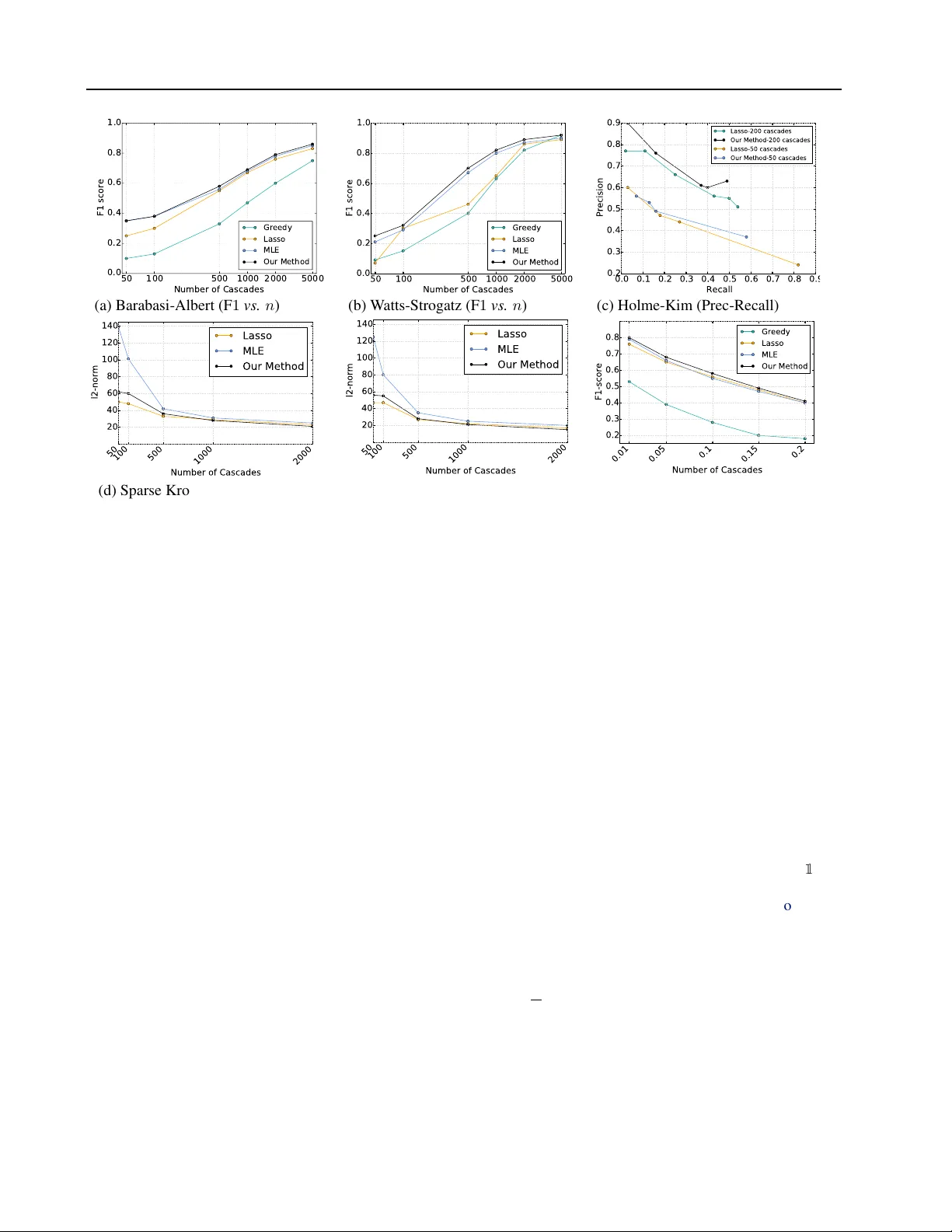
Inferring Graphs fr om Cascades: A Sparse Recov ery Framework Jean P ouget-Abadie J E A N P O U G E T A BA D I E @ G . H A RV A R D . E D U Harvard Uni versity Thibaut Horel T H O R E L @ S E A S . H A RV A R D . ED U Harvard Uni versity Abstract In the Network Inference problem, one seeks to recov er the edges of an unknown graph from the observations of cascades propagating ov er this graph. In this paper , we approach this prob- lem from the sparse reco very perspecti ve. W e introduce a general model of cascades, includ- ing the voter model and the independent cascade model, for which we provide the first algorithm which recov ers the graph’ s edges with high prob- ability and O ( s log m ) measurements where s is the maximum degree of the graph and m is the number of nodes. Furthermore, we show that our algorithm also recov ers the edge weights (the parameters of the dif fusion process) and is ro- bust in the context of approximate sparsity . Fi- nally we prov e an almost matching lower bound of Ω( s log m s ) and validate our approach empiri- cally on synthetic graphs. 1. Introduction Graphs hav e been extensiv ely studied for their propaga- tiv e abilities: connectivity , routing, gossip algorithms, etc. A diffusion process taking place ov er a graph provides valuable information about the presence and weights of its edges. Influence cascades are a specific type of diffusion processes in which a particular infectious beha vior spreads ov er the nodes of the graph. By only observing the “in- fection times” of the nodes in the graph, one might hope to recov er the underlying graph and the parameters of the cascade model. This problem is known in the literature as the Network Infer ence pr oblem . More precisely , solving the Network Inference problem in volves designing an algorithm taking as input a set of Pr oceedings of the 32 nd International Conference on Machine Learning , Lille, France, 2015. JMLR: W&CP volume 37. Copy- right 2015 by the author(s). observed cascades (realisations of the diffusion process) and recovers with high probability a large fraction of the graph’ s edges. The goal is then to understand the relation- ship between the number of observations, the probability of success, and the accuracy of the reconstruction. The Network Inference problem can be decomposed and analyzed “node-by-node”. Thus, we will focus on a sin- gle node of degree s and discuss how to identify its par- ents among the m nodes of the graph. Prior work has shown that the required number of observed cascades is O ( poly ( s ) log m ) ( Netrapalli & Sanghavi , 2012 ; Abrahao et al. , 2013 ). A more recent line of research ( Daneshmand et al. , 2014 ) has focused on applying adv ances in sparse recov ery to the network inference problem. Indeed, the graph can be in- terpreted as a “sparse signal” measured through influence cascades and then recovered. The challenge is that influ- ence cascade models typically lead to non-linear in verse problems and the measurements (the state of the nodes at different time steps) are usually correlated. The sparse re- cov ery literature suggests that Ω( s log m s ) cascade obser- vations should be sufficient to recover the graph ( Donoho , 2006 ; Candes & T ao , 2006 ). Howe ver , the best known up- per bound to this day is O ( s 2 log m ) ( Netrapalli & Sang- havi , 2012 ; Daneshmand et al. , 2014 ) The contributions of this paper are the follo wing: • we formulate the Graph Inference problem in the con- text of discrete-time influence cascades as a sparse re- cov ery problem for a specific type of Generalized Lin- ear Model. This formulation notably encompasses the well-studied Independent Cascade Model and V oter Model. • we gi ve an algorithm which recov ers the graph’ s edges using O ( s log m ) cascades. Furthermore, we show that our algorithm is also able to ef ficiently reco ver the edge weights (the parameters of the influence model) up to an additiv e error term, • we show that our algorithm is robust in cases where the signal to recov er is approximately s -sparse by Inferring Graphs from Cascades: A Sparse Recovery Framework proving guarantees in the stable r ecovery setting. • we pro vide an almost tight lower bound of Ω( s log m s ) observations required for sparse reco very . The organization of the paper is as follows: we conclude the introduction by a survey of the related work. In Sec- tion 2 we present our model of Generalized Linear Cas- cades and the associated sparse recov ery formulation. Its theoretical guarantees are presented for various recovery settings in Section 3 . The lower bound is presented in Sec- tion 4 . Finally , we conclude with e xperiments in Section 5 . Related W ork The study of edge prediction in graphs has been an active field of research for ov er a decade ( Liben-Nowell & Kleinber g , 2008 ; Leskovec et al. , 2007 ; Adar & Adamic , 2005 ). ( Gomez Rodriguez et al. , 2010 ) introduced the N E T I N F algorithm, which approx- imates the likelihood of cascades represented as a con- tinuous process. The algorithm was improved in later work ( Gomez-Rodriguez et al. , 2011 ), but is not known to hav e any theoretical guarantees beside empirical validation on synthetic networks. Netrapalli & Sanghavi ( 2012 ) stud- ied the discrete-time version of the independent cascade model and obtained the first O ( s 2 log m ) reco very guaran- tee on general networks. The algorithm is based on a like- lihood function similar to the one we propose, without the ` 1 -norm penalty . Their analysis depends on a corr elation decay assumption, which limits the number of new infec- tions at e very step. In this setting, they sho w a lo wer bound of the number of cascades needed for support recovery with constant probability of the order Ω( s log ( m/s )) . They also suggest a G R E E DY algorithm, which achie ves a O ( s log m ) guarantee in the case of tree graphs. The work of ( Abra- hao et al. , 2013 ) studies the same continuous-model frame- work as ( Gomez Rodriguez et al. , 2010 ) and obtains an O ( s 9 log 2 s log m ) support recov ery algorithm, without the corr elation decay assumption. ( Du et al. , 2013 ) propose a similar algorithm to ours for recovering the weights of the graph under a continuous-time independent cascade model, without proving theoretical guarantees. Closest to this work is a recent paper by Daneshmand et al. ( 2014 ), wherein the authors consider a ` 1 -regularized ob- jectiv e function. They adapt standard results from sparse recov ery to obtain a recovery bound of O ( s 3 log m ) under an irrepresentability condition ( Zhao & Y u , 2006 ). Under stronger assumptions, they match the ( Netrapalli & Sang- havi , 2012 ) bound of O ( s 2 log m ) , by exploiting similar properties of the con vex program’ s KKT conditions. In contrast, our work studies discrete-time diffusion processes including the Independent Cascade model under weaker as- sumptions. Furthermore, we analyze both the recov ery of the graph’ s edges and the estimation of the model’ s param- eters, and achiev e close to optimal bounds. The work of ( Du et al. , 2014 ) is slightly orthogonal to ours since they suggest learning the influence function, rather than the parameters of the network directly . 2. Model W e consider a graph G = ( V , E , Θ) , where Θ is a | V | × | V | matrix of parameters describing the edge weights of G . Intuitiv ely , Θ i,j captures the “influence” of node i on node j . Let m ≡ | V | . For each node j , let θ j be the j th column vector of Θ . A discrete-time Cascade model is a Markov process ov er a finite state space { 0 , 1 , . . . , K − 1 } V with the following properties: 1. Conditioned on the previous time step, the transition ev ents between two states in { 0 , 1 , . . . , K − 1 } for each i ∈ V are mutually independent across i ∈ V . 2. Of the K possible states, there exists a contagious state such that all transition probabilities of the Markov process can be expressed as a function of the graph parameters Θ and the set of “contagious nodes” at the previous time step. 3. The initial probability ov er { 0 , 1 , . . . , K − 1 } V is such that all nodes can eventually reach a contagious state with non-zero probability . The “contagious” nodes at t = 0 are called sour ce nodes . In other words, a cascade model describes a diffusion pro- cess where a set of contagious nodes “influence” other nodes in the graph to become contagious. An influence cas- cade is a realisation of this random process, i.e. the succes- siv e states of the nodes in graph G . Note that both the “sin- gle source” assumption made in ( Daneshmand et al. , 2014 ) and ( Abrahao et al. , 2013 ) as well as the “uniformly chosen source set” assumption made in ( Netrapalli & Sanghavi , 2012 ) verify condition 3. Also note that the multiple-source node assumption does not reduce to the single-source as- sumption, even under the assumption that cascades do not ov erlap. Imagining for e xample two cascades starting from two different nodes; since we do not observe which node propagated the contagion to which node, we cannot at- tribute an infected node to either cascade and treat the prob- lem as two independent cascades. In the context of Network Inference, ( Netrapalli & Sang- havi , 2012 ) focus on the well-kno wn discrete-time indepen- dent cascade model recalled below , which ( Abrahao et al. , 2013 ) and ( Daneshmand et al. , 2014 ) generalize to contin- uous time. W e extend the independent cascade model in a different direction by considering a more general class of transition probabilities while staying in the discrete-time setting. W e observe that despite their obvious differences, both the independent cascade and the voter models make Inferring Graphs from Cascades: A Sparse Recovery Framework the network inference problem similar to the standard gen- eralized linear model inference problem. In fact, we define a class of diffusion processes for which this is true: the Generalized Linear Cascade Models . The linear threshold model is a special case and is discussed in Section 6 . 2.1. Generalized Linear Cascade Models Let susceptible denote any state which can become conta- gious at the next time step with a non-zero probability . W e draw inspiration from generalized linear models to intro- duce Generalized Linear Cascades: Definition 1. Let X t be the indicator variable of “conta- gious nodes” at time step t . A generalized linear cascade model is a cascade model such that for each susceptible node j in state s at time step t , the pr obability of j becom- ing “contagious” at time step t + 1 conditioned on X t is a Bernoulli variable of parameter f ( θ j · X t ) : P ( X t +1 j = 1 | X t ) = f ( θ j · X t ) (1) wher e f : R → [0 , 1] In other words, each generalized linear cascade pro- vides, for each node j ∈ V a series of measurements ( X t , X t +1 j ) t ∈T j sampled from a generalized linear model. Note also that E [ X t +1 i | X t ] = f ( θ i · X t ) . As such, f can be interpreted as the inv erse link function of our general- ized linear cascade model. 2.2. Examples 2 . 2 . 1 . I N D E P E N D E N T C A S C A D E M O D E L In the independent cascade model, nodes can be either sus- ceptible, contagious or immune. At t = 0 , all source nodes are “contagious” and all remaining nodes are “susceptible”. At each time step t , for each edge ( i, j ) where j is suscep- tible and i is contagious, i attempts to infect j with proba- bility p i,j ∈ [0 , 1] ; the infection attempts are mutually in- dependent. If i succeeds, j will become contagious at time step t + 1 . Regardless of i ’ s success, node i will be immune at time t + 1 , such that nodes stay contagious for only one time step. The cascade process terminates when no conta- gious nodes remain. If we denote by X t the indicator v ariable of the set of con- tagious nodes at time step t , then if j is susceptible at time step t + 1 , we have: P  X t +1 j = 1 | X t  = 1 − m Y i =1 (1 − p i,j ) X t i . Defining Θ i,j ≡ log ( 1 1 − p i,j ) , this can be rewritten as: P  X t +1 j = 1 | X t  = 1 − m Y i =1 e − Θ i,j X t i (IC) = 1 − e − Θ j · X t Therefore, the independent cascade model is a Generalized Linear Cascade model with inv erse link function f : z 7→ 1 − e − z . Note that to write the Independent Cascade Model as a Generalized Linear Cascade Model, we had to intro- duce the change of variable Θ i,j = log( 1 1 − p i,j ) . The re- cov ery results in Section 3 pertain to the Θ j parameters. Fortunately , the follo wing lemma shows that the recovery error on Θ j is an upper bound on the error on the original p j parameters. Lemma 1. k ˆ θ − θ ∗ k 2 ≥ k ˆ p − p ∗ k 2 . 2 . 2 . 2 . T H E L I N E A R V OT E R M O D E L In the Linear V oter Model, nodes can be either r ed or blue . W ithout loss of generality , we can suppose that the blue nodes are contagious. The parameters of the graph are nor - malized such that ∀ i, P j Θ i,j = 1 . Each round, ev ery node j independently chooses one of its neighbors with probability Θ i,j and adopts their color . The cascades stops at a fixed horizon time T or if all nodes are of the same color . If we denote by X t the indicator variable of the set of blue nodes at time step t , then we hav e: P  X t +1 j = 1 | X t  = m X i =1 Θ i,j X t i = Θ j · X t (V) Thus, the linear voter model is a Generalized Linear Cas- cade model with in verse link function f : z 7→ z . 2 . 2 . 3 . D I S C R E T I Z ATI O N O F C O N T I N U O U S M O D E L Another motiv ation for the Generalized Linear Cascade model is that it captures the time-discretized formula- tion of the well-studied continuous-time independent cas- cade model with e xponential transmission function (CICE) of ( Gomez Rodriguez et al. , 2010 ; Abrahao et al. , 2013 ; Daneshmand et al. , 2014 ). Assume that the temporal reso- lution of the discretization is ε , i.e. all nodes whose (con- tinuous) infection time is within the interval [ kε, ( k + 1) ε ) are considered infected at (discrete) time step k . Let X k be the indicator vector of the set of nodes ‘infected’ before or during the k th time interv al. Note that contrary to the discrete-time independent cascade model, X k j = 1 = ⇒ X k +1 j = 1 , that is, there is no immune state and nodes remain contagious forev er . Let Exp ( p ) be an exponentially-distrib uted random vari- able of parameter p and let Θ i,j be the rate of transmis- Inferring Graphs from Cascades: A Sparse Recovery Framework Figure 1. Illustration of the sparse-recov ery approach. Our objec- tiv e is to recov er the unknown weight vector θ j for each node j . W e observe a Bernoulli realization whose parameters are gi ven by applying f to the matrix-vector product, where the measurement matrix encodes which nodes are “contagious” at each time step. sion along directed edge ( i, j ) in the CICE model. By the memoryless property of the exponential, if X k j 6 = 1 : P ( X k +1 j = 1 | X k ) = P ( min i ∈N ( j ) Exp (Θ i,j ) ≤  ) = P ( Exp ( m X i =1 Θ i,j X t i ) ≤  ) = 1 − e −  Θ j · X t Therefore, the  -discretized CICE-induced process is a Generalized Linear Cascade model with in verse link func- tion f : z 7→ 1 − e −  · z . 2 . 2 . 4 . L O G I S T I C C A S C A D E S “Logistic cascades” is the specific case where the in verse link function is gi ven by the logistic function f ( z ) = 1 / (1 + e − z + t ) . Intuitively , this captures the idea that there is a threshold t such that when the sum of the parameters of the infected parents of a node is larger than the threshold, the probability of getting infected is close to one. This is a smooth approximation of the hard threshold rule of the Linear Threshold Model ( Kempe et al. , 2003 ). As we will see later in the analysis, for logistic cascades, the graph in- ference problem becomes a linear in verse problem. 2.3. Maximum Likelihood Estimation Inferring the model parameter Θ from observed influence cascades is the central question of the present work. Recov- ering the edges in E from observed influence cascades is a well-identified problem known as the Network Inference problem. Ho wever , recovering the influence parameters is no less important. In this work we focus on recovering Θ , noting that the set of edges E can then be recovered through the following equi valence: ( i, j ) ∈ E ⇔ Θ i,j 6 = 0 Giv en observ ations ( x 1 , . . . , x n ) of a cascade model, we can reco ver Θ via Maximum Likelihood Estimation (MLE). Denoting by L the log-likelihood function, we con- sider the following ` 1 -regularized MLE problem: ˆ Θ ∈ argmax Θ 1 n L (Θ | x 1 , . . . , x n ) − λ k Θ k 1 where λ is the regularization factor which helps prevent ov erfitting and controls the sparsity of the solution. The generalized linear cascade model is decomposable in the following sense: gi ven Definition 1 , the log-likelihood can be written as the sum of m terms, each term i ∈ { 1 , . . . , m } only depending on θ i . Since this is equally true for k Θ k 1 , each column θ i of Θ can be estimated by a separate optimization program: ˆ θ i ∈ argmax θ L i ( θ i | x 1 , . . . , x n ) − λ k θ i k 1 (2) where we denote by T i the time steps at which node i is susceptible and: L i ( θ i | x 1 , . . . , x n ) = 1 |T i | X t ∈T i x t +1 i log f ( θ i · x t ) + (1 − x t +1 i ) log  1 − f ( θ i · x t )  In the case of the voter model, the measurements include all time steps until we reach the time horizon T or the graph coalesces to a single state. For the independent cascade model, the measurements include all time steps until node i becomes contagious, after which its behavior is determin- istic. Contrary to prior work, our results depend on the number of measurements and not the number of cascades. Regularity assumptions T o solve program ( 2 ) effi- ciently , we would like it to be conv ex. A sufficient condi- tion is to assume that L i is concave, which is the case if f and (1 − f ) are both log-conca ve. Remember that a twice- differentiable function f is log-concav e iff. f 00 f ≤ f 0 2 . It is easy to verify this property for f and (1 − f ) in the Independent Cascade Model and V oter Model. Furthermore, the data-dependent bounds in Section 3.1 will require the following regularity assumption on the inv erse link function f : there exists α ∈ (0 , 1) such that max  | (log f ) 0 ( z x ) | , | (log (1 − f )) 0 ( z x ) |  ≤ 1 α (LF) for all z x ≡ θ ∗ · x such that f ( z x ) / ∈ { 0 , 1 } . In the voter model, f 0 ( z ) f ( z ) = 1 z and f 0 ( z ) (1 − f )( z ) = 1 1 − z . Hence (LF) will hold as soon as α ≤ Θ i,j ≤ 1 − α for all ( i, j ) ∈ E which is always satisfied for some α for non-isolated nodes. In the Independent Cascade Model, f 0 ( z ) f ( z ) = 1 e z − 1 and f 0 ( z ) (1 − f )( z ) = 1 . Hence (LF) holds as soon as p i,j ≥ α for all ( i, j ) ∈ E which is always satisfied for some α ∈ (0 , 1) . For the data-independent bound of Proposition 1 , we will require the following additional re gularity assumption: max  | (log f ) 00 ( z x ) | , | (log (1 − f )) 00 ( z x ) |  ≤ 1 α (LF2) Inferring Graphs from Cascades: A Sparse Recovery Framework for some α ∈ (0 , 1) and for all z x ≡ θ ∗ · x such that f ( z x ) / ∈ { 0 , 1 } . It is again easy to see that this condition is verified for the Independent Cascade Model and the V oter model for the same α ∈ (0 , 1) . Con vex constraints The voter model is only defined when Θ i,j ∈ (0 , 1) for all ( i, j ) ∈ E . Similarly the in- dependent cascade model is only defined when Θ i,j > 0 . Because the likelihood function L i is equal to −∞ when the parameters are outside of the domain of definition of the models, these contraints do not need to appear explic- itly in the optimization program. In the specific case of the voter model, the constraint P j Θ i,j = 1 will not necessarily be verified by the es- timator obtained in ( 2 ). In some applications, the exper- imenter might not need this constraint to be verified, in which case the results in Section 3 still giv e a bound on the recovery error . If this constraint needs to be satisfied, then by Lagrangian duality , there exists a λ ∈ R such that adding λ  P j θ j − 1  to the objectiv e function of ( 2 ) en- forces the constraint. Then, it suffices to apply the results of Section 3 to the augmented objective to obtain the same recov ery guarantees. Note that the added term is linear and will easily satisfy all the required regularity assumptions. 3. Results In this section, we apply the sparse recovery framew ork to analyze under which assumptions our program ( 2 ) recovers the true parameter θ i of the cascade model. Furthermore, if we can estimate θ i to a sufficiently good accuracy , it is then possible to reco ver the support of θ i by simple thresh- olding, which provides a solution to the standard Network Inference problem. W e will first giv e results in the exactly sparse setting in which θ i has a support of size exactly s . W e will then relax this sparsity constraint and giv e results in the stable r ecov- ery setting where θ i is approximately s -sparse. As mentioned in Section 2.3 , the maximum likelihood es- timation program is decomposable. W e will henceforth fo- cus on a single node i ∈ V and omit the subscript i in the notations when there is no ambiguity . The recovery prob- lem is now the one of estimating a single vector θ ∗ from a set T of observations. W e will write n ≡ |T | . 3.1. Main Theorem In this section, we analyze the case where θ ∗ is exactly sparse. W e write S ≡ supp ( θ ∗ ) and s = | S | . Recall, that θ i is the vector of weights for all edges directed at the node we are solving for . In other words, S is the set of all nodes susceptible to influence node i , also referred to as its parents. Our main theorem will rely on the no w standard r estricted eig envalue condition introduced by ( Bickel et al. , 2009a ). Definition 2. Let Σ ∈ S m ( R ) be a real symmetric matrix and S be a subset of { 1 , . . . , m } . Defining C ( S ) ≡ { X ∈ R m : k X S c k 1 ≤ 3 k X S k 1 } . W e say that Σ satisfies the ( S, γ ) - restricted eigen value condition if f: ∀ X ∈ C ( S ) , X T Σ X ≥ γ k X k 2 2 (RE) A discussion of the ( S, γ ) - (RE) assumption in the context of generalized linear cascade models can be found in Sec- tion 3.3 . In our setting we require that the (RE) -condition holds for the Hessian of the log-likelihood function L : it es- sentially captures the fact that the binary vectors of the set of acti ve nodes ( i.e the measurements) are not too collinear . Theorem 1. Assume the Hessian ∇ 2 L ( θ ∗ ) satisfies the ( S, γ ) - (RE) for some γ > 0 and that (LF) holds for some α > 0 . F or any δ ∈ (0 , 1) , let ˆ θ be the solution of ( 2 ) with λ ≡ 2 q log m αn 1 − δ , then: k ˆ θ − θ ∗ k 2 ≤ 6 γ r s log m αn 1 − δ w .p. 1 − 1 e n δ log m (3) Note that we have expressed the con ver gence rate in the number of measurements n , which is different from the number of cascades. For example, in the case of the voter model with horizon time T and for N cascades, we can expect a number of measurements proportional to N × T . Theorem 1 is a consequence of Theorem 1 in ( Negahban et al. , 2012 ) which gives a bound on the con vergence rate of regularized estimators. W e state their theorem in the context of ` 1 regularization in Lemma 2 . Lemma 2. Let C ( S ) ≡ { ∆ ∈ R m | k ∆ S k 1 ≤ 3 k ∆ S c k 1 } . Suppose that: ∀ ∆ ∈ C ( S ) , L ( θ ∗ + ∆) − L ( θ ∗ ) − ∇L ( θ ∗ ) · ∆ ≥ κ L k ∆ k 2 2 − τ 2 L ( θ ∗ ) (4) for some κ L > 0 and function τ L . F inally suppose that λ ≥ 2 k∇L ( θ ∗ ) k ∞ , then if ˆ θ λ is the solution of ( 2 ) : k ˆ θ λ − θ ∗ k 2 2 ≤ 9 λ 2 s κ L + λ κ 2 L 2 τ 2 L ( θ ∗ ) T o prove Theorem 1 , we apply Lemma 2 with τ L = 0 . Since L is twice differentiable and con vex, assumption ( 4 ) with κ L = γ 2 is implied by the (RE)-condition. For a good con vergence rate, we must find the smallest possible value of λ such that λ ≥ 2 k∇L θ ∗ k ∞ . The upper bound on the ` ∞ norm of ∇L ( θ ∗ ) is gi ven by Lemma 3 . Inferring Graphs from Cascades: A Sparse Recovery Framework Lemma 3. Assume (LF) holds for some α > 0 . F or any δ ∈ (0 , 1) : k∇L ( θ ∗ ) k ∞ ≤ 2 r log m αn 1 − δ w .p. 1 − 1 e n δ log m The proof of Lemma 3 relies crucially on Azuma- Hoeffding’ s inequality , which allows us to handle corre- lated observations. This departs from the usual assump- tions made in sparse recovery settings, that the measure- ments are independent from one another . W e now show how to use Theorem 1 to recov er the support of θ ∗ , that is, to solve the Network Inference problem. Corollary 1. Under the same assumptions as Theor em 1 , let ˆ S η ≡ { j ∈ { 1 , . . . , m } : ˆ θ j > η } for η > 0 . F or 0 <  < η , let S ∗ η +  ≡ { i ∈ { 1 , . . . , m } : θ ∗ i > η +  } be the set of all true ‘str ong’ par ents. Suppose the number of measur ements verifies: n > 9 s log m αγ 2  2 . Then with pr obability 1 − 1 m , S ∗ η +  ⊆ ˆ S η ⊆ S ∗ . In other words we reco ver all ‘str ong’ par ents and no ‘false’ parents. Assuming we know a lo wer bound α on Θ i,j , Corollary 1 can be applied to the Network Inference problem in the fol- lowing manner: pick  = η 2 and η = α 3 , then S ∗ η +  = S provided that n = Ω  s log m α 3 γ 2  . That is, the support of θ ∗ can be found by thresholding ˆ θ to the level η . 3.2. Appr oximate Sparsity In practice, exact sparsity is rarely verified. For social net- works in particular , it is more realistic to assume that each node has few “strong” parents’ and many “weak” parents. In other words, even if θ ∗ is not exactly s -sparse, it can be well approximated by s -sparse vectors. Rather than obtaining an impossibility result, we show that the bounds obtained in Section 3.1 degrade gracefully in this setting. Formally , let θ ∗ b s c ∈ argmin k θ k 0 ≤ s k θ − θ ∗ k 1 be the best s -approximation to θ ∗ . Then we pay a cost pro- portional to k θ ∗ − θ ∗ b s c k 1 for recov ering the weights of non- exactly sparse vectors. This cost is simply the “tail” of θ ∗ : the sum of the m − s smallest coordinates of θ ∗ . W e re- cov er the results of Section 3.1 in the limit of exact spar- sity . These results are formalized in the follo wing theorem, which is also a consequence of Theorem 1 in ( Negahban et al. , 2012 ). Theorem 2. Suppose the (RE) assumption holds for the Hessian ∇ 2 f ( θ ∗ ) and τ L ( θ ∗ ) = κ 2 log m n k θ ∗ k 1 on the fol- lowing set: C 0 ≡{ X ∈ R p : k X S c k 1 ≤ 3 k X S k 1 + 4 k θ ∗ − θ ∗ b s c k 1 } ∩ {k X k 1 ≤ 1 } If the number of measurements n ≥ 64 κ 2 γ s log m , then by solving ( 2 ) for λ ≡ 2 q log m αn 1 − δ we have: k ˆ θ − θ ∗ k 2 ≤ 3 γ r s log m αn 1 − δ + 4 4 s s log m γ 4 αn 1 − δ k θ ∗ − θ ∗ b s c k 1 As in Corollary 1 , an edge recov ery guarantee can be de- riv ed from Theorem 2 in the case of approximate sparsity . 3.3. Restricted Eigen value Condition There exists a large class of suf ficient conditions under which sparse recovery is achiev able in the context of regu- larized estimation ( van de Geer & Bühlmann , 2009 ). The restricted eigen value condition, introduced in ( Bickel et al. , 2009b ), is one of the weakest such assumption. It can be interpreted as a restricted form of non-degenerac y . Since we apply it to the Hessian of the log-likelihood function ∇ 2 L ( θ ) , it essentially reduces to a form of restricted strong con vexity , that Lemma 2 ultimately relies on. Observe that the Hessian of L can be seen as a re-weighted Gram matrix of the observ ations: ∇ 2 L ( θ ∗ ) = 1 |T | X t ∈T x t ( x t ) T  x t +1 i f 00 f − f 0 2 f 2 ( θ ∗ · x t ) − (1 − x t +1 i ) f 00 (1 − f ) + f 0 2 (1 − f ) 2 ( θ ∗ · x t )  If f and (1 − f ) are c -strictly log-conv ex for c > 0 , then min ((log f ) 00 , (log (1 − f )) 00 ) ≥ c . This implies that the ( S, γ ) -( RE ) condition in Theorem 1 and Theorem 2 re- duces to a condition on the Gram matrix of the observations X T X = 1 |T | P t ∈T x t ( x t ) T for γ 0 ≡ γ · c . (RE) with high probability The Generalized Linear Cascade model yields a probability distribution over the ob- served sets of infected nodes ( x t ) t ∈T . It is then natural to ask whether the restricted eigen value condition is likely to occur under this probabilistic model. Sev eral recent papers show that large classes of correlated designs obey the re- stricted eigen value property with high probability ( Raskutti et al. , 2010 ; Rudelson & Zhou , 2013 ). The (RE) -condition has the following concentration prop- erty: if it holds for the expected Hessian matrix E [ ∇ 2 L ( θ ∗ )] , then it holds for the finite sample Hessian ma- trix ∇ 2 L ( θ ∗ ) with high probability . Therefore, under an assumption which only in volv es the probabilistic model and not the actual observations, we can obtain the same conclusion as in Theorem 1 : Proposition 1. Suppose E [ ∇ 2 L ( θ ∗ )] verifies the ( S, γ ) - (RE) condition and assume (LF) and (LF2) . F or δ > 0 , if n 1 − δ ≥ 1 28 γ α s 2 log m , then ∇ 2 L ( θ ∗ ) verifies the ( S, γ 2 ) - (RE) condition, w .p ≥ 1 − e − n δ log m . Inferring Graphs from Cascades: A Sparse Recovery Framework Observe that the number of measurements required in Proposition 1 is now quadratic in s . If we only keep the first measurement from each cascade, which are in- dependent, we can apply Theorem 1.8 from ( Rudelson & Zhou , 2013 ), lowering the number of required cascades to s log m log 3 ( s log m ) . If f and (1 − f ) are strictly log-conv ex, then the previous observations show that the quantity E [ ∇ 2 L ( θ ∗ )] in Propo- sition 1 can be replaced by the expected Gram matrix : A ≡ E [ X T X ] . This matrix A has a natural interpretation: the entry a i,j is the probability that node i and node j are infected at the same time during a cascade. In particular , the diagonal term a i,i is simply the probability that node i is infected during a cascade. 4. A Lower Bound In ( Netrapalli & Sangha vi , 2012 ), the authors explicitate a lower bound of Ω( s log m s ) on the number of cascades necessary to achiev e good support recovery with constant probability under a corr elation decay assumption. In this section, we will consider the stable sparse recovery set- ting of Section 3.2 . Our goal is to obtain an information- theoretic lo wer bound on the number of measurements nec- essary to approximately recover the parameter θ ∗ of a cas- cade model from observ ed cascades. Similar lower bounds were obtained for sparse linear in verse problems in ( Price & W oodruff , 2011 ; 2012 ; Ba et al. , 2011 ). Theorem 3. Let us consider a cascade model of the form ( 1 ) and a recovery algorithm A which takes as input n ran- dom cascade measurements and outputs ˆ θ such that with pr obability δ > 1 2 (over the measur ements): k ˆ θ − θ ∗ k 2 ≤ C min k θ k 0 ≤ s k θ − θ ∗ k 2 (5) wher e θ ∗ is the true parameter of the cascade model. Then n = Ω( s log m s / log C ) . This theorem should be contrasted with Theorem 2 : up to an additiv e s log s factor , the number of measurements re- quired by our algorithm is tight. The proof of Theorem 3 follows an approach similar to ( Price & W oodruff , 2012 ). W e present a sketch of the proof in the Appendix and refer the reader to their paper for more details. 5. Experiments In this section, we validate empirically the results and as- sumptions of Section 3 for varying levels of sparsity and different initializations of parameters ( n , m , λ , p init ), where p init is the initial probability of a node being a source node. W e compare our algorithm to two different state-of-the-art algorithms: G R E E DY and M L E from ( Netrapalli & Sang- havi , 2012 ). As an extra benchmark, we also introduce a new algorithm L A S S O , which approximates our S PA R S E M L E algorithm. Experimental setup W e ev aluate the performance of the algorithms on synthetic graphs, chosen for their similarity to real social networks. W e therefore consider a W atts- Strogatz graph ( 300 nodes, 4500 edges) ( W atts & Stro- gatz , 1998 ), a Barabasi-Albert graph ( 300 nodes, 16200 edges) ( Albert & Barabási , 2001 ), a Holme-Kim power law graph ( 200 nodes, 9772 edges) ( Holme & Kim , 2002 ), and the recently introduced Kronecker graph ( 256 nodes, 10000 edges) ( Leskov ec et al. , 2010 ). Undirected graphs are con- verted to directed graphs by doubling the edges. For every reported data point, we sample edge weights and generate n cascades from the (IC) model for n ∈ { 100 , 500 , 1000 , 2000 , 5000 } . W e compare for each algo- rithm the estimated graph ˆ G with G . The initial probability of a node being a source is fixed to 0 . 05 , i.e. an average of 15 nodes source nodes per cascades for all e xperiments, e x- cept for Figure (f). All edge weights are chosen uniformly in the interval [0 . 2 , 0 . 7] , except when testing for approxi- mately sparse graphs (see paragraph on robustness). Ad- justing for the variance of our experiments, all data points are reported with at most a ± 1 error margin. The param- eter λ is chosen to be of the order O ( p log m/ ( αn )) . W e report our results as a function of the number of cascades and not the number of measur ements : in practice, very fe w cascades hav e depth greater than 3. Benchmarks W e compare our S PA RS E M L E algorithm to 3 benchmarks: G R E E DY and M L E from ( Netrapalli & Sanghavi , 2012 ) and L A S S O . The M L E algorithm is a maximum-likelihood estimator without ` 1 -norm penaliza- tion. G R E E DY is an iterativ e algorithm. W e introduced the L A S S O algorithm in our experiments to achie ve f aster com- putation time: ˆ θ i ∈ arg min θ X t ∈T | f ( θ i · x t ) − x t +1 i | 2 + λ k θ i k 1 L A S S O has the merit of being both easier and faster to opti- mize numerically than the other con ve x-optimization based algorithms. It approximates the S PA R S E M L E algorithm by making the assumption that the observ ations x t +1 i are of the form: x t +1 i = f ( θ i · x t ) +  , where  is random white noise. This is not valid in theory since  depends on f ( θ i · x t ) , howe ver the approximation is v alidated in practice. W e did not benchmark against other known algorithms ( N E T R AT E ( Gomez-Rodriguez et al. , 2011 ) and FI R S T E D G E ( Abrahao et al. , 2013 )) due to the discrete-time as- sumption. These algorithms also suppose a single-source model, whereas S PA R S E M L E , M L E , and G R E E D Y do not. Learning the graph in the case of a multi-source cascade Inferring Graphs from Cascades: A Sparse Recovery Framework 50 100 500 1000 2000 5000 Number of Cascades 0.0 0.2 0.4 0.6 0.8 1.0 F1 score Greedy Lasso MLE Our Method (a) Barabasi-Albert (F 1 vs. n ) (b) W atts-Strogatz (F 1 vs. n ) (c) Holme-Kim (Prec-Recall) (d) Sparse Kronecker ( ` 2 -norm vs. n ) (e) Non-sparse Kronecker ( ` 2 -norm vs. n ) (f) W atts-Strogatz (F 1 vs. p init ) Figure 2. Figures (a) and (b) report the F 1 -score in log scale for 2 graphs as a function of the number of cascades n : (a) Barabasi-Albert graph, 300 nodes, 16200 edges. (b) W atts-Strogatz graph, 300 nodes, 4500 edges. Figure (c) plots the Precision-Recall curve for various values of λ for a Holme-Kim graph ( 200 nodes, 9772 edges). Figures (d) and (e) report the ` 2 -norm k ˆ Θ − Θ k 2 for a Kronecker graph which is: (d) exactly sparse (e) non-exactly sparse, as a function of the number of cascades n . Figure (f) plots the F 1 -score for the W atts-Strogatz graph as a function of p init . model is harder (see Figure 2 (f)) but more realistic, since we rarely hav e access to “patient 0” in practice. Graph Estimation In the case of the L A S S O , M L E and S PA RS E M L E algorithms, we construct the edges of ˆ G : ∪ j ∈ V { ( i, j ) : Θ ij > 0 . 1 } , i.e by thresholding. Finally , we report the F1-score = 2 precision · recall / ( precision + recall ) , which considers (1) the number of true edges recov ered by the algorithm over the total number of edges returned by the algorithm ( precision ) and (2) the number of true edges recov ered by the algorithm over the total number of edges it should have recovered ( recall ). Over all experiments, S PA RS E M L E achieves higher rates of precision, recall, and F1-score. Interestingly , both M L E and S PA R S E M L E per- form exceptionally well on the W atts-Strogatz graph. Quantifying rob ustness The previous experiments only considered graphs with strong edges. T o test the algorithms in the approximately sparse case, we add sparse edges to the pre vious graphs according to a bernoulli v ariable of pa- rameter 1 / 3 for e very non-edge, and drawing a weight uni- formly from [0 , 0 . 1] . The non-sparse case is compared to the sparse case in Figure 2 (d)–(e) for the ` 2 norm show- ing that both the L A S S O , followed by S PA R S E M L E are the most robust to noise. 6. Future W ork Solving the Graph Inference problem with sparse recovery techniques opens new venues for future work. Firstly , the sparse recov ery literature has already studied regulariza- tion patterns beyond the ` 1 -norm, notably the thresholded and adapti ve lasso ( v an de Geer et al. , 2011 ; Zou , 2006 ). Another goal would be to obtain confidence intervals for our estimator , similarly to what has been obtained for the Lasso in the recent series of papers ( Jav anmard & Monta- nari , 2014 ; Zhang & Zhang , 2014 ). Finally , the linear threshold model is a commonly stud- ied diffusion process and can also be cast as a gener al- ized linear cascade with inv erse link function z 7→ 1 z > 0 : X t +1 j = sign ( θ j · X t − t j ) . This model therefore falls into the 1-bit compressed sensing frame work ( Boufounos & Baraniuk , 2008 ). Several recent papers study the the- oretical guarantees obtained for 1-bit compressed sensing with specific measurements ( Gupta et al. , 2010 ; Plan & V ershynin , 2014 ). Whilst the y obtained bounds of the order O ( s log m s ), no current theory exists for recovering positiv e bounded signals from binary measurememts. This research direction may provide the first clues to solve the “adaptiv e learning” problem: if we are allowed to adaptively choose the source nodes at the beginning of each cascade, how much can we improv e the current results? Inferring Graphs from Cascades: A Sparse Recovery Framework Acknowledgments W e would like to thank Y aron Singer , David P arkes, Jelani Nelson, Edoardo Airoldi and Or Shef fet for helpful discus- sions. W e are also grateful to the anonymous revie wers for their insightful feedback and suggestions. References Abrahao, Bruno D., Chierichetti, Flavio, Kleinberg, Robert, and Panconesi, Alessandro. Trace complexity of network inference. In The 19th A CM SIGKDD Inter- national Confer ence on Knowledge Discovery and Data Mining, KDD 2013, Chicago, IL, USA, August 11-14, 2013 , pp. 491–499, 2013. Adar , Eytan and Adamic, Lada A. T racking information epidemics in blogspace. In 2005 IEEE / WIC / ACM In- ternational Conference on W eb Intelligence (WI 2005), 19-22 September 2005, Compiegne , F rance , pp. 207– 214, 2005. Albert, Réka and Barabási, Albert-László. Statisti- cal mechanics of complex networks. CoRR , cond- mat/0106096, 2001. Ba, Khanh Do, Indyk, Piotr , Price, Eric, and W oodruff, David P . Lower bounds for sparse recovery . CoRR , abs/1106.0365, 2011. Bickel, Peter J, Ritov , Y a’acov , and Tsybakov , Alexan- dre B. Simultaneous analysis of lasso and dantzig se- lector . The Annals of Statistics , pp. 1705–1732, 2009a. Bickel, Peter J., Ritov , Y a’acov , and Tsybako v , Alexan- dre B. Simultaneous analysis of lasso and dantzig se- lector . Ann. Statist. , 37(4):1705–1732, 08 2009b. Boufounos, Petros and Baraniuk, Richard G. 1-bit com- pressiv e sensing. In 42nd Annual Confer ence on Infor- mation Sciences and Systems, CISS 2008, Princeton, NJ , USA, 19-21 Mar ch 2008 , pp. 16–21, 2008. Candes, Emmanuel J and T ao, T erence. Near-optimal sig- nal recov ery from random projections: Univ ersal encod- ing strategies? Information Theory , IEEE T ransactions on , 52(12):5406–5425, 2006. Daneshmand, Hadi, Gomez-Rodriguez, Manuel, Song, Le, and Schölkopf, Bernhard. Estimating diffusion network structures: Recov ery conditions, sample complexity & soft-thresholding algorithm. In Pr oceedings of the 31th International Conference on Machine Learning, ICML 2014, Beijing, China, 21-26 June 2014 , pp. 793–801, 2014. Donoho, David L. Compressed sensing. Information The- ory , IEEE T ransactions on , 52(4):1289–1306, 2006. Du, Nan, Song, Le, W oo, Hyenkyun, and Zha, Hongyuan. Uncov er topic-sensitiv e information diffusion networks. In Pr oceedings of the Sixteenth International Confer - ence on Artificial Intelligence and Statistics , pp. 229– 237, 2013. Du, Nan, Liang, Y ingyu, Balcan, Maria, and Song, Le. In- fluence function learning in information dif fusion net- works. In Proceedings of the 31st International Confer- ence on Machine Learning (ICML-14) , pp. 2016–2024, 2014. Gomez Rodriguez, Manuel, Leskov ec, Jure, and Krause, Andreas. Inferring networks of diffusion and influence. In Proceedings of the 16th ACM SIGKDD International Confer ence on Knowledge Discovery and Data Mining , KDD ’10, pp. 1019–1028, New Y ork, NY , USA, 2010. A CM. ISBN 978-1-4503-0055-1. Gomez-Rodriguez, Manuel, Balduzzi, David, and Schölkopf, Bernhard. Uncovering the temporal dy- namics of diffusion networks. CoRR , abs/1105.0697, 2011. Gupta, Ankit, Nowak, Robert, and Recht, Benjamin. Sam- ple complexity for 1-bit compressed sensing and sparse classification. In IEEE International Symposium on In- formation Theory , ISIT 2010, J une 13-18, 2010, Austin, T exas, USA, Pr oceedings , pp. 1553–1557, 2010. Holme, Petter and Kim, Beom Jun. Growing scale-free networks with tunable clustering. Physical r eview E , 65: 026–107, 2002. Jav anmard, Adel and Montanari, Andrea. Confidence in- tervals and hypothesis testing for high-dimensional re- gression. The Journal of Machine Learning Resear ch , 15(1):2869–2909, 2014. Kempe, David, Kleinber g, Jon M., and T ardos, Év a. Maxi- mizing the spread of influence through a social network. In Pr oceedings of the Ninth A CM SIGKDD International Confer ence on Knowledge Discovery and Data Mining, W ashington, DC, USA, August 24 - 27, 2003 , pp. 137– 146, 2003. Leskov ec, Jure, McGlohon, Mary , Faloutsos, Christos, Glance, Natalie S., and Hurst, Matthew . Patterns of cas- cading behavior in large blog graphs. In Proceedings of the Seventh SIAM International Confer ence on Data Mining, April 26-28, 2007, Minneapolis, Minnesota, USA , pp. 551–556, 2007. Leskov ec, Jure, Chakrabarti, Deepayan, Kleinberg, J on M., Faloutsos, Christos, and Ghahramani, Zoubin. Kro- necker graphs: An approach to modeling netw orks. Journal of Machine Learning Resear ch , 11:985–1042, 2010. Inferring Graphs from Cascades: A Sparse Recovery Framework Liben-Nowell, David and Kleinberg, Jon. Tracing infor- mation flow on a global scale using Internet chain-letter data. Pr oceedings of the National Academy of Sciences , 105(12):4633–4638, 2008. Negahban, Sahand N., Ravikumar , Pradeep, Wrainwright, Martin J., and Y u, Bin. A unified frame work for high- dimensional analysis of m-estimators with decompos- able regularizers. Statistical Science , 27(4):538–557, December 2012. Netrapalli, Praneeth and Sangha vi, Sujay . Learning the graph of epidemic cascades. SIGMETRICS P erform. Eval. Rev . , 40(1), June 2012. ISSN 0163-5999. Plan, Y aniv and V ershynin, Roman. Dimension reduction by random hyperplane tessellations. Discr ete & Compu- tational Geometry , 51(2):438–461, 2014. Price, Eric and W oodruff, David P . (1 + eps)-approximate sparse recovery . In Ostrovsky , Rafail (ed.), IEEE 52nd Annual Symposium on F oundations of Computer Sci- ence, FOCS 2011, P alm Springs, CA, USA, October 22- 25, 2011 , pp. 295–304. IEEE Computer Society , 2011. ISBN 978-1-4577-1843-4. Price, Eric and W oodruff, David P . Applications of the shannon-hartley theorem to data streams and sparse re- cov ery . In Pr oceedings of the 2012 IEEE International Symposium on Information Theory , ISIT 2012, Cam- bridge, MA, USA, J uly 1-6, 2012 , pp. 2446–2450. IEEE, 2012. ISBN 978-1-4673-2580-6. Raskutti, Garvesh, W ainwright, Martin J., and Y u, Bin. Re- stricted eigen value properties for correlated gaussian de- signs. Journal of Machine Learning Resear ch , 11:2241– 2259, 2010. Rudelson, Mark and Zhou, Shuheng. Reconstruction from anisotropic random measurements. IEEE T ransactions on Information Theory , 59(6):3434–3447, 2013. van de Geer , Sara, Bühlmann, Peter , and Zhou, Shuheng. The adapti ve and the thresholded lasso for potentially misspecified models (and a lower bound for the lasso). Electr on. J. Statist. , 5:688–749, 2011. van de Geer, Sara A. and Bühlmann, Peter . On the condi- tions used to prov e oracle results for the lasso. Electron. J. Statist. , 3:1360–1392, 2009. W atts, Duncan J. and Strogatz, Stev en H. Collective dy- namics of ‘small-world’ networks. Natur e , 393(6684): 440–442, 1998. Zhang, Cun-Hui and Zhang, Stephanie S. Confidence in- tervals for low dimensional parameters in high dimen- sional linear models. J ournal of the Royal Statistical Society: Series B (Statistical Methodology) , 76(1):217– 242, 2014. Zhao, Peng and Y u, Bin. On model selection consistency of lasso. J. Mach. Learn. Res. , 7:2541–2563, December 2006. ISSN 1532-4435. Zou, Hui. The adaptiv e lasso and its oracle properties. Journal of the American Statistical Association , 101 (476):1418–1429, 2006. Inferring Graphs from Cascades: A Sparse Recovery Framework 7. A ppendix In this appendix, we provide the missing proofs of Sec- tion 3 and Section 4 . W e also show additional experiments on the running time of our recov ery algorithm which could not fit in the main part of the paper . 7.1. Proofs of Section 3 Pr oof of Lemma 1 . Using the inequality ∀ x > 0 , log x ≥ 1 − 1 x , we hav e | log ( 1 1 − p ) − log ( 1 1 − p 0 ) | ≥ max(1 − 1 − p 1 − p 0 , 1 − 1 − p 0 1 − p ) ≥ max( p − p 0 , p 0 − p ) . Pr oof of Lemma 3 . The gradient of L is giv en by: ∇L ( θ ∗ ) = 1 |T | X t ∈T x t  x t +1 i f 0 f ( θ ∗ · x t ) − (1 − x t +1 i ) f 0 1 − f ( θ ∗ · x t )  Let ∂ j L ( θ ) be the j -th coordinate of ∇L ( θ ∗ ) . Writing ∂ j L ( θ ∗ ) = 1 |T | P t ∈T Y t and since E [ x t +1 i | x t ] = f ( θ ∗ · x t ) , we have that E [ Y t +1 | Y t ] = 0 . Hence Z t = P t k =1 Y k is a martingale. Using assumption (LF), we have almost surely | Z t +1 − Z t | ≤ 1 α and we can apply Azuma’ s inequality to Z t : P  | Z T | ≥ λ  ≤ 2 exp  − λ 2 α 2 n  Applying a union bound to hav e the previous inequality hold for all coordinates of ∇L ( θ ) implies: P  k∇L ( θ ∗ ) k ∞ ≥ λ  ≤ 2 m exp  − λ 2 nα 2  Choosing λ ≡ 2 q log m αn 1 − δ concludes the proof. Pr oof of Cor ollary 1 . By choosing δ = 0 , if n > 9 s log m αγ 2  2 , then k ˆ θ − θ ∗ k 2 <  < η with probability 1 − 1 m . If θ ∗ i = 0 and ˆ θ > η , then k ˆ θ − θ ∗ k 2 ≥ | ˆ θ i − θ ∗ i | > η , which is a contradiction. Therefore we get no false positiv es. If θ ∗ i > η +  , then | ˆ θ i − θ ∗ i | <  = ⇒ θ j > η and we get all strong parents. (RE) with high probability W e no w prove Proposi- tion 1 . The proof mostly relies on sho wing that the Hessian of likelihood function L is sufficiently well concentrated around its expectation. Pr oof. Writing H ≡ ∇ 2 L ( θ ∗ ) , if ∀ ∆ ∈ C ( S ) , k E [ H ] − H ] k ∞ ≤ λ and E [ H ] verifies the ( S, γ ) -(RE) condition then: ∀ ∆ ∈ C ( S ) , ∆ H ∆ ≥ ∆ E [ H ]∆(1 − 32 sλ/γ ) (6) Indeed, | ∆( H − E [ H ])∆ | ≤ 2 λ k ∆ k 2 1 ≤ 2 λ (4 √ s k ∆ s k 2 ) 2 . Writing ∂ 2 i,j L ( θ ∗ ) = 1 |T | P t ∈ T Y t and using ( LF ) and ( LF 2) we hav e   Y t − E [ Y t ]   ≤ 3 α . Applying Azuma’ s inequality as in the proof of Lemma 3 , this implies: P  k E [ H ] − H k ∞ ≥ λ  ≤ 2 exp  − nαλ 2 3 + 2 log m  Thus, if we take λ = q 9 log m αn 1 − δ , k E [ H ] − H k ∞ ≤ λ w .p at least 1 − e − n δ log m . When n 1 − δ ≥ 1 28 γ α s 2 log m , ( 6 ) implies ∀ ∆ ∈ C ( S ) , ∆ H ∆ ≥ 1 2 ∆ E [ H ]∆ , w .p. at least 1 − e − n δ log m and the conclusion of Proposition 1 follo ws. 7.2. Proof of Theor em 3 Let us consider an algorithm A which verifies the reco very guarantee of Theorem 3 : there exists a probability distri- bution over measurements such that for all vectors θ ∗ , ( 5 ) holds w .p. δ . This implies by the probabilistic method that for all distribution D over v ectors θ , there exists an n × m measurement matrix X D with such that ( 5 ) holds w .p. δ ( θ is now the random v ariable). Consider the follo wing distribution D : choose S uni- formly at random from a “well-chosen” set of s -sparse supports F and t uniformly at random from X ≡  t ∈ {− 1 , 0 , 1 } m | supp( t ) ∈ F  . Define θ = t + w where w ∼ N (0 , α s m I m ) and α = Ω( 1 C ) . Consider the following communication game between Al- ice and Bob: (1) Alice sends y ∈ R m drawn from a Bernouilli distribution of parameter f ( X D θ ) to Bob . (2) Bob uses A to recov er ˆ θ from y . It can be sho wn that at the end of the game Bob no w has a quantity of information Ω( s log m s ) about S . By the Shannon-Hartley theorem, this information is also upper-bounded by O ( n log C ) . These two bounds together imply the theorem. 7.3. Running Time Analysis W e include here a running time analysis of our algorithm. In Figure 3 , we compared our algorithm to the benchmark algorithms for increasing values of the number of nodes. In Figure 4 , we compared our algorithm to the benchmarks for a fixed graph b ut for increasing number of observed cascades. In both Figures, unsurprisingly , the simple greedy algo- rithm is the fastest. Even though both the MLE algorithm Inferring Graphs from Cascades: A Sparse Recovery Framework 100 200 500 1000 1500 2000 Number of Nodes 0 4 8 12 16 20 24 CPU time (s) Greedy MLE Our Method Figure 3. Running time analysis for estimating the parents of a single node on a Barabasi-Albert graph as a function of the num- ber of nodes in the graph. The parameter k (number of nodes each new node is attached to) was set to 30 . p init is chosen equal to . 15 , and the edge weights are chosen uniformly at random in [ . 2 , . 7] . The penalization parameter λ is chosen equal to . 1 . 100 200 500 1000 1500 2000 Number of Cascades 0 4 8 12 16 20 24 CPU time (s) Greedy MLE Our Method Figure 4. Running time analysis for estimating the parents of a single node on a Barabasi-Albert graph as a function of the num- ber of total observed cascades. The parameters defining the graph were set as in Figure 3 . and the algorithm we introduced are based on conv ex op- timization, the MLE algorithm is faster . This is due to the ov erhead caused by the ` 1 -regularisation in ( 2 ). The dependency of the running time on the number of cas- cades increases is linear , as expected. The slope is largest for our algorithm, which is again caused by the overhead induced by the ` 1 -regularization.