Partial Relaxation Approach: An Eigenvalue-Based DOA Estimator Framework

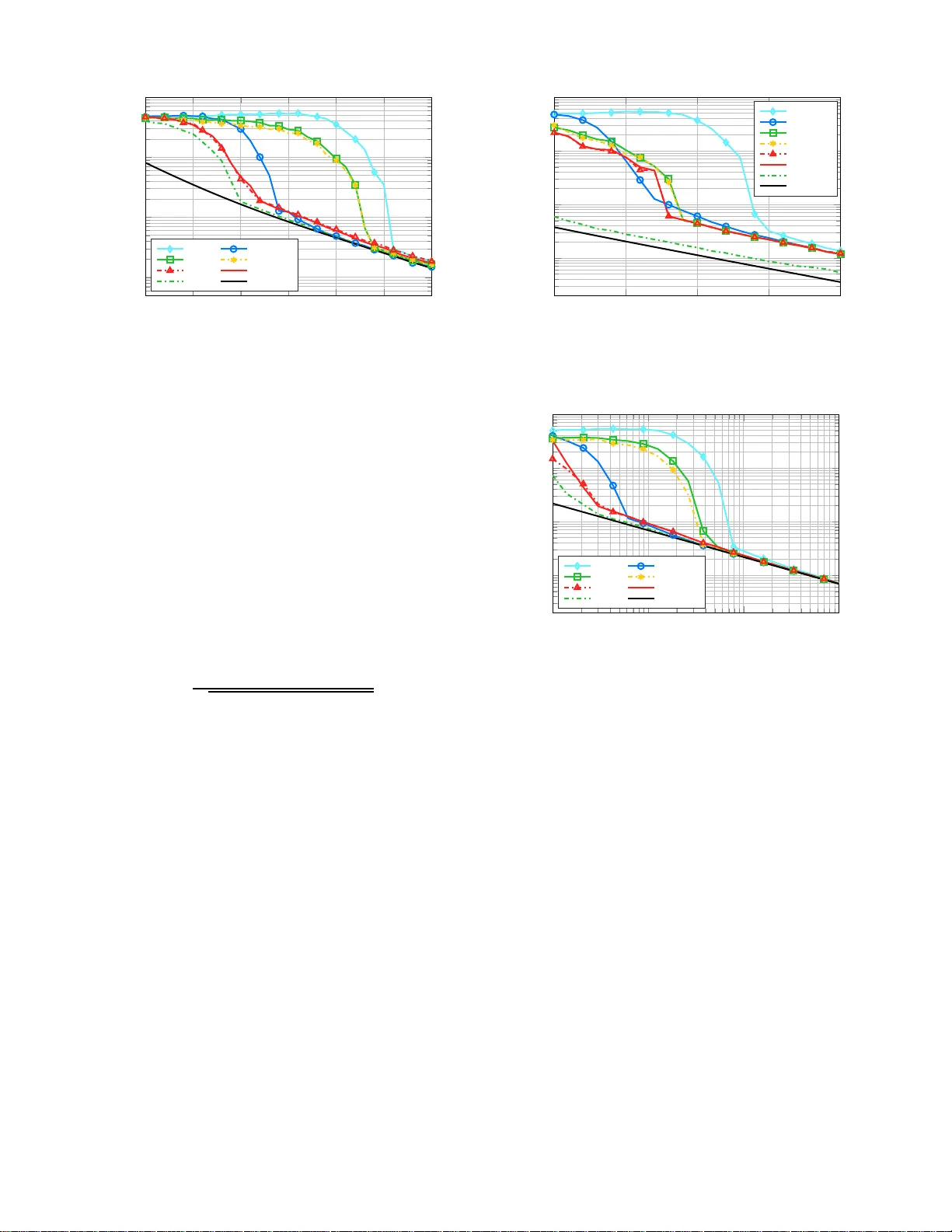
1 P artial Relaxati on Approach: An Eigen v a lue-Based DO A Estimator Frame work Minh T rinh-Hoang, Mats V iberg and Marius P esavento Abstract —In this paper , the partial relaxation approa ch is introduced and appli ed to th e DO A estimation problem using spectral search. Unlike ex isting spectral-based methods like con ventional beamf ormer , Capon beamformer or MU S IC which can be considered as single sour ce approximation of multi-sou rce estimation criteria, the pr oposed approac h accounts fo r the existence of multip le sourc es. At each co nsidered direction, the manifo ld structure of the rem aining int erfering signals impinging on the sensor array is relaxed, which results in closed f orm estimates f or the “interference” paramete rs. Th anks to this relaxa tion, the conv en tional multi-source optimization problem reduces to a simple spectral search. F ollowing this principle, we propose estimators based on the Deterministi c Maximum Likelihood, W eigh t ed Su b space Fittin g and cov ariance fittin g methods. T o calculate the null-sp ectra efficien tly , an iterative rooting scheme based on th e rational function approximation is applied to the partial relaxation methods. Simulation results show that, irrespectiv ely of any sp ecific structure of the sensor array , the perf ormance of the proposed estimato rs is superior t o the conv entional methods, especially in the ca se of low Signal-to- Noise-Ratio and low nu mber of snapshots, while maintaining a computational cost whi ch is comparable to MUSIC. Index T erms —DO A Estimation, A pproximate Maximum Like- lihood, Rank-One Modification Problem, Eigen value Decompo- sition, Least S quares Framew ork, Partial Relaxation, Rational Function Appro ximation. I . I N T R O D U C T I O N Direction-o f-Arrival (DO A) estimation an d source local- ization h av e been fund amental and long-established research directions in sensor array processing. T h e application of DO A estimation spans multiple fields of research, including wireless commun ication, radio astronomy , automotive r adar, etc. [1]– [4]. Many m ethods for DO A estimation have been developed to increase the resolution capa b ility , comp utational efficiency and robustness of the algorith ms. Although the family of Maxi- mum Likelihood (ML) estimators enjoys remar kable properties of excellen t th reshold an d asymptotic p erform ance [5]–[7], the app lication of ML estimator s in real-time scenar io s is generally impr a ctical due to the optimization o f multi-modal function s and th e associated prohibitive computational c o st. Part of this wo rk has be en acc epted for publ icatio n in 2017 IEEE In- ternati onal W orkshop on Computational Advances in Multi-Se nsor Adaptive Pr ocessing (CAMSAP 201 7) and 2018 IE E E Interna tional Confer ence on Acoustics, Speech and Signal Proc essing (ICASSP 20 18) Minh Trinh-Hoang and Marius Pesavent o are with the Communica- tion Systems Group, TU Darmstadt, Darmstadt, Germany (e-mail: thminh, pesav ento@nt.tu-darmstad t.de). Mats V iberg is with Depa rtment of Electrical Engineering, Chalmers Unive rsity of T echnology , Gothenb urg, Sweden (e-mail: mats.viber g@chalmers.se). Manuscript recei ved Nov ember 27, 2024; re vised No vember 27, 2024. In the family o f subspace-based algorithms, MUSIC [8] r e lies on th e signal sub space calculated from th e spatial sample covariance matrix and per f orms a spectral search for the estimated DOAs . In [ 9], a mo dified version of the MUSIC algorithm based on the Rando m Matrix T h eory is p roposed to improve the th reshold perfo r mance. On the other hand, root-MUSIC [10 ], ESPRIT [11] and their unitar y variants [12], [ 13], [14] exploit u niform linear and shift-in variant array structures, resp ectiv ely , to provide search-free DO A estimates, resulting in co n siderable reduction in the co m putation a l time and enha n cement in th e estimation p erform a nce [15 ]–[18 ] . When formulated as non-linear least squares (LS) problems, conv entional spectral- b ased algor ithms ign ore the existence of multiple sources in the snapshots and therefo re can be regarded as sing le source ap proxim ation of multi-source criter ia [6 ] , [19]. As a consequ ence, if the inter ference p ower f rom oth e r sources is high , the performa nce o f conv entional algorithms strongly d egrades [5 ], [2 0]. This scenario oc curs, e. g., wh en two or multiple sou rces are closely-sp a ced. T o overcome the af orementio ned shortcomin gs of exist- ing estimators with out requiring sp e cific structures of the sensor array , in this pap er , DOA estimator s based on the partial r elaxation appr oach [21] , [22] are presen ted . T aking a funda mentally different p erspective from the conventional spectral-based algo rithms, the p artial relaxa tio n appr oach takes signals from bo th “desired” and “interfering ” direction s into account. Howe ver, while the ma n ifold structure of the desired direction is u n altered, the man ifold structure of the interfering directions is relaxed to make the pr o blem com putationally tractable, hen ce the n ame partial relaxation . Based on this concept, closed-f orm expre ssion s f or the o ptimal solution s o f the relaxed in terference parameters ar e first determin ed, an d then su b stituted back into the m u lti-source criteria, resulting in s imple spectral search proce dures. In contrast to MUSIC, in which th e eigenv ectors spanning the noise sub space play an essential role in the calculation o f the null-spectrum , the partial relaxation approach r elies only o n the eigen values o f a ce r tain modified covariance matrix at each direction. In compariso n to the co rrespon d ing conv entiona l multi-so u rce fitting methods, the partial relaxation appro ach admits simpler solutions while obtaining super ior error p erform ance to the conv entional spectral- based algorithms. T o summarize, the original contributions of this pa p er ar e: • W e introduce a ne w P artial R e laxation F ramework f or the DO A estimation problem, which, from the simulation r e- sults, exh ib its excellent Signa l- to-Noise (SNR) thre shold perfor mance without requiring any p a rticular st ructur e of the sensor array . 2 • W e propose four n ew DO A estimators under the partial relaxation framew ork based on th e classical Deterministic Maximum Likelihood, W eighted Subspace Fitting, con- strained and u nconstrain ed covariance fitting estimator . • In o r der to red u ce th e overall compu ta tio nal comp lexity , we pr opose an ef ficient procedure for co mputin g th e required null-spectra o f the proposed estimato rs un der the partial relaxatio n fra mew ork. The p aper is organ ized as fo llows. The signal mode l is introdu c ed in Section II . Ex isting DO A m ethods based on non-lin e ar least squares p roblems, which are the motiv a t- ing b ackgro und of the prop o sed work, are intro duced in Section III. T he ma thematical formu la tio n of the p roposed partial relaxation ap p roach an d its adap tation to the con ven- tional DOA estimation meth ods, i.e., the Determin istic ML, W eighted Subspace Fitting, constrained and u nconstrain e d covariance fitting estimator, are described in Section IV. The computatio nal aspects of the p artial relax ation framework are discussed in Section V, where the rational approxim ation is applied to calculate the eigen values efficiently and therefore av o id the full computation of the eige n value dec o mposition . T o illustrate the perfo rmance gain in terms of estimation errors and execution time of the propo sed methods, simulation results based on sy nthetic data ar e presented in Sectio n VI. Lastly in Section VII, remarks and extension s to fu r ther r e search ar e discussed. Notatio n: Matrice s are deno ted by bold face u ppercase letters A , vectors are denoted by b o ldface lowercase letter s a , and s calars are denoted b y r egular letters a . I M represents the M × M identity matrix. Symbo ls ( · ) H , ( · ) − 1 and ( · ) 1 / 2 denote the Hermitian transp o se, inverse and the p r incipal squa r e root, respectively , o f the m atrix argument. The expectation operato r is represented by E {·} . The trace opera tor is deno ted by tr {·} , and the determ inant is represented by det ( · ) . ||·|| F denotes the Frobeniu s norm, and ||·|| 2 is th e ℓ 2 -norm of the argu m ent. Finally , N arg min f ( · ) denotes the N arguments at which the function f ( · ) attains its N -deepest separated local m inima. I I . S I G N A L M O D E L Consider an array of M sensors receiving N nar- rowband signals em itted from sources with correspo n d- ing unkn own DOAs θ = [ θ 1 , . . . , θ N ] T . Further m ore, as- sume that N < M . Th e sensor me a su rement vector x ( t ) = [ x 1 ( t ) , . . . , x M ( t )] T ∈ C M × 1 in the baseband at the time instant t is mod eled as: x ( t ) = A ( θ ) s ( t ) + n ( t ) with t = 1 , . . . , T , (1) where s ( t ) = [ s 1 ( t ) , . . . , s N ( t )] T ∈ C N × 1 denotes the baseband source signal vector from N sources and n ( t ) ∈ C M × 1 represents the ad ditive circularly comp lex noise vector at the sen sor array with the noise covari- ance matrix E  n ( t ) n ( t ) H  = σ 2 n I M . Th e steering m atrix A ( θ ) ∈ C M × N in (1 ), wh ich is assumed to have full colu mn rank, is g iv en b y: A ( θ ) = [ a ( θ 1 ) , . . . , a ( θ N )] , (2) where a ( θ n ) d enotes the sensor array response for the DO A θ n . Equatio n (1) can be rewritten for multiple snapsho ts t = 1 , . . . , T in a compact notation a s: X = A ( θ ) S + N , (3) where X = [ x (1) , . . . , x ( T )] ∈ C M × T is th e r e- ceiv ed baseb and signal m atrix. In a similar mann e r , we define the source signal matrix S ∈ C N × T and the sen- sor noise matrix N ∈ C M × T as S = [ s (1) , . . . , s ( T )] and N = [ n (1) , . . . , n ( T )] , respectively . Assume that th e sourc e signals and the noise are unco rre- lated, the covariance matrix of th e received si gnal R ∈ C M × M is given by: R = E  x ( t ) x ( t ) H  = AR s A H + σ 2 n I M , (4) where R s = E  s ( t ) s ( t ) H  is the covariance m atrix of the transmitted signal s ( t ) . W e assume through out the pa p er th at the number o f sources N is known, and the sou rce sign als are non-co herent. In practice, the tr ue cov ariance matrix R is n ot av ailable and the sample covariance matrix ˆ R is u sed instead: ˆ R = 1 T X X H . (5) Subspace techniqu es rely on the proper ties o f the eigenspaces of th e sample covariance matr ix ˆ R , which is decompo sed as: ˆ R = ˆ U ˆ Λ ˆ U H (6a) = ˆ U s ˆ Λ s ˆ U H s + ˆ U n ˆ Λ n ˆ U H n . (6b) In (6b), ˆ Λ s ∈ C N × N is a diagonal matrix, co n taining the N - largest eigenv alues { ˆ λ 1 , . . . , ˆ λ N } , an d ˆ U s ∈ C M × N contains the corresp onding N -p r incipal eigen vectors of the sample covariance matrix ˆ R . Sim ilar ly , ˆ Λ n ∈ C ( M − N ) × ( M − N ) and ˆ U n ∈ C M × ( M − N ) contain the ( M − N ) -noise eig en values { ˆ λ N +1 , . . . , ˆ λ M } and the associated noise eigen vectors, re- spectiv ely . I I I . E X I S T I N G M E T H O D S B A S E D O N N O N - L I N E A R L S In the family of ML estimators, the Deterministic ML (DML) estimates the DOAs by searching f or the steering matrix A in the N -sou rce array man ifold A N , which is parameteriz e d as follows: A N = { A | A = [ a ( ϑ 1 ) , . . . , a ( ϑ N )] , ϑ 1 < . . . < ϑ N } . (7 ) Based on the signal mo del in (3 ) and the parameterizatio n in (7), the DML estimator is formulated as the following non - linear least squa r es problem [2]: n ˆ A DML , ˆ S o = arg min A ∈A N , S ∈ C N × T || X − AS || 2 F . (8) In th e case that only the DOAs are co nsidered, the DML estimator in ( 8) c a n be re f ormulated as: n ˆ A DML o = ar g min A ∈A N tr n P ⊥ A ˆ R o . (9) In (9), P A = A  A H A  − 1 A H denotes the projection matrix onto the subspace spanned by the columns of the matrix A . 3 Similarly , P ⊥ A = I M − P A is the p rojection matrix o n to the subspace which is the orthogona l c omplemen t to the sub sp ace span ( A ) . In gene r al, the DOA estimation prob lem can be fo r mulated as: n ˆ A o = arg min A ∈A N f ( A , Y ) , (10) where f ( · ) denotes a gen eral cost f unction, and Y is a data matrix which is somehow obtained fr om the receiv ed baseband signal matrix X . W e remark that dif f erent choices on the cost function f ( · ) , the param eterization of A and the data matr ix Y result in different er r or p erform ance of the DOA estimators. Since the N -sou r ce array manifold A N is highly structur ed and non-conve x, the o ptimization problem in ( 10) is gen erally challengin g [23]–[ 2 5]. T o r e liev e the high co mputation al cost, a co mmon ap proach is to find a sub -optimal solu tio n of (10) by c onsidering a special case: the single source approximation [19], [26]. In this approach, we consider only th e single so urce array manifo ld as the feasible set of the optimization problem in (1 0 ), i.e., A = a ∈ A 1 , while lea ving the data matr ix Y unchan ged. The lo cations of N -dee pest minima of th e null- spectrum f ( a , Y ) , which are obtained by perfo rming a sweep search o n a ∈ A 1 , correspond to the steering vector s of the estimated DOAs. The above mentioned steps are compactly expressed b y the fo llowing notation : { ˆ a } = N arg min a ∈A 1 f ( a , Y ) . (11) From n ow o n , un less we want to emphasize th e dep e ndence of the steering vector a ( ϑ ) on the directio n, th e argument ϑ will be omitted. Und er the single source ap prox im ation approa c h , con ventional spectral-search DOA estimators from the literature are retrieved b y consider ing d ifferent o ptimizing criteria and different data matrices [19]: • Measurement F itting : Using the cost fun ction of the DML in (9 ) and the data matrix Y = ˆ R un der th e single sou rce appro ximation , the fo llowing op timization problem is ob tained: { ˆ a } = N arg min a ∈A 1 tr n P ⊥ a ˆ R o . (12) Note that the objective func tio n in (12) is the null- spectrum of th e conv entiona l beam former [2]. • W eighte d Subspace Fitting (WSF) : In accord ance with the DML method , the optim ization pr o blem for th e W eighted Signal Subspace Fitting is formulated in [2 3] as: n ˆ A o = arg min A ∈A N tr n P ⊥ A ˆ U s W ˆ U H s o , (13) where W ∈ C N × N is a positive semid efinite weighting matrix. In [23], th e authors showed th at by choosing the weighting matrix as: W = ˆ ˜ Λ 2 ˆ Λ − 1 s (14) with ˆ ˜ Λ = ˆ Λ s − ˆ σ 2 n I N and ˆ σ 2 n = 1 M − N M P k = N +1 ˆ λ k , the estimation erro r o f the WSF me th od as ympto tically achieves the Crame r-Rao Bo u nd as the nu m ber of snap - shots T tends to infinity . When the single source approx- imation is adop ted with the data m atrix Y = ˆ U s W ˆ U H s , we obtain the following optimization pro b lem: { ˆ a } = N arg min a ∈A 1 tr n P ⊥ a ˆ U s W ˆ U H s o . (15) In a special case when W = I N , the f ormulatio n in (15) can b e sho wn to be equiv alent to the MUSIC estimator [19]. • Covariance Fitting : Starting f rom the identity in (4) and apply ing the least squares covariance fitting with out considerin g the weig hting matrix W , we obtain [ 27]: n ˆ A , ˆ R s o = ar g min A ∈A N , R s  0       ˆ R − AR s A H       2 F . (16) If th e s ingle source consideration is adopted on (16) with the data m atrix Y = ˆ R , we obtain: { ˆ a } = N arg min a ∈A 1 min σ 2 s ≥ 0       ˆ R − σ 2 s aa H       2 F . (17) The inner optimizatio n problem in (17) obtains a closed- form minimizer ˆ σ 2 s giv en by [26 ] : ˆ σ 2 s = arg min σ 2 s ≥ 0       ˆ R − σ 2 s aa H       2 F = a H ˆ Ra ( a H a ) 2 , (18) which is merely a scaled spectru m of th e conventional beamfor mer . If a positiv e semidefinite constraint is en- forced in the inner optimizatio n prob lem in (18) as: ˆ σ 2 s = arg min σ 2 s ≥ 0       ˆ R − σ 2 s aa H       2 F subject to ˆ R − σ 2 s aa H  0 , (19) then the minimizer ˆ σ 2 s is gi ven by the Capon spectrum [26, p. 293 ], [ 2 8]: ˆ σ 2 s = 1 a H ˆ R − 1 a . (20) W e remark that the optimizatio n problems obtained by applying the single source app roximatio n appr oach to th e least squares fitting problems in ( 9), (13) and (16) are equi valent to the multi-source cr iter ia counter parts u nder the assump tions of o rthogo nal steering vectors, i.e., A H A = M I N , and unco r- related source signals. In this case, the ef f ects o f interfering signals on the desired direction vanish. As a r esult, the steer- ing vectors are de c o upled, an d the multi-source optim ization problem s c an b e deco mposed into m ultiple single source estimation pro blems. Conversely , if the steering vectors are not o rthogo nal, the performanc e of the sing le source appr oach degrades due to the interference of neighbo ring sou rce signals. I V . P A RT I A L R E L A X AT I O N A P P RO A C H In order to relieve the afo rementio n ed drawbacks of the conv entional sp ectral-search algor ithms, in this sectio n, the general concept for the partial relaxation approach is in tro- duced. Afterwards, four D OA estimator s are propo sed b y adopting the pa r tial relaxatio n ap proach on th e classical least squares pro b lems in (9), (13), (16 ) and (19). 4 A. General Concept Unlike th e sing le source approxim ation, our proposed p a r- tial re lax ation app r oach considers the signals fro m both the “desired” and “interfering” d irections. Howe ver , to make the problem tractab le, the array structu r es of the interfering sign als are relaxed. Mor e precisely , instead of enforcing the steerin g matrix A = [ a ( θ 1 ) , . . . , a ( θ N )] to be an elem ent in the highly structured ar ray man if old A N as in (10 ), without th e loss of g enerality , we maintain the manifold structure o f the first column a ( θ 1 ) of A , which cor r esponds to the signal of consideratio n. On the o ther hand, the m a nifold structure of the rem aining sources [ a ( θ 2 ) , . . . , a ( θ N )] , which ar e con sid- ered as interfering sources, is relaxed to an arbitr ary matrix B ∈ C M × ( N − 1) . Mathematically , we assume tha t A ∈ ¯ A N , where the relaxed ar ray m anifold ¯ A N is par ameterized a s: ¯ A N = n A | A = [ a ( ϑ ) , B ] , a ( ϑ ) ∈ A 1 , B ∈ C M × ( N − 1) o . (21) Note that ¯ A N still retains s ome stru cture depend ing on the ge- ometry o f the sensor ar ray , h e n ce the name partial relaxatio n. Howe ver, only one DO A can be estimated if the cost fu nction of (10 ) is min imized on the relaxed array manifold ¯ A N of (21 ). Therefo re, the grid search is app lied similarly to the single source approximation in Section III as follows: first we fix the data ma tr ix Y , minimize the ob jectiv e functio n in (10) wit h respect to B , a n d then perfo rm a grid search o n a ( ϑ ) ∈ A 1 to determin e th e locations of N -deepe st local min ima. The rationale for the partial relaxation approac h is that, each time a cand id ate DOA ϑ co in cides with one of the true DOAs θ n , then with B m odeling all other steering vectors, a perf ect fit to the data is a ttain ed at hig h SNR or large T . When ϑ is different from all true DOAs, the num ber of degrees-of- freedom in B is n ot sufficiently large to match to the data perfectly . I n the fo llowing, the par tial relaxation appro ach is applied to the fou r algorithms introduce d in Section III, i.e., th e DML, WSF , con strained and unconstrained covariance fitting estimator . B. P artially-R elaxed DML (PR-DML) Adopting th e par tial relax a tio n appro ach on the objec ti ve function in (9) leads to the f ollowing optim ization problem: { ˆ a PR-DML } = N arg min a ∈A 1 min B tr n P ⊥ [ a , B ] ˆ R o . (22) By rewriting the objective f unction in (22) to deco uple a an d B p artially , we ob tain: tr n P ⊥ [ a , B ] ˆ R o = tr n P ⊥ a ˆ R o − tr n P P ⊥ a B ˆ R o , (23) where we use the conv ention that tr n P P ⊥ a B ˆ R o = 0 if P ⊥ a B = 0 . Since the first term on the right h a nd side of (23) does not depen d o n B , the inner op timization pr oblem in (22 ) is equiv a len t to: max B tr n P P ⊥ a B ˆ R o . (24) The solution o f (24) is gi ven b y (see Appen dix A): max B tr n P P ⊥ a B ˆ R o = N − 1 X k =1 λ k  P ⊥ a ˆ R  , (25) where λ k ( · ) denotes the k -th largest eigenv alue of the matr ix in the a rgu ment. Substituting (2 3) an d (2 5 ) ba c k into the objective func tion o f (2 2 ), the null-spectru m o f the PR-DML estimator is ob ta in ed as: f PR-DML ( ϑ ) = min B tr n P ⊥ [ a ( ϑ ) , B ] ˆ R o = M X k = N λ k ( P ⊥ a ( ϑ ) ˆ R ) . (26) The estimated DO As ˆ θ = h ˆ θ 1 , . . . , ˆ θ N i T are th e n determin ed by cho osing the lo cations of the N -d eepest minima of the n ull- spectrum f PR-DML ( ϑ ) . As fur ther e la b orated in Section V, the null-spectru m f PR-DML ( ϑ ) in ( 2 6) can be efficiently comp u ted without necessarily perf orming a full eigen value deco m posi- tion at each direction, i.e., computin g the correspond ing set of eigenv ectors of th e matrix P ⊥ a ( ϑ ) ˆ R is n ot require d . C. P artially-Rela xed WS F (PR-WSF ) Follo wing a similar der ivation as fo r the PR-DML estimato r in Section IV -B and using th e math ematical formulatio n o f the WSF estimator in (15), the o p timization p r oblem corre spond- ing to th e PR-WSF estimator re a d s: { ˆ a PR-WSF } = N arg min a ∈A 1 min B tr n P ⊥ [ a , B ] ˆ U s W ˆ U H s o , (27) and the nu ll-spectrum of the PR-WSF is calculated as: f PR-WSF ( ϑ ) = M X k = N λ k ( P ⊥ a ( ϑ ) ˆ U s W ˆ U H s ) . (28) Note th a t in a special case when W = I N , the pro p osed estimator in (27) is eq uiv alent to the MUSIC estimator (see Append ix B). Fr om now on, if not f urther specified, the weighting matrix W is cho sen as in ( 14). D. P artially-Re laxed Constrained Covariance F itting ( PR- CCF) T o deriv e new estimators based on th e covariance fitting problem s in (18 ) and (1 9), we follow the p rinciple of the partial relaxa tion approac h for th e arr ay steering matrix by relaxing A = [ a , B ] with an arbitrary matrix B ∈ C M × ( N − 1) . Similarly , we p a rtition the w aveform matrix S = h s , J T i T in the signa l mod el in (3) with s ∈ C T × 1 and J ∈ C ( N − 1) × T to obtain: X = as T + E + N , (29) where E = B J ∈ C M × T models the recei ved sign al of th e remaining ( N − 1) -sources with the relaxed array manifold structure an d therefo re rank ( E ) ≤ N − 1 . Furtherm ore, we as- sume that the sample covariance matrix ˆ R is positi ve defin ite, and the si gnals from other so u rces are uncorrelated with t he signals from the direction a . Similar to the Capon beamform er in (19), the partially- r elaxed con strained c ovariance fitting (PR-CCF) prob lem is f ormulated as f ollows: { ˆ a PR-CCF } = N arg min a ∈A 1 min σ 2 s ≥ 0 , E       ˆ R − σ 2 s aa H − E E H       2 F subject to ˆ R − σ 2 s aa H − E E H  0 subject to rank ( E ) ≤ N − 1 . (30) 5 Keeping  σ 2 s , a  fixed and minimizing the objective function of ( 30) with respect to E , a low-rank appr o ximation problem is obtained as [29]: min E       ˆ R − σ 2 s aa H − E E H       2 F = M X k = N λ 2 k ( ˆ R − σ 2 s aa H ) . subject to r a n k ( E ) ≤ N − 1 (31) By perf orming the eigenv alue decom p osition: ˆ R − σ 2 s aa H = ˜ U s ˜ Λ s ˜ U H s + ˜ U n ˜ Λ n ˜ U H n , (32) where ˜ Λ s and ˜ U s contain the ( N − 1) - largest eigen values and the correspo nding principal e ig env ectors of ˆ R − σ 2 s aa H , respectively , a minimizer ˆ E o f (31) satisfies: ˆ E ˆ E H = ˜ U s ˜ Λ s ˜ U H s . (33) Substituting the minim iz e r ˆ E in ( 3 3) back to the inne r op- timization problem in (30), we o bserve tha t, the co n straint ˆ R − σ 2 s aa H − ˆ E ˆ E H  0 implies that ˆ R − σ 2 s aa H  0 . Con versely , for each σ 2 s ≥ 0 , if ˆ R − σ 2 s aa H  0 , from (32) and (33), we co nclude th at ˆ R − σ 2 s aa H − ˆ E ˆ E H  0 . As a consequen ce, an equiv alent f ormulatio n of th e inner problem in (30 ) is obtained as fo llows: min σ 2 s ≥ 0 M X k = N λ 2 k ( ˆ R − σ 2 s aa H ) subject to ˆ R − σ 2 s aa H  0 . (34) It can be easily shown fro m the W eyl’ s inequality re gard in g the eigen values of the modified Hermitian matrix [ 30] and the positive semid efiniteness of ˆ R − σ 2 s aa H that, as long as the constrain t in (34) is n ot violated, the ob je c tive function in (34) is strictly decreasing as σ 2 s increases. Therefo r e, ˆ σ 2 s, C is a minimizer of (3 4 ) if an d on ly if the matrix ˆ R − ˆ σ 2 s, C aa H possesses at least one eigenv alu e equ al to zero. Consequently , the minimizer ˆ σ 2 s, C is obtained f rom the Cap on sp ectrum [26, Equation (6.5 .33)] : ˆ σ 2 s, C = 1 a H ˆ R − 1 a . (35) Substitute (34) an d (3 5) back into (30), the PR-CCF estimator returns the estimate d DOAs by determinin g the N -deepe st minima of the following null-spectr um: f PR-CCF ( ϑ ) = M X k = N λ 2 k ˆ R − 1 a ( ϑ ) H ˆ R − 1 a ( ϑ ) a ( ϑ ) a ( ϑ ) H ! . (36) If th e sample covariance m atrix ˆ R is singu lar , the nu ll- spectrum of the PR-CCF estima to r cannot be computed using (36). Howe ver, the diagon al loading technique [ 28], [31] c a n be applied o n the sample covariance matrix ˆ R . The choice on the lo ading factor γ and its influen ce on the estimation perfor mance are sub ject of futur e research. E. P artially-R elaxed Unconstrained Covariance F itting (PR- UCF) Comparing with the constrain ed version pr e sented in Sec- tion IV -D, the formu lation of the PR-UCF om its the p ositiv e semidefiniteness constraint to yield the f ollowing optimization problem : { ˆ a PR-UCF } = N arg min a ∈A 1 min σ 2 s ≥ 0 , E       ˆ R − σ 2 s aa H − E E H       2 F subject to r a n k ( E ) ≤ N − 1 . (37) When min imizing with resp ect to E , the minim iz e r ˆ E o f the o p timization pro b lem in (37) is obtain ed from the best rank- ( N − 1) app roxima tion of ˆ R − σ 2 s aa H as describe d in (32) and (3 3). Hence, the inner optimization of th e PR-UCF estimator at each direction a = a ( ϑ ) is: min σ 2 s ≥ 0 M X k = N λ 2 k  ˆ R − σ 2 s aa H  . (38) Unlike th e constrain ed variant in (34 ), the minimizer of g ( σ 2 s ) = M P k = N λ 2 k  ˆ R − σ 2 s aa H  in (38) with respect to σ 2 s , d enoted as ˆ σ 2 s, U , d oes no t have a closed form solu tion. Howe ver, a numerical solution of ˆ σ 2 s, U can be deter m ined by noting th a t the function g ( σ 2 s ) is continuo usly differentiable, and the der i vati ve g ′  σ 2 s  is given by (see Ap pendix C): g ′  σ 2 s  = − M X k = N 2 ¯ λ k ( σ 2 s ) σ 4 s a H  ˆ R − ¯ λ k ( σ 2 s ) I M  − 2 a , (39) where we in troduce the following shorthan d notation : ¯ λ k ( σ 2 s ) = λ k  ˆ R − σ 2 s aa H  . (40) Note that the denomin ator in each sum m and of the expression in (39) is a lways po sitive, we ob serve that: • If σ 2 s → 0 , then ¯ λ k ( σ 2 s ) ≥ 0 with k = N , . . . , M and therefor e: lim σ 2 s → 0 g ′  σ 2 s  < 0 . (41) • If σ 2 s → ∞ , the rank- one componen t − σ 2 s aa H is dominan t to ˆ R and thu s we obtain an asy m ptotic r esult for the smallest eig en values ¯ λ M  σ 2 s  as follows: lim σ 2 s →∞ ¯ λ M  σ 2 s  σ 2 s || a || 2 2 = − 1 . (42) In a d dition, th e rem aining eig en values ¯ λ k  σ 2 s  with k = N , . . . , ( M − 1) are a lways bo u nded above an d be- low thanks to the W eyl’ s inequality [3 0]. Applying this remark and the id entity in ( 42) to (3 9 ) lead s to: lim σ 2 s →∞ g ′  σ 2 s  = ∞ . (43) From ( 39), (41) and ( 4 3), there exists a sufficiently small σ 2 s, left and a sufficiently large σ 2 s, right so that the sign of the deriv ativ e g ′  σ 2 s  changes fr om negative to positive in the interval h σ 2 s, left , σ 2 s, right i . T herefor e, a simple bisection search [32] can a p plied to com pute the minim izer ˆ σ 2 s, U of (3 8). The steps to d etermine a sear ch interval fo r the bisectio n search an d the computation of the null-spectrum of the PR-UCF estimator at each dir ection a ( ϑ ) are summarized in Algorithm 1. 6 Algorithm 1 Calculating the null-spectrum of PR-UCF at a giv en direction a = a ( ϑ ) 1: Initialization : σ 2 s, left = σ 2 s, right > 0 , to lerance ǫ , the deriv ativ e g ′  σ 2 s,  defined in (3 9) 2: if g ′  σ 2 s, left  < 0 t hen 3: repeat 4: σ 2 s, right ← 2 σ 2 s, right 5: until g ′  σ 2 s, right  > 0 6: else 7: repeat 8: σ 2 s, left ← σ 2 s, left / 2 9: until g ′  σ 2 s, left  < 0 10: end if 11: Determine the root ˆ σ 2 s, U of (3 9) by bisectio n search o n h σ 2 s, left , σ 2 s, right i with the toler ance ǫ 12: return f PR-UCF ( ϑ ) = M P k = N λ 2 k  ˆ R − ˆ σ 2 s, U a ( ϑ ) a ( ϑ ) H  V . C O M P U TA T I O N A L A S P E C T S O F T H E P A RT I A L R E L A X AT I O N M E T H O D S As in troduced in Section IV, the prop osed partial r elaxation approa c h in volves the e stimation proc e dures which r equire extensi ve eigenv a lu e compu tation for th e ev alu ation of the null-spectru m over th e e ntire angle-of- view . In fact, the null- spectra in ( 26), (28) an d (36) and Algor ithm 1 depe nd o nly on th e eige nvalues, and therefor e the explicit co m putation of the eigen vectors can be avoided. Gen erally , if no par- ticular stru c tu re of the matr ix is exploited, the eigenv alue decomp o sition requires O ( K 2 L ) ope r ations where K is the dimension o f the m atrix an d L is the n umber of requir ed eigenv alu es [ 3 3, Ch. 8]. This com putationa l co mplexity may be pr ohibitive for specific p ractical ap plications and lim it the usage of the pr oposed partial relaxation app roach in practice if no a cceleration pro cedure is considered. Furtherm ore, from an algorithm ic per spectiv e, the expr essions in Equation (2 6), (28), (36) and Algor ithm 1 share a commo n und e rlying pr oblem structure in th e sense th a t th ey all requ ire, as a main task, the computatio n of the eigen values o f a generic matrix fo rm as follows: D − ρ z z H = ¯ U ¯ D ¯ U H . (44) In (44), D = diag ( d 1 , . . . , d K ) ∈ R K × K is a constant real diagona l matrix , ρ ∈ R is an arb itrary positive real scalar an d z = [ z 1 , . . . , z K ] T ∈ C K × 1 is a d irection-d epende n t co mplex- valued vector . The relationship between the generic f orm in (44) and the null-spectra in (26), (28 ), (3 6) an d Algorith m 1 is furthe r detailed in the sectio ns below . Since the expression on th e left hand side o f (4 4 ) denote s a Her mitian matrix obtained by subtrac tin g a r a nk-on e matrix fr om a constant diagona l matrix, the term r ank-o ne mod ifi ed Hermitian matrix is ad opted. As presen ted in the following sections, this par ticu- lar structu re allows a faster im p lementation of the e igenv alu e decomp o sition, an d thus acce ler ates the comp utation of th e null-spectru m of the partial relaxation estimator s. A. Eigen value Decomposition of a Rank - One Modified Her - mitian Matrix Initially p roposed by Bunch, Nielsen and Sorensen in [34 ] as a suppo rt for calculating the eigenv alues and eigen vectors of symmetric tridiagonal ma tr ices in par allel, th e procedu r e of determining a c omplex-valued eigensystem of a ra nk-on e modified Hermitian matrix is based on the in terlacing th eorem as follows [3 3, p. 47 0]: Theor em 1: Le t { d 1 , . . . , d K } be the elemen ts on the diagona l of the matrix D ∈ R K × K where { d 1 , . . . , d K } are distinct and sorted in descending order . Further assume that ρ > 0 an d z ∈ C K × 1 contains only non- z ero entries. If the eigenv alu es  ¯ d 1 , . . . , ¯ d K  of the matrix D − ρ z z H are also sorted in descen d ing order, then: •  ¯ d 1 , . . . , ¯ d K  are th e K zeros of the secular f unction p ( x ) = 0 , where p ( x ) is given by: p ( x ) = 1 − ρ z H ( D − x I K ) − 1 z (45) = 1 − ρ K X k =1 | z k | 2 d k − x . (46) •  ¯ d 1 , . . . , ¯ d K  satisfy the inter la c in g p roperty , i.e., d 1 > ¯ d 1 > d 2 > ¯ d 2 > . . . > d K > ¯ d K . ( 47) • The eig en vector ¯ u k associated with th e eig en value ¯ d k is a multiple of  D − ¯ d k I K  − 1 z The special cases of r epeated elements in the diag onal matrix D and zero-valued entries in z are tr eated in Append ix D. Based o n Th eorem 1 , roo ting the secular fun ction in (46 ) is of great impo rtance f or the acceleratio n of o u r propo sed partial relaxation app r oach. Du e to the structure of th e secular function in (46) and th e interlacing property in (4 7), the zeros of the secular function can be determined indepen dently of each o ther, th us allo wing further improvement in th e execution time throug h pa r allel computing. W itho ut loss of generality , consider the k -th roo t of the secular function ¯ d k which lies inside the interval ( d k +1 , d k ) where k = 1 , . . . , K and d K + 1 = −∞ . By defining the two au xiliary ra tional f unction s: ψ k ( x ) , − ρ k X j =1 | z j | 2 d j − x (48) φ k ( x ) ,      − ρ K P j = k +1 | z j | 2 d j − x if 1 ≤ k ≤ K − 1 0 if k = K , (49) the secular fun ction in (46 ) can be rewritten a s: − ψ k ( x ) = 1 + φ k ( x ) . (50) Since b oth ψ k ( x ) and φ k ( x ) are define d as the sum of m ultiple rational fu nctions, a straightfo rward approach to solve ( 50) iterativ ely fro m a given point x ( τ ) is using rational functions of fir st d egree ˜ ψ k ( x ) and ˜ φ k ( x ) , respectiv ely , as approxim ants. The author in [35, Subsec. 2.2.3 ] suggests the approx imant o f type: R k ; p,q ( x ) =    p + q d k +1 − x if 0 ≤ k ≤ K − 1 0 if k = K , (51) 7 Algorithm 2 Determining the k -th root o f the secular function 1: Initialization : Iteration index τ = 0 , arbitrary starting value x (0) ∈ ( d k +1 , d k ) , toleran ce ǫ 2: repeat 3: Find the p arameters p and q such tha t: R k − 1; p,q ( x ( τ ) ) = ψ k ( x ( τ ) ) (52) R ′ k − 1; p,q ( x ( τ ) ) = ψ ′ k ( x ( τ ) ) (53) 4: Find the p arameters r and s such that: R k ; r,s ( x ( τ ) ) = φ k ( x ( τ ) ) (54) R ′ k ; r,s ( x ( τ ) ) = φ ′ k ( x ( τ ) ) (55) 5: Find x ( τ +1) ∈ ( d k +1 , d k ) wh ich satisfies: − R k − 1; p,q ( x ( τ +1) ) = 1 + R k ; r,s ( x ( τ +1) ) (56) 6: τ ← τ + 1 7: until   x ( τ +1) − x ( τ )   < ǫ 8: return ¯ d k = x ( τ +1) and choosing the parameters p and q such that the ap proxi- mants coincide at a giv en p oint x ( τ ) with the correspon ding exact fu nctions in (4 8) an d (49), respectiv ely , up to the first- order d eriv ati ve. A special case is obtain ed when k = K , in which ˜ φ K ( x ) , 0 is c hosen. Different ch o ices of the approx imants were also introduced and discussed in [ 35], [ 3 6]. For con venience purposes, the steps for deter m ining the ro o ts of the secular function in (46) are summar ized in Algorithm 2. Since the approx imant in (51) is a r ational fun ction of degree one, the steps in (52 )-(56) can be solved in closed for m and th us the complexity of each iteration τ is O ( K ) . As a result, the overall comp lexity of the eig en value d ecompo sition proced u re is O ( K LI ) , wh ere L is the number o f required eigenv alu es, and I is the number of iterations required f or the conv ergence of Algorithm 2. Note that Algo rithm 2 converges quadra tica lly [35], a n d wh e n applied to the partial relaxation methods on a fine grid, the eigenv a lu es for o ne directio n c a n be used as a starting po int f or the e igenv alu es at the next d ir ection. From the simulation results, th e numb e r of iteration I requir e d for the toler ance ǫ = 1 0 − 9 is less th an 4. The r efore, we can assume that the comp lexity o f the compu tational eigen value decomp o sition using Alg orithm 2 is o f order O ( K L ) . B. Applica tio n to P R-DML As mentioned in Section V -A, the complexity of e valuating the null-spectrum is pro portion al to the number o f r equired eigenv alu es L . Therefore, to accelerate the com putation of the null-spectru m o f the PR-DM L meth od, we reduce the number of r equired eigenv alues by rewriting the expression in (2 6) as follows: M X k = N λ k  P ⊥ a ˆ R  = tr n P ⊥ a ˆ R o − N − 1 X k =1 λ k  P ⊥ a ˆ R  = tr n ˆ R o − a H ˆ Ra a H a − N − 1 X k =1 λ k  P ⊥ a ˆ R  . (57) Using the reformulation in (57), o nly ( N − 1) - eig en values out o f M eig en values o f P ⊥ a ˆ R are comp uted, and therefo r e the co mputation al com plexity is reduce d . In order to apply the eigenv alu e d ecompo sition p rocedu re p resented in Section V -A, the term λ k  P ⊥ a ˆ R  is furthe r rewritten as follows: λ k  P ⊥ a ˆ R  = λ k  ˆ R 1 / 2 P ⊥ a ˆ R 1 / 2  = λ k ˆ R − 1 || a || 2 2 ˆ R 1 / 2 aa H ˆ R 1 / 2 ! = λ k ˆ Λ − 1 || a || 2 2 ˆ Λ 1 / 2 ˆ U H aa H ˆ U ˆ Λ 1 / 2 ! . (58) From the expression in (58), the eigenv alu e decomp osition proced u re introduc e d in Sec tio n V -A is ap plied with D = ˆ Λ , ρ = 1 || a || 2 2 and z = ˆ Λ 1 / 2 ˆ U H a . Fro m the comp utational per- spectiv e, excep t for th e initial full eig e nvalue de c omposition in (6a), the overall co mplexity of the calculatio n of the null- spectrum for the c omplete ang le-of-v iew with N G directions is O  M 2 + M ( N − 1)  N G  = O ( M 2 N G ) . This is h ig her than the complexity requir ed for comp uting the MUSIC null- spectrum, which is O ( M N N G ) . C. Application to PR-WSF A similar iterativ e pr ocedur e fo r com p uting the eigenv alu e decomp o sition as pr oposed in Section V -A and Section V -B can be app lied dire ctly to the PR-WSF metho d pr esented in Section IV -C. Howe ver , the compu tational c o mplexity o f the PR-WSF metho d can b e e ven further redu ced due to the fact that all eigenv alues λ k ( P ⊥ a ˆ U s W ˆ U H s ) with k = N + 1 , . . . , M are equal to zer o since r a n k ( P ⊥ a ˆ U s W ˆ U H s ) ≤ N . Therefo re, only the N -th eigenv alue λ N ( P ⊥ a ˆ U s W ˆ U H s ) n eeds to be calculated. Fu r thermor e, the dim e nsion of the ma trix D in (44) can also be re d uced. In fact, similar to (57), it ca n be shown that: λ N  P ⊥ a ˆ U s W ˆ U H s  = λ N W − 1 || a || 2 2 W 1 / 2 ˆ U H s aa H ˆ U s W 1 / 2 ! . (59) Using the identity in (59), the pr ocedur e for co mputing the eigenv alu e decom position in troduc e d in Section V -A is applied with D = W , ρ = 1 || a || 2 2 and z = W 1 / 2 ˆ U H s a . Since the dimension of the m atrix is reduced fro m M × M to N × N , and only a single eige n value is requ ired, the com plexity reduce s to O (( N M + N − 1) N G ) = O ( M N N G ) , which is identical to the co mputation al complexity of the MUSIC algo rithm. Howe ver, th e comp utational overhead associated with PR- WSF is still higher than MUSIC since in the prepr o cessing step, additional calculation for d etermining the weighting matrix D = W and the vecto r z = W 1 / 2 ˆ U H s a is re quired. D. Applicatio n to PR -CCF The expression of th e PR-CCF null-spectrum in ( 3 6) re- sembles the ge neric formu lation of th e rank- one m odified 8 Hermitian matrix in (4 4), except for the fact th at the matrix ˆ R is g enerally not diagon al. Theref ore, the a p plication o f the eigenv alu e d ecompo sition in Section V -A is straigh tforward, in which we perf orm an or thogon al tran sformation on ˆ R and a to diagonalize ˆ R . Howe ver, the number of the eigen values r e- quired for the computation of the null-spectru m is ( M − N + 1) , which is typically larger than the n umber of sou r ces N . By rewriting the expression in (36) using the trace operator, only the ( N − 1) -largest e igenv alu es are calculated and the null- spectrum of the PR-CCF m ethod is rewritten in the f ollowing form to utilize the principa l eigenv alues: M X k = N λ 2 k  ˆ R − ˆ σ 2 s, C aa H  = M X k = N λ k   ˆ R − ˆ σ 2 s, C aa H  2  = tr   ˆ R − ˆ σ 2 s, C aa H  2  − N − 1 X k =1 λ 2 k  ˆ R − ˆ σ 2 s, C aa H  = tr n ˆ R 2 o − 2 ˆ σ 2 s, C a H ˆ Ra + ˆ σ 4 s, C || a || 4 2 − N − 1 X k =1 λ 2 k  ˆ R − ˆ σ 2 s, C aa H  . (60) Considering the for mulation in (60), we obser ve that th e PR- CCF method in volves both the con ventional and Capon beam - former in the e valutaion of the null-sp e ctrum. Similarly to th e PR-DML method, for any eigenv a lu e λ k  ˆ R − ˆ σ 2 s, C aa H  , it can be sh own that: λ k  ˆ R − ˆ σ 2 s, C aa H  = λ k  ˆ Λ − ˆ σ 2 s, C ˆ U H aa H ˆ U  . (61) From (60) and (61), we apply the eige nvalue decomp o sition proced ure presented in Sectio n V -A with D = ˆ Λ , ρ = ˆ σ 2 s, C and z = ˆ U H a . Thus, the overall computatio nal co mplexity of the PR-CCF algorith m is O  M 2 + M ( N − 1)  N G  = O ( M 2 N G ) . E. Applica tio n to P R-UCF Unlike the PR-DML, PR-WSF and PR-CCF estimato rs, the PR-UCF estimator r e quires add itional steps o f calcu lating the der iv ative g ′ ( σ 2 s ) in ( 39) to o btain the minimizer σ 2 s, U of (38). T o re duce the numb er o f required eigenv alu e s for computin g the derivati ve and th e nu ll-spectrum, the functio n g ( σ 2 s ) = M P k = N λ 2 k  ˆ R − σ 2 s aa H  is rewritten similarly to (6 0) as follows: g ( σ 2 s ) = tr n ˆ R 2 o − 2 ˆ σ 2 s a H ˆ Ra + ˆ σ 4 s || a || 4 2 − N − 1 X k =1 λ 2 k  ˆ R − ˆ σ 2 s aa H  . (62) The derivati ve g ′  σ 2 s  is calcu lated as: g ′  σ 2 s  = − 2 a H ˆ Ra + 2 σ 2 s || a || 4 2 + N − 1 X k =1 2 ¯ λ k ( σ 2 s ) σ 4 s a H  ˆ R − ¯ λ k ( σ 2 s ) I M  − 2 a (63) where ¯ λ k ( σ 2 s ) = λ k  ˆ R − σ 2 s aa H  . By sub stituting z = ˆ U H a , we ob tain: ¯ λ k ( σ 2 s ) = λ k  ˆ Λ − σ 2 s z z H  (64) g ′  σ 2 s  = − 2 z H ˆ Λ z + 2 σ 2 s || z || 4 2 + N − 1 X k =1 2 ¯ λ k  σ 2 s  σ 4 s M P j =1 | z j | 2  ˆ λ j − ¯ λ k ( σ 2 s )  2 . (65) Based o n the expr essions in (64) an d (6 5), th e null-spectrum of PR-UCF fr om Alg orithm 1 is calculated by apply ing the proced u re in Sectio n V -A with D = ˆ Λ , ρ = σ 2 s , 0 and z = ˆ U H a . T h e compu tational complexity of the PR-UCF meth o d is therefo re of or der O ( M 2 N G N I ) wh ere N I is the n umber of bisection steps conducted in Algo r ithm 1 . V I . S I M U L AT I O N R E S U LT S In this section, s imulation results r egar ding the performance of different DOA estimators are p resented and compared with the stocha stic Cramer-Rao Bou n d (CRB) [ 7]. The nu mber of Mon te - Carlo runs is N R = 10 00 . The key perform ance indicators are th e Roo t-Mean-Sq uared-E rror (RMSE), which is calculated as: RMSE = v u u t 1 N R N N R X r =1 N X n =1  ˆ θ ( r ) n − θ n  2 , (66) and the execution time of each Mon te-Carlo run. The estimated DO As in th e r -th Monte-Carlo r un ˆ θ ( r ) = [ ˆ θ ( r ) 1 , . . . , ˆ θ ( r ) N ] T and th e true DOAs θ = [ θ 1 , . . . , θ N ] T in (66) are sorted in ascending o rder . Th e simulation s a r e con ducted in MA TLAB 2016b on a PC equ ipped with an O S of Arch L inux with a processor 8 x Intel Core i7-67 00 4.00 GHz CPU and 16GB RAM. T h e iterative eigenv alue decom position intr o duced in Section V -A is implem ented in C an d imported in MA TLAB throug h a MEX interface. I n o u r simulatio ns, if not further specified, we assume two uncorrelated but closely space d source signals at θ = [45 ◦ , 5 0 ◦ ] T which impin g e on a ULA of M = 10 antennas w ith the spacing equal to half of the wa velength. W e stress th a t unlike roo t-MUSIC, a ll PR me thods are applicable to any array geom etry . The source signals ha ve the mean value of zero and unit po wer . The SNR is calcu lated as SNR = 1 σ 2 n . Regard ing the PR-WSF method , we choose the weighting as in (1 4 ). Since we consider only two source signals, the DO A estimations from th e DML estimator can be o btained by perfo rming a bru te-force search f or the global maximum of th e o bjective functio n in (9 ) over a d e nse grid on A 2 . As dep icted in Figure 1, the partial relaxation m ethods exhibit superior SNR threshold perfor mance in comparison to the MUSIC algorithm . The PR-CCF and PR-UCF estimato r possess alm ost identical estimatio n err or perfo rmance in th e inspected SNR r egion, wh ere their thresholds occur at an ev en lower SNR than that of r oot-MUSIC. Th e PR-CCF and PR-UCF a re ou tperfor m ed b y the brute- f orce D M L in both the asym ptotic an d the n on-asym ptotic regions, althoug h the 9 − 10 − 5 0 5 10 15 20 10 − 1 10 0 10 1 10 2 SNR (dB) RMSE (deg) MUSIC root -MUSIC PR-DML PR-WSF PR-CCF PR-UCF DML CRB Figure 1 : Uncorr elated source signals, number o f sn apshots T = 40 difference in RMSE is sm a ll. This remark su g gests that PR- CCF is more fa vorable than PR-UCF , since the computation al complexity of PR-CCF is lower than that of PR-UCF while the error perfo rmances are comp arable. Th e RMSE o f both PR- CCF and PR-UCF does not app roach th e CRB. However , the difference in RMSE is insignificant. PR-DML a n d PR-WSF have similar per forman ce beh aviors, achieving the CRB at a lower SNR than MUSIC but m uch high er th an root- M USIC. In the next simulation, we consider the cor related signals o f two sources. The co rrelation coefficient ρ is defined as: ρ = E  s 1 ( t ) H s 2 ( t )  r E n | s 1 ( t ) | 2 o E n | s 2 ( t ) | 2 o . (67) In Figure 2, th e correlation coe fficient is set to ρ = 0 . 95 . The number of snapshots is incr eased to T = 20 0 . No te that spa tial smoothing [37], [ 38] or forward- backward averaging [ 39] is not applied . DML consistently outpe r forms oth er consider e d estimators in the inspected SNR region. The threshold of root- MUSIC now occur s at a slightly lo wer SNR than that of the partial r elaxation m ethods. On the o ther hand, in the post- threshold region, all estimators un der the partial relax ation framework have a lower RMSE th an roo t- MUSIC. Ho wever , the imp r ovement in RMSE is n egligib le. In the next simulation, as depicted in Figure 3, the SNR is fixed at 3 dB, and the n umber of snapsho ts T is v aried between 10 and 1 0000. The RMSE pe r forman ce o f PR- UCF/PR-CCF resemb les that of DML, achieving the asymp - totic region at T = 30 sample s, which is appro ximately an order of magnitud e lower in the required snap shots than that for PR-DML/PR-WSF . However , in the post-thresho ld region, the RMSE of PR-CCF and PR-UCF is n ot as close to the CRB as th at of r o ot-MUSIC, PR-DML or PR-WSF . PR- WSF outperfo r ms PR-DML consistently in this simulation . In general, the p artial relaxation meth o ds o u tperfor m MUSIC. In the four th setup , the DO A of the first source signal is fixed at θ 1 = 45 ◦ and the an g ular separation between two sources 5 10 15 20 25 10 − 1 10 0 10 1 10 2 SNR (dB) RMSE (deg) MUSIC root-MUSIC PR-DML PR-WSF PR-CCF PR-UCF DML CRB Figure 2: Correlated source signals with ρ = 0 . 95 , num ber of snapshots T = 200 10 1 10 2 10 3 10 4 10 − 1 10 0 10 1 10 2 Number of Snapshots RMSE (deg) MUSIC root -MUSIC PR-DML PR-WSF PR-CCF PR-UCF DML CRB Figure 3: Uncorrelated so urce signals, SNR = 3 dB ∆ θ is varied from 0 . 5 ◦ to 6 ◦ . In Figure 4, similar to DML , the RMSE of PR-CCF/PR-UCF is close to the Cram er-Rao Bound even when the angular separation ∆ θ is as small as 1 . 25 ◦ , which is significan tly smaller than th e angular sep ara- tion req uired for PR-DML/PR-WSF to r esolve two so urces. Howe ver, the RMSE o f PR-CC F/PR-UCF slowly achie ves the CRB o nly when ∆ θ > 5 ◦ . PR-WSF slightly outperfo rms PR- DML, and bo th algorith m s outp erform MUSIC. Figure 5 dep icts a scenario where th e number of snapsh o ts T = 8 is smaller th an the nu mber of an te n nas M = 1 0 . In th is case, the sample covariance matrix calcu lated in (5) is singu lar , and therefor e the PR-CCF is not ap p licable. I n this case, we apply the d iagonal loadin g techniqu e with the lo a ding factor γ = 10 − 4 on th e sample covariance matrix. The initialization of σ 2 s, left in Algo rithm 1 is set at 10 − 6 . T o av oid outliers in RMSE caused by misdetection and to simu late the DOA tracking process [40], 1% of th e estimates with the largest erro r for all inv estigated alg o rithms are removed before calculating the RMSE. I t ca n be obser ved that, even in the case of a very low number of snapshots, PR-UCF obtain s a rema rkable threshold beh avior , outperf orming other methods except f or the brute- force DML. The RMSE o f PR-UCF only slowly approa c h es th e Cramer-Rao Bound as th e SNR increases. In 10 1 2 3 4 5 6 10 − 1 10 0 10 1 10 2 Angular Separation ∆ θ (deg) RMSE (deg ) MUSIC root -MUSIC PR-DML PR-WSF PR-CCF PR-UCF DML CRB Figure 4: Uncorrelated source signals, SNR = 10 dB, n umber of snapsho ts T = 100 0 5 10 15 20 25 30 10 − 1 10 0 10 1 10 2 SNR (dB) RMSE (deg) MUSIC root -MUSIC PR-DML PR-WSF PR-CCF PR-UCF DML CRB Figure 5 : Uncorr elated source signals, number o f sn apshots T = 8 the high SNR regime, however , the RMSE of PR-UCF is very close to the Cramer-Rao Bound . The pe r forman ce o f PR- CCF is highly d egraded du e to the diagonal loading. Further research may b e ca r ried out regard ing the op timal adaptive choice of the diago nal loadin g factor γ to achieve an improved perfor mance using a d irection-d ependen t factor . Ho wever , this is b eyond the sco p e of this paper, an d therefo re left for further research. Similar to the above-in vestigated scenario s, PR-DML and PR-WSF o utperfo rm MUSIC consistently . In Figu re 6, the execution time of th e DOA estimation algorithm s with respect to the numbe r of anten nas M are d e- picted. W e do not include the brute-forc e DML d ue to the high execution time. The angle-o f-view is p artitioned unifor mly into N G = 1800 directions. The term Generic in Figu re 6 r efers to the naive im plementation usin g the MA TLAB comman d eig for the eigenvalue decom p osition. The rooting p rocess applied to root-MUSIC relies o n d e te r mining the e ig en values of the companio n matrix associated with the poly nomial, and therefor e the execution time increases dr astically with r espect to the n umber of antenn as M . All partial relaxation methods, except for the PR-UCF estimato r , fo llow similar tre n ds as MUSIC, where the execution tim e is in the same order o f 10 20 30 40 50 10 − 5 10 − 3 10 − 1 10 1 Number of Antennas M Execution time (s) MUSIC root -MUSIC PR-DML Generic PR-DML PR-WSF Generic PR-WSF PR-CCF Generic PR-C CF PR-UCF Generic PR-UCF Figure 6: SNR = 10 dB, nu mber of snapsho ts T = 100 magnitud e. Th e execution time of the PR-UCF estimator is approx imately ten tim es larger than other p artial rela x ation methods. Nev ertheless, the PR-UCF estimato r based o n the efficient eigenv alue decomposition introd u ced in Section V re- quires less execution time than the direct implementation with the MA TLAB com mand. Gen erally , thanks to the quadr atic conv ergence beh avior of Algor ith m 2, th e execution time is reduced by a factor o f 20 to 1000 in comp a rison with the direct im plementation using the gener ic command eig . PR- WSF even exhibits almo st identical execution time behavior as MUSIC, indicating the po ssibility o f applyin g the p artial relaxation metho ds in practical cases. V I I . C O N C L U S I O N S A N D O U T L O O K In this pa per, new DOA estimato rs u sing the p artial relax - ation ap proach ar e in troduc e d. Instead of enforcin g the f ull structure on the steering ma tr ix when for mulating th e DOA estimation problem , in the partial relaxation appro ach, only the structu re in the steering vector of o ne sou rce of in terest is pr eserved, while the structure o f the r emaining in terfering sources is relaxed. The nu ll-spectra o f the p a r tial r elaxation methods are e fficiently calculated by app lying known results regarding the rank-on e mod ification of a H e rmitian matr ix . Simulation results sho w that, in th e proposed framew ork, ev en th ough no p articular structu r e of th e sensor ar ray , e.g., V andermonde structur e fro m a un iform linea r array , is re - quired, th e p ropo sed methods b ased on the covariance fittin g problem s exhibit comparable threshold perform ance as DML, and superior to spectral MUSIC in difficult scenar io s. As a result, the estimates o btained from th e propo sed covari- ance fitting prob le m s can be e m ployed a s initializatio ns for solving th e maximum likelihood problems. In compar ison with the u nconstrain e d covariance fitting e stima to r , the inner approx imation in the c onstrained version helps to red uce the computatio nal co mplexity with o ut ne cessarily sacrificing the error perform ance. One weakn ess of bo th covariance fitting variants is the slight d eviation fro m the Cramer-Rao Bound in the asymp totic region . Although the p erform a nce in the non- asymptotic r egio n is no t as remarka ble as the cov ariance fitting variants, the prop osed estimato r based on the W eighted Sub- space Fitting problem is still fav orable in certain circumstan ces 11 due to the lo w com putationa l comp lexity an d the excellent asymptotic behavior . For future work, the theoretical error behavior and con- sistency of meth o ds in the family of th e par tial relaxation approa c h is an inter esting open problem and requir e s fu rther in vestigation. A P P E N D I X A P R O O F O F (25) In order to prove the identity in (25 ), we fir st introd uce two importan t prep ositions: Pr op o sition 1 : Let B ∈ C M × ( N − 1) be a no n-zero m atrix and a ∈ C M × 1 be a non-zero vector such that P ⊥ a B is a non- zero m atrix. Then there always exists a matrix Z ∈ C M × N ′ with 1 ≤ N ′ ≤ N − 1 such tha t the following co n ditions are satisfied: P P ⊥ a B = Z Z H (68a) Z H Z = I N ′ (68b) Z H a = 0 . (68c) Pr oo f of Pr opo sition 1: First expand P P ⊥ a B in the following man ner: P P ⊥ a B = P ⊥ a B   P ⊥ a B  H  P ⊥ a B   − 1  P ⊥ a B  H = P ⊥ a B  B H P ⊥ a B  − 1 B H P ⊥ a . (69) Therefo re, the rank o f the ma tr ix P P ⊥ a B is bo unded by: 1 ≤ N ′ = ran k  P P ⊥ a B  ≤ min n rank  P ⊥ a  , r ank ( B ) , rank  B H P ⊥ a B o ≤ N − 1 (70) Furthermo re, since P P ⊥ a B contains only th e eigen values 0 and 1 , taking th e eig env alu e deco mposition o f P P ⊥ a B leads to: P P ⊥ a B = Z Z H , (71) and th e n umber o f colu mns of Z is equal to N ′ . Clear ly the matrix Z ∈ C M × N ′ satisfies Z H Z = I N ′ . Theref o re, the condition s in ( 68a) and (68b ) are satisfied if Z is cho sen as in (71 ). Fin ally , we observe that: a H Z Z H a = a H P P ⊥ a B a = a H P ⊥ a B  B H P ⊥ a B  − 1 B H P ⊥ a a = 0 (72) The identity in (68c) follows imm ediately from (72). Pr op o sition 2: Let a ∈ C M × 1 be a n o n-zero vecto r and ˆ R ∈ C M × M be a non- zero Hermitian positiv e semidefinite matrix. The n the eigenv ectors which co rrespon d to n on-zer o s eigenv alu es of P ⊥ a ˆ RP ⊥ a are or thogon al to a . Pr oo f of Pr oposition 2: Le t x be an eigenvector co r- respond in g to an eigen value λ 6 = 0 o f P ⊥ a ˆ RP ⊥ a , then by definition: P ⊥ a ˆ RP ⊥ a x = λ x . (73) T aking the conjug ate transpose o f (73 ) and multiplyin g with a on the right, we o b tain: 0 = x H P ⊥ a ˆ RP ⊥ a a =  P ⊥ a ˆ RP ⊥ a x  ∗ a = λ ∗ x H a . (74) From (74 ) and the assumptio n that λ is non - zero, we can conclud e that x is orthogo nal to a . Now we re tu rn to the main proof of (25 ). In the case th at P ⊥ a B = 0 , then by conv ention in Section IV -B, we o btain that tr n P P ⊥ a B ˆ R o = 0 . On th e other hand, if the m atrix P ⊥ a B is a non-zero matrix, app lying th e deco mposition (6 8) in Proposition 1 and n oting that Z H a = 0 , the o bjective functio n in (25) is r ewritten as f o llows: tr n P P ⊥ a B ˆ R o = tr n Z Z H ˆ R o = tr n Z H ˆ RZ o = tr n Z H  P a + P ⊥ a  ˆ R  P a + P ⊥ a  Z o = tr n Z H P ⊥ a ˆ RP ⊥ a Z o . (75) Therefo re, the optimization problem in (25) is ref o rmulated as: maximize Z ∈ C M × N ′ tr n Z H P ⊥ a ˆ RP ⊥ a Z o (76a) subject to Z H Z = I N ′ (76b) subject to Z H a = 0 . (76c) Droppin g the con stra in t Z H a = 0 in (76c), we obtain the relaxed o ptimization prob lem: maximize Z ∈ C M × N ′ tr n Z H P ⊥ a ˆ RP ⊥ a Z o (77a) subject to Z H Z = I N ′ (77b) From th e Ky-Fan inequality in [41 ], the optimiza tion in the relaxed pro blem in (77) admits a maximizer ˆ Z whose colum ns form an orth onorm al basis of the eigen sp ace associated with the N ′ -largest eigenv a lu es of P ⊥ a ˆ RP ⊥ a . Ho wever , Proposi- tion 2 imp lies that any max imizer ˆ Z of (77) also satisfies (76c), i.e., ˆ Z H a = 0 . Th erefore, any maximize r ˆ Z o f the optimization pro blem in (77) is also a maxim izer o f (76 ). As a conseq uence, we obtain the fo llowing result: N ′ X k =1 λ k  P ⊥ a ˆ RP ⊥ a  = max tr n Z H P ⊥ a ˆ RP ⊥ a Z o subject to Z ∈ C M × N ′ subject to Z H Z = I N ′ , subject to Z H a = 0 . (78) Combining (70), (7 5) a n d ( 78), the fo llowing identity is obtained: max B ∈ C M × ( N − 1) tr n P P ⊥ a B ˆ R o = N − 1 X k =1 λ k  P ⊥ a ˆ RP ⊥ a  = N − 1 X k =1 λ k  P ⊥ a ˆ R  . (79) The o ptimum in (79) is achieved if we choose o ne m atrix B ∈ C M × ( N − 1) such that P P ⊥ a B = Z Z H and th e columns of Z form an o rthono rmal basis of the eigenspace associated with ( N − 1 ) -princip a l eigenv alues of P ⊥ a ˆ RP ⊥ a . 12 A P P E N D I X B E Q U I V A L E N C E O F M U S I C A N D P R - W S F W I T H W = I N Considering th e expression in (28 ) for the steer ing vec- tor a = a ( ϑ ) , we note that the rank o f P ⊥ a ˆ U s ˆ U H s is at most N . Hen ce, λ k  P ⊥ a ˆ U s ˆ U H s  = 0 for k = N + 1 , . . . , M . Therefo re, when calculating the nu ll-spectrum in (2 8), only λ N  P ⊥ a ˆ U s ˆ U H s  is co nsidered. The expression for λ N  P ⊥ a ˆ U s ˆ U H s  can be f urther rewritten a s follows: λ N  P ⊥ a ˆ U s ˆ U H s  = λ N ˆ U H s I M − 1 || a || 2 2 aa H ! ˆ U s ! = λ N I M − 1 || a || 2 ˆ U H s aa H ˆ U s ! = 1 + λ N − 1 || a || 2 ˆ U H s aa H ˆ U s ! . (80) Since − 1 || a || 2 ˆ U H s aa H ˆ U s is a n egati ve semidefinite rank-on e matrix of size N × N , it can be easily shown that: λ N − 1 || a || 2 ˆ U H s aa H ˆ U s ! = − 1 || a || 2 2 a H ˆ U s ˆ U H s a . (81) Substituting (81 ) into (8 0) and using the or thogon ality proper ty between the signa l and the n oise subspace, we obtain: λ N  P ⊥ a ˆ U s ˆ U H s  = 1 − 1 || a || 2 2 a H  I M − ˆ U n ˆ U H n  a = a H ˆ U n ˆ U H n a a H a . (82) The expression in (82 ) is identical to the n ull-spectru m of MUSIC. T herefo r e, with W = I N , the expression in (27) is another equivalent formula tio n of the MUSIC estimator . A P P E N D I X C P R O O F O F (39) First, by taking the eigenvalue d ecompo sition as in (6b) a n d substituting z = ˆ U H a , the inn er objective functio n of the PR- UCF in (3 8) is rewritten as: g ( σ 2 s ) = M X k = N λ 2 k  ˆ Λ − σ 2 s z z H  . (83) In the f ollowing steps, we calculate the derivati ve dλ k  ˆ Λ − σ 2 s z z H  dσ 2 s . Applying the results f rom [42] leads to the fo llowing expression : dλ k  ˆ Λ − σ 2 s z z H  dσ 2 s = ¯ u H k d  ˆ Λ − σ 2 s z z H  dσ 2 s ¯ u k ¯ u H k ¯ u k (84a) = − ¯ u H k z z H ¯ u k ¯ u H k ¯ u k , (84b) where ¯ u k is an eigenvector cor r espondin g to the eig en- value λ k  ˆ Λ − σ 2 s z z H  . Interestingly , the expr ession on the numerato r o f (84b ) can be shown to be in depend ent o f the eigenvectors. In fact, b y using th e shortha n d notation ¯ λ k ( σ 2 s ) = λ k  ˆ Λ − σ 2 s z z H  as in (40), and applying Property 1 an d Pro perty 3 from Theo rem 1 to th e matr ix ˆ Λ − σ 2 s z z H , we obtain : 0 = 1 − σ 2 s z H  ˆ Λ − ¯ λ  σ 2 s  I M  − 1 z (85) ¯ u k =  ˆ Λ − ¯ λ k  σ 2 s  I M  − 1 z . (86) Substituting ( 85) a n d (8 6 ) into (84b ), the deriv ativ e of λ k  ˆ Λ − σ 2 s z z H  with respec t to σ 2 s is given by: dλ k  ˆ Λ − σ 2 s z z H  dσ 2 s = − ¯ u H k z z H ¯ u k ¯ u H k ¯ u k = − z H  ˆ Λ − ¯ λ k  σ 2 s  I M  − 1 z z H  ˆ Λ − ¯ λ k  σ 2 s  I M  − 1 z z H  ˆ Λ − ¯ λ k ( σ 2 s ) I M  − 2 z = − 1 σ 4 s z H  ˆ Λ − ¯ λ k ( σ 2 s ) I M  − 2 z = − 1 σ 4 s a H  ˆ R − ¯ λ k ( σ 2 s ) I M  − 2 a . (87) T aking th e deriv ative of (83) by applying the identity in (87) conclud e s our p roof o f (3 9). A P P E N D I X D D E FL AT I O N P RO C E S S In th is section, we describ e the deflation proce ss [33, p. 471], [34, Sec. 2] to simplify the eigen value decompo sition in (44) whe r e the initial dia g onal matrix D = diag ( d 1 , . . . , d K ) contains repeated eige nvalues, and there are several zero- valued entries in z = [ z 1 , . . . , z K ] T . (a) If there exists an index k such that z k = 0 , then the eigenv alu e ¯ d k in (44) is equal to d k , sin c e the k -th row and column of the diago nal matrix D are u npertur bed by the rank - one m atrix ρ z z H . Th e remaining eigen values ¯ d j with j 6 = k are the eigenv alu es of ˆ D − ρ ˆ z ˆ z H where the diag onal matrix ˆ D a n d the vector ˆ z are obtained by removing th e k -th entry from the diagonal matrix D and the vector z , respectiv ely . (b) If th ere a r e two id entical eigenv alues d k = d i with k 6 = i , we c h oose a Givens ro tation ma trix G = [ g 1 , . . . , g K ] such that g H i z = q | z i | 2 + | z k | 2 (88a) g H k z = 0 (88b) g H j z = z j with j 6 = i, j 6 = k. (88c) Since G is unitary an d G H D G = D , the eigenv alu es  ¯ d 1 , . . . , ¯ d K  of the original prob lem in (44) are iden tical to the eigen values of the ma tr ix G H  D − ρ z z H  G = D − ρ ˜ z ˜ z H with ˜ z = G H z . Howe ver, th e identity in (88b) implies ˜ z k = 0 , and therefor e we can r e d uce this case to the case in (a). 13 In the deflation p rocess, th e two above mention ed steps are applied iteratively to determ in e all th e eigen values wh ich remain u n change d due to the Hermitian r a nk-on e mo dification, and to generate a d eflated diago nal matrix ˆ D with distinct eigenv alu es and a d eflated vector ˆ z with no n-zero entries. The remainin g eigenv alues are then determin e d by app ly ing Algorithm 2 to the deflated ma tr ix ˆ D − ρ ˆ z ˆ z H . R E F E R E N C E S [1] A. Rembovsk y , A. Ashikhmin, V . Kozmin, and S. Smolskiy , R adio Monitori ng: P r oblems, Methods and E quipment , ser . Lecture Notes in Electric al Engineerin g. Springer , 2009. [2] H. V an Tre es, Optimum Array Proce ssing: P art IV of Detect ion, Estima- tion, and Modulation Theory , ser . Detection, Estimation, and Modulatio n Theory . Wil ey , 2004 . [3] H. Krim and M. V iberg, “T wo Decades of Array Signa l Processing Re- search: The P arametric Approa ch, ” IE EE Signal Proce ssing Magazi ne , vol. 13, no. 4, pp. 67–94, Jul 1996. [4] P .-J. Chung, M. V iberg, and J. Y u, “Chapter 14 - DOA E stimation Methods and Algorit hms, ” in V olume 3: Ar ray and Statistic al Signal Pr ocessing , ser . Academic Press Library in Signal Processing, R. C. Abdelhak M. Zoubir , Mats Vi berg a nd S. Theodor idis, Eds. Elsev ier , 2014, vol. 3, pp. 599 – 650. [5] P . Stoica and A. Nehorai , “MUSIC, Maximum Likel ihood, and Cramer- Rao bound, ” IEEE T ransact ions on A coustics, Speec h, and Signal Pr ocessing , vol. 37, no. 5, pp. 7 20–741, May 1989. [6] P . Stoica and K. C. Sharman, “Maximum Likelihood Meth ods for Directi on-of-Arri val Estimation, ” IEE E T ransacti ons on Acoustics, Speec h, and Signal Proce ssing , vo l. 38, no. 7, pp. 1132–1143, Jul 1990. [7] P . Stoica and A. Nehorai, “Performance S tudy of Conditiona l and Uncondit ional Direct ion-of-Arri val Estimation, ” IEEE T ransact ions on Acoustics, Speec h, and Signal P rocessi ng , vol . 38, no. 10, pp. 1783– 1795, Oct 1990. [8] R. Schmidt, “Multipl e Emitter Location and Signal Paramet er Estima- tion, ” IEEE T ransact ions on Antennas and Pr opagation , vol. 34, no. 3, pp. 276–280, Mar 1986. [9] X. Mestre and M. ´ A. Lagunas, “Modified Subspace Algorithms for DoA Es timatio n Wit h Large Arrays, ” IEEE T ransacti ons on Signal Pr ocessing , vol. 56, no. 2, pp. 5 98–614, Feb 2008. [10] A. Barabe ll, “Impro ving the Resolut ion Perfor mance of Eigenstructure - based Direction-Fi nding Algorithms, ” in IEEE International Confer ence on A coustics, Speech, and Signal Processi ng , vol. 8, Apr 1983, pp. 336– 339. [11] R. Roy and T . K ailath, “ESPRIT -Estimation of Signal Parameter s via Rotati onal In vari ance T echniques, ” IEEE Tr ansactio ns on Acoustics, Speec h and Signal Proce ssing , v ol. 37, no. 7, pp. 984–995, Jul 1989. [12] M. Pesav ento, A. B. Gershman, and M. Haardt, “ Unitary Root-MUSIC W ith a Real-V alued Eigendecomposi tion: A Theoretica l and E xperi- mental Performance Study, ” IEEE T ransactions on Signal Pr ocessing , vol. 48, no. 5, pp. 1306–1314, May 2000. [13] C. Qian, L. Huang, N. D. Sidiropoulos, and H. C. So, “Enhanced PUMA for Directi on-of-Arri val Estimation and Its Performance Analysis, ” IE EE T ransactions on Signal Processi ng , vol. 64, no. 16, pp. 4127–4137, Aug 2016. [14] M. Haardt and J. A. Noss ek, “Unita ry ESPRIT: How to Obtain Increased Estimation A ccuracy W ith a Reduced Computation al Burden, ” IEEE T ransactions on Signal Pr ocessing , vol . 43, no. 5, pp. 1232–12 42, May 1995. [15] B. D. Rao and K. V . S. Hari, “Performance Analysis of Root-MUSIC, ” IEEE T ransactions on Acoustics, Speech, and Signal Proce ssing , vol. 37, no. 12, pp. 1939–1949, Dec 1989. [16] H. Krim, P . Forster , and J. G. Proakis, “Operator Approach to Perfor- mance Analysis of Root-MUSIC and Root-Min-Norm, ” IEEE T ransac- tions on Si gnal Pr ocessing , v ol. 40, no. 7, pp. 1687–1696, Jul 1992. [17] P . Stoica and A. Nehorai, “Performance Comparison of S ubspace Rotati on and MUSIC Methods for Direction Estimation, ” in Fi fth ASSP W orkshop on Spectrum E stimation and Modelin g , Oct 1990, pp. 357– 361. [18] M. Haardt, M. Pesav ento, F . Roemer , and M. N. E. Ko rso, “Chapt er 15 - Subspace Methods and Exploitation of Special Array Structures, ” in V olume 3: Array and Statisti cal Si gnal Pr ocessing , ser . Academi c Pre ss Library in Signal Proc essing, R. C. Abde lhak M. Zoubir , Mats V iberg and S. Theodo ridis, Eds. E lse vier , 2014, vol. 3, pp. 651 – 717. [19] A. Paulraj, B. Otterste n, R. Roy , A. Swindlehurst, G. Xu, and T . Kailath, “Subspace Methods for Direc tions-Of-Arri val Estimation, ” Handbook of Statist ics , vol. 10, pp. 693 – 739, 19 93. [20] C. V aidyan athan and K. Buckley , “Perfo rmance Analysis of the MVDR Spatial Spec trum Estimator, ” IEEE T ransacti ons on Sign al Pr ocessing , vol. 43, no. 6, pp. 1427–1437, Jun. 1995. [21] M. Tri nh-Hoang, M. V iberg, a nd M. Pesa ven to, “Improv ed DOA E sti- mators Using Partial Relaxat ion Approach, ” in IEEE Internatio nal W ork- shop on Computa tional Advances i n Multi-Se nsor Adapt ive Proce ssing , Dec 2017. [22] ——, “An Im prov ed DOA Estimator Based on Partial Relaxatio n Approach, ” in IEEE International Confer ence on Acoustics, Speec h and Signal Proce ssing , Apr 2018. [23] M. V iberg and B. Ottersten, “Sensor Array Processing Based on Sub- space Fitting, ” IEEE T ransact ions on Signal Pr ocessing , vol. 39, no. 5, pp. 1110–1121, May 1991. [24] B. Ottersten, M. V iberg, P . Stoica , and A. Nehorai, Exact and Large Sample Maximum Likeli hood T echnique s for P arameter Estimati on an d Detect ion in Array Proc essing , s er . Springer Series in Informat ion Science s. Springe r , Berli n, Heidel berg, 1993, vol. 25, pp. 99–151. [25] I. Ziskind and M. W ax, “Maximum L ikel ihood Localiz ation of Multiple Sources by Alternatin g Projection, ” IEEE T ransact ions on Acoustics, Speec h, and Signal Pr ocessing , vol. 36, no. 10, pp. 1553–1560, Oct 1988. [26] P . Stoic a and R. Moses, Spect ral Analysis of Signals . Pearson Prentice Hall, 2005. [27] B. Ottersten, P . Stoica, and R. Roy , “Cov ariance Matching E stimation T echnique s for Array Signal Processing Applicat ions, ” Digital Signal Pr ocessing , vol. 8, no. 3, pp. 18 5 – 210, 1998. [28] J. Li, P . Stoica, and Z. W ang, “On Robust Capon Beamforming and Diagonal Loading, ” IEEE T ransactions on Signal Proc essing , vol. 51, no. 7, pp . 1702–1 715, July 2003. [29] T . Hayden and J. W ells, “ Approximation by Matric es Posi ti ve Semidef- inite on a Subspace, ” Linear Algebra and its A pplicat ions , v ol. 109, pp. 115 – 13 0, 1988. [30] R. A. Horn, N. H. Rhee, and S. W asin, “Eigen value Inequal ities and Equaliti es, ” Li near Algebr a and its Application s , vo l. 270, no. 1, pp. 29 – 44, 1998. [31] S. A. V orobyo v , “Chapter 12 - Adaptiv e and Robust Beamforming, ” in V olume 3: Array and Stat istical Signal Proce ssing , ser . Academic Press Library in Si gnal Processing, R. C. Abde lhak M. Zoubir , Mats V iberg and S. Theodo ridis, Eds. Elsevi er , 2014, vol. 3, pp. 503 – 552. [32] Burden, R.L. and Faires, J.D., “Numerical Analysis. ” Cengage Learn- ing, 2010, pp . 48–49. [33] G. Golub and C. V an Loan, Matrix Computation s , 4th ed., ser . J ohns Hopkins Studies in the Mathematic al Sciences. Johns Hopkins Univ er- sity Press, 201 3. [34] J. R. Bunch, C. P . Nielsen, and D. C. Sorensen, “Rank-One Modification of the Symmetric Eigenproblem, ” Numerisc he Mathemati k , vol. 31, no. 1, pp . 31–48, 1978. [35] R.-C. Li, “Solving Secular Equations Stably and Effici ently , ” EECS Departmen t, Univ ersity of Ca lifornia , Berkele y , T ech. Rep. UCB/CSD- 94-851, Dec 199 4. [36] A. Melman, “A Numerical Comparison of Methods for Solving Secul ar Equations, ” J ournal of Computati onal and Applied Mathematics , vol. 86, no. 1, pp . 237 – 249, 19 97. [37] T .-J. Shan, M. W ax, and T . Kailath, “On Spatial Smoothing for Directi on-of-Arri val Estimation of Coherent Signals, ” IE EE T ransac- tions on Acoustics, Speech, and Signal Pr ocessing , vol. 33, no. 4, pp. 806–811, Aug 1985 . [38] J. E . Evans, D. F . Sun, and J. R. Johnson, “Applicati on of Advance d Signal Processing T echniques to Angle of Arri v al Estimation in A T C Navi gation and Surveil lance Systems, ” T echni cal rep ort, MIT Lincoln Laborato ry , Jun 1982. [39] S. U. Pillai and B. H. Kwon, “Forw ard/ba ckward Spatial Smoothing T echnique s For Coherent Signal Identific ation, ” IEEE Tr ansactio ns on Acoustics, Speech , and Signal Proc essing , vol. 37, no. 1, pp. 8–15, Jan 1989. [40] Y . H. Hu, “Chapter 18 - Source L ocali zation and Tracking , ” in V olume 3: A rray and Stati stical Signal Proc essing , s er . Academic Press Library in Signal Processing, R. C. Abdelhak M. Zoubir , Mats V iberg and S. Theodoridis, Eds. Elsevi er , 2014, vol. 3, pp. 799 – 8 17. [41] K. Fan, “On a T heorem of W eyl Concerni ng E igen val ues of Linear Tra nsformations I, ” Pr oceedi ngs of the Natio nal A cademy of Scien ces , vol. 35, no. 11, pp. 652–655, 1949. [42] J. R. Magnus, “On Differen tiating Eigen value s and Eigen vectors, ” Econometric Theory , v ol. 1, no. 2, pp. 179–19 1, 1985.