Nonautonomous mixed mKdV-sinh-Gordon hierarchy

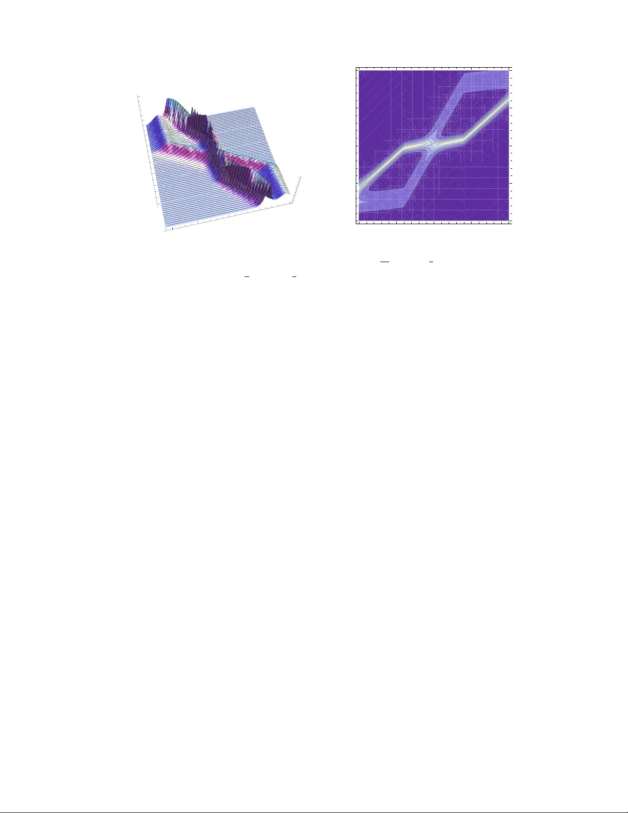
Nonautonomous mixed mKdV-sinh-Gordon hierarc h y J.F. Gomes, G. R. de Melo, L.H. Ymai and A.H. Zimerman Instituto de F ´ ısica T e´ orica-UNESP Rua Dr Ben to T eobaldo F erraz 271, Blo co I I, 01140-070, S˜ ao P aulo, Brazil Abstract The construction of a nonautonomous mixed mKdV/sine-Gordon mo del is proposed b y emplo ying an infinite dimensional affine Lie algebraic structure within the zero curv ature represen tation. A systematic construction of soliton solutions is pro vided by an adaptation of the dressing metho d which tak es in to accoun t arbitrary time dep enden t functions. A particular c hoice of those arbitrary functions provides an interesting solution describing the transition of a pure mKdV system into a pure sine-Gordon soliton. 1 In tro duction Sometime ago, the study of nonlinear effects in lattice dynamics under the influence of a weak dislo cation p oten tial has lead to a mixed mKdV/sine-Gordon equation [1]. The system was sho wn to admit m ultisoliton solutions and an infinite set of conserv ation la ws [1]. More recen tly the tw o-breather solution w as discussed in [2] in connection with the propagation of few cycle pulses (FCP) in non linear optical media. According to ref. [2] the general mKdV/sine-Gordon equation, in fact, describ es the propagation of a ultrashort optical pulses in a Kerr media. Moreo ver, it was show n in [3] that, when the ressonance frequency of atoms in the ph ysical system are well ab o ve or well b elo w the c haracteristic duration of the pulse, the propagation is describ ed b y the mKdV or sine-Gordon equations resp ectiv ely . The main ob ject of this pap er is to provide a systematic construction of soliton solutions that describ e the tr ansition b etwe en the two r e gimes , i.e. go v erned by the mKdV and sine-Gordon equations. This is accomplished b y considering the mixed in tegrable mo del prop osed in [1] with tw o arbitrary time-dep endent 1 co efficien ts. In this pap er w e show the integrabilit y of the mixed model with time dep enden t co efficien ts and that, by suitable choice of these co efficien ts as a smo oth step-type functions (as shown in figs. 1 and 3) w e obtain exact solutions for the mKdV-SG transition and hence a more realistic description of suc h phenomena. 2 Algebraic F ormalism In ref. [4] the algebraic structure of the mixed mKdV/sine-Gordon equation w as form ulated within the zero curv ature represen tation and a graded infinite dimensional Lie algebraic struc- ture as we shall no w briefly review. Consider the asso ciated G = sl (2) Lie algebra with gen- erators satisfying [ h, E ± α ] = ± 2 E ± α , [ E α , E − α ] = h and grading op erator Q = 2 λ d dλ + 1 2 h . Q decomp oses the asso ciated affine Lie algebra ˆ sl (2) into graded subspaces, ˆ G = ⊕ i G i , G 2 m = { λ m h } , G 2 m +1 = { E (2 m +1) + ≡ λ m ( E α + λE − α ) , E (2 m +1) − ≡ λ m ( E α − λE − α ) } , (1) m = 0 , ± 1 , ± 2 , . . . . In [4], a simple pro of that a mixed mKdV/sine-Gordon hierarc hy is indeed an integrable mo del follows from the zero curv ature representation of the integrable hierarc hy generated b y [ ∂ x + E (1) + + A 0 , ∂ t N + D ( N ) + D ( N − 1) + · · · D (0) + D ( − 1) ] = 0 , (2) where D ( j ) ∈ G j and A 0 = v h contains the field v ariable v = v ( x, t ). According to the subspace decomp osition (2) for N = 3 and t = t 3 whic h corresp onds to the mixed mKdV-SG equation. Let us parametrize, D (3) = a 3 E (3) + + b 3 E (3) − , D (2) = c 2 λh, D (1) = a 1 E (1) + + b 1 E (1) − , D (0) = c 0 h, D ( − 1) = a − 1 E ( − 1) + + b − 1 E ( − 1) − . (3) 2 The grade b y grade decomp osing of eqn. (2) leads to b 3 = 0 , ∂ x a 3 = 0 , c 2 = a 3 v , b 1 = 1 2 ∂ x c 2 , (4) ∂ x a 1 + 2 v b 1 = 0 , ∂ x b 1 + 2 v a 1 − 2 c 0 = 0 , (5) ∂ x a − 1 + 2 v b − 1 = 0 , ∂ x b − 1 + 2 v a − 1 = 0 , (6) together with the equation of motion ∂ x c 0 − ∂ t v − 2 b − 1 = 0 . (7) In solving eqns. (4) we find a 3 = a 3 ( t ) , b 1 = a 3 ( t ) 2 v x , c 2 = a 3 ( t ) v , (8) where a 3 ( t ) is an arbitrary function of t . In tro ducing (8) in the first eqn. (5), we obtain ∂ x a 1 + a 3 ( t ) v 2 2 ! = 0 , whic h implies that a 1 + a 3 ( t ) v 2 2 = f 1 ( t ) , where f 1 ( t ) is another arbitrary function of t . It therefore follows that a 1 = f 1 ( t ) − a 3 ( t ) v 2 2 . (9) Substituting (9) in the second eqn. (5), we get c 0 = a 3 ( t ) 4  v xx − 2 v 3  + f 1 ( t ) v . (10) Adding and subtracting eqns. (6), we obtain ∂ x a ± = ∓ 2 v a ± , (11) 3 where w e hav e denoted a ± = a − 1 ± b − 1 . Without loss of generalit y we may solv e (11) by changing the v ariable v h = − ∂ x B B − 1 = φ x h, B = e − φh , (12) whic h leads us to a ± = f − 1 ( t ) e ∓ 2 φ , where f − 1 ( t ) is another arbitrary function of t . W riting a − 1 = a + + a − 2 , b − 1 = a + − a − 2 , w e find a − 1 = f − 1 ( t ) cosh (2 φ ) , b − 1 = − f − 1 ( t ) sinh (2 φ ) . (13) Substituting (10), (12) and (13) in (7), w e finally obtain a 3 ( t ) 4  φ xxxx − 6 φ 2 x φ xx  + f 1 ( t ) φ xx − φ xt + 2 f − 1 ( t ) sinh (2 φ ) = 0 . (14) Considering f 1 ( t ) = 0, a 3 ( t ) = constant and f − 1 ( t ) = constant w e find the usual mixed mKdV/sine-Gordon equation. F or f 1 ( t ) = 0, a 3 ( t ) a giv en numerical constant 6 = 0 we recov er eqn. (10) of ref. [5]. Moreo ver for f − 1 ( t ) = 0, we reco ver equation considered in [6] with a c hoice of co efficien ts that makes the mo del integrable. W e should p oin t out that by change of co ordinates (see for instance [7]) ( x, t ) → ( ˜ x, ˜ t ) = ( x + V ( t ) , t ) where V t = f 1 ( t ) follow ed by a subsequently c hange ˜ t → T = R a 3 ( ˜ t ) d ˜ t and re-scaling f − 1 → ˜ η leads to 1 4 ( φ xxxx − 6 φ 2 x φ xx ) − φ xt + 2 ˜ η ( t ) sinh (2 φ ) = 0 . (15) Although eqn. (15) corresp onds to the equation discussed in [5] the ob ject of this pap er is to consider a class of solutions that interpolates betw een the mKdV and sine-Gordon equations. 4 This is more conv enien tly accomplished by emplo ying eqn. (14) where the t wo arbitrary func- tions a 3 ( t ) and f − 1 ( t ) (with f 1 ( t ) = 0) can b e c hosen as step-lik e limiting functions (Figs. 1 and 3) as w e shall see. 3 Construction of Soliton Solutions In order to construct, in a systematic manner, the soliton solutions of the mixed mo del let us no w recall some basic asp ects of the dressing metho d (see for instance [8]). The zero curv ature represen tation (2) implies in a pure gauge configuration, i.e., ∂ x + E + A 0 = ∂ x T T − 1 , ∂ t + D (3) + · · · D ( − 1) = ∂ t T T − 1 , (16) In particular, the v acuum is obtained by setting φ v ac = 0 1 whic h implies, ∂ x T 0 T − 1 0 = − E (1) + , ∂ t T 0 T − 1 0 = − a 3 ( t ) E (3) + − f − 1 ( t ) E ( − 1) + − f 1 ( t ) E (1) + . (17) whic h after integration yields T 0 = exp  − Z t dt 0 a 3 ( t 0 ) E (3) + − Z t dt 0 f − 1 ( t 0 ) E ( − 1) + − Z t dt 0 f 1 ( t 0 ) E (1) +  exp( − xE (1) + ) , (18) F ollo wing the dressing metho d explained in [8] and employied in [4] w e define the tau-functions τ n ≡ h λ n | B | λ n i = h λ n | T 0 g T − 1 0 | λ n i , (19) where λ n , n = 0 , 1 are fundamen tal weigh ts of the full affine Kac-Mo o dy algebra ˆ sl (2), g is a constant group element which classifies the soliton solutions and B is a zero grade group 1 F or a general member of the hierarc hy ev olving according t = t 2 n +1 , the v acuun configuration implies ∂ x T 0 T − 1 0 = − E (1) + , ∂ t 2 n +1 T 0 T − 1 0 = − a 2 n +1 ( t ) E (2 n +1) + − f − 1 ( t ) E ( − 1) + − n X k =1 f 2 k − 1 ( t ) E (2 k − 1) + . 5 elemen t con taining the ph ysical fields. In order to ensure heighest w eight representations w e no w introduce central extensions within the affine Lie algebra, characterized b y ˆ c , i.e., [ h ( n ) , E ( m ) ± α ] = ± 2 E ( n + m ) ± α , [ E ( n ) α , E ( m ) − α ] = h ( n + m ) + nδ n + m, 0 ˆ c, [ h ( n ) , h ( m ) ] = 2 nδ n + m, 0 ˆ c, and define highest w eight representations, i.e., h | λ n i = δ n, 1 | λ n i , ˆ c | λ n i = | λ n i , G i | λ n i = 0 , i > 0 , (20) n = 0 , 1. Under this affine picture the group element B acquires a cen tral term contribution, B = e − φh e − ν ˆ c . (21) In order to obtain explicit space-time dep endence from the r.h.s. of (19) w e consider the v ertex op erators, V ( γ ) = ∞ X n = −∞ ( λ n h − 1 2 ˆ cδ n, 0 ) γ − 2 n + E (2 n +1) − γ − 2 n − 1 , (22) satisfying h E (2 n +1) + , V ( γ ) i = − 2 γ 2 n +1 V ( γ ) . (23) F or a general M -soliton solution the group elemen t g in (19) is written as g = M Y j =1 e α j V ( γ j ) , (24) where α j are arbitrary constan ts. W e therefore obtain τ 0 = e − ν = h λ 0 | M Y j =1 e α j ρ j ( x,t ) V ( γ j ) | λ 0 i , τ 1 = e − φ − ν = h λ 1 | M Y j =1 e α j ρ j ( x,t ) V ( γ j ) | λ 1 i , 6 where 2 ρ j ( x, t ) = e 2 γ j x +2 γ 3 j A 3 ( t )+2 γ j F 1 ( t )+2 γ − 1 j A − 1 ( t ) , (25) A 3 ( t ) = Z dt a 3 ( t ) , F 1 ( t ) = Z dt f 1 ( t ) , A − 1 ( t ) = Z dt f − 1 ( t ) . As an illustrativ e example, we consider the one and tw o soliton cases, M = 1 , 2, where τ 1 − sol 0 = e − ν = 1 − α 1 2 ρ 1 , τ 1 − sol 1 = e − ν − φ = 1 + α 1 2 ρ 1 , (26) and τ 2 − sol 0 = e − ν = 1 − α 1 2 ρ 1 − α 2 2 ρ 2 + α 1 α 2 A 1 , 2 ρ 1 ρ 2 , τ 2 − sol 1 = e − ν − φ = 1 + α 1 2 ρ 1 + α 2 2 ρ 2 + α 1 α 2 A 1 , 2 ρ 1 ρ 2 , (27) resp ectiv ely . In order to obtain (26) and (27) where we hav e used the fact that h λ n | V ( γ ) | λ n i = δ n, 1 − 1 2 , n = 0 , 1 h λ n | V ( γ 1 ) V ( γ 2 ) | λ n i = A 1 , 2 = 1 4 γ 1 − γ 2 γ 1 + γ 2 ! 2 . The general t wo soliton solution can then b e written as φ = ln  τ 0 τ 1  = ln 1 − α 1 2 ρ 1 − α 2 2 ρ 2 + α 1 α 2 A 1 , 2 ρ 1 ρ 2 1 + α 1 2 ρ 1 + α 2 2 ρ 2 + α 1 α 2 A 1 , 2 ρ 1 ρ 2 ! , (28) while the one soliton is obtained from (28) b y setting α 2 = 0. 2 In considering a general (2 n + 1)-th member of the hierarch y , ρ j ( x, t ) = e 2 γ j x +2 γ 2 n +1 j A 2 n +1 ( t )+2 P n k =1 γ 2 k − 1 j F 2 k − 1 ( t )+2 γ − 1 j A − 1 ( t ) , A 2 n +1 ( t ) = Z dt a 2 n +1 ( t ) , F 2 k − 1 = Z dt f 2 k − 1 ( t ) . 7 4 Applications According to ref. [2] the propagation of a F CP with frequency ω on a dielectric media with c haracteristic frequency Ω, ω << Ω can b e describ ed b y the mKdV equation φ z τ + a  3 2 φ 2 τ φ τ τ + φ τ τ τ τ  = 0 , where the co ordinates z and τ corresp ond respectively to the propagation distance and retarded time, while the electric field E = φ τ . F or the case where ω >> Ω, the system is describ ed b y the sine-Gordon equation, φ z τ − b sin φ = 0 . If we now consider a dielectric media with tw o characteristic frequencies Ω 1 , Ω 2 , the case in the regime Ω 1 << ω << Ω 2 , is describ ed by the mixed mKdV-SG equation , φ z τ + a  3 2 φ 2 τ φ τ τ + φ τ τ τ τ  − b sin φ = 0 , where the t w o constan ts a and b are related to the non-linear and disp ersion prop erties of the media. In order to adapt mo del (14) to such situation, define a 3 ( t ) = − 4 aθ 1 ( t ) , f 1 ( t ) = 0 , f − 1 ( t ) = b 4 θ 2 ( t ) , re-scaling φ → i 2 φ , t → z , x → τ , eqn. (14) b ecomes a θ 1 ( z )  φ τ τ τ τ + 3 2 φ 2 τ φ τ τ  + φ z τ − b θ 2 ( z ) sin φ = 0 . (29) If w e now substitute α k → − 2 iα k , and mak e use of the identit y arctan X = 1 2 i ln  1 + iX 1 − iX  , 8 w e find that the tw o soliton solution (28) may b e written as φ = 4 arctan α 1 ρ 1 + α 2 ρ 2 1 − 4 α 1 α 2 A 1 , 2 ρ 1 ρ 2 ! , (30) where ρ j = exp  2 γ j τ + 2 γ 3 j A 3 ( z ) + 2 γ − 1 j A − 1 ( z )  , A 3 ( z ) = − 4 a Z z dz 0 θ 1 ( z 0 ) , A − 1 ( z ) = b 4 Z z dz 0 θ 2 ( z 0 ) . (31) 4.1 T ransition mKdV-SG Consider no w a dielectric media in whic h Ω 1 >> 2 γ j in the region z < z 1 and Ω 2 << 2 γ j in the region z > z 2 with z 1 > z 2 suc h that there exist an ov erlap region in whic h the media admits the tw o characteristic frequencies, Ω 2 << 2 γ j << Ω 1 . As an example to describ e such a realistic situation, w e take b oth θ 1 ( z ) and θ 2 ( z ) as step-like functions (see fig. 1) with θ 1 ( z ) = 1 2 − 1 π arctan [ β 1 ( z − z 1 )] , θ 2 ( z ) = 1 2 + 1 π arctan [ β 2 ( z − z 2 )] , where β 1 e β 2 are phenomenological parameters describing the transition b et ween the t wo medias (see fig. 1). - 10 - 5 5 10 z 0.2 0.4 0.6 0.8 1.0 Θ 1 H z L - 10 - 5 5 10 z 0.2 0.4 0.6 0.8 1.0 Θ 2 H z L Figure 1: Plots of θ 1 ( z ) and θ 2 ( z ) for β 1 = β 2 = { π 8 , π 2 , 2 π } , with z 1 = 2 and z 2 = − 2. 9 They can therefore b e integrated from (32) to yield, − 1 4 a A 3 ( z ) = z 2 − ( z − z 1 ) π arctan [ β 1 ( z − z 1 )] + 1 2 π β 1 ln h 1 + β 2 1 ( z − z 1 ) 2 i , 4 b A − 1 ( z ) = z 2 + ( z − z 2 ) π arctan [ β 2 ( z − z 2 )] − 1 2 π β 2 ln h 1 + β 2 2 ( z − z 2 ) 2 i . The β 1 , β 2 → + ∞ limit, for z 1 = z 2 = 0 corresp ond to the system gov erned b y the pure mKdV in the region z < 0 and by the pure sine-Gordon equation for z > 0. In suc h limit, we ha ve, θ 1 ( z ) = 1 2 1 − | z | z ! , θ 2 ( z ) = 1 2 1 + | z | z ! , (32) and − 1 4 a A 3 ( z ) = 1 2 ( z − | z | ) , 4 b A − 1 ( z ) = 1 2 ( z + | z | ) . (33) Figure 2 below shows the transition mKdV-SG for the one soliton solution, α 1 = 1 , α 2 = 0. The plot on the right sho ws the soliton solution view ed from the ab o v e and displays the transition (differen t velocities) from the mKdV to the SG solitons. - 5 0 5 z - 5 0 5 Τ 0 2 4 - 4 - 2 0 2 4 - 4 - 2 0 2 4 z Τ Figure 2: Plot (left) and contour plot (right) of φ τ with a = 1 10 , b = − 7 4 , β 1 = β 2 = 8 π , z 1 = 1, z 2 = − 1 and γ 1 = 14 10 . 10 4.2 T ransition mKdV-SG-mKdV Another example consist in tw o equal media separated by a second one describing, for instance the mKdV-SG-mKdV transition. Mathematically this situation may b e described b y com bining theta-t yp e functions (see fig. 3), i.e., θ 1 ( z ) = 1 − 1 π arctan h ¯ β 1 ( z − ¯ z 1 ) i + 1 π arctan h ¯ β 2 ( z − ¯ z 2 ) i , ¯ z 1 < ¯ z 2 , θ 2 ( z ) = 1 π arctan [ β 1 ( z − z 1 )] − 1 π arctan [ β 2 ( z − z 2 )] , z 1 < z 2 , with z 1 ≤ ¯ z 1 , and ¯ z 2 ≤ z 2 to guaran tee the existence of an ov erlap region b et w een the tw o medias. - 10 - 5 5 10 z 0.2 0.4 0.6 0.8 1.0 Θ H z L Figure 3: Plot of θ 1 ( z ) (dashed) and θ 2 ( z ) (con tinuum) with β 1 = β 2 = ¯ β 1 = ¯ β 2 = 8 π , z 1 = − 6, z 2 = 6, ¯ z 1 = − 4 and ¯ z 2 = 4. After in tegration (32) we find − 1 4 a A 3 ( z ) = z − ( z − ¯ z 1 ) π arctan h ¯ β 1 ( z − ¯ z 1 ) i + ( z − ¯ z 2 ) π arctan h ¯ β 2 ( z − ¯ z 2 ) i + 1 2 π ¯ β 1 ln h 1 + ¯ β 2 1 ( z − ¯ z 1 ) 2 i − 1 2 π ¯ β 2 ln h 1 + ¯ β 2 2 ( z − ¯ z 2 ) 2 i , 4 b A − 1 ( z ) = ( z − z 1 ) π arctan [ β 1 ( z − z 1 )] − ( z − z 2 ) π arctan [ β 2 ( z − z 2 )] − 1 2 π β 1 ln h 1 + β 2 1 ( z − z 1 ) 2 i + 1 2 π β 2 ln h 1 + β 2 2 ( z − z 2 ) 2 i , The limit β 1 , β 2 , ¯ β 1 , ¯ β 2 → + ∞ , when z 1 = ¯ z 1 e z 2 = ¯ z 2 with z 1 < z 2 , corresp onds to the pure mKdV case in the region z < z 1 and z > z 2 , and pure sine-Gordon in the region z 1 < z < z 2 . 11 Under suc h limiting case we hav e θ 1 ( z ) = 1 − 1 2 | z − z 1 | ( z − z 1 ) − | z − z 2 | ( z − z 2 ) ! , θ 2 ( z ) = 1 2 | z − z 1 | ( z − z 1 ) − | z − z 2 | ( z − z 2 ) ! , suc h that − 1 4 a A 3 ( z ) = z − 1 2 ( | z − z 1 | − | z − z 2 | ) , 4 b A − 1 ( z ) = 1 2 ( | z − z 1 | − | z − z 2 | ) . Figure 4 represen ts the mKdV-SG-mKdV transition for one soliton solution. - 5 0 5 z - 5 0 5 Τ 0 2 4 - 4 - 2 0 2 4 - 4 - 2 0 2 4 z Τ Figure 4: Plot (left) and contour plot (righ t) of φ τ with a = 1 10 , b = − 7 4 , β 1 = β 2 = ¯ β 1 = ¯ β 2 = 8 π , z 1 = − 4, z 2 = 4, ¯ z 1 = − 3, ¯ z 2 = 3 and γ 1 = 14 10 . 4.3 Tw o soliton solution The t wo soliton solution ( α 1 = α 2 = 1) can b e represented by As a conclusion, w e ha v e adapted the general dressing construction of soliton solutions to the mixed mKdV-SG hierarch y with arbitrary “time” dep enden t functions. The choice of such arbitrary functions as step-type functions allow ed exact solutions describing smo oth transitions from the mKdV to sine-Gordon regime and therefore more realistic mo dels. 12 - 10 - 5 0 5 10 z - 10 - 5 0 5 10 Τ 0 2 4 6 - 10 - 5 0 5 10 - 10 - 5 0 5 10 z Τ Figure 5: Plot (left) and contour plot (righ t) of φ τ with a = 1 10 , b = − 7 4 , β 1 = β 2 = ¯ β 1 = ¯ β 2 = 8 π , z 1 = ¯ z 1 = − 4, z 2 = ¯ z 2 = 4, γ 1 = 3 2 e γ 2 = 1 2 . Ac kno wledgements LHY and GRM ackno wledges supp ort from F ap esp and Cap es resp ectiv ely , JF G and AHZ thank CNPq for partial supp ort. References [1] K. Konno, W. Kameyama and H. San uki, J. of Phys. So c. of Jap an 37 (1974),171; K. Konno and H. San uki, J. of Phys. So c. of Jap an 37 (1974),292 [2] H. Leblond and D. Mihalache, Phys. Rev. A79 (2009) 063835 [3] H. Leblond and F. Sanchez, Phys. Rev. A67 (2003) 013804; H. Leblond, S.V. Sazono v, I.V. Mel’nik ov, D. Mihalache anfd F. Sanc hez, Phys. Rev. A74 (2006) 063815 [4] J.F. Gomes, G.R de Melo and A.H. Zimerman, J. Physics A42 (2009) 275208, arXiv:0903.0579 [nlin.SI] 13 [5] A. Kundu, R. Sahadev an and L. Nalinidevi, J. Ph ysics A42 (2009) 115213, nlin- Si/0811.0924 [6] K. Pradhan and P .K. Panigrahi, J. Physics A39 (2006) L343 [7] A. Kundu, Phys. Rev. E79 (2009) 015601 [8] O. Bab elon and D. Bernard, In t. J. Mo d. Ph ys. A8 (1993) 507; L. F erreira, J.L. Miramon tes and J. Sanchez-Guill ´ en, J. Math. Phys. 38 (1997) 882, arXiv:hep-th/9606066 14