A Hierarchical Latent Vector Model for Learning Long-Term Structure in Music

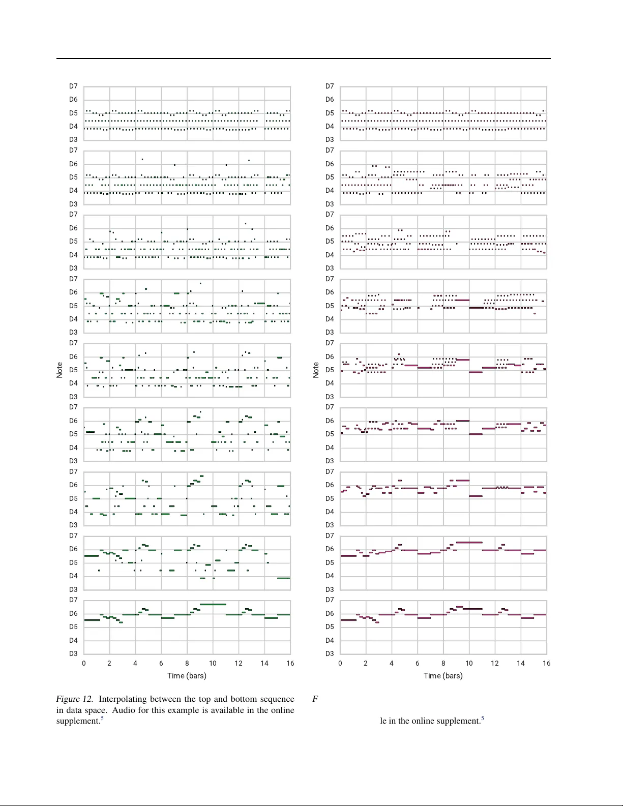
A Hierar chical Latent V ector Model f or Lear ning Long-T erm Structure in Music Adam Roberts 1 Jesse Engel 1 Colin Raffel 1 Curtis Hawthorne 1 Douglas Eck 1 Abstract The V ariational Autoencoder (V AE) has pro ven to be an effecti v e model for producing semantically meaningful latent representations for natural data. Ho wev er , it has thus far seen limited application to sequential data, and, as we demonstrate, existing recurrent V AE models have difficulty modeling sequences with long-term structure. T o address this issue, we propose the use of a hierar chical decoder , which first outputs embeddings for sub- sequences of the input and then uses these em- beddings to generate each subsequence indepen- dently . This structure encourages the model to utilize its latent code, thereby a voiding the “pos- terior collapse” problem, which remains an issue for recurrent V AEs. W e apply this architecture to modeling sequences of musical notes and find that it exhibits dramatically better sampling, inter - polation, and reconstruction performance than a “flat” baseline model. An implementation of our “MusicV AE” is av ailable online. 2 1. Introduction Generativ e modeling describes the frame work of estimating the underlying probability distrib ution p ( x ) used to generate data x . This can f acilitate a wide range of applications, from sampling novel datapoints to unsupervised representation learning to estimating the probability of an existing data- point under the learned distrib ution. Much recent progress in generativ e modeling has been expedited by the use of deep neural networks, producing “deep generativ e models, ” which lev erage the expressiv e power of deep networks to model complex and high-dimensional distrib utions. Practi- cal achiev ements include generating realistic images with 1 Google Brain, Mountain V iew , CA, USA. Correspondence to: Adam Roberts < adarob@google.com > . Pr oceedings of the 35 th International Conference on Machine Learning , Stockholm, Sweden, PMLR 80, 2018. Copyright 2018 by the author(s). 2 https://goo.gl/magenta/musicvae- code 3 https://goo.gl/magenta/musicvae- examples                         Figure 1. Demonstration of latent-space av eraging using MusicV AE. The latent codes for the top and bottom sequences are av eraged and decoded by our model to produce the middle se- quence. The latent-space mean in volv es a similar repeating pattern to the top sequence, b ut in a higher re gister and with intermittent pauses like the bottom sequence. Audio for this e xample is avail- able in the online supplement. 3 See Figs. 12 and 13 in Appendix E for a baseline comparison. millions of pixels ( Karras et al. , 2017 ), generating synthetic audio with hundreds of thousands of timesteps ( van den Oord et al. , 2016a ), and achieving state-of-the-art perfor- mance on semi-supervised learning tasks ( W ei et al. , 2018 ). A wide v ariety of methods ha ve been used in deep generati ve modeling, including implicit models such as Generati ve Adversarial Networks (GANs) ( Goodfellow et al. , 2014 ) and explicit deep autore gressive models such as Pix elCNN ( van den Oord et al. , 2016b ) and W a veNet ( van den Oord et al. , 2016a ). In this w ork, we focus on deep latent v ariable models such as the V ariational Autoencoder (V AE) ( Kingma & W elling , 2014 ; Rezende et al. , 2014 ). The advantage of these models is that the y explicitly model both p ( z | x ) and p ( z ) , where z is a latent vector that can either be inferred from existing data or sampled from a distrib ution over the A Hierarchical Latent V ector Model for Lear ning Long-T erm Structure in Music latent space. Ideally , the latent vector captures the pertinent characteristics of a giv en datapoint and disentangles factors of variation in a dataset. These autoencoders also model the likelihood p ( x | z ) , which provides an efficient way of mapping the latent vector back to the data space. Our interest in deep latent variable models primarily comes from their increasing use in creati ve applications of machine learning ( Carter & Nielsen , 2017 ; Ha & Eck , 2018 ; Engel et al. , 2017a ). This arises from surprising and con venient characteristics of the latent spaces typically learned by these models. For example, a veraging the latent codes for all datapoints that possess a given attribute produces a so-called attribute vector , which can be used to make tar geted changes to data examples. Encoding a datapoint with some attribute (say , a photograph of a person with brown hair) to obtain its latent code, subtracting the corresponding attribute v ector (the “bro wn hair” vector), adding another attribute vector (“blond hair”), and decoding the resulting latent vector can produce a realistic manifestation of the initial point with the attributes swapped (the same person with blond hair) ( Larsen et al. , 2016 ; Mikolo v et al. , 2013 ). As another example, interpolating between latent vectors and decoding points on the trajectory can produce realistic intermediate datapoints that morph between the characteristics of the ends in a smooth and semantically meaningful way . Most work on deep latent variable models has focused on continuous-valued data with a fixed dimensionality , e.g., images. Modeling sequential data is less common, partic- ularly sequences of discrete tokens such as musical scores, which typically require the use of an autoregressi ve decoder . This is partially because autoregression is often suf ficiently powerful that the autoencoder ignores the latent code ( Bow- man et al. , 2016 ). While they have shown some success on short sequences (e.g., sentences), deep latent variable models hav e yet to be successfully applied to very long sequences. T o address this gap, we introduce a nov el sequential autoen- coder with a hierarchical recurrent decoder, which helps ov ercome the aforementioned issue of modeling long-term structure with recurrent V AEs. Our model encodes an entire sequence to a single latent vector , which enables many of the creativ e applications enjoyed by V AEs of images. W e show experimentally that our model is capable of ef fectiv ely autoencoding substantially longer sequences than a baseline model with a “flat” decoder RNN. In this paper , we focus on the application of modeling se- quences of musical notes. W estern popular music exhibits strong long-term structure, such as the repetition and v ari- ation between measures and sections of a piece of music. This structure is also hierarchical–songs are divided into sections, which are broken up into measures, and then into beats, and so on. Further , music is fundamentally a multi- stream signal, in the sense that it often in volv es multiple players with strong inter -player dependencies. These unique properties, in addition to the potential creativ e applications, make music an ideal testbed for our sequential autoencoder . After cov ering a background of work our approach builds on, we describe our model and its novel architectural en- hancements. W e then provide an ov erview of related work on applying latent variable models to sequences. Finally , we demonstrate the ability of our method to model musical data through quantitativ e and qualitative e valuations. 2. Background Fundamentally , our model is an autoencoder , i.e., its goal is to accurately reconstruct its inputs. Howe ver , we addition- ally desire the ability to draw novel samples and perform latent-space interpolations and attribute vector arithmetic. For these properties, we adopt the frame work of the V aria- tional Autoencoder . Successfully using V AEs for sequences benefits from some additional extensions to the V AE objec- tiv e. In the following subsections, we cov er the prior work that forms the backbone for our approach. 2.1. V ariational A utoencoders A common constraint applied to autoencoders is that they compress the relev ant information about the input into a lower -dimensional latent code. Ideally , this forces the model to produce a compressed representation that captures im- portant factors of variation in the dataset. In pursuit of this goal, the V ariational Autoencoder ( Kingma & W elling , 2014 ; Rezende et al. , 2014 ) introduces the constraint that the latent code z is a random v ariable distributed accord- ing to a prior p ( z ) . The data generation model is then z ∼ p ( z ) , x ∼ p ( x | z ) . The V AE consists of an encoder q λ ( z | x ) , which approximates the posterior p ( z | x ) , and a decoder p θ ( x | z ) , which parameterizes the likelihood p ( x | z ) . In practice, the approximate posterior and likelihood dis- tributions (“encoder” and “decoder”) are parameterized by neural networks with parameters λ and θ respectiv ely . Fol- lowi ng the frame work of V ariational Inference, we do poste- rior inference by minimizing the KL div ergence between our approximate posterior, the encoder , and the true posterior p ( z | x ) by maximizing the evidence lo wer bound (ELBO) E [log p θ ( x | z )] − KL( q λ ( z | x ) || p ( z )) ≤ log p ( x ) (1) where the expectation is taken with respect to z ∼ q λ ( z | x ) and KL( ·||· ) is the KL-di ver gence. Naiv ely computing the gradient through the ELBO is infeasible due to the sampling operation used to obtain z . In the common case where p ( z ) is a diagonal-co variance Gaussian, this can be circumv ented by replacing z ∼ N ( µ, σ I ) with  ∼ N (0 , I ) , z = µ + σ   (2) A Hierarchical Latent V ector Model for Lear ning Long-T erm Structure in Music 2 . 1 . 1 . β - V A E A N D F R E E B I T S One way of interpreting the ELBO used in the V AE is by considering its two terms, E [log p θ ( x | z )] and KL( q λ ( z | x ) || p ( z )) , separately . The first can be thought of as requiring that p ( x | z ) is high for samples of z from q λ ( z | x ) –ensuring accurate reconstructions. The second en- courages q λ ( z | x ) to be close to the prior –ensuring we can generate realistic data by sampling latent codes from p ( z ) . The presence of these terms suggests a trade-of f between the quality of samples and reconstructions–or equi valently , be- tween the rate (amount of information encoded in q λ ( z | x ) ) and distortion (data likelihood) ( Alemi et al. , 2017 ). As is, the ELBO has no way of directly controlling this trade-off. A common modification to the ELBO introduces the KL weight hyperparameter β ( Bowman et al. , 2016 ; Higgins et al. , 2017 ) producing E [log p θ ( x | z )] − β KL( q λ ( z | x ) || p ( z )) (3) Setting β < 1 encourages the model to prioritize reconstruc- tion quality ov er learning a compact representation. Another approach for adjusting this trade-of f is to only en- force the KL regularization term once it exceeds a threshold ( Kingma et al. , 2016 ): E [log p θ ( x | z )] − max(KL( q λ ( z | x ) || p ( z )) − τ , 0) (4) This stems from the interpretation that KL( q λ ( z | x ) || p ( z )) measures the amount of information required to code sam- ples from p ( z ) using q λ ( z | x ) . Utilizing this threshold there- fore amounts to gi ving the model a certain budget of “free bits” to use when learning the approximate posterior . Note that these modified objecti ves no longer optimize a lower bound on the likelihood, but as is custom we still refer to the resulting models as “V ariational Autoencoders. ” 2 . 1 . 2 . L AT E N T S P AC E M A N I P U L A T I O N The broad goal of an autoencoder is to learn a compact rep- resentation of the data. For creati ve applications, we hav e additional uses for the latent space learned by the model ( Carter & Nielsen , 2017 ; Roberts et al. , 2018 ). First, given a point in latent space that maps to a realistic datapoint, nearby latent space points should map to datapoints that are semantically similar . By e xtrapolation, this implies that all points along a continuous curve connecting two points in latent space should be decodable to a series of datapoints that produce a smooth semantic interpolation in data space. Further , this requirement effecti vely mandates that the latent space is “smooth” and does not contain any “holes, ” i.e., isolated regions that do not map to realistic datapoints. Sec- ond, we desire that the latent space disentangles meaningful semantic groups in the dataset. Ideally , these requirements should be satisfied by a V AE if the likelihood and KL div ergence terms are both suffi- ciently small on held-out test data. A more practical test of these properties is to interpolate between points in the latent space and test whether the corresponding points in the data space are interpolated in a semantically meaningful way . Concretely , if z 1 and z 2 are the latent vectors correspond- ing to datapoints x 1 and x 2 , then we can perform linear interpolation in latent space by computing c α = αz 1 + (1 − α ) z 2 (5) for α ∈ [0 , 1] . Our goal is satisfied if p θ ( x | c α ) is a realistic datapoint for all α , p θ ( x | c α ) transitions in a semantically meaningful way from p θ ( x | c 0 ) to p θ ( x | c 1 ) as we vary α from 0 to 1, and that p θ ( x | c α ) is perceptually similar to p θ ( x | c α + δ ) for small δ . Note that because the prior ov er the latent space of a V AE is a spherical Gaussian, samples from high-dimensional priors are practically indistinguishable from samples from the uniform distribution on the unit hypersphere ( Husz ´ ar , 2017 ). In practice we therefore use spherical interpolation ( White , 2016 ) instead of Eq. ( 5 ). An additional test for whether our autoencoder will be use- ful in creati ve applications measures whether it produces reliable “attribute v ectors. ” Attribute v ectors are computed as the average latent v ector for a collection of datapoints that share some particular attrib ute. T ypically , attribute v ectors are computed for pairs of attrib utes, e.g., images of people with and without glasses. The model’ s ability to discov er attributes is then tested by encoding a datapoint with at- tribute A, subtracting the “attrib ute A vector” from its latent code, adding the “attribute B vector”, and testing whether the decoded result appears lik e the original datapoint with attribute B instead of A. In our experiments, we use the abov e latent space manipulation techniques to demonstrate the power of our proposed model. 2.2. Recurrent V AEs While a wide variety of neural network structures have been considered for the encoder and decoder network in a V AE, in the present work we are most interested in mod- els with a recurrent encoder and decoder ( Bowman et al. , 2016 ). Concretely , the encoder , q λ ( z | x ) , is a recurrent neural network (RNN) that processes the input sequence x = { x 1 , x 2 , . . . , x T } and produces a sequence of hidden states h 1 , h 2 , . . . , h T . The parameters of the distribution ov er the latent code z are then set as a function of h T . The decoder , p θ ( x | z ) , uses the sampled latent vector z to set the initial state of a decoder RNN, which autoregressi vely produces the output sequence y = { y 1 , y 2 , . . . , y T } . The model is trained both to reconstruct the input sequence (i.e., y i = x i , i ∈ { 1 , . . . , T } ) and to learn an approximate poste- rior q λ ( z | x ) close to the prior p ( z ) , as in a standard V AE. There are two main drawbacks of this approach. First, RNNs A Hierarchical Latent V ector Model for Lear ning Long-T erm Structure in Music Z ♪ ♪ ♪ ♪ ♪ ♪ ♪ ♪ ♪ 16 16 16 Encoder Latent Code Conductor Input Decoder Output Figure 2. Schematic of our hierarchical recurrent V ariational Au- toencoder model, MusicV AE. are themselves typically used on their own as powerful autoregressi ve models of sequences. As a result, the decoder in a recurrent V AE is itself sufficiently powerful to produce an ef fectiv e model of the data and may disregard the latent code. W ith the latent code ignored, the KL div ergence term of the ELBO can be tri vially set to zero, despite the fact that the model is effecti vely no longer acting as an autoencoder . Second, the model must compress the entire sequence to a single latent vector . While this approach has been shown to work for short sequences ( Bo wman et al. , 2016 ; Sutske ver et al. , 2014 ), it begins to fail as the sequence length increases ( Bahdanau et al. , 2015 ). In the follo wing section, we present a latent variable autoencoder that o vercomes these issues by using a hierarchical RNN for the decoder . 3. Model At a high le vel, our model follows the basic structure used in previously-proposed V AEs for sequential data ( Bowman et al. , 2016 ). Howe ver , we introduce a nov el hierarchical de- coder , which we demonstrate produces substantially better performance on long sequences in Section 5 . A schematic of our model, which we dub “MusicV AE, ” is shown in Fig. 2 . 3.1. Bidirectional Encoder For the encoder q λ ( z | x ) , we use a two-layer bidirectional LSTM network ( Hochreiter & Schmidhuber , 1997 ; Schus- ter & P aliwal , 1997 ). W e process an input sequence x = { x 1 , x 2 , . . . , x T } to obtain the final state vectors − → h T , ← − h T from the second bidirectional LSTM layer . These are then concatenated to produce h T and fed into two fully- connected layers to produce the latent distrib ution parame- ters µ and σ : µ = W hµ h T + b µ (6) σ = log (exp( W hσ h T + b σ ) + 1) (7) where W hµ , W hσ and b µ , b σ are weight matrices and bias vectors, respecti vely . In our experiments, we use an LSTM state size of 2048 for all layers and 512 latent dimensions. As is standard in V AEs, µ and σ then parametrize the latent distribution as in Eq. ( 2 ). The use of a bidirectional recur- rent encoder ideally gi ves the parametrization of the latent distribution longer -term context about the input sequence. 3.2. Hierarchical Decoder In prior work, the decoder in a recurrent V AE is typically a simple stacked RNN. The decoder RNN uses the latent vector z to set its initial state, and proceeds to generate the output sequence autoregressi vely . In preliminary ex- periments (discussed in Section 5 ), we found that using a simple RNN as the decoder resulted in poor sampling and reconstruction for long sequences. W e believ e this is caused by the vanishing influence of the latent state as the output sequence is generated. T o mitigate this issue, we propose a no vel hierarchical RNN for the decoder . Assume that the input sequence (and target output sequence) x can be segmented into U nonov erlapping subsequences y u with endpoints i u so that y u = { x i u , x i u +1 , x i u +2 , . . . , x i u +1 − 1 } (8) → x = { y 1 , y 2 , . . . , y U } (9) where we define the special case of i U +1 = T . Then, the latent vector z is passed through a fully-connected layer 4 follo wed by a tanh acti vation to get the initial state of a “con- ductor” RNN. The conductor RNN produces U embedding vectors c = { c 1 , c 2 , . . . , c U } , one for each subsequence. In our experiments, we use a two-layer unidirectional LSTM for the conductor with a hidden state size of 1024 and 512 output dimensions. Once the conductor has produced the sequence of embed- ding vectors c , each one is individually passed through a shared fully-connected layer followed by a tanh activ ation to produce initial states for a final bottom-layer decoder RNN. The decoder RNN then autore gressively produces a sequence of distributions ov er output tokens for each subse- quence y u via a softmax output layer . At each step of the bottom-lev el decoder, the current conductor embedding c u is concatenated with the previous output token to be used as the input. In our experiments, we used a 2-layer LSTM with 1024 units per layer for the decoder RNN. In principle, our use of an autoregressi ve RNN decoder still allo ws for the “posterior collapse” problem where the model effecti vely learns to ignore the latent state. Simliar to ( Chen et al. , 2017 ), we find that it is important to limit the scope of the decoder to force it to use the latent code to model long-term structure. For a CNN decoder, this is as simple as reducing the recepti ve field, b ut no direct analogy exists 4 Throughout, whene ver we refer to a “fully-connected layer , ” we mean a simple affine transformation as in Eq. ( 6 ). A Hierarchical Latent V ector Model for Lear ning Long-T erm Structure in Music for RNNs, which in principle hav e an unlimited temporal receptiv e field. T o get around this, we reduce the ef fectiv e scope of the bottom-le vel RNN in the decoder by only allow- ing it to propagate state within an output subsequence. As described abov e, we initialize each subsequence RNN state with the corresponding embedding passed down by the con- ductor . This implies that the only w ay for the decoder to get longer-term conte xt is by using the embeddings produced by the conductor , which in turn depend solely on the latent code. W e experimented with an autoregressi ve version of the conductor where the decoder state was passed back to the conductor at the end of each subsequence, but found it exhibited worse performance. W e believe that these com- bined constraints ef fecti vely force the model to utilize the conductor embeddings, and by e xtension the latent vector , in order to correctly autoencode the sequence. 3.3. Multi-Stream Modeling Many common sources of sequential data, such as text, consist solely of a single “stream, ” i.e., there is only one sequence source which is producing tokens. Howe ver , mu- sic is often a fundamentally multi-stream signal–a giv en musical sequence may consist of multiple players produc- ing notes in tandem. Modeling music therefore may also in volve modeling the comple x inter-stream dependencies. W e explore this possibility by introducing a “trio” model, which is identical to our basic MusicV AE except that it produces 3 separate distributions over output tokens–one for each of three instruments (drum, bass, and melody). In our hierarchical decoder model, we consider these separate streams as an orthogonal “dimension” of hierarchy , and use a separate decoder RNN for each instrument. The embed- dings from the conductor RNN initialize the states of each instrument RNN through separate fully-connected layers followed by tanh activ ations. For our baseline with a “flat” (non-hierarchical) decoder , we use a single RNN and split its output to produce per-instrument softmax es. 4. Related W ork A closely related model is the aforementioned recurrent V AE of ( Bo wman et al. , 2016 ). Like ours, their model is effecti vely a V AE that uses RNNs for both the encoder and decoder . W ith careful optimization, ( Bo wman et al. , 2016 ) demonstrate the ability to generate and interpolate between sentences which ha ve been modeled at the character le vel. A very similar model w as also proposed by ( Fabius & v an Amersfoort , 2015 ), which was applied with limited success to music. This approach was also e xtended to utilize a con- volutional encoder and decoder with dilated conv olutions in ( Y ang et al. , 2017 ). The primary difference between these models and ours is the decoder architecture; namely , we use a hierarchical RNN. The flat RNN decoder we use as a baseline in Section 5 exhibits significantly degraded performance when dealing with very long sequences. V arious additional V AE models with autoregressi ve de- coders hav e also been proposed. ( Semeniuta et al. , 2017 ) consider extensions of the recurrent V AE where the RNNs are replaced with feed-forward and con volutional networks. The PixelV AE ( Gulrajani et al. , 2017 ) marries a V AE with a PixelCNN ( van den Oord et al. , 2016b ) and applies the result to the task of natural image modeling. Similarly , the V ariational Lossy Autoencoder ( Chen et al. , 2017 ) combines a V AE with a PixelCNN/Pix elRNN decoder . The authors also consider limiting the power of the decoder and using a more expressi ve Inv erse Autoregressi ve Flo w ( Kingma et al. , 2016 ) prior on the latent codes. Another example of a V AE with a recurrent encoder and decoder is SketchRNN ( Ha & Eck , 2018 ), which successfully models sequences of continuously-valued pen coordinates. The hierarchical paragraph autoencoder proposed in ( Li et al. , 2015 ) has sev eral parallels to our work. The y also consider an autoencoder with hierarchical RNNs for the encoder and decoder , where each le vel in the hierarchy corresponds to natural subsequences in text (e.g., sentences and words). Howe ver , they do not impose any constraints on the latent code, and as a result are unable to sample or interpolate between sequences. Our model otherwise differs in its use of a flat bidirectional encoder and lack of autoregressi ve connections in the first level of the hierarchy . More broadly , our model can be considered in the sequence- to-sequence framew ork ( Sutskev er et al. , 2014 ), where an encoder produces a compressed representation of an in- put sequence which is then used to condition a decoder to generate an output sequence. For example, the NSynth model learns embeddings by compressing audio waveforms with a downsampling conv olutional encoder and then re- constructing audio with a W aveNet-style decoder ( Engel et al. , 2017b ). Recurrent sequence-to-sequence models are most often applied to sequence transduction tasks where the input and output sequences are dif ferent. Ne vertheless, sequence-to-sequence autoencoders hav e been occasion- ally considered, e.g., as an auxiliary unsupervised training method for semi-supervised learning ( Dai & Le , 2015 ) or in the paragraph autoencoder described abo ve. Again, our approach dif fers in that we impose structure on the com- pressed representation (our latent vector) so that we can perform sampling and interpolation. Finally , there hav e been many recurrent models proposed where the recurrent states are themselves stochastic latent vari ables with dependencies across time ( Chung et al. , 2015 ; Bayer & Osendorfer , 2014 ; Fraccaro et al. , 2016 ). A par- ticularly similar e xample to our model is that of ( Serban et al. , 2017 ), which also utilizes a hierarchical encoder and decoder . Their model uses tw o le vels of hierarchy and gener - A Hierarchical Latent V ector Model for Lear ning Long-T erm Structure in Music ates a stochastic latent variable for each subsequence of the input sequence. The crucial difference between this class of models and ours is that we use a single latent variable to represent the entire sequence, which allows for creati ve ap- plications such as interpolation and attribute manipulation. 5. Experiments T o demonstrate the power of the MusicV AE, we carried out a series of quantitativ e and qualitative studies on music data. First, we demonstrate that a simple recurrent V AE like the one described in ( Bowman et al. , 2016 ) can eff ec- tiv ely generate and interpolate between short sequences of musical notes. Then, we move to significantly longer note sequences, where our nov el hierarchical decoder is neces- sary in order to effecti vely model the data. T o verify this assertion, we provide quantitati ve evidence that it is able to reconstruct, interpolate between, and model attributes from data significantly better than the baseline. W e conclude with a series of listening studies which demonstrate that our proposed model also produces a dramatic impro vement in the perceiv ed quality of samples. 5.1. Data and T raining For our data source, we use MIDI files, which are a widely- used digital score format. MIDI files contain instructions for the notes to be played on each indi vidual instrument in a song, as well as meter (timing) information. W e collected ≈ 1 . 5 million unique files from the web, which provided am- ple data for training our models. W e extracted the follo wing types of training data from these MIDI files: 2- and 16-bar melodies (monophonic note sequences), 2- and 16-bar drum patterns (e vents corresponding to playing dif ferent drums), and 16-bar “trio” sequences consisting of separate streams of a melodic line, a bass line, and a drum pattern. For further details on our dataset creation process, refer to Appendix A . For ease of comparison, we also ev aluated reconstruction quality (as in Section 5.3 belo w) on the publicly av ailable Lakh MIDI Dataset ( Raffel , 2016 ) in Appendix B . W e modeled the monophonic melodies and basslines as sequences of 16th note ev ents. This resulted in a 130- dimensional output space (categorical distribution o ver to- kens) with 128 “note-on” tokens for the 128 MIDI pitches, plus single tok ens for “note-of f ” and “rest”. For drum pat- terns, we mapped the 61 drum classes defined by the General MIDI standard ( International MIDI Association , 1991 ) to 9 canonical classes and represented all possible combinations of hits with 512 categorical tokens. For timing, in all cases we quantized notes to 16th note intervals, such that each bar consisted of 16 ev ents. As a result, our two-bar data (used as a proof-of-concept with a flat decoder) resulted in sequences with T = 32 and 16-bar data had T = 256 . For our hierarchical models, we use U = 16 , meaning each subsequence corresponded to a single bar . All models were trained using Adam ( Kingma & Ba , 2014 ) with a learning rate annealed from 10 − 3 to 10 − 5 with ex- ponential decay rate 0.9999 and a batch size of 512. The 2- and 16-bar models were run for 50k and 100k gradient updates, respecti vely . W e used a cross-entropy loss against the ground-truth output with scheduled sampling ( Bengio et al. , 2015 ) for 2-bar models and teacher forcing for 16-bar models. 5.2. Short Sequences As a proof that modeling musical sequences with a recurrent V AE is possible, we first tried modeling 2-bar ( T = 32 ) monophonic music sequences (melodies and drum patterns) with a flat decoder . The model was given a tolerance of 48 free bits ( ≈ 33 . 3 nats) and had the KL cost weight, β , annealed from 0.0 to 0.2 with e xponential rate 0.99999. Scheduled sampling was introduced with an in verse sigmoid rate of 2000. W e found the model to be highly accurate at reconstruct- ing its input (T able 1 discussed below in Section 5.3 ). It was also able to produce compelling interpolations (Fig. 14 , Appendix E ) and samples. In other words, it learned to ef- fecti vely use its latent code without suf fering from posterior collapse or exposure bias, as particularly e videnced by the relativ ely small difference in teacher-forced and sampled reconstruction accuracy (a fe w percent). Despite this success, the model was unable to reliably re- construct 16-bar ( T = 256 ) sequences. For example, the discrepancy between teacher-forced and sampled reconstruc- tion accuracy increased by more than 27%. This motiv ated our design of the hierarchical decoder described in Sec- tion 3.2 . In the following sections, we pro vide an extensi ve comparison of our proposed model to the flat baseline. 5.3. Reconstruction Quality T eacher-Forcing Sampling Model Flat Hierarchical Flat Hierarchical 2-bar Drum 0.979 - 0.917 - 2-bar Melody 0.986 - 0.951 - 16-bar Melody 0.883 0.919 0.620 0.812 16-bar Drum 0.884 0.928 0.549 0.879 T rio (Melody) 0.796 0.848 0.579 0.753 T rio (Bass) 0.829 0.880 0.565 0.773 T rio (Drums) 0.903 0.912 0.641 0.863 T able 1. Reconstruction accuracies calculated both with teacher- forcing (i.e., next-step prediction) and full sampling. All values are reported on a held-out test set. A softmax temperature of 1.0 was used in all cases, meaning we sampled directly from the logits. A Hierarchical Latent V ector Model for Lear ning Long-T erm Structure in Music T o begin, we e valuate whether the hierarchical decoder pro- duces better reconstruction accurac y on 16-bar melodies and drum patterns. For 16-bar models, we giv e a tolerance of 256 free bits ( ≈ 177 . 4 nats) and use β = 0 . 2 . T able 1 shows the per-step accuracies for reconstructing the sequences in our test set. As mentioned above, we see signs of poste- rior collapse with the flat baseline, leading to reductions in accuracy of ≈ 27 − 32% when teacher forcing is removed for inference. Our hierarchical decoder both increases the next-step prediction accuracy and further reduces the ex- posure bias by better learning to use its latent code. W ith the hierarchical model, the decrease in sampling accuracy versus teacher forcing only ranges between ≈ 5 − 11% . In general, we also find that the reconstruction errors made by our models are reasonable, e.g., notes shortened by a beat or the addition of notes in the appropriate key . W e also explored the performance of our models on our multi-stream “trio” dataset, consisting of 16-bar sequences of melody , bass, and drums. As with single-stream data, the hierarchical model was able to achie ve higher accurac y than the flat baseline while e xhibiting a much smaller gap between teacher-forced and sampled performance. Figure 3. Latent-space interpolation results. All values are aver - aged ov er 1024 interpolated sequences. X-axis denotes interpola- tion between sequence A to B from left to right. T op: Sequence- normalized Hamming distance between sequence A and interpo- lated points. The distance from B is symmetric to A (decreasing as A increases) and is not shown. Bottom: Relative log probability according to an independently-trained 5-gram language model. 5.4. Interpolations For creativ e purposes, we desire interpolations that are smoothly varying and semantically meaningful. In Fig. 3 , we compare latent-space interpolations from a flat decoder (yellow circles) and hierarchical decoder (magenta squares) to a baseline of naiv e blending of the two sequences (green diamonds). W e averaged the behavior of interpolating be- tween 1024 16-bar melodies from the ev aluation dataset (A) and 1024 other unique e valuation melodies (B), using a softmax temperature of 0.5 to sample the intermediate sequences. W e constructed baseline “Data” interpolations by sampling a Bernoulli random v ariable with parameter α to choose an element from either sequence a or b for each time step, i.e., p ( x t = b t ) = α , p ( x t = a t ) = 1 − α . The top graph of Fig. 3 shows that the (sequence length- normalized) Hamming distance, i.e., the proportion of timestep predictions that dif fer between the interpolation and sequence A, increases monotonically for all methods. The data interpolation varies linearly as expected, follow- ing the mean of the Bernoulli distribution. The Hamming distances also vary monotonically for latent space interpola- tions, showing that the decoded sequences morph smoothly to be less like sequence A and more like sequence B. For example, reconstructions don’t remain on one mode for sev- eral steps and then jump suddenly to another . Samples ha ve a non-zero Hamming distance at the endpoints because of imperfect reconstructions, and the hierarchical decoder has a lower intercept due to its higher reconstruction accurac y . For the bottom graph of Fig. 3 , we first trained a 5-gram language model on the melody dataset ( Heafield , 2011 ). W e show the normalized cost for each interpolated sequence giv en by C α  ( αC B + (1 − α ) C A ) , where C α is the language model cost of an interpolated sequence with interpolation amount α , and C A and C B are the costs for the endpoint se- quences A and B . The lar ge hump for the data interpolation shows that interpolated sequences in data space are deemed by the language model to be much less probable than the original melodies. The flat model does better , but produces less coherent interpolated sequences than the hierarchical model, which produces interpolations of equal probability to the originals across the entire range of interpolation. Fig. 1 sho ws two e xample melodies and their corresponding midpoint in MusicV AE space. The interpolation synthesizes semantic elements of the two melodies: a similar repeating pattern to A, in a higher re gister with intermittent sparsity like B, and in a new shared musical ke y . On the other hand, the baseline data interpolation just mix es the two resulting in harmonic and rhythmic dissonance (Fig. 12 , Appendix E ). 5.5. Attribute V ector Arithmetic W e can also exploit the structure of the latent space to use “attribute v ectors” to alter the attributes of a gi ven sequence. Apart from the score itself, MIDI contains limited annota- tions ( Raffel & Ellis , 2016 ), so we defined five attributes which can be trivially computed directly from the note se- quence: C diatonic membership, note density , av erage in- terval, and 16th and 8th note syncopation. See Appendix C for their full definitions. Ideally , computing the dif ference A Hierarchical Latent V ector Model for Lear ning Long-T erm Structure in Music C Diatonic Density Average Interval 16th Note Syncopation 8th Note Syncopation C Diatonic Density Average Interval 16th Note Syncopation 8th Note Syncopation C Diatonic Density Average Interval 16th Note Syncopation 8th Note Syncopation > 100% 50% 0% -50% < -100% Figure 4. Adding (left) and subtracting (right) dif ferent attribute vectors in latent space and decoding the result produces the in- tended changes with few side ef fects. The vertical axis denotes the attribute vector applied and the horizontal axis denotes the attribute measured. See Figs. 6 and 8 to 11 (Appendix E ) for example piano rolls and Appendix C for descriptions of each attribute. between the a verage latent vector for sequences which e x- hibit the two e xtremes of each attribute and then adding or subtracting it from latent codes of existing sequences will produce the intended semantic manipulation. T o test this, we first measured these attributes in a set of 370k random training examples. For each attribute, we ordered the set by the amount of attribute exhibited, partitioned it into quartiles, and computed an attribute vector by subtract- ing the mean latent vector of the bottom quartile from the mean latent vector of the top quartile. W e then sampled 256 random vectors from the prior , added and subtracted vec- tors for each attribute, and measured the a verage percentage change for all attributes against the sequence decoded from the unaltered latent code. The results are sho wn in Fig. 4 . In general, we find that applying a giv en attribute vector consistently produces the intended change to the targeted attribute. W e also find cases where increasing one attribute decreases another (e.g. increasing density decreases 8th note syncopation), which we believ e is largely because our heuristics capture overlapping characteristics. W e are in- terested in e v aluating attrib ute vector manipulations for la- bels that are non-trivial to compute (e.g., ornamentation, call/response, etc.) in future work. 5.6. Listening T ests Capturing whether samples from our model sound realistic is dif ficult to do with purely quantitati ve metrics. T o com- pare the perceiv ed sample quality of the different models, we therefore carried out listening studies for melodies, trio compositions, and drum patterns. Participants were presented with two 16-bar ( ≈ 30 s) compo- sitions that were either sampled from one of the models or extracted from our e valuation dataset. They were then ask ed which they thought was more musical on a Likert scale. For each study , 192 ratings were collected, with each source                        Figure 5. Results of our listening tests. Black error bars indicate estimated standard deviation of means. Double asterisks for a pair indicate a statistically significant difference in ranking. in volved in 128 pair-wise comparisons. All samples were generated using a softmax temperature of 0.5. Fig. 5 shows the number of comparisons in which a com- position from each model was selected as more musical. Our listening test clearly demonstrates the improv ement in sample quality gained by using a hierarchical decoder–in all cases the hierarchical model was preferred dramatically more often than the flat model and at the same rate as the ev aluation data. In fact, the hierarchical drum model was preferred more often than real data, but the dif ference is not statistically significant. This was likely due to a listener bias tow ards variety , as the true drum data, while more realistic, was also more repetiti ve and perhaps less engaging. Further , a Kruskal-W allis H test of the ratings showed that there was a statistically significant dif ference between the models: χ 2 (2) = 37 . 85 , p < 0 . 001 for melodies, χ 2 (2) = 76 . 62 , p < 0 . 001 for trios, and χ 2 (2) = 44 . 54 , p < 0 . 001 for drums. A post-hoc analysis using the W ilcoxon signed- rank test with Bonferroni correction sho wed that participants rated samples from the 3 hierarchical models as more musi- cal than samples from their corresponding flat models with p < 0 . 01 / 3 . Participants also rank ed real data as more mu- sical than samples from the flat models with p < 0 . 01 / 3 . There was no significant dif ference between samples from the hierarchical models and real data. Audio of some of the examples used in the listening tests is av ailable in the online supplement. 3 6. Conclusion W e proposed MusicV AE, a recurrent V ariational Autencoder which utilizes a hierarchical decoder for improv ed modeling of sequences with long-term structure. In experiments on music data, we thoroughly demonstrated through quanti- tativ e and qualitativ e experiments that our model achie ves substantially better performance than a flat baseline. In fu- ture work, we are interested in testing our model on other types of sequential data. T o facilitate future research on recurrent latent variable models, we make our code and pre-trained models publicly av ailable. 2 A Hierarchical Latent V ector Model for Lear ning Long-T erm Structure in Music Acknowledgements The authors wish to thank David Ha for inspiration and guidance. W e thank Claire Kayacik and Cheng-Zhi Anna Huang for their assistance with the user study analysis. W e thank Erich Elsen for additional editing. References Alemi, A. A., Poole, B., Fischer , I., Dillon, J. V ., Saurous, R. A., and Murphy , K. An information-theoretic anal- ysis of deep latent-variable models. arXiv preprint arXiv:1711.00464 , 2017. Bahdanau, D., Cho, K., and Bengio, Y . Neural machine translation by jointly learning to align and translate. In Thir d International Conference on Learning Repr esenta- tions , 2015. Bayer , J. and Osendorfer , C. Learning stochastic recurrent networks. In NIPS W orkshop on Advances in V ariational Infer ence , 2014. Bengio, S., V inyals, O., Jaitly , N., and Shazeer , N. Sched- uled sampling for sequence prediction with recurrent neu- ral netw orks. In Advances in Neur al Information Pr ocess- ing Systems , 2015. Bowman, S., V ilnis, L., V inyals, O., Dai, A., Jozefo wicz, R., and Bengio, S. Generating sentences from a continuous space. In Pr oceedings of the T wentieth Conference on Computational Natural Languag e Learning , 2016. Carter , S. and Nielsen, M. Using Artificial Intelligence to Augment Human Intelligence. Distill , 2017. Chen, X., Kingma, D. P ., Salimans, T ., Duan, Y ., Dhariwal, P ., Schulman, J., Sutskev er, I., and Abbeel, P . V ariational lossy autoencoder . In F ifth International Conference on Learning Repr esentations , 2017. Chung, J., Kastner, K., Dinh, L., Goel, K., Courville, A., and Bengio, Y . A recurrent latent v ariable model for sequen- tial data. In Advances in Neural Information Pr ocessing Systems , pp. 2980–2988, 2015. Dai, A. M. and Le, Q. V . Semi-supervised sequence learning. In Advances in Neur al Information Pr ocessing Systems , 2015. Engel, J., Hoffman, M., and Roberts, A. Latent constraints: Learning to generate conditionally from unconditional generativ e models. arXiv pr eprint arXiv:1711.05772 , 2017a. Engel, J., Resnick, C., Roberts, A., Dieleman, S., Eck, D., Simonyan, K., and Norouzi, M. Neural audio synthesis of musical notes with wa venet autoencoders. In Interna- tional Confer ence on Machine Learning , 2017b. Fabius, O. and v an Amersfoort, J. R. V ariational recurrent auto-encoders. In Third International Confer ence on Learning Repr esentations , 2015. Fraccaro, M., Sønderby , S. K., Paquet, U., and Winther , O. Sequential neural models with stochastic layers. In Advances in Neural Information Pr ocessing Systems , pp. 2199–2207, 2016. Goodfellow , I., Pouget-Abadie, J., Mirza, M., Xu, B., W arde-Farley , D., Ozair , S., Courville, A., and Bengio, Y . Generati ve adversarial nets. In Advances in Neural Information Pr ocessing Systems , 2014. Gulrajani, I., Kumar , K., Ahmed, F ., T aiga, A. A., V isin, F ., V azquez, D., and Courville, A. PixelV AE: A latent variable model for natural images. In F ifth International Confer ence on Learning Representations , 2017. Ha, D. and Eck, D. Oph a neural representation of sketch drawings. In Sixth International Confer ence on Learning Repr esentations , 2018. Heafield, K. Kenlm: Faster and smaller language model queries. In Pr oceedings of the Sixth W orkshop on Statisti- cal Machine T ranslation , pp. 187–197. Association for Computational Linguistics, 2011. Higgins, I., Matthey , L., Pal, A., Burgess, C., Glorot, X., Botvinick, M., Mohamed, S., and Lerchner , A. beta- vae: Learning basic visual concepts with a constrained variational frame work. In F ifth International Confer ence on Learning Repr esentations , 2017. Hochreiter , S. and Schmidhuber, J. Long short-term memory . Neural computation , 9(8):1735–1780, 1997. Husz ´ ar , F . Gaussian distrib utions are soap bubbles. inFER- ENCe , 2017. International MIDI Association, T . General MIDI level 1 specification. 1991. Karras, T ., Aila, T ., Laine, S., and Lehtinen, J. Progres- siv e growing of gans for impro ved quality , stability , and variation. arXiv preprint , 2017. Kingma, D. P . and Ba, J. Adam: A method for stochastic op- timization. In 3rd International Confer ence on Learning Repr esentations , 2014. Kingma, D. P . and W elling, M. Auto-encoding variational bayes. In Second International Conference on Learning Repr esentations , 2014. Kingma, D. P ., Salimans, T ., Jozefowicz, R., Chen, X., Sutske ver , I., and W elling, M. Improved variational in- ference with in verse autoregressi ve flo w . In Advances in Neural Information Pr ocessing Systems , 2016. A Hierarchical Latent V ector Model for Lear ning Long-T erm Structure in Music Larsen, A. B. L., Sønderby , S. K., Larochelle, H., and W inther , O. Autoencoding beyond pix els using a learned similarity metric. In International Confer ence on Ma- chine Learning , 2016. Li, J., Luong, M.-T ., and Jurafsky , D. A hierarchical neu- ral autoencoder for paragraphs and documents. In ACL , 2015. Mikolov , T ., Sutske ver , I., Chen, K., Corrado, G. S., and Dean, J. Distributed representations of words and phrases and their compositionality . In Advances in Neur al Infor- mation Pr ocessing Systems , 2013. Raffel, C. Learning-based methods for comparing se- quences, with applications to audio-to-midi alignment and matching . PhD thesis, Columbia Uni versity , 2016. Raffel, C. and Ellis, D. P . W . Extracting ground-truth infor - mation from MIDI files: A MIDIfesto. In Pr oceedings of the 17th International Society for Music Information Retrieval Confer ence , 2016. Rezende, D. J., Mohamed, S., and W ierstra, D. Stochastic backpropagation and approximate inference in deep gen- erativ e models. In International Confer ence on Machine Learning , 2014. Roberts, A., Engel, J., Oore, S., and Eck, D. (eds.). Learning Latent Repr esentations of Music to Generate Interactive Musical P alettes , 2018. Schuster , M. and Paliwal, K. K. Bidirectional recurrent neu- ral networks. IEEE T ransactions on Signal Pr ocessing , 45(11):2673–2681, 1997. Semeniuta, S., Se veryn, A., and Barth, E. A hybrid con volu- tional v ariational autoencoder for text generation. arXiv pr eprint arXiv:1702.02390 , 2017. Serban, I. V ., Sordoni, A., Lowe, R., Charlin, L., Pineau, J., Courville, A., and Bengio, Y . A hierarchical latent variable encoder -decoder model for generating dialogues. In Thirty-F irst AAAI Confer ence on Artificial Intellig ence , 2017. Sutske ver , I., V inyals, O., and Le, Q. V . Sequence to se- quence learning with neural networks. In Advances in Neural Information Pr ocessing Systems , 2014. van den Oord, A., Dieleman, S., Zen, H., Simonyan, K., V inyals, O., Grav es, A., Kalchbrenner , N., Senior , A., and Kavukcuoglu, K. W avenet: A generati ve model for raw audio. arXiv preprint , 2016a. van den Oord, A., Kalchbrenner , N., V inyals, O., Espeholt, L., Grav es, A., and Kavukcuoglu, K. Conditional image generation with PixelCNN decoders. In Advances in Neural Information Pr ocessing Systems , 2016b. W ei, X., Liu, Z., W ang, L., and Gong, B. Improving the improv ed training of W asserstein GANs. In Sixth Inter- national Confer ence on Learning Representations , 2018. White, T . Sampling generative networks: Notes on a few effecti ve techniques. arXiv pr eprint arXiv:1609.04468 , 2016. Y ang, Z., Hu, Z., Salakhutdinov , R., and Berg-Kirkpatrick, T . Improved v ariational autoencoders for text modeling using dilated con volutions. In International Confer ence on Machine Learning , 2017. A Hierarchical Latent V ector Model for Lear ning Long-T erm Structure in Music A. Dataset Creation Details The datasets were b uilt by first searching the web for publicly-av ailable MIDI files, resulting in ≈ 1 . 5 million unique files. W e remov ed those that were identified as ha v- ing a non-4/4 time signature and used the encoded tempo to determine bar boundaries, quantizing to 16 notes per bar (16th notes). For the 2-bar (16-bar) drum patterns, we used a 2-bar (16- bar) sliding windo w (with a stride of 1 bar) to extract all unique drum sequences (channel 10) with at most a sin- gle bar of consecuti ve rests, resulting in 3.8 million (11.4 million) examples. For 2-bar (16-bar) melodies, we used a 2-bar (16-bar) slid- ing window (with a stride of 1 bar) to extract all unique monophonic sequences with at most a single bar of consec- utiv e rests, resulting in 28.0 million (19.5 million) unique examples. For the trio data, we used a 16-bar sliding windo w (with a stride of 1 bar) to extract all unique sequences containing an instrument with a program number in the piano, chromatic percussion, organ, or guitar interv al, [0, 31], one in the bass interval, [32, 39], and one that is a drum (channel 10), with at most a single bar of consecuti ve rests in any instrument. If there were multiple instruments in any of the three cat- egories, we took the cross product to consider all possible combinations. This resulted in 9.4 million examples. In all cases, we reserved a held-out ev aluation set of exam- ples which we use to report reconstruction accuracy , inter- polation results, etc. B. Lakh MIDI Dataset Results For easier comparison, we also trained our 16-bar models on the publicly a vailable Lakh MIDI Dataset (LMD) ( Raf fel , 2016 ), which makes up a subset of the our dataset described abov e. W e extracted 3.7 million melodies, 4.6 million drum patterns, and 116 thousand trios from the full LMD. The models were trained with the same hyperparameters as were used for the full dataset. W e first e valuated the LMD-trained melody model on a subset of the full ev aluation set made by excluding an y examples in the LMD train set. W e found less than a 1% difference in reconstruction accuracies between the LMD- trained and original model. In T able 2 we report the reconstruction accuracies for all 3 16-bar models trained and e valuated on LMD. While the accuracies are slightly higher than T able 1 , the same con- clusions regarding the relati ve performance of the models hold. T eacher-Forcing Sampling Model Flat Hierarchical Flat Hierarchical 16-bar Melody 0.952 0.956 0.685 0.867 16-bar Drum 0.937 0.955 0.794 0.908 T rio (Melody) 0.866 0.868 0.660 0.760 T rio (Bass) 0.906 0.912 0.651 0.782 T rio (Drums) 0.943 0.946 0.641 0.895 T able 2. Reconstruction accuracies for the Lakh MIDI Dataset calculated both with teacher-forcing (i.e., next-step prediction) and full sampling. All values are reported on a held-out test set. A softmax temperature of 1.0 was used in all cases, meaning we sampled directly from the logits. C. Attribute Definitions The following definitions were used to measure the amount of each attribute. C Diatonic The fraction of notes in the note sequence whose pitches lay in the diatonic scale on C (A-B-C-D-E-F-G, i.e., the “white keys”). Note Density The number of note onsets in the sequence divided by the total length of the sequence measured in 16th note steps. A verage Interval The mean absolute pitch interval between consecutiv e notes in a sequence. 16th Note Syncopation The fraction of (16th note) quantized note onsets landing on an odd 16th note position (1-indexed) with no note onset at the previous 16th note position. 8th Note Syncopation The fraction of (16th note) quantized note onsets landing on an odd 8th note position (1-inde xed) with no note onset at either the previous 16th or 8th note positions. D. A udio Samples Synthesized audio for all e xamples here and in the main te xt can be found in the online supplement. 5 5 https://goo.gl/magenta/musicvae- examples A Hierarchical Latent V ector Model for Lear ning Long-T erm Structure in Music E. Additional Figures and Samples Subsequent pages include additional figures, referenced from the main text. A Hierarchical Latent V ector Model for Lear ning Long-T erm Structure in Music                                                Figure 6. V arying the amount of the “Note Density” attribute vec- tor . The amount varies from -1.5 to 1.5 in steps of 0.5, with the central sequence corresponding to no attribute v ector . Audio for this example is a vailable in the online supplement. 5                                                Figure 7. Additional resamplings of the same latent code (corre- sponding to the second-to-the-bottom in Fig. 6 ). While semanti- cally similar , the specific notes vary due to the sampling in the autoregressi ve decoder . Audio for this example is a v ailable in the online supplement. 5 A Hierarchical Latent V ector Model for Lear ning Long-T erm Structure in Music                      Figure 8. Subtracting (top) and adding (bottom) the “C Diatonic” attribute v ector from the note sequence in the middle. For ease of interpretation, notes in the C diatonic scale are sho wn in white and notes outside the scale are shown in black. Audio for this example is av ailable in the online supplement. 5 A2 A3 A4 A5 A2 A3 A4 A5 Note 0 2 4 6 8 10 12 14 16 Time (bars) A2 A3 A4 A5 Figure 9. Subtracting (top) and adding (bottom) the “ A verage In- terval” attrib ute vector from the note sequence sho wn in the middle. Audio for this example is a vailable in the online supplement. 5 C4 C5 C6 C4 C5 C6 Note 0 1 2 Time (bars) C4 C5 C6 Figure 10. Subtracting (top) and adding (bottom) the “16th Note Syncopation” attribute vector from the note sequence in the middle. For ease of interpretation, only the first 2 of each sequence’ s 16 bars are shown. V ertical lines indicate 8th note boundaries. White and black indicate syncopated and non-syncopated notes, respectively . Audio for this example is a vailable in the online supplement. 5 E4 E5 E6 E4 E5 E6 Note 0 1 2 3 4 Time (bars) E4 E5 E6 Figure 11. Subtracting (top) and adding (bottom) the “8th Note Syncopation” attribute vector from the note sequence in the middle. For ease of interpretation, only the first 4 of each sequence’ s 16 bars are sho wn. V ertical lines indicate quarter note boundaries. White and black indicate syncopated and non-syncopated notes, respectiv ely . Audio for this example is av ailable in the online supplement. 5 A Hierarchical Latent V ector Model for Lear ning Long-T erm Structure in Music                                                          Figure 12. Interpolating between the top and bottom sequence in data space. Audio for this example is available in the online supplement. 5                                                          Figure 13. Interpolating between the top and bottom sequence (same as Fig. 12 ) in MusicV AE’ s latent space. Audio for this example is a vailable in the online supplement. 5 A Hierarchical Latent V ector Model for Lear ning Long-T erm Structure in Music Figure 14. Example interpolation in the 2-bar melody MusicV AE latent space. V ertical axis is pitch (from A 3 to C 8 ) and horizontal axis is time. W e sampled 6 interpolated sequences between two test-set sequences on the left and right ends. Each 2-bar sample is shown with a different background color . Audio of an extended, 13-step interpolation between these sequences is a vailable in the online supplement. 5 Figure 15. Selected example 16-bar trio sample generated by MusicV AE. Audio for this and other samples is av ailable in the online supplement. 5 .