Decentralized MPC based Obstacle Avoidance for Multi-Robot Target Tracking Scenarios

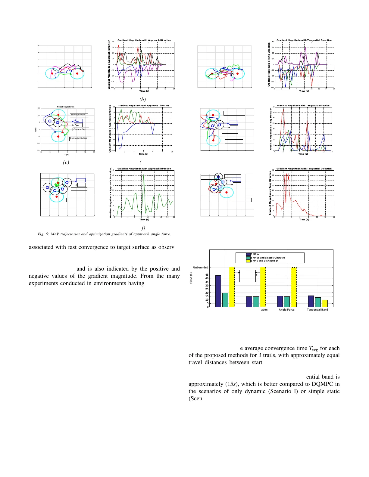
Decentralized MPC based Obstacle A v oidance for Multi-Robot T ar get T racking Scenarios Rahul T allamraju 1 , 3 , Sujit Rajappa 2 , Michael Black 1 , Kamalakar Karlapalem 3 and Aamir Ahmad 1 Abstract — In this work, we consider the problem of decentralized multi-robot target tracking and obstacle avoidance in dynamic en vironments. Each robot executes a local motion planning algorithm which is based on model predictiv e control (MPC). The planner is designed as a quadratic program, subject to constraints on robot dynamics and obstacle a voidance. Repul- sive potential field functions are employed to av oid obstacles. The novelty of our approach lies in embedding these non- linear potential field functions as constraints within a conv ex optimization framework. Our method conv exifies non-con vex constraints and dependencies, by r eplacing them as pre-computed external input forces in robot dynamics. The proposed algorithm additionally incorporates different methods to avoid field local minima problems associated with using potential field functions in planning. The motion planner does not enforce predefined trajectories or any f ormation geometry on the robots and is a comprehensiv e solution for cooperative obstacle a voidance in the context of multi-robot target tracking. Video of simulation studies: https://youtu.be/umkdm82Tt0M I . I N T RO D U C T I O N The topic of multi-robot cooperative target tracking has been researched e xtensiv ely in recent years [1]–[5]. T arget, here referes to a movable subject of interest in the environment for e.g., human, animal or other robot. Cooperativ e target tracking methods focus on impro ving the estimated pose of a tracked target while simultaneously enhancing the localization estimates of poorly localized robots, e.g., [1], by fusing the state estimate information acquired from team mate robots. The general modules inv olved in decentralized multi-robot target tracking are summarized in Fig. 1. Our work focuses on the modules related to obstacle avoidance (blue in Fig. 1). The other related modules (green in Fig. 1), such as target pose estimation, are assumed to be av ailable (see [6]). The dev eloped obstacle av oidance module fits into any general cooperativ e tar get tracking framework as seen in Fig. 1. Robots in volv ed in tracking a desired target must not collide with each other , and also with other entities (human, robot or en vironment). While addressing this problem, the state- of-art methodologies for obstacle av oidance in the context of cooperati ve target tracking ha ve drawbacks. In [7], [8] obstacle avoidance is imposed as part of the weighted MPC based optimization objective, thereby providing no guaranteed av oidance. In [1] obstacle av oidance is a separate planning module, which modifies the generated optimization trajectory using potential fields. This leads to a sub-optimal trajectory and field local minima. rahul.tallamraju, black, aamir.ahmad@tuebingen.mpg.de, sujit.rajappa@uni-tuebingen.de, kamal@iiit.ac.in 1 Perceiving Systems Department, Max Planck Institute for Intelligent Systems, T ¨ ubingen, Germany. 2 The Chair of Cognitiv e Systems, Department of Computer Science, Univ ersity of T ¨ ubingen, T ¨ ubingen, Germany. 3 Agents and Applied Robotics Group, International Institute for Information Technology , Hyderabad, India. L ow-level P osition contr oller module EKF- based Self -localization module MPC-ba sed for mation c ontr oller and obsta cle avoidanc e module T ar get P ose Detector (e.g., vision- based CNN or laser measur ements) T ar get P ose Estima tor (e.g., K alman F ilter, PF) Cooperative detec tion an d trac king modu le T ar get Detect ion measu r ements (mean + noise covarian ce mat rix) Bias cor r ection P r edicted ta r get poses T ar get pose est imate R obot Self -pose estimat e W aypoint comman ds Motion update R o b o t k + 1 R o b o t k R o b o t k - 1 T ar get Detect ion measur ements fr om teamma te r obots T eammates r obot pose estimat es Self -pose estima te + T ar get Detect ion measu r ements F ig. 1: General modules in volved in multi-r obot target tracking. Our work focuses on the modules highlighted in blue The goal of this work is to pro vide a holistic solution to the problem of obstacle avoidance, in the context of multi- robot target tracking in an en vironment with static and dy- namic obstacles. Our solution is an asynchronous and decen- tralized, model-predictive control based con vex optimization framew ork. Instead of directly using repulsive potential field functions to avoid obstacle, we con vexify the potential field forces by replacing them as pre-computed e xternal input forces in robot dynamics. As long as a feasible solution exists for the optimization program, obstacle av oidance is guaranteed. In our proposed solution we present three methods to resolve the field local minima issue. This facilitates con ver gence to a desired surface around the target. The main contributions of this work are, • Fully con vex optimization for local motion planning in the context of multi-robot target tracking • Handling non-con ve x constraints as pre-computed input forces in robot dynamics, to enforce con vexity • Guaranteed static and dynamic obstacle avoidance • Asynchronous, decentralized and scalable algorithm • Methodologies for potential field local minima av oidance Sec. II details the state-of-art methods related to obstacle av oidance, Sec. III discusses the Decentralized Quadratic Model Predictiv e Controller along with the proposed method- ologies to solve the field local minima and control deadlock problem, Sec. IV elaborates on simulation results of different scenarios, and finally we discuss future work directions. I I . S T A T E - O F - T H E - A RT The main goal in this w ork is to dev elop a decentralized multi-robot target tracker and collision free motion planner in obstacle (static and dynamic) prone environments. The multi-agent obstacle avoidance problem has gained a lot of attention in recent years. Single agent obstacle av oidance, motion planning and control is well studied [9], [10]. Ho we ver , the multi-agent obstacle a voidance problem is more complex due to motion planning dependencies between different agents, and the poor computational scalability associated with the non- linear nature of these dependencies. In general, collision free trajectory generation for multi-agents can be classified into, (i) reactiv e and, (ii) optimization based approaches. Many reacti ve approaches are based on the concept of velocity obstacle (V O) [11], whereas, optimization based approaches av oid obstacles by embedding collision constraints (like VO) within cost func- tion or as hard constraints in optimization. Recently , a mixed integer quadratic program (MIQP) in the form of a centralized non-linear model predicti ve control (NMPC) [12] has been proposed for dynamic obstacle avoidance, where feedback linearization is coupled with a variant of the branch and bound algorithm. Howe ver , this approach suf fers with agent scale-up, since increase in binary variables of MIQP has an associated exponential complexity . In general, centralized optimization approaches [13], [14] are not computationally scalable with increase in number of agents. In [15], a decentralized conv ex optimization for multi-robot collision-free formation planning through static obstacles is studied. This approach inv olves, triangular tessellation of the configuration space to con vexify static obstacle av oidance constraints. T essellated regions are used as nodes in a graph and the paths between the cells are determined to guarantee obstacle avoidance. A decentralized NMPC [16] has been proposed for pursuit e vasion and static obstacle av oidance with multiple aerial vehicles. Here the optimization is constrained by non-linear robot dynamics, resulting in non-con vexity and thereby affecting the real-time NMPC performance. Additionally , a potential field function is also used as part of a weighted objective function for obstacle av oidance. A similar decentralized NMPC has been proposed for the task of multiple UA Vs formation flight control [17]. Sequential con vex programming (SCP) has been applied to solve the problems of multi-robot collision-free trajectory gen- eration [18], trajectory optimization and tar get assignment [19] and formation payload transport [20]. These methodologies principally approximate and con ve xify the non-con vex obsta- cle av oidance constraints, and iterativ ely solve the resulting con vex optimization problem until feasibility is attained. Due to this approximation, the obtained solutions are fast within a giv en time-horizon, albeit sub-optimal. SCPs have been very effecti ve in generating real-time local motion plans with non-con vex constraints. Recent work in multi-agent obstacle av oidance [21] builds on the concept of reciprocal velocity obstacle [22], where a local motion planner is proposed to characterize and optimally choose velocities that do not lead to a collision. The approach in [21] con vexifies the velocity obstacle (V O) constraint to guarantee local obstacle avoidance. In summary , due to non-linear dynamics constraints or obsta- cle av oidance dependencies, most multi-robot obstacle avoid- ance techniques are either , (i) centralized, (ii) non-con vex, or (iii) locally optimal. Furthermore, some approaches only ex- plore the solution space partially due to constraint linearization [21]. Additionally , current NMPC target tracking approaches using potential fields do not provide guarantees on obstacle av oidance and are linked with the field local-minima problem. Recent reinforcement learning solutions [23], [24] require large number of training scenarios to determine a policy and also do not guarantee obstacle avoidance. Our work generates collision-free motion plans for each agent using a conv ex model-prediciti ve quadratic program in a decentralized manner . This approach guarantees obsta- cle avoidance and facilitates global con vergence to a target surface. T o the best of our kno wledge, the method of using tangential potential field functions [25] to generate dif ferent reactiv e swarming behaviors including obstacle av oidance, is most similar to our approach. Howe ver in [25], the field local minima is persistent in the swarming behaviors. Unlike previous NMPC based target tracking approaches, which use potential fields in the objectiv e, here we use po- tential field forces as constraints in optimization. Specifically , the non-linear potential field functions are not directly used as constraints in optimization. Instead, potential field forces are pre-computed for a horizon using the horizon motion trajectory of neighboring agents and obstacles in the vicinity . A feasible solution of the optimization program guarantees obstacle a voidance. The pre-computed values are applied as external control input forces in the optimization process thereby preserving the overall con vexity . I I I . P RO P O S E D A P P R OAC H A. Pr eliminaries W e describe the proposed framew ork for a multi-robot system tracking a desired target. For the concepts presented, we consider Micro Aerial V ehicles (MA Vs) that hover at a pre- specified height h gnd . Furthermore, we consider 2D tar get destination surface. Howe ver , the proposed approaches can be extended to any 3D surface. Let there be K MA Vs R 1 , ..., R K tracking a target x P t , typically a person P . Each MA V computes a desired destination position ˇ x R k t in the vicinity of the target position. The pose of k th MA V in the world frame at time t is giv en by ξ R k t = [( x R k t ) > ( Θ R k t ) > ] ∈ R 6 . Let there be M obstacles in the en vironment O 1 , ..., O M . The M obstacles include R k ’ s neighboring MA Vs and other obstacles in the environment. The key requirements in a multi-robot target tracking scenario are, (i) to not lose track of the moving tar get, and (ii) to ensure that the robots a void other robot agents and all obstacles (static and dynamic) in their vicinity . In order to address both these objecti ves in an integrated approach, we formulate a formation control (FC) algorithm, as detailed in Algorithm 1. The main steps have the following functionality , (i) destination point computation depending on target mov ement, (ii) obstacle av oidance force generation, (iii) decentralized quadratic model predictiv e control (DQMPC) based planner for way point generation, and (iv) a lo w-le vel position controller . T o track the waypoints generated by the MPC based planner we use a geometric tracking controller . The controller is based on the control law proposed in [26], which has a pro ven global con ver gence, aggressive maneuvering controllability and excellent position tracking performance. Here, the rota- tional dynamics controller is dev eloped directly on S O ( 3 ) and thereby av oids any singularities that arise in local coordinates. Since the MA Vs used in this work are under-actuated systems, the desired attitude generated by the outer-loop translational dynamics is controlled by means of the inner-loop torques. B. DQMPC based F ormation Planning and Control The goal of the formation control algorithm running on each MA V R k is to 1) Ho ver at a pre-specified height h gnd . 2) Maintain a distance d R k to the tracked target. 3) Orient at ya w , ψ R k , directly facing the tracked target. Additionally , MA Vs must adhere to the following constraints, 1) T o maintain a minimum distance d min from other MA Vs as well as static and dynamic obstacles. 2) T o ensure that MA Vs respect the specified state limits. 3) T o ensure that control inputs to MA Vs are within the pre-specified saturation bounds. Algorithm 1 MPC-based formation controller and obstacle av oidance by MA V R k with inputs { x P t , x O j t ; j = 1 : M } 1: { ˇ x R k t } ← Compute Destination Position { ψ R k t , x R k t , d R k , h gnd } 2: h f R k t ( 0 ) , . . . , f R k t ( N ) i ← Obstacle Force { x R k t , x O j t ( 1 : N + 1 ) , ∀ j } 3: { x R k ∗ t , ˙ x R k ∗ t , ∇ J DQM P C } ← DQMPC { ˇ x R k t , x R k t , f R k t ( 0 : N ) , g } 4: { ψ R k t + 1 } ← Compute Desired Y aw { x R k t , k ∇ J DQM P C k} 5: T ransmit x R k ∗ t ( N + 1 ) , ˙ x R k ∗ t ( N + 1 ) , ψ R k t + 1 to Low-le vel Controller Algorithm 1 outlines the strategy used by each MA V R k at ev ery discrete time instant t . In line 1, MA V R k computes its desired position ˇ x R k t on the desired surface using simple trigonometry . For example, if the desired surface is a circle, centered around the target location x P t with a radius d R k = const an t ∀ R k , then the desired position for time instant t is giv en by ˇ x R k t = x P t + h d R k cos ( ψ R k t ) d R k sin ( ψ R k t ) h gnd i > . Here ψ R k t is the yaw of R k w .r .t. the target. It is important to note that the distance d R k is an input to the DQMPC and is not necessarily the same for each MA V . In line 2, an input potential field force vector h f R k t ( 0 ) , . . . , f R k t ( N ) i > ∈ R 3 × ( N + 1 ) is computed for a planning horizon of ( N + 1 ) discrete time steps by using the shared trajectories from other MA Vs and positions of obstacles in the vicinity . If no trajectory information is av ailable, the instantaneous position based potential field force v alue is used for the entire horizon. Section III-C details the numerical computation of these field force vectors. In line 3, an MPC based planner solves a con ve x opti- mization problem (DQMPC) for a planning horizon of ( N + 1 ) discrete time steps. W e consider nominal accelerations [ u R k t ( 0 ) · · · u R k t ( N )] > ∈ R 3 × ( N + 1 ) as control inputs to DQMPC. The accelerations describe the 3D translational motion of R k . u R k t ( n ) = ¨ x R k t ( n ) (1) where n is the current horizon step. The state vector of the discrete-time DQMPC consists of R k ’ s position x R k t ( n ) ∈ R 3 and velocity ˙ x R k t ( n ) ∈ R 3 . The optimization objective is, J DQMPC =  N ∑ n = 0  Ω Ω Ω i ( u R k t ( n ) + f R k t ( n ) + g g g ) 2  + Ω Ω Ω t  h x R k t ( N + 1 ) > ˙ x R k t ( N + 1 ) > i − h ( ˇ x R k t ) > 0 > i  2  (2) The optimization is defined by the follo wing equations. x ( 1 ) R k ∗ t . . . x ( N + 1 ) R k ∗ t , u R k ∗ t ( 0 ) . . . u R k ∗ t ( N ) = arg min u R k t ( 0 ) ... u R k t ( N ) ( J DQM P C ) (3) subject to, h x R k t ( n + 1 ) > ˙ x R k t ( n + 1 ) > i > = A h x R k t ( n ) > ˙ x R k t ( n ) > i > + B ( u R k t ( n ) + f R k t ( n ) + g g g ) , (4) u min ≤ u R k t ( n ) ≤ u max , (5) x min ≤ x R k t ( n ) ≤ x max , (6) ˙ x min ≤ ˙ x R k t ( n ) ≤ ˙ x max (7) where, Ω Ω Ω i and Ω Ω Ω t are positiv e definite weight matrices for input cost and terminal state (computed desired position ˇ x R k t and desired velocity ˙ ˇ x R k t = 0) respectiv ely , f R k t ( n ) is the pre- computed external obstacle force, g g g is the constant gra vity vector . The discrete-time state-space evolution of the robot is giv en by (4). The dynamics ( A ∈ R 3 × 3 ) and control transfer ( B ∈ R 3 × 3 ) matrices are given by , A =  I 3 ∆ t I 3 0 3 I 3  , B =  ∆ t 2 2 I 3 ∆ t I 3  . (8) where, ∆ t is the sampling time. The quadratic program gener- ates optimal control inputs h u R k t ( 0 ) · · · u R k t ( N ) i and the corre- sponding trajectory h x R k t ( 1 ) ˙ x R k t ( 1 ) · · · x R k t ( N + 1 ) ˙ x R k t ( N + 1 ) i tow ards the desired position. The final predicted position and velocity of the horizon x R k ∗ t ( N + 1 ) , ˙ x R k ∗ t ( N + 1 ) is used as desired input to the low-le vel flight controller . The MPC based planner av oids obstacles (static and dynamic) through pre-computed horizon potential force f R k t ( n ) . This force is applied as an external control input component to the state- space ev olution equation, thereby , preserving the optimization con vexity . Pre vious methods in literature consider non-linear potential functions within the MPC formulation, thereby , mak- ing optimization non-conv ex and computationally e xpensiv e. In the next step (line 4 of Algorithm 1), the desired yaw is computed as ψ R k t + 1 = at an 2  y P t − y R k t x P t − x R k t  . This describes the angle with respect to the target position x P t from the MA V’ s current position x R k t . The way-point commands consisting of the position and desired yaw angle are sent to the low-le vel flight position controller . Although no specific robot formation geometry is enforced, the DQMPC naturally results in a dynamic formation depending on desired destination surface. C. Handling Non-Conve x Collision A voidance Constraints In our approach, at an y gi ven point there are two forces acting on each robot, namely (i) the attractive force due to the optimization objectiv e (eq.(3)), and (ii) the repulsive force due to the potential field around obstacles ( f R k t ( n ) ). In general, a repulsiv e force can be modeled as a force vector based on the distance w .r .t. obstacles. Here, we hav e considered the potential field force variation as a hyperbolic function ( F R k , O j hy p ( d ( n )) ) of distance between MA V R k and obstacle O j . W e use the formulation in [27] to model F R k , O j hy p ( d ( n )) . Here, Obstacle Field Target Surface Target Field Local Minima / Control Deadlock (a) F ield local minima pr oblem ⍵ R 1 ⍵ R 2 || ∇ J R 1 DQMPC || || ∇ J R 2 DQMPC || || ∇ J R 2 DQMPC || > || ∇ J R 1 DQMPC || ⇒ ⍵ R 2 > ⍵ R 1 Target Surface Target (b) Swivelling Robot Destination Method. || ∇ J R 1 DQMPC || || ∇ J R 2 DQMPC || || ∇ J R 2 DQMPC || > || ∇ J R 1 DQMPC || ⇒ F R 2 ang > F R 1 ang F R 2 ang F R 1 ang R 1 R 2 Target Surface Target (c) Appr oach Angle Method Target Surface Tangential Force Band Repulsive Force Tangential Force Resultant Force Target Obstacle R 1 R 1 R 1 path towards destination Hyperbolic Potential Field (d) T angential Band Method F ig. 2: Illustration of the field local minima pr oblem in obstacle avoidance and differ ent proposed methods. d ( n ) = k x R k t − 1 ( n ) − x O j t ( n ) k 2 , ∀ n ∈ [ 0 , . . . , N ] is the distance between the MA V’ s predicited horizon positions from the previous time step ( t − 1 ) and the obstacles (which includes shared horizon predictions of other MA Vs). The repulsi ve force vector is, F F F R k , O j re p ( n ) = ( F R k , O j hy p ( d ( n )) α , if d ( n ) < d sa f e 0 , if d ( n ) > d sa f e , (9) where, d sa f e is the distance from the obstacle where the potential field magnitude is non-zero. α = x O j t ( n ) − x R k t − 1 ( n ) k x O j t ( n ) − x R k t − 1 ( n ) k 2 is the unit vector in the direction away from the obstacle. Additionally we consider a distance d min << d sa f e around the obstacle, where the potential field magnitude tends to infinity . The potential force acting on an agent per horizon step n is, f R k t ( n ) = ∑ ∀ j F R k , O j re p ( n ) , (10) which is added into the system dynamics in eq.(4). D. Resolving the F ield Local Minima Pr oblem The key challenge in potential field based approaches is the field local minima issue [28]. When the summation of attractiv e and repulsiv e forces acting on the robot is a zero vector , the robot encounters field local minima problem 1 . Equiv alently , a control deadlock could also arise when the robot is constantly pushed in the e xact opposite direction. Both local minima and control deadlock are undesirable scenarios. From equation (4) and Algorithm 1, it is clear that the optimization can characterize control inputs that will not lead to collisions, but, cannot characterize those control inputs that lead to these scenarios. In such cases the gradient of opti- mization would be non-zero indicating that the robot knows its direction of motion towards the target, but cannot reach the destination surface because the potenial field functions are not directly used in DQMPC constraints. Here, we propose three methodologies for field local minima avoidance. 1) Swivelling Robot Destination (SRD) method: This method is based on the idea that the MA V destination ˇ x R k t is an e xternal input to the optimization. Therefore, each MA V can change its ˇ x R k t to push itself out of field local minima. For example, consider the scenario shown in Fig. 2(a), where three robots are axially aligned to wards the tar get. Since the angles of 1 note that this is dif ferent from optimization objective’ s local minima. approach are equal, the desired destination positions are the same for R 1 and R 2 , i.e., ˇ x R 1 t = ˇ x R 2 t . This results in temporary deadlock and will slow the conv ergence to desired surface. W e construct the SRD method to solve this deadlock problem as follows: (i) the gradient of DQMPC objective of R k is computed, (ii) a swiv elling velocity ω R k is calculated based on the magnitude of gradient, and (iii) ˇ x R k t swiv els by a distance proportional to ω R k as shown in Fig.2(b). This ensures that the v elocities at which each ˇ x R k t swiv els is dif ferent until the robot reaches the target surface, where the gradient tends to zero. The gradient of the optimization with respect to the last horizon step control and state vectors, is computed as follo ws. ∂ J DQM P C x R k t ( N + 1 ) = 2 Ω Ω Ω t ( h x R k t ( N + 1 ) > ( ˙ x R k t ( N + 1 )) > i − h ( ˇ x R k t ) > 0 > i ) > ∂ J DQM P C u R k t ( N ) = 2 Ω Ω Ω i ( u R k t ( n ) + f R k t ( n ) + g g g ) + 2 Ω Ω Ω t B ( x R k t ( N + 1 ) − ˇ x R k t ) ∇ J R k DQM P C = ∂ J DQM P C x R k t ( N + 1 ) + ∂ J DQM P C u R k t ( N ) . (11) For circular target surface, the destination point swiv el rate is, ˇ x R k t = x P t +    d R k cos ( ψ R k t ± k s k ∇ J R k DQM P C k ) d R k sin ( ψ R k t ± k s k ∇ J R k DQM P C k ) h gnd    > (12) where, k s is a user -defined gain controlling the impact of k ∇ J R k DQM P C k . The swiv el direction of each R k is decided by its approach direction to target. Positive and negativ e ψ R k t leads to a clockwise and anti-clockwise swivel respectively . 2) Appr oach Angle T owards T ar get Method: In this method, the local minima and control deadlock is addressed by includ- ing an additional potential field function which depends on the approach angle of the robots towards the target. Here, we (i) compute the approach angle of robot R k w .r .t. the target, (ii) compute the gradient of the objectiv e, and (iii) compute a force F R k , O j ang in the direction normal to the angle of approach, as shown in Fig. 2(c). The magnitude of F R k , O j ang depends on the sum of gradients ∇ J R k DQM P C and the hyperbolic function (see Sec. III-C) between the approach angles of robot R k and obstacles O j w .r .t. the target. This potential field force is computed as, F R k , O j ang ( n ) = ∇ J R k DQM P C F R k , O j hy p (( θ R k ( n ) − θ O j ( n )) 2 ) ˆ β ∀ j (13) β = ± x R k t ( n ) − ˇ x R k t k x R k t ( n ) − ˇ x R k t k 2 ; ˆ β . β = 0 . (14) Here θ R k ( n ) and θ O j ( n ) are the angles of R k and obstacle O j with respect to the target. The angles θ O j ∀ j w .r .t target are computed by each R k , as part of the force pre-computation using O j ’ s position. β and ˆ β are the unit vectors in the approach direction to the target and its orthogonal respecti vely , with ± dependent on θ R k w .r .t. the target. The f R k t ( n ) for n t h horizon step is therefore f R k t ( n ) = ∑ ∀ j F R k , O j re p ( n ) + F R k , O j ang ( n ) . (15) Notice that the non-linear constraint of the two approach angles not being equal is con verted into an equiv alent con- ve x constraint using pre-computed force v alues. This method ensures collision avoidance in the presence of obstacles and fast con vergence to the desired tar get, because the net potential force direction is always away from the obstacle. 3) T angential Band Method: The pre vious methods at times, do not facilitate target surface con vergence because of field local minima and control deadlock. For example, static obsta- cles forming a U-shaped boundary between the target surface and R k ’ s position, as shown in Fig.2(d). If the target surface is smaller than the projection of the static obstacle along the direction of approach to the desired surface, the planned trajectory is occluded. Therefore, the SRD method cannot find a feasible direction for motion. Furthermore, angle of approach field acts only when the θ R k and θ O j are equal w .r .t. the target. In order to resolve this, we construct a band around each obstacle where an instantaneous (at n = 0) tangential force acts about the obstacle center . The width of this band is > ( ˙ x > max ∆ t + u max ∆ t 2 2 ) and therefore, the robot cannot tunnel out of this band within one time step ∆ t . This makes sure that once the robot enters tangential band, it exits only after it has overcome the static obstacles. The direction depends on R k ’ s approach towards the target, resulting in clockwise or anti-clockwise force based on − ve or + ve value of ψ R k t respectiv ely . The outer surface of the band has only the tan- gential force effect, while the inner surface has both tangential and repulsiv e force (repulsive hyperbolic field) effects on R k . W ithin the band the diagonal entries of the positive definite weight matrix Ω Ω Ω t are reduced to a very low v alue ( ≺≺ Ω t , max ). This ensures that the attraction field on the robot is reduced while it is being pushed a way from the obstacle. Consequently , the effect of tangential force is higher in the presence of obstacles. Once the robot is out of the tangential field band (i.e., clears the U-shaped obstacles), the high weight of the Ω Ω Ω t is restored and the robot con verges to its desired destination. Fig. 2(d) illustrates this method. The tangential force is, F R k , O j t ang ( 0 ) = k t ang ∇ J R k DQM P C ˆ α , (16) where k t ang is user-defined gain and ˆ α is defined s.t. ± ˆ α . α = 0. The weight matrix and step horizon potential are therefore, Ω Ω Ω t = Ω Ω Ω t , min , if x R k t ≤ d ( 0 ) + d band (17) -15 -10 -5 0 5 10 15 X (m) -15 -10 -5 0 5 10 15 Y (m) Robot Trajectories (a) 0 5 1 0 1 5 2 0 2 5 3 0 3 5 4 0 4 5 T i me (s ) 0 1 0 2 0 3 0 4 0 5 0 6 0 G r a d i e n t M a g n i tu d e O b j e c ti v e G r a d i e n t (b) -15 -10 -5 0 5 10 15 X (m) -15 -10 -5 0 5 10 15 Y (m) Robot Trajectories Destination Surface Starting Surface d min d safe Obstacle Field (c) 0 5 1 0 1 5 2 0 2 5 3 0 3 5 T i me (s ) 0 5 1 0 1 5 2 0 2 5 3 0 3 5 4 0 4 5 G r a d i e n t M a g n i tu d e O b j e c ti v e G r a d i e n t (d) -15 -10 -5 0 5 10 15 X (m) -15 -10 -5 0 5 10 15 Y (m) Robot Trajectories Starting Surface d min d safe Obstacle Field Destination Surface (e) 0 2 4 6 8 1 0 1 2 T i me (s ) 0 5 1 0 1 5 2 0 2 5 G r a d i e n t M a g n i tu d e O b j e c ti v e G r a d i e n t (f) F ig. 3: MA V trajectories and optimization gradients of baseline DQMPC optimization. The colors (r ed, gr een, blue, black, ma genta) r epr esent R k s and their r espective gradients. f R k t ( n ) = ∑ ∀ j F R k , O j re p ( n ) + F R k , O j t ang ( 0 ) , (18) where d band is the tangential band width. The values of the weights can vary between Ω Ω Ω t , min ≺ Ω Ω Ω t ≺ Ω Ω Ω t , max and changes only when the robot is within the influence of tangential field of any obstacle. In summary , the tangential band method not only guarantees collision a voidance for any obstacles but also facilitates robot con vergence to the target surface. In rare scenarios, e.g., when the static obstacle almost encircles the robots and if the desired target surface is beyond such an obstacle, the robots could get trapped in a loop within the tangential band. This is because a minimum attraction field towards the tar get always exists. Since in this work, the objectiv e is local motion planning in dynamic environments with no global information and map, we do not plan for a feasible trajectory out of such situations. I V . R E S U L T S A N D D I S C U S S I O N S In this section, we detail the experimental setup and the results of our DQMPC based approach along with the field local minima resolving methods proposed in Sec. III for obstacle av oidance and reaching the target surface. A. Experimental Setup The algorithms were simulated in a Gazebo+ROS integrated en vironment to emulate the real world physics and enable a decentralized implementation for validation of the proposed methods. The setup runs on a standalone Intel Xeon E5-2650 processor . The simulation environment consists of multiple -15 -10 -5 0 5 10 15 X (m) -15 -10 -5 0 5 10 15 Y (m) Robot Trajectories (a) 0 2 4 6 8 1 0 1 2 1 4 T i me (s ) − 4 0 − 2 0 0 2 0 4 0 G r a d i e n t M a g n i tu d e x S w i v e l D i r e c ti on G r a d i e n t M a g n i tu d e w i th S w i v e l D i r e c ti on (b) -15 -10 -5 0 5 10 15 X (m) -15 -10 -5 0 5 10 15 Y (m) Robot Trajectories Starting Surface Destination Surface d min d safe Obstacle Field (c) 0 2 4 6 8 1 0 1 2 1 4 1 6 1 8 T i me (s ) − 5 0 − 4 0 − 3 0 − 2 0 − 1 0 0 1 0 G r a d i e n t M a g n i tu d e x S w i v e l D i r e c ti on G r a d i e n t M a g n i tu d e w i th S w i v e l D i r e c ti on (d) -15 -10 -5 0 5 10 15 X (m) -15 -10 -5 0 5 10 15 Y (m) Robot Trajectories d min d safe Starting Surface Obstacle Field Destination Surface (e) 0 2 4 6 8 1 0 1 2 1 4 1 6 1 8 T i me (s ) − 5 0 5 1 0 1 5 2 0 2 5 G r a d i e n t M a g n i tu d e x S w i v e l D i r e c ti on G r a d i e n t M a g n i tu d e w i th S w i v e l D i r e c ti on (f) F ig. 4: MA V trajectories and optimization gradients of swivelling destination method. hexarotor MA Vs confined in a 3D world of 20 m × 20 m × 20 m . All the experiments were conducted using multiple MA Vs for 3 different task scenarios in volving simultaneous target tracking and obstacle avoidance namely , • Scenario I: 5 MA Vs need to tra verse from a starting surface to destination surface without collision. Each agent acts as a dynamic obstacle to every other MA V . • Scenario II: 2 MA Vs hover at certain height and act as static obstacles. The remaining 3 MA Vs need to reach the desired surface av oiding static and dynamic obstacles. • Scenario III: 4 MA Vs hover and form a U-shaped static obstacle. The remaining MA V must reach destination while av oiding field local minima and control deadlock. It may be noted that in all the above scenarios, the target’ s position is drastically changed from initial to final destination. This is done so as to create a more challenging target tracking scenario than simple target position transitions. Furthermore, the scalability and effecti veness of the proposed algorithms are verified by antipodal position swap of 8 MA Vs within a surface. The MA Vs perform 3D obstacle av oidance to reach their respectiv e positions while ensuring that the surface center (target) is always in sight. The conv ex optimization (3)-(7) is solved as a quadratic program using CVXGEN [29]. The DQMPC operates at a rate of 100 Hz. The state and velocity limits of each MA V R k are [ − 20 , − 20 , 3 ] > ≤ x R k t ( n ) ≤ [ 20 , 20 , 10 ] > in m and [ − 5 , − 5 , − 5 ] > ≤ ˙ x R k t ( n ) ≤ [ 5 , 5 , 5 ] > in m / s respecti vely , while the control limits are [ − 2 , − 2 , − 2 ] > ≤ u R k t ( n ) ≤ [ 2 , 2 , 2 ] in m / s 2 . The desired hovering height of each MA V is h gnd = 5 m and the yaw ψ R k of each MA V is oriented towards the target. The horizon N for the DQMPC and potential force computa- tion is 15 time steps each. It is important to mention that if no trajectory information is av ailable for an obstacle or adversary O j , the n = 0 magnitude of potential field ( F R k , O j re p ( 0 ) ) is used for the entire horizon. d min = 0 . 5 m and d sa f e = 3 m for the potential field around obstacles. The destination surface is circular , with radius d R k = 4 m ∀ k , around the target for all experiments. Ho wev er , as stated earlier our approach can attain any desired 3D destination surf ace. B. DQMPC: Baseline Method Figure 3 showcases the multi-robot target tracking results for the three different scenarios (see Sec. IV -A) while applying the baseline DQMPC method. As clearly seen in Fig. 3(a,c), the agents find obstacle free trajectories from starting to destination surface for the scenarios I and II. This is also indicated by the magnitude of gradient dropping close to 0 after 40 s and 30 s respectiv ely as seen in Fig. 3(b,d). The rapidly varying gradient curve of Scenario I (Fig. 3(b)) shows that, each agent’ s potential field pushes other agents to reach the destination surface 2 . W e observe that the MA Vs conv erge to the destination (Fig. 3(c)) by a voiding the obstacle fields. In the U-shaped static obstacle case (scenario III), the agent is stuck because of control deadlock and fails to reach the destination surface as seen in Fig. 3(e). The periodic pattern of the gradient curve (Fig. 3(f)) and non-zero gradient magnitude makes the deadlock situation evident. Most of these scenarios can also be visualized in the attached video submission. C. Swivelling Robot Destination Method In the swivelling destination method, we use k s = 0 . 05 as the gain for gradient magnitude impact. Fig. 4(a) shows, the MA Vs spreading themselves along the destination surface depending on their distance from target and therefore the gradient. This method has a good con vergence time of about 12 s and 15 s (about 3 times faster than the baseline DQMPC) for the scenarios I and II as can be observed in Fig. 4(b) and Fig. 4(d) respectively . Here, the direction of swi vel depends on the agents orientation w .r .t. to target and each agent takes a clockwise or anti-clockwise swiv el based on its orientation as clearly seen in Fig. 4(c). The positiv e and negati ve v alues of the gradient indicate the direction. It can be observed in Fig. 4(c), that the agent at times crosses over the d sa f e because of the higher target attraction force but respects the d min where the repulsion force is infinite. Despite the better con vergence time, the MA V is stuck when encountered with a U-shaped static obstacle (Fig. 4(e)) because of a control deadlock. This can also be observed with the non-zero gradient in Fig. 4(f). D. Appr oach Angle T owards T ar get Method Figure 5 showcases the results of the approach angle method. Since the additional potential field force enforces that not more than one agent has the same approach angle, the MA Vs spread themselves while approaching the destination surface. This is 2 Note that the scale of the gradient plots are different. The magnitude of the gradient is just to suggest that the robot has reached the target surface. -15 -10 -5 0 5 10 15 X (m) -15 -10 -5 0 5 10 15 Y (m) Robot Trajectories (a) 0 2 4 6 8 1 0 1 2 1 4 T i me (s ) − 4 0 − 3 0 − 2 0 − 1 0 0 1 0 2 0 3 0 4 0 G r a d i e n t M a g n i tu d e x A p p r oa c h D i r e c ti on G r a d i e n t M a g n i tu d e w i th A p p r oa c h D i r e c ti on (b) -15 -10 -5 0 5 10 15 X (m) -15 -10 -5 0 5 10 15 Y (m) Robot Trajectories Destination Surface Starting Surface Obstacle Field d safe d min (c) 0 2 4 6 8 1 0 1 2 T i me (s ) − 5 0 − 4 0 − 3 0 − 2 0 − 1 0 0 1 0 2 0 3 0 G r a d i e n t M a g n i tu d e x A p p r oa c h D i r e c ti on G r a d i e n t M a g n i tu d e w i th A p p r oa c h D i r e c ti on (d) -15 -10 -5 0 5 10 15 X (m) -15 -10 -5 0 5 10 15 Y (m) Robot Trajectories Starting Surface Destination Surface d min d safe Obstacle Field (e) 0 2 4 6 8 1 0 1 2 1 4 1 6 1 8 T i me (s ) 0 5 1 0 1 5 2 0 2 5 3 0 3 5 4 0 4 5 G r a d i e n t M a g n i tu d e x A p p r oa c h D i r e c ti on G r a d i e n t M a g n i tu d e w i th A p p r oa c h D i r e c ti on (f) F ig. 5: MA V trajectories and optimization gradients of appr oach angle for ce. associated with fast conv ergence to target surface as observed in Fig. 5(a,b,c,d), for the scenarios I and II. The direction of the approach angle depends on the orientation of the MA Vs w .r .t. to the target and is also indicated by the positiv e and negati ve values of the gradient magnitude. From the many experiments conducted in en vironments having only dynamic obstacles or sparsely spaced static obstacles, we observed that this method has the smoothest transition to the destination surface. Ho wever , similar to the swi velling destination method, it also fails to o vercome control deadlock in case of a U-shaped obstacle as observed in Fig. 5(e,f). E. T angential Band Method The MA Vs using tangential band method reach the destination surface in all the scenarios of static and dynamic obstacles as seen in Fig. 6. This method f acilitates con vergence to the target, for complex static obstacles, because, by principle the MA V traverses within the band until it finds a feasible path tow ards the tar get surface. k t ang = 2 was used in simulations. As seen in Fig. 6(e), as soon as the MA V reaches obstacle surface, the tangential force acts, pushing it in the anti- clockwise direction. Then the UA V travels within this band until it is finally pulled towards the destination surface. The same principle applies for dynamic obstacles scenarios (see Fig. 6(a,c)) as well. Fig. 6(f) shows that, since the MA V over - comes field local minima and control deadlock, the gradient reaches 0 for the U-shaped obstacle with a con vergence time of 12 seconds. -15 -10 -5 0 5 10 15 X (m) -15 -10 -5 0 5 10 15 Y (m) Robot Trajectories (a) 0 2 4 6 8 1 0 1 2 1 4 1 6 T i me (s ) − 4 0 − 3 0 − 2 0 − 1 0 0 1 0 2 0 3 0 4 0 G r a d i e n t M a g n i tu d e x T a n g D i r e c ti on G r a d i e n t M a g n i tu d e w i th T a n g e n ti a l D i r e c ti on (b) -15 -10 -5 0 5 10 15 X (m) -15 -10 -5 0 5 10 15 Y (m) Robot Trajectories d min d safe Obstacle Field Destination Surface Starting Surface (c) 0 2 4 6 8 1 0 1 2 1 4 T i me (s ) 0 5 1 0 1 5 2 0 2 5 3 0 3 5 4 0 G r a d i e n t M a g n i tu d e x T a n g D i r e c ti on G r a d i e n t M a g n i tu d e w i th T a n g e n ti a l D i r e c ti on (d) -15 -10 -5 0 5 10 15 X (m) -15 -10 -5 0 5 10 15 Y (m) Robot Trajectories Starting Surface Destination Surface d min d safe Obstacle Field (e) 0 2 4 6 8 1 0 1 2 1 4 T i me (s ) 0 5 1 0 1 5 2 0 2 5 3 0 3 5 4 0 4 5 G r a d i e n t M a g n i tu d e x T a n g D i r e c ti on G r a d i e n t M a g n i tu d e w i th T a n g e n ti a l D i r e c ti on (f) F ig. 6: MA V trajectories and optimization gradients of tangential band method. Average Convergence Time DQMPC Baseline Swivel Destination Angle Force Tangential Band 0 5 10 15 20 25 30 35 40 45 Unbounded Time (s) 5 MAVs 3 MAVs and a Static Obstacle 1 MAV and U Shaped Static Obstacle Approach Fails to Converge F ig. 7: A verag e con ver gence time comparison. F . Con ver gence T ime Comparison Figure 7 compares the av erage con ver gence time T cvg for each of the proposed methods for 3 trails, with approximately equal trav el distances between starting and destination surface for the different scenarios mentioned in Sec. IV -A. The T cvg for swiv elling destination, approach angle and tangential band is approximately (15 s ), which is better compared to DQMPC in the scenarios of only dynamic (Scenario I) or simple static (Scenario II) obstacles. In the U-shaped obstacle (Scenario III), except tangential band the other methods get stuck in field local minima. It may be noted that all the method can be gen- eralized for any shape of the destination surface. In summary , the tangential band method w ould be the most preferred choice when the type of obstacles in en vironment are unkno wn. All the mentioned results and additional experimental results can also be observed in the enclosed video file. -15 -10 -5 0 5 10 15 X (m) -15 -10 -5 0 5 10 15 Y (m) Robot Trajectories -15 -10 -5 0 5 10 15 X (m) -15 -10 -5 0 5 10 15 Y (m) Robot Trajectories (a) Approach angle method (b) T angential band method T ABLE I: Robot trajectories during antipodal position swapping. G. Antipodal Movement In order to further emphasize the ef ficacy of tangential band and approach angle methods, we demonstrate obstacle a void- ance for a task of intra-surface antipodal position swapping. Here 8 MA Vs start on a circular surface with a radius of 8 m , at equal angular distance from each other w .r .t. the center (world frame origin [ 0 , 0 , 0 ] > ). The MA Vs must reach a point 180 o in the opposite direction while simultaneously maintaining their orientation towards the center . The plot in T ab. I (a) shows the trajectories taken by MA Vs in this task using the approach angle method. All the MA Vs conv ergence to their antipodal positions in around T cvg = 13 s . It may be noted that there is no trajectory specified and the MA Vs compute their own optimal motion plans. T o improve the conv ergence time in this scenario, a consistent clockwise direction is enforced, but this is not necessary and con ver gence is guaranteed either w ay . The video attachment visually showcases this antipodal mov ement. Similarly the antipodal position swapping was carried out using the tangential band method with the same experimental criteria (see figure in T ab. I (b)). A con ver gence time of around T cvg = 11 s was observed, further emphasizing the speed of obstacle av oidance and conv ergence of the proposed method. V . C O N C L U S I O N S A N D F U T U R E W O R K In this work, we successfully address the problem of obstacle av oidance in the context of decentralized multi-robot target tracking. Our algorithm uses conv ex optimization to find collision free motion plans for each robot. W e con ve xify the obstacle av oidance constraints by pre-computing the potential field forces for a horizon and using them as external force inputs in optimization. W e show that non-linear dependencies could be conv erted into such external forces. W e validate three methods to avoid field local minima by embedding external forces into the conv ex optimization. W e showcase the efficac y of our approach through gazebo+R OS simulations for vari- ous scenarios. Future work in volves physically validating the proposed methodology using multiple real robots on different robot platforms (aerial and ground). A C K N O W L E D G M E N T S The authors would like to thank Eric Price and Prof. Andreas Zell for their valuable advice during the course of this work. R E F E R E N C E S [1] P . Lima, A. Ahmad, and et al., “Formation control driven by cooperativ e object tracking, ” Robotics and Autonomous Systems , vol. 63, 2015. [2] S. S. Dias and M. G. Bruno, “Cooperative target tracking using decen- tralized particle filtering and rss sensors, ” IEEE T ransactions on Signal Pr ocessing , vol. 61, no. 14, pp. 3632–3646, 2013. [3] A. Ahmad, G. Lawless, and P . Lima, “ An online scalable approach to unified multirobot cooperative localization and object tracking, ” IEEE T ransactions on Robotics , vol. 33, no. 5, pp. 1184–1199, 2017. [4] K. Hausman and et al., “Cooperativ e control for target tracking with onboard sensing, ” in Experimental Robotics . Springer , 2016. [5] M. Zhang and H. H. Liu, “Cooperative tracking a moving target using multiple fixed-wing uavs, ” Journal of Intelligent & Robotic Systems , vol. 81, no. 3-4, pp. 505–529, 2016. [6] E. Price, G. Lawless, H. H. B ¨ ulthoff, M. Black, and A. Ahmad, “Deep neural network-based cooperati ve visual tracking through multiple micro aerial vehicles, ” arXiv preprint , 2018. [7] T . P . Nascimento and et al., “Nonlinear model predictive formation control: An iterative weighted tuning approach, ” Journal of Intelligent & Robotic Systems , vol. 80, no. 3-4, pp. 441–454, 2015. [8] T . P . Nascimento, A. G. Conceic ¸ ao, and A. P . Moreira, “Multi-robot nonlinear model predictive formation control: the obstacle av oidance problem, ” Robotica , vol. 34, no. 3, pp. 549–567, 2016. [9] M. Hoy , A. S. Matveev , and A. V . Savkin, “ Algorithms for collision-free navigation of mobile robots in complex cluttered en vironments: a surve y , ” Robotica , vol. 33, no. 3, pp. 463–497, 2015. [10] Y . Liu, S. Rajappa, and et al., “Robust nonlinear control approach to nontrivial maneuvers and obstacle av oidance for quadrotor uav under disturbances, ” Robotics and Autonomous Systems , vol. 98, 2017. [11] P . Fiorini and Z. Shiller, “Motion planning in dynamic environments using v elocity obstacles, ” The International Journal of Robotics Resear ch , vol. 17, no. 7, pp. 760–772, 1998. [12] H. Fukushima, K. K on, and F . Matsuno, “Model predicti ve formation control using branch-and-bound compatible with collision avoidance prob- lems, ” IEEE T ransactions on Robotics , v ol. 29, 2013. [13] A. U. Raghunathan and et al., “Dynamic optimization strategies for three- dimensional conflict resolution of multiple aircraft, ” Journal of guidance, contr ol, and dynamics , vol. 27, no. 4, pp. 586–594, 2004. [14] A. Kushle yev , D. Mellinger, C. Po wers, and V . Kumar , “T owards a swarm of agile micro quadrotors, ” Autonomous Robots , vol. 35, 2013. [15] J. C. Derenick and J. R. Spletzer , “Conve x optimization strategies for co- ordinating large-scale robot formations, ” IEEE T ransactions on Robotics , vol. 23, no. 6, pp. 1252–1259, 2007. [16] D. H. Shim, H. J. Kim, and S. Sastry , “Decentralized nonlinear model predictiv e control of multiple flying robots, ” in CDC , vol. 4. IEEE, 2003. [17] Z. Chao, L. Ming, Z. Shaolei, and Z. W enguang, “Collision-free uav formation flight control based on nonlinear mpc, ” in ICECC . IEEE, 2011. [18] F . Augugliaro, A. P . Schoellig, and R. D’Andrea, “Generation of collision- free trajectories for a quadrocopter fleet: A sequential conv ex program- ming approach, ” in IROS . IEEE, 2012, pp. 1917–1922. [19] D. Morgan, S.-J. Chung, and F . Y . Hadaegh, “Swarm assignment and tra- jectory optimization using variable-swarm, distrib uted auction assignment and model predictiv e control, ” in AIAA , 2015, p. 0599. [20] J. Alonso-Mora, S. Baker , and D. Rus, “Multi-robot navigation in forma- tion via sequential con vex programming, ” in IROS . IEEE, 2015. [21] J. Alonso-Mora and et al., “Collision av oidance for aerial v ehicles in multi- agent scenarios, ” Autonomous Robots , vol. 39, no. 1, pp. 101–121, 2015. [22] J. V an Den Berg, S. J. Guy , M. Lin, and D. Manocha, “Reciprocal n-body collision av oidance, ” in Robotics resear ch . Springer , 2011, pp. 3–19. [23] Y . F . Chen, M. Liu, M. Everett, and J. P . How , “Decentralized non- communicating multiagent collision avoidance with deep reinforcement learning, ” in Robotics and Automation (ICRA), 2017 IEEE International Confer ence on . IEEE, 2017, pp. 285–292. [24] P . Long, W . Liu, and J. Pan, “Deep-learned collision avoidance policy for distributed multiagent na vigation, ” IEEE Robotics and Automation Letters , vol. 2, no. 2, pp. 656–663, 2017. [25] D. E. Chang and et al., “Collision avoidance for multiple agent systems, ” in CDC , vol. 1. IEEE, 2003, pp. 539–543. [26] T . Lee, M. Leoky , and N. H. McClamroch, “Geometric tracking control of a quadrotor uav on se (3), ” in CDC . IEEE, 2010, pp. 5420–5425. [27] C. Secchi, A. Franchi, H. H. B ¨ ulthoff, and P . R. Giordano, “Bilateral con- trol of the degree of connectivity in multiple mobile-robot teleoperation, ” in Robotics and Automation (ICRA), 2013 IEEE International Conference on . IEEE, 2013, pp. 3645–3652. [28] Y . Koren and J. Borenstein, “Potential field methods and their inherent limitations for mobile robot navigation, ” in ICRA . IEEE, 1991. [29] J. Mattingley and S. Boyd, “Cvxgen: A code generator for embedded con vex optimization, ” Optimization and Engineering , vol. 13, 2012.