A Nonlocal InSAR Filter for High-Resolution DEM Generation from TanDEM-X Interferograms

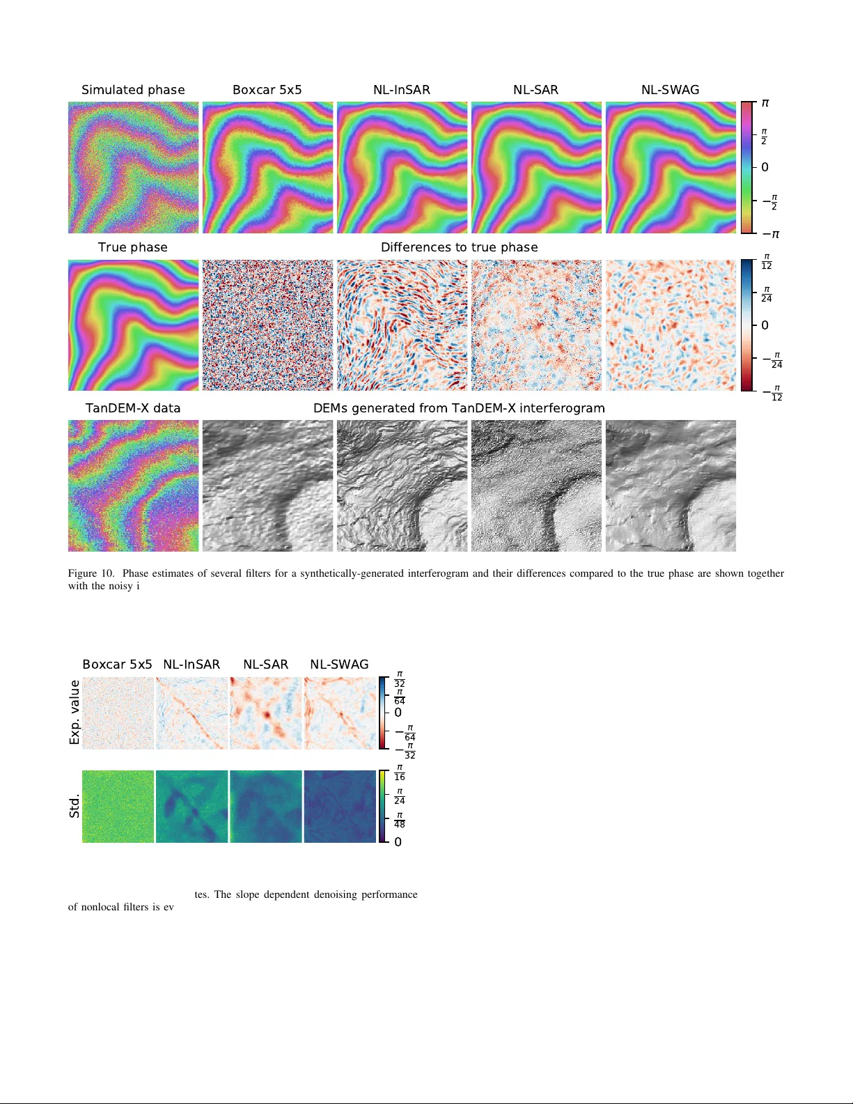
IEEE TRANSA CTIONS ON GEOSCIENCE AND REMO TE SENSING, IN PRESS 1 A Nonlocal InSAR Filter for High-Resolution DEM Generation from T anDEM-X Interferograms Gerald Baier , Cristian Rossi, Marie Lachaise, Xiao Xiang Zhu Senior Member , IEEE , Richard Bamler F ellow , IEEE Abstract — This is a preprint, to read the final v ersion please go to IEEE T ransactions on Geoscience and Remote Sensing on IEEE XPlore. This paper presents a nonlocal InSAR filter with the goal of generating digital elevation models of higher resolution and accuracy from bistatic T anDEM-X strip map interferograms than with the processing chain used in production. The currently employed boxcar multilooking filter naturally decreases the resolution and has inherent limitations on what level of noise reduction can be achieved. The proposed filter is specifically designed to account for the inher ent div ersity of natural terrain by setting several filtering parameters adaptively . In particular , it considers the local fringe frequency and scene heterogeneity , ensuring pr oper denoising of interferograms with considerable underlying topography as well as urban areas. A comparison using synthetic and T anDEM-X bistatic strip map datasets with existing InSAR filters shows the effectiveness of the proposed techniques, most of which could r eadily be integrated into existing nonlocal filters. The resulting digital elevation models outclass the ones produced with the existing global T anDEM-X DEM processing chain by effectively increasing the resolution from 12 m to 6 m and lowering the noise level by roughly a factor of two. Index T erms —digital elevation model (DEM), interferometric synthetic aperture radar (InSAR), nonlocal filtering I . I N T R O D U C T I O N W ith the global av ailability of the digital ele v ation model (DEM) produced by the German Aerospace Center’ s (DLR) T anDEM-X mission, topographic data with so far nonexistent spatial resolution and height accuracy hav e become accessible on a global scale. The fact that a complete satellite mission was set in motion and ex ecuted for this sole purpose shows the demand and need for such data. Even more attention This work is supported by the European Research Council (ERC) under the European Union’ s Horizon 2020 research and innov ation programme (grant agreement no. ERC-2016-StG-714087, acronym: So2Sat, www .so2sat.eu) and the Helmholtz Association under the framew ork of the Y oung Investig ators Group “SiPEO" (VH-NG-1018, www .sipeo.bgu.tum.de). ( Corr esponding Author: Xiao Xiang Zhu ) G. Baier is with the Remote Sensing T echnology Institute, German Aerospace Center , 82234 W essling, Germany (e-mail: gerald.baier@dlr .de). C. Rossi is with Satellite Applications Catapult, Harwell Campus, Didcot, O X11 0QR, United Kingdom. M. Lachaise is with the Remote Sensing T echnology Institute, German Aerospace Center , 82234 W essling, Germany . X. X. Zhu is with the Remote Sensing T echnology Institute, German Aerospace Center , 82234 W essling, Germany , and also with the Signal Processing for Earth Observation (SiPEO), T echnical Uni versity of Munich, 80333 Munich, German y . (e-mail: xiao.zhu@dlr .de) R. Bamler is with the Remote Sensing T echnology Institute, German Aerospace Center , 82234 W essling, Germany , and also with the Institute for Remote Sensing T echnology , T echnical Univ ersity of Munich, 80333 Munich, Germany . should be paid not to compromise resolution and accuracy after acquisition by imperfect processing steps. Phase denoising is a mandatory step within any InSAR DEM production workflo w . A more accurate phase estimate results not only in a less noisy DEM but also eases phase unwrapping. Indiscriminate spatial av eraging of the phase, also called boxcar multilooking, while being fast to compute and reducing the variance of the estimate, degrades resolution. T o address this issue, more advanced filtering methods have been the topic of research for more than two decades. Lee’ s sigma filter and its later extensions [1 – 3] are examples of SAR and polarimetric SAR filters that include statistical tests for selecting pixels in the a veraging process. Nonlocal filters were first introduced for denoising optical images [4]. In recent years, the hav e become increasingly popular within the denoising community , due to their unsur - passed noise reduction and detail preservation. The foundation of their performance is a highly discriminate search for statis- tically homogeneous pixels, somewhat akin to the sigma filter , within a large area during the filtering process. These features sparked research into adapting them to new domains, such as denoising regular SAR amplitude images [5–7], interfero- grams [8, 9], polarimetric SAR [10], and a unified approach for SAR amplitude images, interferograms and polarimetric SAR images [11]. Recent publications applied the nonlocal filtering paradigm to SAR stacks in the fields of differential SAR interferometry [12] and 3D reconstruction using SAR tomography [13]. The first nonlocal InSAR filter [8] piqued our interest to produce DEMs from bistatic T anDEM-X strip map interferograms with improv ed resolution and accuracy compared to boxcar multilooking, which is employed in DLR’ s processing chain for the global T anDEM-X DEM. For the original operational processing chain [14 – 16], the need to cope with the data volume of the global DEM acquis- tion imposed sev ere design restrictions due to computational costs. Boxcar multilooking was finally chosen, as the resulting DEM fulfills the T anDEM-X accuracy requirements [17] and its computational costs are negligible compared to the other processing steps. Our research was moti vated by the need for e ven higher- resolution DEMs which led DLR to commence research on the high-resolution DEM (HDEM) product, with increased hori- zontal resolution and vertical accuracy ov er selected areas [18] compared to the default T anDEM-X DEM product. HDEMs rely on sev eral new acquisitions with larger baselines resulting in smaller height errors from phase noise. For comparison, the heights of ambiguity for HDEM range from 10 m to 20 m IEEE TRANSA CTIONS ON GEOSCIENCE AND REMO TE SENSING, IN PRESS 2 whereas the v alues for the regular DEM start at 35 m and go up to 50 m . Thus, a boxcar averaging phase filter with a smaller spatial extent compared to the default processing toolchain suffices to fulfill the vertical accuracy goal and more of the original spatial resolution can be preserved. T able I giv es the specifications of the two available DEM products from DLR. Our goal was to create a DEM similar in accuracy to the HDEM specifications by reprocessing the acquisitions made for the global T anDEM-X DEM. The findings of our earlier in vestigation [19, 20] suggest that the qualities of nonlocal filters do indeed transfer to DEM generation. W e were able to produce a RawDEM, the initial DEM product used for creating the final T anDEM-X DEM, with 6 m × 6 m resolution sho wing more details and less noise compared to the operational product with a resolution of 12 m × 12 m . Y et our straightforward application of NL-InSAR, the non- local filter introduced in [8], led to undesired terrace-like artifacts in the final DEM. W e also found, that the more recently published NL-SAR filter [11] was unsuitable for DEM generation as it showed a tendency for oversmoothing. This paper further elaborates on the issues we encountered when applying the nonlocal filtering paradigm to InSAR denoising and proposes a ne w nonlocal InSAR filter that takes these into consideration. A key feature is its compensation of the deterministic, topographic phase component, which hampers the search for statistically homogeneous pixels in mountainous terrain. It further factors in the div ersity of natural terrain by using a local scene heterogeneity measure to select key filtering parameters instead of relying on a global, fixed set. These techniques can readily be integrated into ex- isting nonlocal InSAR filters to also bolster their performance. A comparison with a LiD AR DEM giv es an impression of and quantifies the lev el of improvement that can be achiev ed by employing nonlocal filters instead of con ventional filters to real data. Concerning the vastly increased computational cost, with the advances in semiconductor manufacturing processes and computing architecture, especially graphics processing units (GPUs), large-scale nonlocal filtering of SAR interferograms is no wadays feasible [22]. The paper is structured as follo ws. Section II briefly in- troduces the nonlocal filtering concept with respect to SAR interferometry . The design decisions of the proposed filter are described in Section III and are backed up by the experiments in Section IV. W e discuss the impact of the new filter in Sec- tion V and conclude together with an outlook in Section VI. I I . N O N L O C A L I N S A R F I LT E R I N G What sets nonlocal filters apart from other filters is the large area they operate ov er for denoising each pixel. This area, called the search windo w , is inspected for similar pix els. Their absolute position does not influence the later filtering process, true to their name “nonlocal”, unlike with many conv entional neighborhood filters. For detecting similar pixels, nonlocal filters do not only rely on comparing the pixel value alone, but also take their surrounding areas, henceforth referred to as patches, into account. By doing so, textures, structures and features help identifying similar pixels and influence the (a) Search window (blue square) and patches (green squares) (b) Similarity map Figure 1. The nonlocal filtering process: Inside the search window (blue square) centered at the pixel that is to be filtered (a), all pixels are checked for their similarity by comparing their surrounding patches to the center patch (green squares). The corresponding similarity map (b) shows that similar pixels are located along the edge. filtering results to a far larger degree than with conv entional filters. Fig. 1 illustrates this filtering process, where, in order to denoise the pixel marked by the red cross, all pixels inside the search window (blue square) are considered by comparing their surrounding patches to the center pixel’ s patch (all as green squares). The resulting similarity map is depicted on the right and sho ws that the most similar pixels are located along the edge. In the original version of the nonlocal filter, the Euclidean distance between patches was used as a measure of similarity . This measure is the least square estimate for additi ve white Gaussian noise, a common and practical model for optical images. As the noise characteristics of SAR profoundly differ , the earlier referenced filters for SAR, InSAR and polarimetric SAR all define similarity criteria depending on the statistics of the observed quantities: the speckle noise for SAR amplitude images, the interferometric phase for InSAR, or the cov ariance matrix for (Pol)(In)SAR. The patch dissimilarities ∆ in the search window are mapped into weights w by a kernel. In most cases, an exponential kernel or a slight adaption thereof is used w = e − ∆ h , (1) where h sets the trade-of f between filtering strength and detail preservation. In the following, we assume that the weights are normalized to sum to one. The estimate of an image z , in our case the interferogram z = u 1 ¯ u 2 = A 1 A 2 e j ϕ = | z | e j ϕ (2) of the master and slav e images, at the pixel location x is computed as the weighted mean ov er the corresponding search window ∂ x ˆ z x = X y ∈ ∂ x w x , y z y . (3) IEEE TRANSA CTIONS ON GEOSCIENCE AND REMO TE SENSING, IN PRESS 3 T able I R E SO LU T I O N A N D AC CU R AC Y R E QU IR EM E N T S O F T H E S TA N DA R D G LO BA L T A N D EM - X D E M A N D T H E L O CA LLY A VAI LA B L E H D E M [ 2 1] . Independent pixel spacing Absolute horizontal and Relativ e vertical accuracy vertical accuracies ( 90 % ) ( 90 % linear point-to-point) (global) T anDEM-X DEM 12 m ( 0 . 4 00 at equator) 10 m 2 m (slope ≤ 20 % ) 4 m (slope > 20 % ) (local) T anDEM-X HDEM 6 m ( 0 . 2 00 at equator) 10 m goal: 0 . 8 m ( 90 % random height error) The argument ˆ ϕ = 6 ˆ z of ˆ z is the estimate of the true interferometric phase θ . In a similar fashion, estimates of the intensity ˆ I x = X y ∈ ∂ x w x , y | u 1 , y | 2 + | u 2 , y | 2 2 (4) and coherence ˆ γ x =    P y ∈ ∂ x w x , y u 1 , y ¯ u 2 , y    q P y ∈ ∂ x w x , y | u 1 , y | 2 P y ∈ ∂ x w x , y | u 2 , y | 2 (5) can be obtained. One can think of the nonlocal filter as a selector for statistically homogeneous pixels for the av eraging process. When dealing with SAR images and InSAR images in particular , there are sev eral additional factors to consider when applying the nonlocal filter paradigm. The next section highlights these pitfalls and describes ho w they are addressed specifically by the proposed method. I I I . P R O P O S E D F I LT E R In the following, we will refer to the proposed method as NL-SW AG, short for N on L ocal- S AR interferogram filter for w ell-performing A ltitude Map G eneration. Figure 2 shows a high-lev el flow graph of NL-SW A G. The following paragraphs describe in greater detail the individual operations and how they af fect the filtering performance and outcome. W e hav e highlighted in gray operations that are explicitly explained in the respectiv ely named subsections, which will also cover other related blocks. A. Aggr egation A common filtering artifact of nonlocal filters is the so- called rar e patch effect , which occurs when only few similar patches are located within the search window , resulting in subpar filtering performance. The problem is especially prev a- lent near edges, as Fig. 1 illustrates, where for all patches that include the edge only few similar patches are found. Aggregating multiple estimates is one approach to counter this behavior [23]. Instead of the traditional pixel-wise nonlocal means filter as in Eq. (3), NL-SW A G computes the patch-wise weighted mean 2 SLCs pr e fi lter ed interfer ogram 1st st age weight computa tion phase model fi nal fi lter ed interfer ometric phase 2nd st age phase cor r ection weight computa tion fringe fr equenc y estimation patch size selection phase heter ogeneity analysis aggr egation patch -wise weighted mea n computa tion of equivalent number of looks patch -wise weighted mea n aggr egation computa tion of equivalent number of looks Figure 2. Flow graph of the proposed filter. Blocks that are highlighted in gray have their own respecti ve subsections, which will also cover other related operations. The second stage uses the prefiltered output of the first stage for computing a ne w , more reliable set of weights. ˆ z x = X y ∈ ∂ x w x , y z y . (6) The ov erlapping patch estimates ˆ z are then aggregated into a single pixel estimate, weighted by their equiv alent number of looks L ˆ z x = P y ∈P x L y ˆ z y , x − y P y ∈P x L y , (7) where P x denotes the set of all pixel indices within a patch centered at x and x − y being the relativ e index inside the respectiv e patch, i.e., z y , x − y = z x . IEEE TRANSA CTIONS ON GEOSCIENCE AND REMO TE SENSING, IN PRESS 4 The weighting by L ensures that patch estimates with a higher number of looks, and therefore a smaller variance, hav e a larger impact on the final estimate. The effecti ve number of looks, i.e., the variance reduction of the weighted mean, can directly be computed from the weight map [8] L x =  P y ∈ ∂ x w x , y  2 P y ∈ ∂ x w 2 x , y . (8) Aggregation mitigates the rare patch effect as it also properly denoises pixels near features, such as edges, as long as the y also belong to patches which do not contain said features. B. T wo Stage Filtering SAR interferograms are affected by speckle and suffer from phase noise due to the innate coherence loss between two acquisitions, rendering the similarity estimates difficult and hereby degrading the denoising performance. A solution that is often employed is a two-stage ap- proach [11, 24, 25], where in the first step the so-called guidance image is generated by prefiltering the input image. In the second step, the guidance image is used to compute the patch similarities, which can now be more reliably estimated due to the reduced noise le vel. The stages of NL-SW AG, which are also depicted in Fig. 2, employ the two similarity criteria derived in [8] for two single look complex images (SLC) in the first stage and a filtered interferogram in the second stage. 1) F irst stage: The similarity of two pixels in the first stage is the conditional likelihood of observing u i, x and u i, y ( i = 1 , 2 ), given that the true parameters, the coherence γ , the intensity I and the interferometric phase θ are identical [8]: p ( u 1 , x , u 1 , y , u 2 , x , u 2 , y | I x = I y , θ x = θ y , γ x = γ y ) = δ 1 x , y = r B C 3 A + C A r C A − C − arcsin r C A ! , (9) where A =  A 2 1 , x + A 2 2 , x + A 2 1 , y + A 2 2 , y  2 , B = A 1 , x A 2 , x A 1 , y A 2 , y and C = 4  A 2 1 , x A 2 2 , x + A 2 1 , y A 2 2 , y + 2 B cos ( ϕ x − ϕ y )  . The patch similarity in the first stage is computed as ∆ 1 x , y = X o ∈O log δ 1 x + o , y + o , (10) where O denotes the set of all index of fsets in the patch. The dissimilarities are mapped into weights by an e x- ponential kernel as in Eq. (1). As the purpose is only to reduce the noise lev el and remov e outliers without introducing sev ere filtering artifacts before computing the similarities in the second step h is set to a comparati vely small value. Except for the aggregation step, the first stage is identical to the non- iterativ e version of NL-InSAR and its guidelines for picking h can be used. The estimates of the phase, intensity and coherence are obtained via Eq. (3), Eq. (4) and Eq. (5) together with the aggregation in Eq. (6) and Eq. (7). 2) Second stage: The second stage computes the simi- larities as a function of the coherence ˆ γ , intensity ˆ I and interferometric phase ˆ ϕ estimates produced by the first stage. The symmetric Kullback-Leibler di ver gence of two zero-mean complex circular Gaussian distributions, the underlying joint distribution of ˆ γ , ˆ I and ˆ ϕ , is given by [8] δ 2 x , y = 4 π " ˆ I x ˆ I y 1 − ˆ γ x ˆ γ y cos( ˆ ϕ x − ˆ ϕ y ) 1 − ˆ γ 2 y + ˆ I y ˆ I x 1 − ˆ γ y ˆ γ x cos( ˆ ϕ y − ˆ ϕ x ) 1 − ˆ γ 2 x − 2 # (11) and can be used as a similarity criterion. Instead of a fixed patch size, the second stage changes the patch size adaptiv ely based on the local heterogeneity . The exact patch similarity and weight computation are covered in the following two sections since, as can be seen from Fig. 2, it is based on other operations. Even though the two-step approach alleviates the problems caused by the high noise level in SAR images, we hav e to stress that a repeated application of any filter can potentially introduce staircase-like artifacts in the filtered output as we observed with NL-InSAR. T o elaborate a little further: Just like traditional neighbor - hood filters, nonlocal filters can also be seen as diffusion filters [26]. Diffusion filters have the interesting property that their repeated application steadily decreases the noise le vel and produces piecewise constant approximations of the original data [27]. While this can actually be a desired result for image segmentation or generating abstractions [28], for example, bilateral filters are often used to cartoonify photographs, in our case this phenomenon may lead to staircases in the generated DEM for iterativ e nonlocal algorithms, as errors of the phase estimate propagate and aggregate with ev ery iteration. C. P atch Size Selection Patches contain information about the local texture and hence play a crucial role in distinguishing between suitable patches for averaging and patches that should be discarded. That raises the question: Ho w to select the best patch size? In [29], the authors demonstrated that a global selection was suboptimal and that patch size should depend on the local neighborhood. The follo wing paragraphs repeat their reasoning and puts it into the conte xt of SAR interferogram denoising for DEM generation. For the original nonlocal filter, patch similarity , just like Eq. (10), is essentially the sum of all contained pixel similar- ities. Naturally large patches reduce the variance and provide the most robust estimate of patch similarity . This is indeed the best strategy for plains, agricultural fields or other slowly varying terrain. The situation is quite different for more complex terrain, for instance urban sites or mountain ridges. In these areas, a IEEE TRANSA CTIONS ON GEOSCIENCE AND REMO TE SENSING, IN PRESS 5 large patch size leads to the rare patch effect, since for every patch that contains some local structure only patches with similar features will hav e a significant impact on the av eraging process. The likelihood of finding such patches decreases with increasing patch size. NL-SW AG’ s solution is to adaptiv ely select the patch size as a function of local scene heterogeneity . This way , a more robust patch similarity can be computed in flat regions or moderately hilly areas, due to the lar ger patch size, while at the same time the rare patch ef fect is alle viated in areas with many features and details. Y et we have to stress that small patches come at the cost of less reliable patch similarity estimates. W e would further like to draw attention to the fact that the argument for an adaptiv e patch size selection to a void the rare patch effect is identical to the one for aggregation. Both measures fav or patches that exclude local structures by either shrinking the patch or including estimates where the patch is moved off-center with respect to the pixel that is to be denoised. This is somewhat contrary to the initial argument that patch-based methods perform so well because they take textures and details into account. Patches indeed provide an effecti ve mean for discarding patches of dif ferent classes. But to maximize the number of patches that are classified as similar , both techniques also try to use the patch modification schemes we just mentioned. T o identify heterogeneous pixels and select the patch size accordingly we apply the local phase heterogeneity measure deriv ed in [30] η x = V ar { ϕ } x − σ 2 0 , x V ar { ϕ } x , (12) which lies in the interval [0 , 1) . V ar { ϕ } is the estimated variance of the phase in the search window and σ 2 0 the vari- ance one would expected from the coherence [31]. For non- heterogeneous terrain, V ar { ϕ } is comparable in magnitude to σ 2 0 as only phase noise causes phase changes and Eq. (12) is close to 0 . The situation changes when the search window contains structures, such as b uildings. Their distinct phase pro- files increase V ar { ϕ } resulting in larger phase heterogeneity values. As the phase is wrapped, the filter first performs local unwrapping as in [30] to obtain the locally unwrapped phase ˜ ϕ with respect to the av erage of the 5 × 5 pixels in the center . The phase v ariance is then estimated inside the search windo w , weighted by the respective weight map computed in the first stage V ar { ϕ } x = E  ϕ 2 x  − E { ϕ x } 2 ≈ X y ∈ ∂ x w x , y ˜ ϕ 2 y −   X y ∈ ∂ x w x , y ˜ ϕ y   2 . (13) As V ar { ϕ } is estimated in a local windo w due to insuf ficient sample size, Eq. (12) might be negati ve. In this case, the heterogeneity measure is set to zero. T o yield a more reliable estimate of σ 0 the coherence is estimated follo wing the methodology in [32] as (a) Optical image © Google 30 26 22 18 14 10 (b) Master amplitude in dB − π − π 2 0 π 2 π (c) Phase 0.0 0.2 0.4 0.6 0.8 1.0 (d) Phase heterogeneity Figure 3. Phase heterogeneity computed in the first stage. Urban areas, forests and grassland sho w different levels of heterogeneity . γ = E  | u 1 | 2 · | u 2 | 2  p E {| u 1 | 4 } E {| u 2 | 4 } . (14) This way , the coherence is estimated from the speckle pattern and is not influenced by the topographic phase, which would yield an underestimation of the coherence if the common coherence estimator is used. Just like in Eq. (13), the e xpected value is replaced by the weighted mean over the respecti ve quantities. An example of the heterogeneity measure is depicted in Fig. 3. The urban area is clearly detected as being heteroge- neous, the grassland is classified as the most homogeneous site and the forested areas are identified as moderately hetero- geneous regions. Instead of selecting a fixed patch size from a predefined set, depending on the local heterogeneity , NL-SW A G employs Gaussian windo ws of variable width. A possible mapping of the phase heterogeneity index into Gaussian window widths could be σ Gauss = 2 · (1 − η ) + 1 , (15) which giv es strict lower and upper bounds for the window widths and is used in the remaining of the paper . Other mappings would also be possible as long as they result in wide Gaussian windows for homogeneous areas and the re verse for heterogeneous areas. As an alternative approach for selecting the best ef fective patch size, the phase variance in Eq. (12) could be computed in Gaussian windows of successively increasing widths. This process is halted as soon as the heterogeneity le vel exceeds a predefined threshold, i.e., when significant phase changes, which most likely are the result of heterogeneous structures in- side the patch, are detected. A similar approach was presented in [33] for adaptiv ely selecting the search window size. IEEE TRANSA CTIONS ON GEOSCIENCE AND REMO TE SENSING, IN PRESS 6 0.5 1.0 1.5 2.0 1 G a u s s 0.10 0.12 0.14 0.16 0.18 0.20 2 Figure 4. Relationship between the width of the Gaussian window σ Gauss and the standard deviation of the resulting patch similarities σ ∆ 2 . Due to the correlation of the pixel similarities there is no linear mapping. For Gaussian blurring, the reduction in v ariance is related to σ Gauss by approximately 4 π σ 2 Gauss . So with Eq. (15), the variance of the patch similarity estimation is reduced by a factor ranging from 4 π to 36 π , roughly equi valent to 3 × 3 up to 11 × 11 patches. Correspondingly to Eq. (10), the adaptive patch similarities are computed as the sum over the pixel similarities weighted by a Gaussian window g x ∆ 2 x , y = P o ∈O g x , o δ 2 x + o , y + o P o ∈O g x , o . (16) The patch dissimilarities still need to be mapped into weights, which in the second stage is also done by an exponential kernel. W e now face the problem ho w to select the normalization factor h to compromise between bias and variance reduction. The standard de viation of ∆ 2 is reciprocally proportional to σ Gauss , which effecti vely gov erns the patch size. Consequently , a fixed h for all heterogeneity levels will be insufficient and a method is needed that accounts for varying patch sizes. For this purpose, we selected a homogeneous training area and analyzed how the patch similarity’ s standard deviation σ ∆ 2 changed with varying 1 σ Gauss . Fig. 4 shows the relationship for a fixed set of Gaussian windo w widths at a homogeneous test site without any topography . Clearly , the relationship is non- linear , due to the correlation between pixel similarities, but a second order polynomial, also depicted, is a good fit. The weights are computed as w x , y = exp    − ∆ 2 x , y h · ξ  σ − 1 Gauss , x     , (17) where ξ is the second order polynomial that accounts for the varying effecti ve patch sizes and h pro vides a fixed compromise between detail preservation and noise reduction. In our experiments, we found that the interv al [1 ≤ h ≤ 2] provided the best trade-of f. T o account for the fact that, due to the Gaussian window , not every pixel in the patch estimate contributed equally to the similarity computation in contrast to Eq. (7) the respective Coherence 0.0 0.2 0.4 0.6 0.8 2 0 2 20 15 10 5 Figure 5. Symmetric Kullback-Leibler diver gence from Equation (11) for two pixels with identical reflecti vity and coherence, dependent on their phase difference. pixels are additionally weighted by their Gaussian weight in the final aggregation step ˆ z x = P y ∈P x L y g y , x − y ˆ z y , x − y P y ∈P x L y g y , x − y . (18) D. F ringe fr equency estimation and compensation Another obstacle hindering the use of nonlocal InSAR filters for DEM generation is the actual topography , which, together with the atmosphere, the deformation and noise, contrib utes to the measured interferometric phase. For the bistatic case, the acquisition mode of T anDEM-X interferograms for the generation of the global DEM, the deformation and the atmo- sphere components can be ignored, so that only the topography and noise components af fect the similarity measure. Due to the topographic phase component it is considerably harder to detect statistically homogeneous pixels in regions with non- negligible height dif ferences, that is pixels with identical noise distribution but different heights. Fig. 5 shows the symmetric Kullback-Leibler div ergence from Eq. (11) with ˆ I x = ˆ I y and ˆ γ x = ˆ γ y as a function of the coherence and the phase difference ∆ ˆ ϕ = ˆ ϕ x − ˆ ϕ y , that is used in the second stage as the similarity criterion. Evidently the similarity quickly drops off with increasing ∆ ˆ ϕ and the higher the coherence the more dramatic the decline. Consequently , the denoising performance suffers in hilly or mountainous terrain. This effect is quite pronounced for bistatic T anDEM-X data due to their generally high coherence. This analysis is not exclusi ve to the Kullback-Leibler div er- gence. Similar arguments can be made for different similarity criteria, i.e., the one employed in [11] and Eq. (9). T o combat the reduced denoising performance for terrain with significant height changes, we incorporated a linear fringe model as in [34] that accounted for the deterministic, topographic phase component when computing the similarities and the weighted mean. Our approach is distantly related to [35], which employs af fine transforms to find more similar patches. For ev ery pixel, the fringe compensation algorithm obtained an estimate of the fringe frequencies in azimuth and range IEEE TRANSA CTIONS ON GEOSCIENCE AND REMO TE SENSING, IN PRESS 7 f = [ f r , f az ] T using the 2D Fourier transform. T o circumvent abrupt changes of the fringe frequenc y estimates, we smoothed f with a Gaussian kernel. W ithout loss of generality we can consider Eq. (11) as a function of only the phase dif ference between two pixels δ 2 x , y ( ˆ ϕ x − ˆ ϕ y ) . (19) The fringe compensation takes the fringe frequencies at x into account by changing the pixel similarity function to δ 2 x , y ( ˆ ϕ x − ( ˆ ϕ y − ( x − y ) T f x ) mo d 2 π ) , (20) that is, we remove the phase component caused by the fringe frequency in azimuth and range. The computation of the patch-wise weighted mean of the interferogram has to account for the phase model ˆ z x = X y ∈ ∂ x w x , y z y · e − j( x − y ) T F x . (21) Here · denotes element-wise multiplication and F ∈ R 2 × p × p is a three dimensional tensor that contains all fringe frequen- cies of the pixels inside the p × p patch centered at x . Figure 6 shows the effect that fringe frequency compen- sation has on the noise reduction. Denoising of a nonlinear phase ramp with constantly increasing frequency was per- formed using NL-SW A G with and without fringe frequency compensation. If the fringe frequency is not accounted for , the phase estimate’ s standard deviation increases steadily with increasing frequency . With fringe frequency compensation, the standard deviation is limited. Due to the discrete nature of the frequency estimation by fast Fourier transform in our imple- mentation, the frequency was not perfectly estimated and the performance was not entirely frequency independent, which resulted in the wav e-like pattern of the standard deviation. A more sophisticated frequency estimation algorithm would certainly alle viate this problem. As a final note, we would like to point out the difference between the fringe frequency compensation and the local phase heterogeneity-based adaptiv e patch size selection. Both approaches address deterministic phase changes which can hamper the search for similar patches. But whereas the fringe frequency compensation strictly deals with lar ge-scale phase changes due to topography by a linear compensation, the role of the phase heterogeneity is more to take care of arbitrary small-scale phase changes, which would not necessarily be captured by a simple linear approximation. I V . E X P E R I M E N T A L R E S U L T S W e compared NL-SW A G using simulations and real world data sets with existing nonlocal filters. W e used T anDEM-X bistatic strip map interferograms of three dif ferent test sites: Marseille, Munich, and Barcelona for the ev aluation. The most pertinent parameters are listed in T able II. The experiments also substantiated our claim of creating a DEM close in quality to the HDEM specifications in T able I. 0 100 200 300 400 500 Pixel position - - 2 3 - 3 0 3 2 3 - 1 6 - 3 2 0 3 2 1 6 P h a s e s t d . d e v . (a) without fringe compensation 0 100 200 300 400 500 Pixel position - - 2 3 - 3 0 3 2 3 - 1 6 - 3 2 0 3 2 1 6 P h a s e s t d . d e v . (b) with fringe compensation Figure 6. Standard de viation (shaded blue area) of NL-SW A G’s estimate of a nonlinear phase profile (in black) with and without compensating for the fringe frequency . The maximum value of the standard deviation are marked with a horizontal blue line. If the filter does not account for the deterministic phase change inside the search windo w the denoising performance decreases substantially with increasing frequency . T able II T A N DE M - X S T R I P M AP PA R A M E T ER S O F T HE T ES T S I TE S Parameter T est site V alue Range bandwidth — 100 MHz Ground range resolution — 3 m Azimuth resolution — 3 m Polarization — HH Height of ambiguity Marseille 30 m Munich 48 m Barcelona 48 . 5 m In addition, the comparison included the result of a simple 5 × 5 Boxcar filter . Boxcar filters, the dimensions of which depend on range resolution, incidence angle and imaging mode, are employed in DLR’ s integrated processor (ITP) [14– 16] for generating the global T anDEM-X DEM. For strip map data the dimensions of all employed Boxcar filters are close to 5 × 5 and their indi vidual results will not be reported here. W e also analyzed NL-InSAR [8], the first nonlocal InSAR filter , where we set the search window size to 21 × 21 , the patch size to 7 × 7 and used five iterations. W e deviated from the suggested ten iterations in the original publication as in our e xperience the changes in estimation accuracy are negligible after about four to fi ve iterations. Furthermore, the refinement pro vided by the iterations only resulted in impro ved detail preservation, which as we will sho w NL-InSAR already excels at, ev en with only fiv e iterations. Also, more iterations aggrev ate the aforementioned terrace-like artifacts. The second nonlocal filter in the comparison was NL- SAR [11]. NL-SAR adaptively selects the best parameters from a predefined set, which includes the patch size, search window size and the strength of the initial prefiltering step. In our analysis, we used the same predefined set as in the original IEEE TRANSA CTIONS ON GEOSCIENCE AND REMO TE SENSING, IN PRESS 8 0 2 4 0 0 2 2 0 0 2 1 0 0 2 5 0 2 2 5 p e r p i x e l 0.00 0.05 0.10 0.15 0.20 0.25 P h a s e s t d . d e v . i n r a d i a n s Boxcar 5x5 NL-InSAR NL-SAR NL-SWAG Figure 7. Standard deviation of the phase estimate as a function of a constant ramp’ s inclination. The steeper the incline the higher the standard de viation. The fringe frequenc y estimation of NL-SW AG alleviates this problem. paper . In all subsequent experiments concerning NL-SW AG, the search windo w size was set to 21 × 21 , h to 4 in the first stage and to 2 in the second stage. The block size of the fringe estimation was 32 × 32 and the size of the discrete Fourier transform’ s was set to 64 × 64 . This zero padding increases the accuracy of the fringe estimation. A. Synthetic Data Assuming fully developed speckle, the correlated complex normal distributed pixels of two SLCs hav e the cov ariance matrix [36] C =  A 2 A 2 γ e j ϕ A 2 γ e − j ϕ A 2  (22) where A denotes the amplitude, ϕ the interferometric phase and γ the coherence. Let C = LL † be the Cholesky decomposition of the cov ariance matrix C , where † denotes conjugate transpose. A multiplication with L transforms two independent complex normal distributed samples r 1 and r 2 of zero mean and unit variance  u 1 u 2  = L  r 1 r 2  = A  1 0 γ e − j ϕ p 1 − γ 2   r 1 r 2  (23) to samples with the desired correlation properties, amplitude and phase defined by the cov ariance matrix. An analysis for the slope-dependent noise suppression was carried out by denoising phase ramps of different inclinations. In the simulations, the intensity was constant for the whole slope and the coherence was set to 0.7. Figure 7 sho ws the standard de viation of the various filters’ phase estimates for different inclinations, which is giv en as the phase change per pixel in radians. The nonlocal filters are more sensitive to changes in incli- nation compared to the Boxcar filter as a result of their large search windows. NL-InSAR and NL-SAR in particular, since they do not compensate for the deterministic phase component. As mentioned earlier , the fringe estimation of NL-SW A G was not perfect due to the discrete nature of the fast Fourier transform used in the implementation and hence was still 0 5 10 15 20 Pixel position - - 2 3 - 3 0 3 2 3 (a) Boxcar 5 × 5 0 5 10 15 20 Pixel position - - 2 3 - 3 0 3 2 3 (b) NL-InSAR 0 5 10 15 20 Pixel position - - 2 3 - 3 0 3 2 3 (c) NL-SAR 0 5 10 15 20 Pixel position - - 2 3 - 3 0 3 2 3 (d) NL-SW A G Figure 8. Expected value of a step function’ s phase estimate, constant amplitude and coherence of 0 . 7 . The shaded blue area delineates ± three times the estimate’ s standard deviation. W e performed 10,000 simulations to obtain the statistics. slope-dependent. Overall, we can see that NL-SW A G provided an improvement of roughly a factor of three compared to the Boxcar estimate over all frequencies. Fig. 8 and Fig. 9 giv e an impression of the resolution preservation capabilities of the v arious filters. Both figures are the result of Monte-Carlo simulations with 10,000 repetitions when estimating a phase jump from − π 3 to π 3 . The expected values are plotted as blue dots and their standard deviations as shaded blue areas. In Fig. 8, intensity and coherence are constant, with coherence having a value of 0.7, whereas in Fig. 9 coherence increases from 0.6 to 0.8 and the intensity difference is 6 dB . Fig. 8 shows that the Boxcar filter’ s result exhibited the expected smoothing. Both NL-InSAR and NL-SW A G were unable to perfectly preserve the edge but fared much better than NL-SAR. The reason for NL-SAR’ s poor performance is that NL-SAR initially produces an intentionally ov ersmoothed result and then applies a bias-reduction step based on terrain heterogeneity . This heterogeneity test, howe ver , only considers the intensity and therefore breaks down in this particular case, where only the phase changes. The situation changed when the phase jump was accompa- nied by an intensity jump as in Fig. 9. The intensity change aids nonlocal filters in discriminating between similar pixels, resulting in sharper transitions. The benefit of setting the patch size adaptiv ely is highlighted by NL-SAR and NL- SW AG, which do not exhibit a halo of high variance at the discontinuity . W e could deduce that the rare patch effect was indeed the cause of this performance degradation, as the width of the halo for NL-InSAR was equal to the employed patch size minus one. All patches in this area included the edge and consequently suffered from the rare patch effect. NL-SW A G IEEE TRANSA CTIONS ON GEOSCIENCE AND REMO TE SENSING, IN PRESS 9 0 5 10 15 20 Pixel position - - 2 3 - 3 0 3 2 3 (a) Boxcar 5 × 5 0 5 10 15 20 Pixel position - - 2 3 - 3 0 3 2 3 (b) NL-InSAR 0 5 10 15 20 Pixel position - - 2 3 - 3 0 3 2 3 (c) NL-SAR 0 5 10 15 20 Pixel position - - 2 3 - 3 0 3 2 3 (d) NL-SW A G Figure 9. Estimated phase of a step function with a step in coherence from 0.6 to 0.8 and a intensity jump of 6 dB . The additional change in intensity compared to Fig. 8 helped the nonlocal filters to preserve the edge. additionally benefited by the aggregation step, which further reduced the variance along the edge. Even with these measures in place, we could still see that the variance is increased near the edge. T o illustrate the propensity of the filters to produce the earlier introduced terrace-like features and other biasing ar- tifacts, we simulated a noisy interferogram from a synthetic terrain created by the diamond-square algorithm [37]. Fig. 10 shows in the top row the simulated noisy interferogram with a constant coherence value of 0 . 7 and the filters’ denoised results. The second row shows the true simulated phase and its dif ference compared to the filter output. W e also include a T anDEM-X interferogram whose phase resembles the simulation in our analysis to exemplify how these filtering characteristics affect real data, which is shown in the last ro w together with shaded reliefs of DEMs generated by the various filters. For NL-InSAR, a distinct pattern was visible in the differ - ence plot which would manifest as terrace-like artifacts in a generated DEM. Indeed, the DEM produced by NL-InSAR from real data also exhibited similar patterns. V isually , we could asses that the overall noise level of all nonlocal filters was lower compared to the Boxcar filter , especially in regions where the fringe frequency was low . The difference plots also show that nonlocal filters suppressed the high-frequency component of the noise but created slowly varying undulations of spatially correlated noise. T o further shed light on some of the mechanisms of nonlocal filters, Fig. 11 sho ws the expected value and standard deviation of a Monte-Carlo simulation’ s phase estimate for the experi- ment with synthetic data in Fig. 10. All nonlocal filters biased the estimate along the ridge at the interferogram’ s diagonal. In general, nonlocal filters hav e a higher propensity to bias the T able III S TA N D A RD D EV IAT I O N I N R AD IA N S A N D A V E RA G E E QU IV A L EN T N U MB E R O F L O O K S , R O U N D E D T O T H E N E AR ES T I N T E G ER , F O R T H E M O NT E - C A R LO S IM U L ATI O N I N F I G . 1 1 Boxcar 5 × 5 NL-InSAR NL-SAR NL-SW AG σ ˆ ϕ in rad 0.1482 0.0969 0.0768 0.0537 Number of looks 25 58 93 190 estimate due to their comparatively large search windows. The standard deviation plots sho w the fringe-frequency dependent noise suppression of NL-InSAR and NL-SAR. NL-SW A G was much less affected by this aspect, although it was also not completely immune as noted earlier . T able III lists the mean standard deviations and the av erage equiv alent number of looks, rounded to the nearest integer , over the whole image and all simulation runs. In accordance with our pre vious experiments, it was considerably lower for nonlocal filters. Contrasting T able III with T able I rev eals that NL-SW A G would fulfill the noise reduction by a factor of 2.5, which is required for the production of a DEM according to the HDEM specifications. B. Real Data Experiments on T anDEM-X bistatic strip map interfero- grams were carried out for three test sites that were chosen to showcase the previously described qualities and phenomena when using nonlocal filters and NL-SW A G in particular for DEM generation. The interferograms from the test sites were processed with DLR’ s ITP , and the aforementioned nonlocal filters were used in lieu of the default Boxcar filter . The first test area was an industrial site near the French city of Marseille and it provided a visual impression of the performance increase that could be expected with nonlocal filters. Fig. 12 shows shaded reliefs of the generated DEMs, an optical image for better interpretation and a plot of the unfiltered phase. The resolution of the DEMs produced with the nonlocal filters was 6 m for longitude and latitude. The DEM generated using the 5 × 5 Boxcar filter had a resolution of 12 m , the default configuration for DLR’ s RawDEM. In the global T anDEM-X DEM processing chain, se veral RawDEMs are later combined to generate the final DEM product. The higher lev el of details visible in the nonlocal DEMs is e vident, as is the improved noise reduction for agricultural fields and the hill to the south. NL-InSAR produced clearly discernible terraces for the hill, a result of the staircasing effect. The road in the lower half of the image serves as an example for what kind of details can be preserved by the proposed filter . Also noticeable are noisy artifacts near b uildings for NL- InSAR at the industrial site, a consequence of the rare patch effect, which is av oided by NL-SAR and NL-SW AG. NL- SAR, howe ver , tends to ov ersmooth some details, so that, for example, the road in the lower part of the test site is hardly distinguishable from its surrounding. Fig. 13 sheds some more light on NL-SW A G’ s filtering characteristics. It shows the employed width of the Gaussian IEEE TRANSA CTIONS ON GEOSCIENCE AND REMO TE SENSING, IN PRESS 10 Simulated phase Differences to true phase True phase Boxcar 5x5 NL-InSAR NL-SAR NL-SWAG 2 0 2 12 24 0 24 12 DEMs generated from TanDEM-X interferogram TanDEM-X data Figure 10. Phase estimates of several filters for a synthetically-generated interferogram and their differences compared to the true phase are shown together with the noisy interferogram (the coherence was set to 0 . 7 ) and the true phase in the first two rows. The last ro w shows a comparable T anDEM-X strip map interferogram and the shaded relief of DEMs generated by the corresponding filter . The phase estimate of NL-InSAR sho ws a distinct staircase-like pattern, which is also clearly visible in the shaded relief plot. All nonlocal filters suppress the high-frequency component of the noise but produce low frequency undulations in the estimate. Exp. value Boxcar 5x5 Std. NL-InSAR NL-SAR NL-SWAG 32 64 0 64 32 0 48 24 16 Figure 11. Expected values (top) and standard deviation (bottom) for a Monte-Carlo simulation of the simulated phase in Figure 10. Minor biases are present in the phase estimates. The slope dependent denoising performance of nonlocal filters is evident in the standard de viation plots. window used for computing the patch similarities and the final equiv alent number of looks after the aggregation step. Both show that homogeneous areas benefit from wide Gaussian windows, resulting in accurate patch similarity estimates, and a large number of similar pixels within the search window , leading to low-noise estimates. The reverse is true for the in- dustrial site, where narro w Gaussian windows were employed, due to the region’ s heterogeneity . This heterogeneity was also the cause of only a comparativ ely low number of looks. The impact that the fringe frequency estimation and compensation had on the estimate could be inferred from the equiv alent number of looks for the hilly terrain to the south, which was virtually unaf fected by the trend of the phase. As a clearer example of detail preservation, Fig. 14 shows DEMs for an agricultural area near Munich, Germany . The resolution was the same as in the previous example: 6 m for the nonlocal DEMs and 12 m for the Boxcar filter . The data were acquired on August 19, 2011 when some of the fields had already been harvested so the outlines of different fields are clearly discernible, as electromagnetic wav es in X-Band only marginally penetrate vegetation [38]. The shaded reliefs confirmed our simulation results in Fig. 8 and Fig. 9 that NL- InSAR provided the best result for this particular scenario, as it fav ors piece wise constant solutions and sharp edges. But this propensity was also the source of the highly unwelcomed staircasing for regions with a more interesting topographic profile. W e can also see the effect that a change of h has on the filtering result. A lower value of h produced a sharper IEEE TRANSA CTIONS ON GEOSCIENCE AND REMO TE SENSING, IN PRESS 11 (a) Optical, © Google (b) Unfiltered phase (c) Boxcar 5 × 5 (d) NL-InSAR (e) NL-SAR (f) NL-SW A G Figure 12. Shaded reliefs of DEMs generated with the various filters. The nonlocal filters improved the resolution and noise lev el compared to the Boxcar estimate. NL-InSAR suffered from the rare patch effect near structures due to its fixed patch size. transition at the edges of the field but reduced denoising in flat terrain. As a last example we compared NL-SW A G to a high- resolution LiDAR DEM, which served as a gold standard for our analysis. The test site was the town T errassa close to Barcelona in Spain. The top row in Fig. 15 shows an optical image from Google maps and the LiD AR DEM with (a) Sigma of Gaussian windows (b) Equi valent number of looks Figure 13. W idth of the Gaussian windows used for computing the patch similarities and the equiv alent number of looks for the test site from Fig. 12. 5 m spacing plus DEMs generated from a single T anDEM- X interferogram by a 5 × 5 Boxcar filter and our proposed method. The DEMs were resampled to the grid of the LiD AR DEM. As LiDAR and SAR ha ve fundamentally dif ferent imaging geometries and properties, we tried to remove areas with systematic errors, such as urban areas suffering from layov er and shadowing or ve getation, where the LiDAR’ s last returns differed from the scattered wav e’ s phase center at X- Band. In order to do so, we compared the LiD AR DEM to the global T anDEM-X DEM and excluded points with a height difference larger than 2 m . The result is depicted in the bottom row of Fig. 15 and a cleaned mask, using morphological operations, right next to it. The height differences are the remaining two pictures annotated with the standard deviation of the height difference computed over the masked area. This experiment had several note worthy results. As ex- pected, the SAR DEMs differed substantially from the LiDAR DEM for buildings, and the height v alues were unusable. Howe ver the SAR DEMs could still be used to detect buildings as the test site near Marseille (Fig. 12) showed as well. On the masked-out, moderately hilly , homogeneous terrain, NL-SW AG improv ed the noise level roughly by a factor of 1 . 3420 m / 0 . 7980 m ≈ 1 . 6817 almost equiv alent to a filter with three times as many looks, which is, howe ver , insuf ficient for completely fulfilling the requirements in T able I. At first glance, this improvement in noise reduction contra- dicted our findings reported in T able III. W e could exclude systematic height differences due to the dif ferent physical properties of LiD AR and SAR as the penetration depth of electromagnetic wa ves at X-Band is negligible as an error source [39]. Coregistration errors of the LiD AR and SAR DEMs might also be a contributing factor for height differ - ences but for the moderately hilly terrain they would only play a minor role. Such error sources would equally increase the difference compared to the LiD AR DEM, leading to a misrepresented noise lev el reduction. The true reason for this discrepancy is the resampling from approximately 3 m pixel spacing in range and azimuth to the 5 m LiDAR pixel spac- ing, which essentially increased the footprint of the Boxcar filter . For NL-SW AG, this ef fect was imperceptible due to its comparativ ely large search window . IEEE TRANSA CTIONS ON GEOSCIENCE AND REMO TE SENSING, IN PRESS 12 (a) Optical, © Google (b) Boxcar 5 × 5 (c) NL-InSAR (d) NL-SAR (e) NL-SW A G h = 1 2 (f) NL-SW A G h = 2 Figure 14. Shaded reliefs of DEMs of an agricultural site. Clearly visible are height changes between fields. The bottom row shows the effect that changing h in the second stage has on detail preservation and noise reduction. V . D I S C U S S I O N The initial goal of our in vestigation was to ascertain whether nonlocal filters were suitable for generating a DEM close to the HDEM standard (see T able I) from the globally available T anDEM-X data. In the following paragraphs, we will detail how the proposed filter held up to these challenges. All conducted experiments confirmed that nonlocal filters were able to deliv er a vastly improv ed noise reduction over the exemplary local Boxcar filter . The reason is that, due to their large search windows, nonlocal filters found a multitude of pixels for the av eraging process, e ven for comparativ ely heterogeneous terrain. T o further quantify this impro vement: For the e xperiments on synthetic data (Fig. 7 and T able III) the standard de viation was lower by a factor of three and for the real data set of Fig. 15 on moderately complex terrain it was still reduced by a factor of approximately 1 . 7 . Relating this to the lev el of noise reduction we aimed for in T able I, our filter fell short of reaching the target of 2 . 5 roughly by a factor of √ 2 . Depending on the type of terrain, this might still be sufficient to obtain a DEM that fulfills the requirements of the HDEM, as already the globally av ailable T anDEM-X DEM often overfulfills its accuracy requirements. In any case, having twice as many acquisitions av ailable would also satisfy the specification. Our proposed filter implemented several techniques to reach this level of noise reduction. It reduced the detrimental ef fect of topography by its fringe frequency compensation account- ing for the deterministic topographic phase component, as evidenced by Fig. 7 and Fig. 11. Furthermore, ev en on flat, homogeneous terrain, the high inherent noise level of InSAR hampered denoising, which was countered by the two-step approach. Fig. 11 shows that nonlocal filters bias the estimate for nonlinear phase profiles. The bias is limited by approximately ± π 100 . With a height of ambiguity of 40 m , which is a typical value for T anDEM-X interferograms, this translates to deterministic height errors of ± 20 cm , well within the HDEM specifications. W e also highlighted that for nonlocal filters it is far easier to denoise homogeneous terrain than heterogeneous targets, as more similar pixels are found. Nonetheless, nonlocal filters were well suited for preserving heterogeneous targets as sho wn by the simulation results in Fig. 8 and Fig. 9, where the adap- tiv e patch size and the aggregation step played a significant role to avoid the rare patch effect near the edge. For filtering SAR interferograms of urban areas or terrain with man-made structures, nonlocal filters were especially appealing as such heterogeneous targets exhibit a very high radar cross-section compared to their surroundings. These high intensity variations aid nonlocal filters to preserve details as their weight maps are more discriminant. The gain in resolution, compared to simple boxcar averaging, is evident for real data in Fig. 12 and Fig. 14. It wold also be rather straightforward to extend existing nonlocal filters with the proposed modifications. The fringe compensation requires only a minor adaption of the similarity criterion. Changing the patch size adaptiv ely is an isolated modification, which could also be performed based on the intensity heterogeneity criterion deri ved in [40], for example, in a nonlocal SAR despeckling filter . The aggregation step is an extension of the pixelwise weighted mean and can be treated separately from all other adjustments. V I . C O N C L U S I O N W e showed that applying existing nonlocal filters led to artifacts when generating DEMs. Our analysis highlighted the mechanisms behind the encountered phenomena, like the topographic phase component and the myriad types of terrain and settings, from agricultural fields to city landscapes, in which InSAR filters ha ve to operate. The proposed filter addressed these issues by accounting for the deterministic fringe frequency and setting its filtering parameters adap- tiv ely . W e demonstrated the effecti veness of these measures which resulted in a comparable noise reduction and detail preservation compared to other nonlocal InSAR filters without any of the undesired properties. The deriv ed DEMs also far IEEE TRANSA CTIONS ON GEOSCIENCE AND REMO TE SENSING, IN PRESS 13 Optical ©Google LiDAR Boxcar NL-SWAG Mask Cleaned m ask = 1.3420m = 0.7980m 270m 285m 300m 315m 330m -4m -2m 0m 2m 4m Figure 15. DEMs generated by NL-SW AG and a 5 × 5 Boxcar filter from a T anDEM-X interferogram are compared to a LiDAR DEM. The bottom row shows the height differences compared to the LiD AR DEM. For the masked-out area, standard deviations were computed for the height differences. surpassed the RawDEMs produced with the existing global T anDEM-X processing chain, which relies on con ventional boxcar multilooking. W e will further ev aluate the proposed method on a wider array of real data, which will also highlight some of the characteristics of SAR compared to LiDAR for generating DEMs. Such an extensi ve e v aluation is essential for consider- ing nonlocal filters as a total replacement for the boxcar filter in the T anDEM-X processing chain. Promising paths for future research include exploiting spa- tial redundancies within a patch as is the case with SAR- BM3D [6] and also taking into account the slope-dependent reflectivity when computing similarities. The robustness of the filter could be increased by also setting the search win- dow dimensions adaptiv ely depending on the local scene heterogeneity , which could also be achieved by designing a weighting kernel with thresholding. Furthermore, the proposed filter only relies on the interferometric phase to classify scenes as heterogeneous, also taking the intensity into account might provide more accurate estimates, especially in urban areas. A C K N OW L E D G M E N T The authors would like to thank the anonymous revie wers for their valuable comments. They would also like to mention the enlightening discussions they had with their colleagues Thomas Fritz, Helko Breit and Michael Eineder from DLR, as well as Michael Schmitt of the T echnical University of Munich. R E F E R E N C E S [1] J. S. Lee, “ A simple speckle smoothing algorithm for synthetic aperture radar images, ” IEEE T ransactions on Systems, Man, and Cybernetics , vol. SMC-13, no. 1, pp. 85–89, 01 1983. [2] J. S. Lee, J. H. W en, T . L. Ainsworth, K. S. Chen, and A. J. Chen, “Impro ved sigma filter for speckle filtering of sar imagery , ” IEEE T ransactions on Geoscience and Remote Sensing , vol. 47, no. 1, pp. 202–213, 01 2009. [3] J. S. Lee, T . L. Ainsworth, Y . W ang, and K. S. Chen, “Polarimetric sar speckle filtering and the e xtended sigma filter , ” IEEE T ransactions on Geoscience and Remote Sensing , v ol. 53, no. 3, pp. 1150–1160, 03 2015. [4] A. Buades, B. Coll, and J.-M. Morel, “ A non-local algo- rithm for image denoising, ” in IEEE Computer Society Confer ence on Computer V ision and P attern Recognition, 2005. CVPR 2005 , vol. 2, Jun. 2005, pp. 60–65. [5] C. Deledalle, L. Denis, and F . T upin, “Iterati ve W eighted Maximum Likelihood Denoising with Prob- abilistic Patch-Based W eights, ” IEEE T ransactions on Image Pr ocessing , vol. 18, no. 12, pp. 2661–2672, 2009. [6] S. Parrilli, M. Poderico, C. Angelino, and L. V erdoliv a, “ A Nonlocal SAR Image Denoising Algorithm Based on LLMMSE W avelet Shrinkage, ” IEEE T ransactions on Geoscience and Remote Sensing , vol. 50, no. 2, pp. 606– 616, Feb . 2012. [7] G. D. Martino, A. D. Simone, A. Iodice, and D. Riccio, “Scattering-based nonlocal means sar despeckling, ” IEEE T ransactions on Geoscience and Remote Sensing , vol. 54, no. 6, pp. 3574–3588, 06 2016. IEEE TRANSA CTIONS ON GEOSCIENCE AND REMO TE SENSING, IN PRESS 14 [8] C.-A. Deledalle, L. Denis, and F . T upin, “NL-InSAR: Nonlocal interferogram estimation, ” IEEE T ransactions on Geoscience and Remote Sensing , vol. 49, no. 4, pp. 1441–1452, Apr . 2011. [9] X. Lin, F . Li, D. Meng, D. Hu, and C. Ding, “Nonlocal sar interferometric phase filtering through higher order singular value decomposition, ” IEEE Geoscience and Remote Sensing Letters , vol. 12, no. 4, pp. 806–810, 4 2015. [10] J. Chen, Y . Chen, W . An, Y . Cui, and J. Y ang, “Nonlocal filtering for polarimetric sar data: A pretest approach, ” IEEE T ransactions on Geoscience and Remote Sensing , vol. 49, no. 5, pp. 1744–1754, 5 2011. [11] C.-A. Deledalle, L. Denis, F . T upin, A. Reigber , and M. Jäger , “NL-SAR: A Unified Nonlocal Frame work for Resolution-Preserving (Pol)(In)SAR Denoising, ” IEEE T ransactions on Geoscience and Remote Sensing , vol. 53, no. 4, pp. 2021–2038, Apr . 2015. [12] F . Sica, D. Reale, G. Poggi, L. V erdoliv a, and G. Fornaro, “Nonlocal adapti ve multilooking in sar multipass differ - ential interferometry , ” IEEE Journal of Selected T opics in Applied Earth Observations and Remote Sensing , vol. 8, no. 4, pp. 1727–1742, 04 2015. [13] O. D’Hondt, C. López-Martínez, S. Guillaso, and O. Hellwich, “Nonlocal filtering applied to 3-d recon- struction of tomographic sar data, ” IEEE T ransactions on Geoscience and Remote Sensing , vol. 56, no. 1, pp. 272–285, 01 2018. [14] H. Breit, T . Fritz, U. Balss, A. Niedermeier, M. Eineder , N. Y ague-Martinez, and C. Rossi, “Processing of bistatic T anDEM-X data, ” in Geoscience and Remote Sensing Symposium (IGARSS), 2010 IEEE International , 7 2010, pp. 2640–2643. [15] T . Fritz, C. Rossi, N. Y ague-Martinez, F . Rodriguez- Gonzalez, M. Lachaise, and H. Breit, “Interferometric processing of T anDEM-X data, ” in Geoscience and Re- mote Sensing Symposium (IGARSS), 2011 IEEE Interna- tional , 7 2011, pp. 2428–2431. [16] C. Rossi, F . R. Gonzalez, T . Fritz, N. Y ague-Martinez, and M. Eineder , “T anDEM-X calibrated raw DEM generation, ” ISPRS Journal of Photogrammetry and Remote Sensing , vol. 73, pp. 12–20, 2012. [Online]. A vailable: http://www .sciencedirect.com/science/article/ pii/S0924271612001062 [17] G. Krieger , A. Moreira, H. Fiedler, I. Hajnsek, M. W erner , M. Y ounis, and M. Zink, “T andem-x: A satellite formation for high-resolution sar interferometry , ” IEEE T ransactions on Geoscience and Remote Sensing , vol. 45, no. 11, pp. 3317–3341, 11 2007. [18] M. Lachaise and T . Fritz. [19] “Improving T anDEM-X DEMs by Non-local InSAR Fil- tering, ” in EUSAR 2014; Pr oc. of . [20] X. X. Zhu, M. Lachaise, G. Baier , Y . Shi, F . Adam, and R. Bamler , “Potential and limits of non-local InSAR fil- tering for T anDEM-X high-resolution DEM generation. ” [21] J. Hof fmann, M. Huber , U. Marschalk, A. W endleder , B. W essel, M. Bachmann, B. Bräutigam, T . Busche, J. H. González, G. Krieger , P . Rizzoli, M. Eineder , and T . Fritz, “T anDEM-X Ground Segment DEM Products Specifica- tion Document, ” German Aerospace Center , T ech. Rep., 2016. [22] G. Baier and X. X. Zhu, “GPU-based nonlocal filtering for large scale SAR processing, ” in 2016 IEEE Inter- national Geoscience and Remote Sensing Symposium (IGARSS) , 7 2016, pp. 7608–7611. [23] M. Lebrun, M. Colom, A. Buades, and J. M. Morel, “Secrets of image denoising cuisine, ” Acta Numerica , vol. 21, p. 475–576, 2012. [24] K. Dabov , A. Foi, V . Katkovnik, and K. Egiazarian, “Im- age denoising by sparse 3-d transform-domain collabora- tiv e filtering, ” IEEE T ransactions on Image Pr ocessing , vol. 16, no. 8, pp. 2080–2095, 8 2007. [25] J. Salmon, R. W illett, and E. Arias-Castro, “ A two-stage denoising filter: The preprocessed yaroslavsky filter , ” in 2012 IEEE Statistical Signal Pr ocessing W orkshop (SSP) , 8 2012, pp. 464–467. [26] D. Barash and D. Comaniciu, “ A common framew ork for nonlinear diffusion, adaptiv e smoothing, bilateral filtering and mean shift, ” Image and V ision Computing , vol. 22, no. 1, pp. 73 – 81, 2004. [Online]. A vailable: http://www .sciencedirect.com/science/article/ pii/S0262885603001732 [27] J. W eickert, A r eview of nonlinear diffusion filtering . Berlin, Heidelberg: Springer Berlin Heidelber g, 1997, pp. 1–28. [28] H. Winnemöller , S. C. Olsen, and B. Gooch, “Real- time video abstraction, ” ACM T ransactions on Graphics (Pr oc. of SIGGRAPH’06) , v ol. 25, no. 3, pp. 1221–1226, 7 2006. [29] V . Duval, J.-F . Aujol, and Y . Gousseau, “A bias-variance approach for the Non-Local Means, ” SIAM Journal on Imaging Sciences , vol. 4, no. 2, pp. 760–788, 01 2011. [Online]. A v ailable: https://hal.archi ves- ouvertes. fr/hal- 00947885 [30] J. S. Lee, K. P . Papathanassiou, T . L. Ainsworth, M. R. Grunes, and A. Reigber , “ A new technique for noise filtering of SAR interferometric phase images, ” IEEE T ransactions on Geoscience and Remote Sensing , vol. 36, no. 5, pp. 1456–1465, 9 1998. [31] R. Bamler and P . Hartl, “Synthetic aperture radar inter- ferometry , ” Inverse Pr oblems , vol. 14, pp. R1–54, 1998. [32] A. M. Guarnieri and C. Prati, “Sar interferometry: a “quick and dirty” coherence estimator for data browsing, ” IEEE T ransactions on Geoscience and Remote Sensing , vol. 35, no. 3, pp. 660–669, 5 1997. [33] C. K ervrann and J. Boulanger , “Local adaptivity to variable smoothness for exemplar -based image regularization and representation, ” International Journal of Computer V ision , v ol. 79, no. 1, pp. 45–69, 8 2008. [Online]. A vailable: https://doi.org/10.1007/ s11263- 007- 0096- 2 [34] Z. Suo, Z. Li, and Z. Bao, “ A new strategy to estimate local fringe frequencies for insar phase noise reduction, ” IEEE Geoscience and Remote Sensing Letters , vol. 7, no. 4, pp. 771–775, 10 2010. [35] V . Fedorov and C. Ballester , “ Affine non-local means im- IEEE TRANSA CTIONS ON GEOSCIENCE AND REMO TE SENSING, IN PRESS 15 age denoising, ” IEEE T ransactions on Image Pr ocessing , vol. 26, no. 5, pp. 2137–2148, 5 2017. [36] N. R. Goodman, “Statistical analysis based on a certain multiv ariate complex gaussian distribution (an introduction), ” Ann. Math. Statist. , vol. 34, no. 1, pp. 152–177, 03 1963. [Online]. A vailable: https: //doi.org/10.1214/aoms/1177704250 [37] A. Fournier , D. Fussell, and L. Carpenter , “Computer rendering of stochastic models, ” Commun. ACM , vol. 25, no. 6, pp. 371–384, Jun. 1982. [Online]. A vailable: http://doi.acm.org/10.1145/358523.358553 [38] C. Rossi and E. Erten, “Paddy-rice monitoring using tandem-x, ” IEEE T ransactions on Geoscience and Re- mote Sensing , vol. 53, no. 2, pp. 900–910, 2 2015. [39] M. Nolan and D. R. Fatland, “Penetration depth as a dinsar observ able and proxy for soil moisture, ” IEEE T ransactions on Geoscience and Remote Sensing , vol. 41, no. 3, pp. 532–537, 3 2003. [40] J.-S. Lee, “Speckle analysis and smoothing of synthetic aperture radar images, ” Computer Graphics and Image Pr ocessing , vol. 17, no. 1, pp. 24 – 32, 1981. [Online]. A vailable: http://www .sciencedirect.com/science/article/ pii/S0146664X81800056 Gerald Baier receiv ed the B.Sc. degree from the Karlsruhe Institute of T echnology (KIT) in 2010, and the M.Sc. degree from the Uni versité catholique de Louvain and the Karlsruhe Institute of T echnology in 2012, both in electrical engineering. In 2014 he joined the Remote Sensing T echnology Institute of the German Aerospace Center (DLR) to pursue the Ph.D. de gree in the field of synthetic aperture radar interferometry . His research interests include signal processing, image denoising and high-performance computing. Cristian Rossi received the B.Sc. and M.Sc. de- grees in telecommunication engineering from the Polytechnic of Milan, Italy , and the Ph.D. in remote sensing technology from the T echnical University of Munich, Germany , in 2003, 2006 and 2016, respec- tiv ely . From 2006 to 2008, he was Project Engineer with Aresys, Milan, Italy . From 2008 to 2017, he was Research Scientist with the German Aerospace Center (DLR), Oberpfaffenhofen, Germany , where he worked on the dev elopment of the integrated T anDEM-X processor and on novel interferometry algorithms for synthetic aperture radar missions. Since 2017, he is the Principal Earth Observation Specialist at the Satellite Applications Catapult, Harwell Campus, UK, where he is technically leading several national and international projects focused on the exploitation of remote sensing data for land applications. His research interests include urban remote sensing, multisource data fusion, digital elev ation models, and environmental parameter estimation. Marie Lachaise receiv ed the Diploma degree in electronics, telecommunications and computer science from the Ecole Supérieure de Chimie, Physique, Electronique de L yon, V illeurbanne, France, the M.Sc. degree in embedded systems and medical images from the Univ ersité Claude Bernard L yon 1, V illeurbanne, in 2005, and a PhD in Engineering from the T echnical University of Munich in 2015. Since 2005, she has been with the SAR Signal Processing Department, Remote Sensing T echnology Institute, German Aerospace Center (DLR), W essling, Germany . She de veloped software and algorithms for the T erraSAR-X and the T anDEM-X missions. Especially she designed the algorithms related to the interferometric processing of the multi-channel data of the T anDEM-X mission such as the multi-baseline phase unwrapping. Since 2017, she is SAR system engineers for the T andem-L mission. Xiao Xiang Zhu (S’10–M’12–SM’14) received the Master (M.Sc.) degree, her doctor of engineering (Dr .-Ing.) degree and her “Habilitation” in the field of signal processing from T echnical University of Munich (TUM), Munich, Germany , in 2008, 2011 and 2013, respecti vely . She is currently the Professor for Signal Process- ing in Earth Observation (www .sipeo.bgu.tum.de) at T echnical University of Munich (TUM) and German Aerospace Center (DLR); the head of the department of EO Data Science at DLR; and the head of the Helmholtz Y oung Inv estigator Group ”SiPEO” at DLR and TUM. Prof. Zhu was a guest scientist or visiting professor at the Italian National Research Council (CNR-IREA), Naples, Italy , Fudan Univ ersity , Shanghai, China, the Univ ersity of T okyo, T okyo, Japan and University of California, Los Angeles, United States in 2009, 2014, 2015 and 2016, respectively . Her main research interests are remote sensing and earth observation, signal processing, machine learning and data science, with a special application focus on global urban mapping. Dr . Zhu is a member of young academy (Junge Akademie/Junges Kolle g) at the Berlin-Brandenbur g Academy of Sciences and Humanities and the German National Academy of Sciences Leopoldina and the Ba varian Academy of Sciences and Humanities. She is an associate Editor of IEEE Transactions on Geoscience and Remote Sensing. IEEE TRANSA CTIONS ON GEOSCIENCE AND REMO TE SENSING, IN PRESS 16 Richard Bamler (M’95–SM’00–F’05) recei ved his Diploma degree in Electrical Engineering, his Doc- torate in Engineering, and his “Habilitation” in the field of signal and systems theory in 1980, 1986, and 1988, respectively , from the T echnical Uni versity of Munich, Germany . He worked at the univ ersity from 1981 to 1989 on optical signal processing, holography , wave propagation, and tomography . He joined the Ger- man Aerospace Center (DLR), Oberpfaffenhofen, in 1989, where he is currently the Director of the Remote Sensing T echnology Institute. In early 1994, Richard Bamler was a visiting scientist at Jet Propulsion Laboratory (JPL) in preparation of the SIC-C/X-SAR missions, and in 1996 he was guest professor at the Uni versity of Innsbruck. Since 2003 he has held a full professorship in remote sensing technology at the T echnical Univ ersity of Munich as a double appointment with his DLR position. His teaching acti vities include univ ersity lectures and courses on signal processing, estimation theory , and SAR. Since he joined DLR Richard Bamler, his team, and his institute hav e been working on SAR and optical remote sensing, image analysis and understanding, stereo reconstruction, computer vision, ocean color , passive and active atmospheric sounding, and laboratory spectrometry . They were and are responsible for the dev elopment of the operational processors for SIR-C/X-SAR, SR TM, T erraSAR-X, T anDEM-X, T andem-L, ERS-2/GOME, ENVISA T/SCIAMACHY , MetOp/GOME-2, Sentinel-5P , Sentinel-4, DESIS, EnMAP , etc. Richard Bamler’ s research interests are in algorithms for optimum infor- mation extraction from remote sensing data with emphasis on SAR. This in volves new estimation algorithms, like sparse reconstruction, compressive sensing and deep learning.