Multi-Target Tracking in Distributed Sensor Networks using Particle PHD Filters

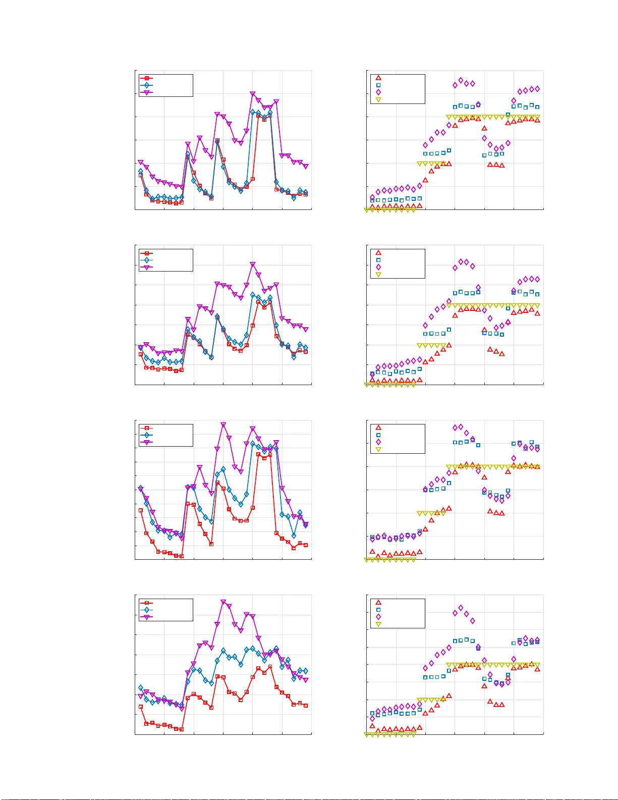
SUBMITTED FOR PUBLICA TION 1 Multi-T ar get T racking in Distrib uted Sensor Netw orks using P article PHD Filters Mark R. Leonard, Student Member , EURASIP , and Abdelhak M. Zoubir , Member , EURASIP , Abstract Multi-target tracking is an important problem in civilian and military applications. This paper in vestigates multi-target tracking in distrib uted sensor netw orks. Data association, which arises particularly i n multi-object scenarios, can be tackled by various solutions. W e consider sequential Monte Carlo implementations of the Probability Hypothesis Density (PHD) ﬁ lter based on random ﬁ nite sets. This approach circumven ts the data association issue by jointly estimating all targets in the region of interest. T o this end, we develo p the Diffusion Particle PHD F ilter (D-PPHDF) as well as a centralized version, call ed the Multi-Sensor Particle PHD Filt er (MS-PPHDF ). Their performance is ev aluated i n terms of the Optimal Subpattern Assignment (OSP A) metric, benchmark ed against a distributed extension of the Posterior Cram ´ er-Rao Lower Bound (P CRLB), and compared to the performance of an existing distributed PHD Particle F i lter . F urthermore, t he robustness of the proposed tracking algorithms against outliers and their performance with r espect to different amounts of clutter is in vestigated. Index T erms Multi-target tracking, distributed target t r acking, Particle F ilter , PHD F i lter , robustn ess, P osterior Cram ´ er-Rao Lower Bound I . I N T RO D U C T I O N T HE p r oblem of multi-target tracking (MTT) is beco ming inc r easingly impor tant in many military a nd ci vilian application s such as air an d grou nd trafﬁc control, harbor surveillance, maritime trafﬁc control, or video co m municatio n and surveillance [1]–[3]. Distributed sen so r networks offer a d esirable p latform for MTT ap plications due to th eir low cost an d ease o f deploym ent, their lac k o f a sing le poin t of failure , as well as their inhe rent redun dancy and fault-tolerance [ 4]. A compreh ensive overview of the state-o f-the-ar t o f distributed sing le-target tracking (ST T ) is given in [5 ]. Distributed versions of the Kalman Filter [ 5], [6 ] and its n onlinear, non-Ga ussian counterp art, the Particle Filter (PF) [7], have been well-studied . Howe ver , they cannot be applied directly to MTT as they do not acc ount for th e p roblem of data association. Althou gh there are method s such as the Jo in t Pro babilistic Data Association Filter (JPD AF) [8] or the Mu ltiple Hy pothesis T racker (MHT) [9] that add ress this problem in STT alg orithms, th e resource constra in ts in sensor networks might pose a challen ge on ﬁnding suitable distributed implementa tio ns [ 1 0]. The Pr o bability Hypoth esis De nsity (PHD) ﬁlter [11], [12], in co ntrast, resorts to the concept of rand om ﬁnite sets (RFSs) to circumven t the pro b lem of d ata association altogethe r . The authors are with the Signal Processing Group, Institute of T elec ommunications, T echnisc he Unive rsit ¨ at Darmstadt, Darmstadt 64283, Germany (e-mail: leonard @spg.tu-darmstadt.de, zoubir@spg.tu-darmsta dt.de) Manuscript submitted Novembe r 27, 2018 SUBMITTED FOR PUBLICA TION 2 P S f r a g r e p l a c e m e n t s T arget 1 T arget 2 T arget 3 y[m] x[m] 0 0 5 5 15 15 25 25 10 10 20 20 3 0 -10 -10 -20 -20 - 3 0 -5 -5 -15 -15 -25 -25 (a) P S f r a g r e p l a c e m e n t s T a r g e t 1 T a r g e t 2 T a r g e t 3 y[m] x[m] 0 0 5 5 15 15 25 25 10 10 20 20 3 0 -10 -10 -20 -20 - 3 0 -5 -5 -15 -15 -25 -25 (b) Fig. 1: (a) Distributed sensor ne twork with 1-coverage of the r egion o f interest and 3 exemplary target tra cks. (b) Exa mple of tracking 3 targets w ith the Diffusion Particle PHD Filter (D-PPHDF). The small c o lored dots represent the target location estimates o btained by the re sp ectiv e nod e with the same color . Th e light gray d ots show the collective measurem ents obtained by all nod es in the n etwork. In this work , we in vestigate distributed MTT in a sensor network with 1-coverage of the r egio n of interest (R OI), i.e. , th e sensor nodes have non- or barely overlapping ﬁelds of view (FO Vs) and are distributed such th a t max imum area coverage is attained [13]. An exemplary network lay out with these pr operties is depicted in Fig u re 1a). Autono mous distribution algorithm s for realizing su ch a to pology have been studied in o ur previous work [1 4]. The no des in the network commun icate with their neighbo rs in order to collabo ratively detect and track targets in the R OI. In add ition, all of the sen sors are equipp ed with a signal p rocessing u nit, allowing them to fo rm decisions without a fu sion ce n ter . That way , th e network can auton omou sly reac t to events such as the detection o f an in truder witho ut relying on a n etwork o perator . For the sake of simplicity , the n etwork is considere d to be static. Howe ver , the conside r ation of mo bile sensor n odes would enable reaction s such as target pursuit or escape. Since the FO V an d commun ication radius of each nod e are limited , a target is only seen by a subset of th e network, which changes as the target moves th r ough the R OI. Hence, at each time instant, there is an a ctive and an in active part of the network. The g oal, thus, is to detect and observe the target in a distributed and collabor ativ e fashion as it travels across the R OI, ra th er than re aching a network- w id e con sensus on its state a n d have the estimate av ailable at each no de. In the sequ el, we d ev elop a distributed Particle PHD ﬁlter called Dif fusion Particle PHD Filter (D-PPHDF), wh ich uses neighbo rhood commun ication to collabo r ativ ely e stimate and track a single-sensor PHD at each node in the active sub network. In add ition, we formulate the Multi-Senso r Particle PHD Filter (MS-PPHDF), a centralize d exten sion of the D-PPHDF. The perfor mance of both algorith m s is ev aluated in ter ms of the Optim al Su bpattern Assignm ent (OSP A) m etric [15], wh ich is calculated for th e joint set o f target state estimates o f th e active subnetwork. Fur thermor e , a d istributed version of the Posterior Cram ´ er-Rao Lower Boun d (PCRLB) [16]–[ 18]—again av erage d over the acti ve subnetwork—is introduced and u sed as a SUBMITTED FOR PUBLICA TION 3 benchm a rk. Moreover , we investi gate th e r o bustness of the prop osed trackin g algorithm s against outlier s an d examine th eir perfor mance under different amoun ts of clu tter . Other d istributed solu tions fo r MTT in a m u lti-sensor setup using the PHD ﬁlter have b een stud ied, e.g., in [ 19], [2 0], [21]. Contrary to ou r a p proach , they eith e r assume overlapping FO Vs or em ploy a pairwise comm unication schem e. The commo n idea, however , is to extend th e single-sen so r PHD ﬁlter to the m ulti-sensor case th rough comm unication between mu ltiple nodes, or nodes and a fusion center . A more rig orous app roach fo r MTT with multiple sensor s is to use a mu lti-sensor PHD ﬁlter [ 22], [23], wh ic h seeks to estimate and track a single mu lti-sensor PHD instead of m ultiple sing le - sensor PHDs. In this work, we compar e our meth ods to the appr oach in [2 0] (adap ted to our scen ario), wh ic h is also based on sing le-sensor PHDs. The co nsideration o f metho ds based on a multi-senso r PHD will b e the focu s of f uture work. The paper is o rganized as follo ws: Section 2 presents the co nsidered state-space model and recap itulates the theory of RFSs as well as the PHD an d th e PHD ﬁlter . The p roblem of distributed MTT is add ressed in Section 3. Here, we will ﬁrst detail our m odiﬁcation o f Adap tive T arget Birth (A TB) before form ulating the D-PPHDF an d in vestigate its computation al complexity and com m unication load. In Section 4, the MS-PPHDF is developed and analyzed in terms o f comp utational complexity and com m unication load . Section 5 is dedic a te d to simulations. First, the Distributed Posterior Cram ´ er-Rao Lower Bound (DPCRLB) is in troduce d . Then, we present the simulatio n setup and discu ss our results. Fin ally , a con clusion is given in Sec tion 6. I I . M O D E L S A N D T H E O RY A. State-Spa ce an d Measurement Mode l A linear state-sp ace model is co nsidered for e a c h target at time instant i ≥ 0 . The target state vector s tgt ( i ) = [ x tgt ( i ) , ˙ x tgt ( i )] ⊤ contains the target lo cation vector x tgt as well as th e velocity vector ˙ x tgt . For the sake of simplicity , we restrict ourselves to a 2D-environment. The target state evolves accor ding to the state eq uation [24]: s tgt ( i ) = F ( i ) s tgt ( i − 1) + G ( i ) n tgt ( i ) . (1) The matrices F and G as well as the vector n tgt will be explain ed shortly . No de k ob ta in s a measurem e n t z k of the target location as given b y the measu rement equation [ 2 4]: z k ( i ) = H k ( i ) s tgt ( i ) + ν tgt k ( i ) , k ∈ M (2) with M = { m ∈ { 1 , . . . , N } | k x m ( i ) − x tgt ( i ) k 2 ≤ R sen } d enoting th e set of all no des m that are locate d such that the Euclidean d istan ce k x m ( i ) − x tgt ( i ) k 2 between their location x m and th e target location x tgt is no t greater th an their sensing radius R sen . Note that N is the total num ber of no des in the network. Fur thermor e , n tgt ( i ) ∼ N ( 0 2 , 1 , Q ( i )) an d ν tgt k ( i ) ∼ N ( 0 2 , 1 , R k ( i )) den ote th e state and me asurement noise pro cesses, respectively , with the zero- mean vector 0 2 , 1 = [0 , 0] ⊤ . Both noise pro cesses are spatially and temp orally white, as well as unc orrelated with the in itial target state s tgt (0) an d e ach oth e r SUBMITTED FOR PUBLICA TION 4 for all i . For the sake o f simplicity , we choose a time - in variant measu r ement noise covariance matrix R k ( i ) = R k = σ 2 r I 2 , (3) where σ 2 r is the variance of each co mponen t of the measurem ent noise an d I n denotes th e identity matrix of size n . In target tracking, th e mod e l matrices ar e u sually chosen to be time- in variant and given by [24] F =    I 2 ∆ i I 2 0 2 , 2 I 2    , G =    ∆ i 2 2 I 2 ∆ i I 2    , Q = σ 2 q I 2 , (4) where 0 2 , 2 is the 2 × 2 zero matrix. Furtherm ore, ∆ i is the time step interval in second s with which the state-space model progr esses. In additio n , σ 2 q denotes the variance o f a state noise compo n ent. W e assume that the sensor n odes only obtain informa tio n on the location of a target. One commo n set of measur ements that is often f o und in ap p lications at sea is the combinatio n of distance and bearing measuremen ts from which an estimate of the target loca tio n can easily be calculated. Since we are no t interested in the exact nature of the measured locatio n info rmation but rath er in how this infor mation is processed by d ifferent tracking algo rithms, we f ormulate o u r mea su rement mo d el based o n the loca l target location estimates at ea ch node. This gives u s a gene r al mod el th a t is ap plicable to a wide variety of app lication irr espective of the exact measurem ent quantities. T hus, we obtain a g eneral measur ement matrix H k of the fo rm H k =  I 2 0 2 , 2  . (5) B. Random F inite Sets ( RFSs) A rand om ﬁnite set (RFS) is an u norder ed ﬁnite set that is rand om in the number of its elem e nts as well as in their values [25]–[27]. Th erefore, RFS s are a natural ch oice fo r r epresenting th e multi-target states and measuremen ts in MTT: the state and measure m ent vector s of a ll targets a r e collected in co rrespon ding RFSs [28], [2 9]. Gi ven the realization Ξ i − 1 of the RFS Ξ i − 1 at time instan t i − 1 , th e multi-target state of our tr acking pr o blem can be described b y the RFS Ξ i accordin g to Ξ i = S i (Ξ i − 1 ) ∪ B i , (6) where the survival set S i (Ξ i − 1 ) deno tes the RFS o f targets that alrea d y existed at time step i − 1 and have not exited the R OI, i.e., the region covered by th e sensor network, in the transition to time step i . In addition , the birth set B i is the RFS of new targets that spontan eously app ear at the bord er of the R OI at time instant i [1], [1 2], [29]. No te th a t th e statistical b ehavior of Ξ i can be de scr ibed by the condition al probab ility f i | i − 1 (Ξ i | Ξ i − 1 ) . The mu lti-target measuremen t mod el is given by the RFS Σ i as Σ i = Θ i (Ξ i ) ∪ C i (Ξ i ) , (7) where Θ i (Ξ i ) is the RFS of measuremen ts generated by Ξ i . In addition, the RFS C i (Ξ i ) represents clutter or false alarms. Giv en a re alization Σ i of Σ i , the statistical behavior of the RFS Σ i is descr ib ed by th e c o nditiona l prob ability f i (Σ i | Ξ i ) . SUBMITTED FOR PUBLICA TION 5 C. The Pr obab ility Hypoth esis Density (PHD) In analog y to the single-target case, the o p timal Bayesian ﬁlter for MT T recursively p ropag a tes the multi-target posterior f i | i (Ξ i | Σ 0: i ) over time, accord ing to f i | i (Ξ i | Σ 0: i ) = f i (Σ i | Ξ i ) f i | i − 1 (Ξ i | Σ 0: i − 1 ) R f i (Σ i | Ξ) f i | i − 1 (Ξ | Σ 0: i − 1 ) µ s ( d Ξ) (8) f i | i − 1 (Ξ i | Σ 0: i − 1 ) = Z f i | i − 1 (Ξ i | Ξ) f i − 1 | i − 1 (Ξ | Σ 0: i − 1 ) µ s ( d Ξ) , (9) where µ s is a dom inating measure as described in [29]. This appro ach requ ir es the ev aluation of multiple integrals, which makes it e ven more computationally ch allenging than its sin g le-target counterpart. A comm on solution is to ﬁnd a set o f statistics, e. g ., the moments of ﬁr st or second o r der, which yield a good a p proxim ation of the po sterior, and propag ate them instead [1]. The Proba b ility Hy pothesis Density (PHD) D i | i ( s ( i ) | Σ 0: i ) is an ind irect ﬁrst-o rder momen t of f i | i (Ξ i | Σ 0: i ) [30]. It is g iv en by the fo llowing integral [1 2], [31]: D i | i ( s ( i ) | Σ 0: i ) = X s tgt n ( i ) ∈ Ξ i Z δ ( s ( i ) − s tgt n ( i )) f i | i ( s ( i ) | Σ 0: i ) d s ( i ) , (10) where R f ( Y ) δ Y denotes a set integral. The PHD has the following two pro perties [30]: 1) The expected num ber of targets ˆ N tgt ( i ) at time step i is o btained by integrating the PHD accord in g to ˆ N tgt ( i ) = Z D i | i ( s ( i ) | Σ 0: i ) d s ( i ) . (11) This is in con trast to p r obability d e n sity fun ctions (PDFs), which always integrate to 1. 2) Estimates of the individual target states can b e foun d by searchin g for the j ˆ N tgt m highest p eaks of the PHD, where ⌊·⌉ denotes r oundin g to the nearest in teger . Because of th ese two prope r ties, the n umber of targets as well as their states ca n be estimated inde penden tly at each time step without any knowledge of their id e ntities. That way , the data association issue is av oide d . Howev er, this a lso m eans that PHD Filters canno t deliv er the continu ous track of a speciﬁc target. I f con tin uous track s are r equired, an add itional assoc ia tio n step has to be perf ormed. T wo possible a ssocia tio n algo rithms fo r track co ntinuity can b e foun d in [1 1]. D. The PHD F ilter The PHD Filter is an a p proach for rec u rsiv ely propa g ating the PHD D i | i ( s ( i ) | Σ 0: i ) at time step i given mea su rements up to time step i over time. I f the RFS Ξ is Poisson-distributed, th en its PHD is equal to its intensity fun ction and is, hence, a SUBMITTED FOR PUBLICA TION 6 sufﬁcient statistic [1 2]. In this c a se, th e PHD recursion is g iv en by the following p rediction an d upd ate equ ations [12]: D i | i − 1 ( s ( i ) | Σ 0: i − 1 ) = b i ( s ( i )) + Z p S ( s ( i − 1 )) f i | i − 1 ( s ( i ) | s ( i − 1 )) D i − 1 | i − 1 ( s ( i − 1 ) | Σ 0: i − 1 ) d s ( i − 1 ) (12) D i | i ( s ( i ) | Σ 0: i ) = " 1 − p D + X z ∈ Σ i p D f i ( z | s ( i )) λ F A c F A ( z ) + p D R f i ( z | s ( i )) D i | i − 1 ( s ( i ) | Σ 0: i − 1 ) d s ( i ) # D i | i − 1 ( s ( i ) | Σ 0: i − 1 ) (13) Note that b i ( s ( i )) is th e PHD of the bir th set B i of n ew targets app e a ring at tim e step i . In add itio n, p S ( s ( i − 1)) den otes the probab ility that a target survives the transition from time step i − 1 to i . The pr obability of survival depend s on the previous state s ( i − 1) because a target that is close to the bo rder o f the ROI and has a velocity vecto r poin ting away from it is unlikely to be p resent at time step i . Further more, f i | i − 1 ( s ( i ) | s ( i − 1)) an d f i ( z | s ( i )) d enote the transition pro bability and the likelihood, resp e c ti vely . T he pr obability o f detection p D is constant over tim e a n d the tr a cker’ s ﬁeld of view (FO V) since it is assumed th at a ll targets can be d etected if th e ROI is covered. The term λ F A c F A ( z ) repr esents Poisson-d istributed false-alarm s due to clu tter , where λ F A is the false alarm p arameter, wh ich is distributed accor ding to its spatial distribution c F A ( z ) . I I I . D I S T R I B U T E D M U LT I - T A R G E T T A R G E T T R A C K I N G In this section we introdu ce the Diffusion Particle PHD Filter (D-PPHDF), a distributed Particle Filter im plementatio n of the PHD Filter for per forming MTT in a sensor n etwork witho ut a fusion ce nter . Before diving into the alg o rithm, we brieﬂy revie w the concept of Ad aptive T arget Birth (A TB) a n d discu ss the mod iﬁcation we ap p lied in the D-PPHDF. A. Adaptive T ar get Birth (ATB) Standard formulatio ns of the PHD Filter consider the PHD b i ( s ( i )) of the birth set B i to be known a priori [32]. For typ ical tracking ap plications such as air surveillance, this is a reason a ble assumption since new targets shou ld app ear at the bo rder of the R OI g iv en continu o us observation. An alternative is to make the target bir th p rocess ada ptiv e an d mea su rement-d riv en as suggested in [32], [3 3]. T o this end, the PHD—an d con sequently the set of p articles and weights appr oximating it in a Particle Filter impleme ntation—is split into two densities co rrespond ing to persistent ob jects, w h ich have sur v iv ed the tran sition fro m time step i − 1 to i , and newborn objects, respectively . In [32], [33], the PHD o f newborn o bjects is appro ximated by randomly placing N P new par ticles around each target measuremen t, with N P denoting the numb er of particles per target. W e improve upon this app roach by only conside ring measuremen ts with no n oticeable impact o n any p ersistent particle weight, as th ese may indic a te th e appearance o f a n ew target. T h at way , the num b er of newborn par ticles is further reduced an d a p ossible overlap b e tween per sistent and newborn PHD is av oided. W ith the transition to time step i + 1 , the n ewborn p articles becom e p ersistent. Furth erore, we p erform the A TB step towards th e en d of each iteration of the a lg orithm and only c onsider the particles rep resenting the persistent PHD in the p rediction, weightin g, and r esampling steps. He n ce, the up date equation (13) d oes not have to be modiﬁed as in [3 2], [33]. While A TB de la y s the trac king algor ithm by one time step, it is much more efﬁcient as it only places new particles in regions in which a target is likely to b e found . In additio n , there is no need for an explicit in itialization step since the ﬁrst incoming target will tr igger the deployment o f a newborn p article clou d aro und its correspo nding m easurement. SUBMITTED FOR PUBLICA TION 7 B. The Diffusion P article PHD F ilter (D-P PHDF) The prop osed Diffusion Particle PHD Filter ( D- PPHDF) is an extension o f th e single-sen so r Particle PHD Filter (PPHDF) [11], [2 8], [34] f or the multi-sensor case. Furth ermore, it r elies on A TB for a more efﬁcient target detection. The commun ication scheme we employ to exchange m e a surements a n d estimates between node s is inspir ed by th e two-step com munication used in the context of Diffusion Ad a ptation [35]. Howev er, the algor ithm d oes not rely o n least-me a n-squares o r any other k ind of adaptive ﬁlter . First, e ach node k in th e activ e part of th e n etwork obtains an inter m ediate estimate o f the states of th e targets present, i.e., o f the PHD o f persistent targets—re p resented by th e set n s p k, pers ( i ) , w p k, pers ( i ) o N k, pers ( i ) p =1 of persistent par ticles with correspo n ding weights—based on neig hborh ood measur ements. In other words, every active nod e ru n s a separ a te PPHDF with access to mea surements fro m its neighbo rhood N k , d eﬁned as N k = { l ∈ { 1 , . . . , N }   k x l − x k k 2 ≤ R com } , k = 1 , . . . , N ., (14) where R com denotes the comm unication radius. Second , each active node combine s th e intermed ia te estimates from its neighbo rhood to a ﬁnal, collaborative estimate. T o this en d, the persistent particle sets of a ll neig hbors are merged in to a collective set n s p k, coll ( i ) , w p k, coll ( i ) o N k, coll ( i ) p =1 of per sistent neighb orhoo d particles and co rrespond ing weigh ts be f ore the clu stering step, with N k, coll ( i ) deno ting the numb er of collective persistent ne ighbor hood particles. In th e seq uel, we will lo ok at the individual steps of the D-PPHDF in mo re detail: • Mer ging : The sets n s p k, coll ( i − 1) , w p k, coll ( i − 1) o N k, coll ( i − 1) p =1 and n s p k, new ( i − 1) , w p k, new ( i − 1) o N k, new ( i − 1) p =1 consist of the collective persistent neighbo rhood p articles and newborn particles o f no de k , s p k, coll ( i − 1) and s p k, new ( i − 1) , respectively , at time step i − 1 with their respective weigh ts w p k, coll ( i − 1) an d w p k, new ( i − 1) . These sets are m erged to become the total set n s p k, tot ( i ) , w p k, tot ( i ) o N k, tot ( i ) p =1 of pa r ticles and weigh ts of n ode k at time step i . Here, N k, tot ( i ) is the to tal num b er of pa r ticles of nod e k at time step i , w h ich is given by N k, tot ( i ) = N k, coll ( i − 1) + N k, new ( i − 1) , (15) with N k, coll ( i − 1 ) an d N k, new ( i − 1 ) d e noting the respective nu mber of persistent neighb orhoo d and n ewborn particles at the previous time step. Note that since the sets o f particles and weigh ts re present PHDs, merging the sets co rrespon ds to summing the se PHDs. • Predicting: Eac h par ticle is propag ated thr ough the system model to beco me a persistent particle. Th e system mod e l is assumed to be the same fo r each target and given by Equ ation (1). Sinc e the p rocess noise is captured by the spre a d of the par ticle cloud , the r espective term can b e removed fro m the equ ation, yieldin g s p k, pers ( i ) = F s p k, tot ( i ) , p = 1 , . . . , N k, tot ( i ) . (16) The corre sponding we ights are multiplied with the pr obability of surviv al p S , which is assumed to be constant fo r th e SUBMITTED FOR PUBLICA TION 8 sake of simplicity 1 , ac cording to w p k, pers ( i | i − 1 ) = p S w p k, tot ( i ) , p = 1 , . . . , N pers ( i ) . (17) The pr ediction of particles a n d weigh ts co rrespond s to th e seco nd term in E quation (1 2). • Measuring & Br oadca sting (1): Th e sensor n o des obtain me a surements of the targets and forward them to their neig hbors. • W eighting: The p ersistent particle weigh ts of no de k a re updated by applying a weighting step c orrespon ding to Equation (13) iteratively for each ne ighbor . Using the pro duct oper a to r , th is weig h ting step can b e comp actly denoted as w p k, pers ( i ) = Y l ∈N k " 1 − p D + X z j ∈ Σ l i w p k,j, update ( i ) # w p k, pers ( i | i − 1 ) , (18) with w p k,j, update ( i ) = p D f i ( z j | x p ( i )) λ F A c F A ( z j ) + L ( z j ) , (19) where Σ l i is the set of measur e ments obtained b y no de l and L ( z j ) is calcu lated as L ( z j ) = N p k, pers ( i ) X q =1 p D f i ( z j | x q ( i )) w q k, pers ( i | i − 1 ) . (20) Note that f i ( z j | x p ( i )) is the likelihoo d and x p ( i ) is the location vecto r of particle p . Afterwards, each nod e k o btains the set Σ k i, cand of candidate m easurements, i.e., measurem ents that are not responsible for the hig hest weighting o f any pe r sistent particle, to be used in the A TB step later o n. Th e set Σ k i, cand is fo und accord ing to Σ k i, cand = Σ k i \ n z m p    m p = arg max j w p k,j, update ( i ) , p = 1 , ..., N k, pers ( i ) o . (21) • Resamp ling: Each node k calcu lates its own expected number o f targets ˆ N k, tgt ( i ) from its total persistent particle mass accordin g to ˆ N k, tgt ( i ) =     N k, tot ( i ) X p =1 w p k, pers ( i )     . (22) Consequently , th e num ber of p ersistent particles of nod e k is u pdated as N k, pers ( i ) = ˆ N k, tgt ( i ) N P . (23) Furthermo re, the set of p ersistent particles of n ode k has to b e resampled by drawing N k pers ( i ) particles with r e placement from it. Note that the pr obability of drawing particle p is given by w p k, pers ( i ) ˆ N k, tgt ( i ) since the weigh ts do not sum to unity . Then, 1 A constant probability of survi val p S is a reasonable assumption if the target s move relati vely slo wly with respect to the observa tion time and the size of the R OI. SUBMITTED FOR PUBLICA TION 9 the weigh ts are reset to equal values as w p k, pers ( i ) = ˆ N k, tgt ( i ) N k, pers ( i ) , p = 1 , . . . , N k, pers ( i ) . (24) • Br oadca sting (2): Every no d e k transmits its set of resampled pe r sistent particles and weights n s p k, pers ( i ) , w p k, pers ( i ) o N k, pers ( i ) p =1 to its neig h bors. • Clustering: Each node k f orms a collective set of persistent neig h borh o od par ticles s p k, coll ( i ) and cor r espondin g weights w p k, Nh ( i ) acc o rding to n s p k, coll ( i ) , w p k, coll ( i ) o N k, coll ( i ) p =1 = [ l ∈N k n s p l, pers ( i ) , w p l, pers ( i ) o N l, pers ( i ) p =1 , (25) with N k, coll ( i ) = X l ∈N k N l, pers ( i ) (26) denoting the n umber of collective persistent n eighbo rhood particles of node k . As in the merging step, this corr esponds to summing the corresp onding PHDs to ob tain an updated single-sensor PHD with a pro bability d istribution reﬂecting the informa tio n of the entire n eighbor hood of nod e k . Note that the PHDs might no t be ind ependen t if a target is d etected by more th an on e neigh bor . However , this is not a pro blem since merging the pa rticle sets simply results in th e respective target being repr esented by m ore par ticles. Hence, n ode k will be able to e stima te the cor r espondin g locatio n m ore accurately . The estimated target states are fo und b y clu stering the co llectiv e persistent particles. Sin ce the expected n umber of targets ˆ N l, tgt ( i ) , l ∈ N k might be d ifferent f or each n e ig hbor, we r esort to h ierar chical clu stering of the sing le-linkage typ e [36]. Here, the sum of the expected numb er of targets over th e n eighbo r hood c a n ser ve as an u pper b ound f or the numb er of clusters. Note, howev er, that if two targets are close to ea c h other, clustering algorith ms mig ht not be ab le to resolve both targets correctly . • Rou ghening : A roughen ing step is perf ormed to counter sample impoverishmen t [3 7]. T o this end, an inde p endent jitter s j ( i ) is added to every resam pled p article. Eac h component s j c ( i ) , c = 1 , . . . , d of the jitter with dim ensionality d is sampled f rom the Gaussian distribution N (0 , ( σ j c ( i )) 2 ) . Th e comp onent- w ise standard d eviation of the jitter is g i ven by σ j c ( i ) = K E c N k, coll ( i ) − 1 /d , (27) where E c is the interval length between the maximu m and m inimum samples of the respective com ponen t. T o a void ev aluating E c separately for each particle cluster, it is assign ed an em pirically found con stant value. 2 Note that d = 4 since the dime nsionality of the jitter vector s j ( i ) and the particle state vector s p ( i ) have to co incide. In additio n , K is a tuning con stant, which contr ols the sp read of the particle clo ud. • Ada ptive T a r get B irth: N P new par ticles are placed ran domly aro und each candidate measurement z j ∈ Σ k i, cand leading 2 Since the noise vari ances as well as the network topology are ﬁxed, the true value of E c will not change signiﬁcantl y over time and between clusters, so this is a val id simpliﬁcation. SUBMITTED FOR PUBLICA TION 10 to a total num ber of N k, new ( i ) = N P · | Σ k i, cand | n ewborn particles for no de k . E very newborn p article is associated with a weight tha t is chosen accord ing to w p k, new ( i ) = p B N p k, new ( i ) , p = 1 , . . . , N k, new ( i ) , ( 28) where p B is the p robability of birth. Dep ending on the app lication, p B can depen d o n time as well as on the lo cation of the respective p article. For simp licity , the probability tha t a new target enters the R OI is assumed to be eq ual for all locations in the birth region over time. Th e target birth pro cess correspo nds to th e ﬁrst term in Eq u ation (12). Figure 1 b) shows an example of trackin g three targets, which move along the d eterministic tracks d epicted in Figur e 1a), using the D-PPHDF. Note th at each small colored do t cor respond s to a target location estimate o btained b y the respective no de with the same colo r while the ligh t g rey dots rep resent the collective m easuremen ts from all no des. Fro m this illustration, the following pr operties of the D- PPHDF ar e appa r ent: First, the algorith m only de li vers sepa rate location estimates – represen ted by the small colored dots – for each time instan t ra th er than co ntinuou s tr a c ks, which – as m entioned b efore – is a co mmon proper ty o f PHD ﬁlters. Second , the network as a wh o le would be ab le to correctly tr ack all thr e e targets, while a sing le node only o btains the locally relevant sub tr acks of the targets in its vicinity . Thir d, the emp loyed two-step comm unication scheme is able to extend the vicinity of a no de far beyon d its own sensing radius of R sen = 6 m. This can, f or instance, be seen f r om the fact that the lime-g reen n ode lo cated at [ − 14 , − 2 3] is ab le to obtain lo cation estimates of target 2, which en ters th e ROI from the sou th. Finally , Fig u re 1 b) also illustrates the reso lution p roblem o f cluster in g. When targets 1 an d 2 , wh ich en ter the R OI fro m the north an d the south , respectively , cross paths, the no des in their vicinity see them as ju st one target. This leads to a n agg regation of target location estimates aroun d [9 , 0] . The pseu do-cod e of the D-PPHDF is given in T able I. C. Computation al Comp lexit y a nd Comm unication Lo ad In th is section we take a lo ok at the comp utational complexity and the comm unication load th e D- PPHDF imp oses on each node in the active subnetwork. The following steps are perform ed at e very time instant i but time dep endency is omitted for simplicity . Note that each o f the steps scales with the number of active nodes when considerin g th e comp utational co m plexity of the ne twork a s a whole. • Prediction : The pred iction step d escribed by Equatio ns (16) an d (1 7) is perfo rmed for each p article at ev ery active node. Hence, it scales with the nu mber of particles N k, tot and th e d imensionality d o f the par ticle vectors. In order to ob tain a tractable expr ession for th e comp utational complexity , we assume e ach no de to have the same nu mber of p a r ticles N tot . ⇒ O ( N tot d ) • W eighting : Ea c h par ticle is updated in the weigh ting step g iv en by Equ ations (18)-(21). The we ight u p date as well as the designation of can didate measuremen ts fo r A TB de p ends on the n eighbo rhood size |N k | of no de k and th e num ber of measuremen ts   Σ l   of each of its n eighbo rs l . For tractability reasons, we assume each node to have th e sam e n umber o f neighbo rs N nb and to o b tain the same numb er of m e a surements N meas . ⇒ O ( N tot N nb N meas ) SUBMITTED FOR PUBLICA TION 11 1: input: d, E c , K , n, N , N P , p B , p S , λ F A , c F A 2: initialize: n s p k, coll (0) , w p k, coll (0) o N k, coll (0) p =1 = n s p k, new (0) , w p k, new (0) o N k, new (0) p =1 = ∅ . 3: while i ≤ n do 4: for k = 1 , . . . , N do 5: Merge the sets of co llec tive per sistent an d newborn particles with co r respond ing weights: n s p k, tot ( i ) , w p k, tot ( i ) o N k, tot ( i ) p =1 = n s p k, coll ( i − 1) , w p k, coll ( i − 1) o N k, coll ( i − 1) p =1 ∪ n s p k, new ( i − 1) , w p k, new ( i − 1) o N k, new ( i − 1) p =1 . 6: for p = 1 , . . . , N k, tot ( i ) do 7: Predict the new state of each p article and upd ate the weight with the prob ability o f surviv al p S : s p k, pers ( i ) = F s p k, tot ( i ) w p k, pers ( i | i − 1) = p S w p k, tot ( i ) . 8: Update th e weig hts using neighb orho o d m easuremen ts: w p k, pers ( i ) = Y l ∈N k " 1 − p D + X z j ∈ Σ l i w p k,j, update ( i ) # w p k, pers ( i | i − 1 ) , w p k,j, update ( i ) = p D f i ( z j | x p ( i )) λ F A c F A ( z j ) + L ( z j ) , L ( z j ) = N k, pers ( i ) X q =1 p D f i ( z j | x q ( i )) w q k, pers ( i | i − 1 ) . 9: end for 10: Form the set o f cand idate measurem ents for A TB: Σ k i, cand = Σ k i \ n z m p    m p = arg max j w p k,j, update ( i ) , p = 1 , ..., N k, pers ( i ) , j = 1 , ...,   Σ l i   ∀ l ∈ N k o . 11: Calculate th e estimated num ber o f targets: ˆ N k, tgt ( i ) =     N k, tot ( i ) X p =1 w p k, pers ( i )     . 12: Resample ˆ N k, pers ( i ) = ˆ N k, tgt ( i ) N P particles and reset the we ig hts: w p k, pers ( i ) = ˆ N k, tgt ( i ) N k, pers ( i ) , p = 1 , . . . , N k, pers ( i ) . 13: Merge th e sets o f per sistent neighb orhoo d p articles a n d weigh ts: n s p k, coll ( i ) , w p k, coll ( i ) o N k, coll ( i ) p =1 = [ l ∈N k n s p l, pers ( i ) , w p l, pers ( i ) o N l, pers ( i ) p =1 . 14: Use single-link age clu ster in g to identify ˆ N tgt ( i ) clu sters an d ﬁnd the set of estimated ta rget states n ˆ s l k ( i ) o ˆ N tgt ( i ) l =1 by calcu lating th e centro ids. 15: Add an ind epende n t jitter to eac h particle using a c o mpon e nt-wise stand a rd deviation of: σ j c ( i ) = K E c N k, coll ( i ) − 1 /d . 16: Place N P new particles ra ndomly arou nd each candidate me asurement z j ∈ Σ k i, cand . Set the weights as: w p k, new ( i ) = p B N k, new ( i ) , p = 1 , . . . , N k, new ( i ) . 17: end for 18: i ← i + 1 19: end while 20: retur n T ABLE I: The D iffusion Particle PHD Filter . SUBMITTED FOR PUBLICA TION 12 • Resamp ling : Th e estima tion of th e n umber of targets and the r esampling step in Equ ations (22)-(24) are line ar in the number o f par ticles used for the calculation [38]. For the sake of simplicity , we assume each ac ti ve n ode to have the same estimate o f the numb e r o f targets N tgt . ⇒ O ( N tot + N active N tgt N P ) • Clustering : The comp lexity of sing le-linkage clustering is cubic in the number of particles, i.e., in the numb er of neighb ors N nb of each n ode, the estimated n umber of targets N tgt , the number of particles p e r target N P , and the d imensionality d of the pa r ticles [39]. ⇒ O (( N nb N tgt N P d ) 3 ) • Rou ghening : Roug hening (Eq u ation (27)) is perf ormed f o r every collective particle an d is linear in the d imensionality of the par ticles. ⇒ O ( N nb N tgt N P d ) • Ada ptive T ar get Birth : The bir th p rocess depend s on the number of particles per target N P as well as the nu mber of candidate mea surements N cand , which is assumed equal f or each active n o de to ensure tractibility . ⇒ O ( N P N cand ) As far as the com munication load is concern e d, the D-PPHDF require s the broadcasting of measurements, i.e., 2 scalars per measuremen t, over th e neighbo rhood in th e ﬁrst br oadcasting step. In the second step, th e sets of p articles and we ights, i.e. , 5 scalars per particle, a r e transmitted. Clearly , the commu nication load strong ly d e p ends on the nu mber o f nodes in the network, or more p recisely the nu mber o f active no des an d the size of their re sp ectiv e neighbo rhood . As an extension of the D- PPHDF, one could th ink of chan ging the second broadcasting step and transmit Gaussian Mixture M o del rep resentations—instead o f the actual particles an d weights—that will be resampled at th e receiver no de (see e . g., [40]). That way , commun ic a tion load could be red uced to transmitting only a few scalar s in the second broad casting step at the cost of estimation acc u racy and additional co mputation al comp lexity . Howe ver , a tho r ough treatmen t of th is extension is beyon d the scope of this work. I V . C E N T R A L I Z E D M U LT I - T A R G E T T R A C K I N G Having p resented the D-PPHDF as a distributed solutio n for MTT in a sensor network, we pro pose the centralized co unterpa rt to o ur appr oach in th e seq uel. A. The Mu lti-Sensor P article P HD Fil ter (MS-PPH DF) The pr oposed Mu lti- Sen sor Particle PHD Filter (MS-PPHDF) is a c e n tralized, multi-sensor PPHDF tha t relies on a fusion center with access to the measurem ents of all nodes in the network. It is b ased on the form ulation o f the single-senso r PPHDF in [11], [28], [34] but with an extende d measur ement set c omprising the measurements of the entire n etwork. Hen ce, on e might obtain more than one measure m ent per target—a change to the typ ic a l assumption in target tracking that e a ch target produ ces at mo st on e measuremen t [8]. T o acco unt for this c h ange, we add a pre-clu stering step b e fore the weighting step and normalize the weigh t update acco r dingly . A similar p artitioning of the measuremen t set is used in exten ded target track ing, where a sensor can receive mu ltiple target reﬂections due to th e target’ s p hysical extent [4 1], [42]. SUBMITTED FOR PUBLICA TION 13 In the fo llowing, we will lo o k at the individual steps of th e algor ithm in more detail: • Mer ging : The sets { s p pers ( i − 1) , w p pers ( i − 1) } N pers ( i − 1) p =1 and { s p new ( i − 1) , w p new ( i − 1) } N new ( i − 1) p =1 consist o f th e p ersistent an d newborn particles, s p pers ( i − 1) an d s p new ( i − 1) , r e sp ectiv ely , at time step i − 1 with th eir respec tive weights w p pers ( i − 1) and w p new ( i − 1 ) . The se sets are me rged to b ecome the total set { s p tot ( i ) , w p tot ( i ) } N tot ( i ) p =1 of particles and weights at time step i . Here, N tot ( i ) is the total n umber o f particles at time step i , wh ic h is given by N tot ( i ) = N pers ( i − 1) + N new ( i − 1) , (29) with N pers ( i − 1 ) a nd N new ( i − 1 ) deno ting the respective number of p ersistent and newborn particles at the previous tim e step. • Predicting: As in the D-PPHDF, ea ch par ticle is pro p agated thr ough the system model acco rding to s p pers ( i ) = F s p tot ( i ) , p = 1 , . . . , N pers ( i ) = N tot ( i ) (30) to beco me a persistent particle. T he cor respond ing weights are multiplied with the prob a bility of sur viv al p S as w p pers ( i | i − 1 ) = p S w p tot ( i ) , p = 1 , . . . , N pers ( i ) . (31) • Measuring : The senso r n odes obtain measurem ents of the targets. • Pre-Clustering: Since ther e migh t b e more than one mea su rement per target, the m easuremen ts of th e entire n e twork are pre-clustere d before the weigh tin g step and each me a su rement is assigned a label C ( z ) th at reﬂects the card in ality of its own clu ster . This can be do ne, fo r instance , using single - linkage clusterin g [3 6]. The clusterin g is based on the distance between m easurements, i.e., sp a tially clo se measu rements ar e assumed to stem from the same target. Hence, when two or mo re targets ar e too close to e a ch oth e r, car dinality erro rs may occur . • W eighting: All av ailable target me asurements, which compr ise the set Σ i , are used to update th e persistent particle weig hts accordin g to w p pers ( i ) = " 1 − p D + X z j ∈ Σ i w p j, update ( i ) # w p pers ( i | i − 1 ) , (32) with w p j, update ( i ) = p D f i ( z j | x p ( i )) ( λ F A c F A ( z j ) + L ( z j )) C ( z j ) , (33) and L ( z j ) = N pers ( i ) X q =1 p D f i ( z j | x q ( i )) w q pers ( i | i − 1 ) . (34) Note that—in contrast to the D-PPHDF—th e weightin g step is applied on ly onc e u sin g the entire set of measur ements. Therefo re—and since there might b e more than one measurem e nt per target—we have to ensure that the weight update terms w p j, update —and consequently the par ticle weights—still sum to the number of targets present. T his is done by SUBMITTED FOR PUBLICA TION 14 normalizin g Eq u ation (33) with C ( z j ) , i.e. , th e cardin ality of the clu ster to which the cur rent m e a surement z j belongs. Afterwards, we form the set Σ i, cand of candida te m easurements for the A TB step accord ing to Σ i, cand = Σ i \ n z m p    m p = arg max j w p j, update ( i ) , p = 1 , ..., N pers ( i ) o . (35) • Resamp ling: The expected num b er o f targets ˆ N tgt ( i ) is calculated from th e to tal p ersistent particle mass a s ˆ N tgt ( i ) =     N tot ( i ) X p =1 w p pers ( i )     . (36) Consequently , th e num ber of p ersistent particles is upda ted accordin g to N pers ( i ) = ˆ N tgt ( i ) N P . (37) Furthermo re, the set o f persistent par ticles is resampled by d rawing N pers ( i ) particles with probab ility w p pers ( i ) ˆ N tgt ( i ) . Then , the weights are reset to equal values as w p pers ( i ) = ˆ N tgt ( i ) N pers ( i ) , p = 1 , . . . , N pers ( i ) . (38) • Clustering: In con trast to the D- PPHDF, there is only one estimate o f the expe cted n umber of targets. Hence, we can use k -mean s clustering [43] to ﬁnd the estimated target states b y gro uping the resamp led particles into ˆ N tgt ( i ) clusters an d calculating the cen tr oid of each cluster . • Rou ghening : Rough e ning is per formed analog ously to th e D-PPHDF. • Ada ptive T ar get Birth: N P new particles are placed ran domly ar o und each can didate m easuremen t z j ∈ Σ i, cand yielding a to tal numb er of N new ( i ) = N P · | Σ i, cand | n ewborn particles. The co rrespon d ing weigh ts are chosen accordin g to w p new ( i ) = p B N new ( i ) , p = 1 , . . . , N new ( i ) , ( 39) where p B is the pr o bability of b irth. The pseu do-cod e of the MS-PPHDF is given in T able II. B. Computationa l Complexity a nd Communica tion Load In this section we ana ly ze the com putationa l complexity and th e co mmunic a tio n load of th e MS- PPHDF. Th e following steps ar e p e rformed at every time instant i but time depen dency is omitted for simplicity: • Prediction : The prediction step described by E quations (30) an d ( 31) is perform ed for each of the N tot particles and is linear in the dimensio n ality d . ⇒ O ( N tot d ) • Pre-Clustering : The p re-clusterin g step r elies on sin g le-linkag e clu stering. T he complexity is ther efore cub ic in the total number o f measu r ements N meas . [ 39] ⇒ O ( N 3 meas ) SUBMITTED FOR PUBLICA TION 15 1: input: d, E c , K , n, N , N P , p B , p S , λ F A , c F A 2: initialize: { s p coll (0) , w p coll (0) } N coll (0) p =1 = { s p new (0) , w p new (0) } N new (0) p =1 = ∅ . 3: while i ≤ n do 4: Merge the sets of pe r sistent and newborn pa rticles with corresp onding weights: { s p tot ( i ) , w p tot ( i ) } N tot ( i ) p =1 =  s p pers ( i − 1) , w p pers ( i − 1)  N pers ( i − 1) p =1 ∪ { s p new ( i − 1) , w p new ( i − 1) } N new ( i − 1) p =1 . 5: for p = 1 , . . . , N tot ( i ) do 6: Predict the new state of each p article and upd ate the weight with the prob ability o f surviv al p S : s p pers ( i ) = F s p tot ( i ) w p pers ( i | i − 1 ) = p S w p tot ( i ) . 7: Cluster the mea surements using single- lin kage clustering and assign e ach me a surement z a label C ( z ) reﬂecting the cardinality o f its cluster . 8: Update th e weig hts using the m e asurements of the entire n etwork: w p pers ( i ) = " 1 − p D + X z j ∈ Σ i w p j, update ( i ) # w p pers ( i | i − 1 ) w p j, update ( i ) = p D f i ( z j | x p ( i )) ( λ F A c F A ( z j ) + L ( z j )) C ( z j ) , L ( z j ) = N pers ( i ) X q =1 p D f i ( z j | x q ( i )) w q pers ( i | i − 1 ) . 9: end for 10: Form the set o f cand idate measurem ents for A TB: Σ i, cand = Σ i \ n z m p    m p = arg max j w p j, update ( i ) , p = 1 , ..., N pers ( i ) , j = 1 , ..., | Σ i | o . 11: Calculate th e estimated num ber of targets: ˆ N tgt ( i ) =     N tot ( i ) X p =1 w p pers ( i )     . 12: Resample ˆ N pers ( i ) = ˆ N tgt ( i ) N P particles and reset the we ig hts: w p pers ( i ) = ˆ N tgt ( i ) N pers ( i ) , p = 1 , . . . , N pers ( i ) . 13: Find the set of estimated target states n ˆ s l ( i ) o ˆ N tgt ( i ) l =1 by u sing k - means clustering and ca lcu lating the centr o id of each clu ster . 14: Add an ind epende n t jitter to ea c h particle using a co mpon e nt-wise stand ard deviation of: σ j c ( i ) = K E c N pers ( i ) − 1 /d . 15: Place N P new pa rticles ra ndomly arou nd each candidate me a surement z j ∈ Σ i, cand . Set the weights as: w p new ( i ) = p B N new ( i ) , p = 1 , . . . , N new ( i ) . 16: i ← i + 1 17: end while 18: retur n T ABLE II : The Multi-Sensor Particle PHD Filter . SUBMITTED FOR PUBLICA TION 16 • W eighting : Ea c h par ticle is updated in the weigh ting step g iv en by Equ ations (32)-(34). The we ight u p date as well as the designation o f cand idate measurem e n ts f or A TB depend s o n the nu m ber o f measuremen ts N meas = | Σ | . ⇒ O ( N tot N meas ) • Resamp ling : Th e estima tion of th e n umber of targets and the r esampling step in Equ ations (36)-(38) are line ar in the number o f par ticles used f or the calcu lation [38]. ⇒ O ( N tot + N tgt N P ) • Clustering : In contrast to the D-PPHDF we c a n use k -m eans clustering. The co mplexity of Lloyd’ s imp lementation is giv en by [44] ⇒ O (( N tgt N P ) dN tgt +1 log( N tgt N P )) . • Rou ghening : Roughen ing is lin ear in the dimension ality of the particles and th e ir n umber . ⇒ O ( N tgt N P d ) • Ada ptive T ar get Birth : The bir th p rocess depend s on the number of particles per target N P as well as the nu mber of candidate mea surements N cand . ⇒ O ( N P N cand ) In summ ary , the co mputation al comp lexity of the MS-PPHDF is largely co mparab le to th at of th e D-PPHDF. The only exception is the pre-custer in g step, wh ich scales cubicly with the total numb er of mea su rements an d adds additio nal c o mplexity to the algorithm. As a tr adeoff the commun ic a tion load of th e MS-PPHDF clearly is lower compared to the D-PPHDF because there is on ly the initial transm ission of measurements from the nod e s to the fusion center . Howe ver , considering a setup with r elativ ely small commun ication ra d ii, this initial com munication step requires a lot o f relayin g and leads to high trafﬁc density in th e v ic in ity of the fusion center . Furthe r more, this commun ication stru cture exhib its a single point of failure while a d istributed sensor n e twork is inhe rently redu ndant. V . S I M U L A T I O N S In this section , we ev aluate the p erform ance of the D-PPHDF as well as the MS-PPHDF for tr acking multiple targets in a sensor network with 1- coverage. T o this end, we consider Gaussian measurement noise of dif fere n t variance as well as ε -con taminated noise with different co n tamination r atios to investigate the robustness of the algor ithms. In a d dition, the perfor mance fo r different amo u nts o f clutter is analyzed . W e comp are the pro p osed alg o rithms to the altern ativ e distributed PPHDF fro m [2 0], which will b e referr ed to as Distributed Data Fusion Particle PHD Filter (DDF-PPHDF). Here, each node runs its own PPHDF using o n ly its own measu rements. I n a subseq u ent step, the p a rticles are distributed over the neigh borho od and r eweighted by fusing th eir correspo nding Ex ponen tial Mixtur e Densities. Furthermo re, we form u late the DPCRLB as a lower bo und for ev aluating the perfor mance of the three algorithm s in terms of the OSP A [1 5] metr ic. In our simulations, we com pute the OSP A metric with respect to the joint set of target state estimates of the en tire ac tive network. Th e latter is foun d by clustering th e target state estimates of all active nodes. Furthermor e, we consider the squared OSP A metric scaled by the num ber of targets, i.e. , N tgt ·  ¯ d ( c ) p  2 , as in [4 5]. That way , we can u se the DPCRLB, wh ich will be in troduce d in the following, as a ben chmark . SUBMITTED FOR PUBLICA TION 17 A. The Distributed P osterior Cram ´ er -Ra o Lower Boun d (DPCRLB) Rather than evaluating th e perfor m ance of the different M T T algor ithms based on a n error metric, it makes m ore sense to derive a minim um variance bound o n the estimation error, which enab les an absolute p erforma nce evaluation. For time-inv ariant statistical models, the most common ly used bound is the Cram ´ er-Rao Lower Boun d (CRLB), which is given by the in verse of Fisher’ s in f ormation matrix [4 6]. In [ 45] an d [47], th e CRLB is used in the co ntext of m ulti-sensor MTT of an u nknown number o f u nlabeled targets in order to ev aluate the perfo rmance, as well as prove the asym ptotic efﬁciency of the PHD a s the nu mber of nodes goes to inﬁn ity . Since we are more interested in the trackin g behavior of a ﬁxed network over tim e , we resort to the Posterio r Cram ´ er-Rao Lower Bound (PCRLB), which is an extension of th e CRLB f or the time-variant case [16]. This bou nd can b e calculated seq u entially with the help of a Riccati-like recu r sion der iv ed in [48]. Furth ermore, in [17] an d [49], the PCRLB is adapted fo r an MTT scenario in wh ich the tracker can ob tain more than o ne mea su rement per target. Let π m i , m = 1 , ..., M denote the p robability that any measuremen t is associated with ta rget m at time instan t i as deﬁned in [18]. W ith the correspo nding stocha stic p r ocess Π m i , the new stochastic proce ss o f association pro babilities an d target states to be estima te d bec o mes Φ i =  Π 1: M i , Ξ 1: M i  . Fisher’ s infor mation matrix J Φ i =    J Π i J Ξ i Π i J Π i Ξ i J Ξ i    can now be form ed as described in [49] and [1 7]. However , as the n umber o f targets varies over time, i.e., targets migh t en ter or exit the R OI, J Φ i has to b e expanded or shrun k in the inv erse matrix d omain as described in [5 0]. The PCRLB B i at time instant i can b e obtained as the trace of the inv erted submatr ix J Ξ i accordin g to [49] B i = trace  h J Ξ i − J Π i Ξ i J − 1 Π i J Ξ i Π i i − 1  . (40) Note that, in a d istributed MTT scenar io, B i correspo n ds to a lower boun d on the estimation e rror of a centra l pr ocessing unit with access to all measurements. Since we are intere sted in comp letely distributed MTT with in-ne twork processing, we extend the PCRLB to th e Distributed Posterior Cram ´ er-Rao Lower Bou nd ( DPCRLB). T o this end, each nod e k co mputes its own PCRLB B k i considerin g on ly the measur ements of its two-hop n eighbo r hood , which is given by N (2) k = [ l ∈N k N l , (41) i.e., the n e ighbor s of n ode k and their n eighbor s. Furthermo re, o nly the targets within the sensing range of N k are taken into account. Clear ly , o nly nod es with a neigh borho od in the v icinity o f at least one target will be a b le to calcu late a PCRLB. The DPCRLB B i, dist at time instan t i is then obtained b y averaging over these values accordin g to B i, dist = 1 |M| X k ∈M B k i , (42) where M is the set of all nod es that ar e ab le to comp ute a PCRLB. SUBMITTED FOR PUBLICA TION 18 V A R I A B L E V A L U E D E S C R I P T I O N ∆ i 1 s time step o f the track in g algorithm N 30 number o f nod es σ 2 r 0.1, 0.3 m 2 compon entwise power o f meas. noise σ 2 q 0.01 m 2 compon entwise power o f state no ise ε 0.1, 0.3 contamina tio n ratio R com 2 R sen commun ication r adius R sen 6 m sensing radius E c 6 empirical in terval length for jitter K 0.2 tuning constant for rou ghening N P 500 number o f par ticles per target p B 0.8 probab ility of bir th p D 0.95 probab ility of de te c tion p S 0.98 probab ility of surv iv al λ F A 0.1, 0.3 av erag e no. of false alarms / clutter c F A ( z ) 1 π R 2 sen PDF of false alarms / clutter (un iform) c 2 cut-off value ( OSP A) p 2 order of th e OSP A metr ic T ABLE II I: Simulatio n para m eters B. Simulation Se tup In the f o llowing simu lations, a static sensor network as depicted in Fig ure 1 a) is used to perf orm MTT. T h e network is centered aroun d the point of o rigin [0 , 0] ⊤ and distributed such that 1 -coverage of the R OI is gu aranteed . It covers a n area of approx imately 2500 m 2 . Clutter is assumed Poisson an d uniformly distributed over th e sensing ra nge of each no de w ith an av erag e rate of λ F A = 0 . 1 and 0 . 3 . Moreover , we con sider Gaussian measuremen t noise with variance σ 2 r = 0 . 1 and 0.3 as well as ε -contamin ation noise with a ten-times high er variance and a contamin ation rate o f ε = 0 . 1 and 0.3. For the sake o f simplicity , collisions b etween targets and sensor nod es a re n eglected. An overview of all simulation par ameters is giv en in T able I II. Since the p urpose of this work is to introdu ce the MS- PPHDF as well as the D-PPHDF, verif y their fu nctionality , and c o mpare them to alternative a pproach es, we consider a rath er simple scenario with a h igh prob ability of detec tio n and relativ ely low clutter levels. In our fu ture work, we will study mor e sop histicated scenarios to d e ﬁne possible breakd own points o f our algor ithms. W e use the MS-PPHDF, the D- PPHDF, as well as the DDF-PPHDF to track three targets for i = 0 , ..., 30 . The targets en te r the R OI a t time steps i = 0 , 9 , 1 4 from the no rth, south, and west, r espectively . A Mon te Carlo simulation with N MC = 100 0 runs is performed to evaluate the perfo rmance of the tracking algorith ms in terms of the Optimal Subpattern Assignment (OSP A) metric. Note that the target trajectories as shown in Figur e 1a) a r e deter ministic, as is often th e case in ta rget tr a cking simulations [ 50] in order to g uarantee th e c o mparab ility of th e d ifferent Monte Carlo runs regarding , for instance, the numb er of targets p resent. SUBMITTED FOR PUBLICA TION 19 3 4 6 7 8 9 P S f r a g r e p l a c e m e n t s MS-PPHDF D-PPHDF DDF-PPHDF DPCRLB t r u e n u m b e r N tgt ·  ¯ d (2) 2  2 and B i, dist Time steps i (seconds) 0 0 5 5 15 25 10 20 30 3 5 0 . 2 0 . 4 0 . 6 0 . 8 1 1 . 2 1 . 4 1 . 6 1 . 8 2 (a) Squared and scaled OSP A compared to DPCRLB, σ 2 r = 0 . 1 0.5 1.5 2.5 3 3.5 P S f r a g r e p l a c e m e n t s MS-PPHDF D-PPHDF DDF-PPHDF D P C R L B true number N t g t ·  ¯ d ( 2 ) 2  2 a n d B i , d i s t Time steps i (seconds) 0 0 5 15 25 10 20 30 3 5 0 . 2 0 . 4 0 . 6 0 . 8 1 1 . 2 1 . 4 1 . 6 1 . 8 2 N est (b) Estimated number of targets, σ 2 r = 0 . 1 3 4 6 7 8 9 P S f r a g r e p l a c e m e n t s MS-PPHDF D-PPHDF DDF-PPHDF DPCRLB t r u e n u m b e r N tgt ·  ¯ d (2) 2  2 and B i, dist Time steps i (seconds) 0 0 5 5 15 25 10 20 30 3 5 0 . 2 0 . 4 0 . 6 0 . 8 1 1 . 2 1 . 4 1 . 6 1 . 8 2 (c) Squared and scaled OSP A compared to DPCRLB, σ 2 r = 0 . 3 0.5 1.5 2.5 3 3.5 P S f r a g r e p l a c e m e n t s MS-PPHDF D-PPHDF DDF-PPHDF D P C R L B true number N t g t ·  ¯ d ( 2 ) 2  2 a n d B i , d i s t Time steps i (seconds) 0 0 5 15 25 10 20 30 3 5 0 . 2 0 . 4 0 . 6 0 . 8 1 1 . 2 1 . 4 1 . 6 1 . 8 2 N est (d) Estimated number of targets, σ 2 r = 0 . 3 Fig. 2: Sim ulation I : Results for Gaussian noise and clutter rate λ F A = 0 . 1 . Th e left part of the ﬁgure shows the squared an d scaled Optimal Subpattern Assignm ent (OSP A) metric fo r each algorithm compar e d to the Distributed Posterio r Cram ´ er-Rao Lower Bound (DPCRLB), while the r ight pa r t comp ares the estimated to the true num b er o f targets. C. Simulation I : Results In the ﬁrst simulation, we co mpare the per forman ce of the MS-PPHDF and the D- PPHDF to the altern ativ e DDF-PPHDF and the DPCRLB, which ser ves as a b enchmar k. Measureme n t n oise is zero -mean Gaussian with variance σ 2 r = 0 . 1 , 0 . 3 and the av erag e n umber of clutter is 0 . 1 . The simulation results are de p icted in Figur e 2. While the to p part con siders zero-m ean Gaussian measureme nt noise with a per-componen t variance o f σ 2 r = 0 . 1 , the bottom part shows the r esults for σ 2 r = 0 . 3 . In addition to evaluating the p erform ance of the MS-PPHDF, the D- PPHDF, and the DDF-PPHDF in terms of the squared and scale d OSP A metric over time and comparin g it to the DPCRLB as can be seen in the left part of th e ﬁgure, we also look at the estimated number of targets, which is d epicted in th e r ight colu mn. Since the OSP A me tr ic co ntains a pen alty for an erro neous estimate of the num ber of targets, this side-by-sid e co mparison facilitates th e interpr etation of the tracking re sults. Let us start by considerin g Fig u res 2a) and 2b), i.e ., the case of σ 2 r = 0 . 1 . First o f all, we o bserve that neith er track ing SUBMITTED FOR PUBLICA TION 20 0.5 1.5 2.5 P S f r a g r e p l a c e m e n t s MS-PPHDF D-PPHDF DDF-PPHDF DPCRLB t r u e n u m b e r N tgt ·  ¯ d (2) 2  2 and B i, dist Time steps i (s) 0 0 5 15 25 10 20 30 3 5 0 . 2 0 . 4 0 . 6 0 . 8 1 1 . 2 1 . 4 1 . 6 1 . 8 2 (a) Squared and scaled OSP A compared to DPCRLB, σ 2 r = 0 . 1 0.5 1.5 2.5 P S f r a g r e p l a c e m e n t s MS-PPHDF D-PPHDF DDF-PPHDF DPCRLB t r u e n u m b e r N tgt ·  ¯ d (2) 2  2 and B i, dist Time steps i (s) 0 0 5 15 25 10 20 30 3 5 0 . 2 0 . 4 0 . 6 0 . 8 1 1 . 2 1 . 4 1 . 6 1 . 8 2 (b) Squared and scaled O S P A compared to DPCRLB , σ 2 r = 0 . 3 Fig. 3: Sim ulation I: Results for Gaussian noise and clutter ra te λ F A = 0 . 3 (zoomed in). T he squared an d scaled O p timal Subpattern A ssign ment (OSP A) metrics of u sin g the Multi-Sen sor Particle PHD Filter (MS-PPHDF), the Diffusion Particle PHD Filter (D- PPHDF), an d the Distributed Da ta Fu sio n Particle PHD Filter (DDF-PPHDF), a r e compared to the Distributed Posterior Cram ´ er-Rao Lower Bound (DPCRLB). algorithm p rovides an OSP A value or an estimate o f the n umber o f targets f o r i = 0 . This is expected and due to A TB, which initializes new par ticle cloud s based o n the measuremen ts from the previous time step. Thu s, target birth is delayed by one time step and tr a cking can only be perfor med for i > 0 . Th e sam e effect can b e witn essed at i = 9 and i = 1 4 , respectively , which ma r k the time instants at wh ich targets 2 and 3 enter the ROI . Here, the OSP A curves of all trackers exhib it a sp ike, which is due to the fact that th e n ewborn particles are not yet considered in the tr acker a n d, h ence, the numb er of estimated targets is too low , as can be seen in Figure 2b). Another sud den rise o f all the OSP A curves can be ob served in the time inter val 20 ≤ i ≤ 2 4 with a valley at i = 22 . Lookin g at the estimated nu m ber o f targets, we can a ttribute this pheno menon to th e fact that only two o f the three targets are recog nized b y the trackin g algorithms. Since the target trajectories are de terministic, we know th at in the g iv en time interval targets 2 and 3 c r oss paths. Due to the inability of the clustering algorithm to separate strongly overlapping sets of measuremen ts, the two targets merge into on e as long as they are clo se to each other . When the two targets occupy almost exactly the same position, i.e . , at i = 22 , the OSP A me tr ic decre ases due to the decrea se in measurem ent variance. A s the targets drift apart, the variance and with it th e O SP A m etric incr eases up to the p oint wh ere the two targets can be reco gnized as separ ate again and the cor respond ing penalty is switched off. Lookin g at the overall picture in Figure 2a), which shows the case of σ 2 r = 0 . 1 , it is evident that the cen tralized MS-PPHDF and the distributed D- PPHDF a c h iev e approx imately the same per forman ce with OSP A values closely ap proach in g the DPCRLB when the number of targets stays constant. Furthermor e, b oth algorithms deliver very accurate estimates of th e n umber of targets, giv en they are sep arable by clusterin g, as can b e seen in Figure 2b). The DDF-PPHDF, howev er, c ontinuo usly exhibits a worse perfor mance than the D- PPHDF, both in terms o f the OSP A metric as well as the e stimated nu mber of targets. This is wher e the additiona l commun ication in the pr o posed D-PPHDF shows its strength in redu cing uncertain ty due to measuremen t noise and clutter . Apart from achieving worse tracking results, the DDF-PPHDF also has more d ifﬁculty in separating targets 1 a nd SUBMITTED FOR PUBLICA TION 21 2 when they cro ss path s, resulting in an ear lier rise and a later fall o f the OSP A metric, compa red to o u r app roach. In th e case o f σ 2 r = 0 . 3 , th e overall p erform a n ce of the different tracking algorith ms is very similar to the case of σ 2 r = 0 . 1 . In o rder to make a statement on how the different tracking algorithm s co mpare, let us neglect the penalty due to an e rroneo us estimate of the numbe r o f targets and take a look at Figures 3a) and 3b), which are zoomed -in versions of Figu res 2 a) a n d 2c), r espectiv ely . In Figu r es 3 a) and 3 b) the DPCRLB is given as a benchmark for tra c king perform ance. One can observe that its value is always smaller or equal to th e respective measurem ent v ariance . As stated before, th e centralized MS-PPHDF a n d the distributed D-PPHDF exhibit very similar perfo rmance and deliver better track ing results than the DDF-PPHDF . While the MS-PPHDF achieves lower OSP A values than the D - PPHDF when the n u mber of targets stay s constant, i.e., f or 3 ≤ i ≤ 8 and 24 ≤ i ≤ 30 , the D-PPHDF perf orms better directly af ter a new target a ppears, i.e., f or 1 ≤ i ≤ 2 , 10 ≤ i ≤ 13 , and 15 ≤ i ≤ 18 . Th is is likely due to the fact that the two-step co mmunica tio n sch eme employed in the D-PPHDF is able to reduce the imp act of measureme n t n oise and clutter faster than the centralized MS-PPHDF c a n . Lookin g at the case of σ 2 r = 0 . 3 in Figure 3 b), we observe that the hig her measurem ent noise affects th e perf o rmance of all algorithms, r esulting in higher OSP A curves. Wh ile the OSP A curves of the MS-PPHDF and the DDF-PPHDF are propo rtionally shifted upward by a p prox im ately the same value, i.e., they are equally impacted by the high er no ise level, the D-PPHDF seems to b e slightly more affected by the change . Howe ver it still outperfo rms the DDF-PPHDF at all time instants. All in all, the p roposed D-PPHDF yields better p e rforman ce than the existing DDF-PPHDF in estimating the number of targets and track ing them, ir r espective o f the amoun t of measur ement noise. In add ition, it is also a bit faster in d eliv ering correct state estimates of new targets than the centralized MS-PPHDF and p erforms on ly sligh tly worse o nce the number of targets stays co nstant. In our future work, we will look at ways to further improve the perf o rmance of the MS-PPHDF and the D-PPHDF in orde r to ap proach the DPCRLB even more closely . D. Simulation II: Results In the secon d simulation, we e valuate the performa n ce o f the MS-PPHDF , the D-PPHDF and the DDF- PPHDF under a higher clutter r ate of 0 . 3 . The remaining par ameters are ch osen as in the previous simulation . Th e simulatio n results are shown in Figure 4. The top part con sid e rs zero- mean Gaussian mea su rement no ise with a pe r-component variance of σ 2 r = 0 . 1 while the bottom par t shows the r esults fo r σ 2 r = 0 . 3 . While the h igher clu tter rate causes an in crease in the OSP A value of all algo r ithms, the MS- PPHDF is still ab le to corre c tly estimate the nu mber of targets (except for the c rossing p eriod 20 ≤ i ≤ 24 ) in both cases. When tak ing th e next lower integer of the estimate, the D-PPHDF also yields accep table r esults for σ 2 r = 0 . 1 . For σ 2 r = 0 . 3 the n umber of targets is overestimated by 1 fo r 1 ≤ i ≤ 15 , cau sing a stronger degradation of the scaled an d squa r ed OPSA value in this interval. Apparen tly , the DDF-PPHDF is no t able to co pe with a clu tter rate of 0 . 3 as the numb er o f targets is largely overestimated. Hence, n o accu r ate target tracking is possible. SUBMITTED FOR PUBLICA TION 22 4 6 8 12 14 16 18 P S f r a g r e p l a c e m e n t s MS-PPHDF D-PPHDF DDF-PPHDF D P C R L B t r u e n u m b e r N tgt ·  ¯ d (2) 2  2 and B i, dist Time steps i (seconds) 0 0 5 15 25 10 10 20 30 3 5 0 . 2 0 . 4 0 . 6 0 . 8 1 1 . 2 1 . 4 1 . 6 1 . 8 2 3 4 6 7 P S f r a g r e p l a c e m e n t s MS-PPHDF D-PPHDF DDF-PPHDF D P C R L B true number N t g t ·  ¯ d ( 2 ) 2  2 a n d B i , d i s t Time steps i (seconds) 0 5 5 15 25 10 20 30 3 5 0 . 2 0 . 4 0 . 6 0 . 8 1 1 . 2 1 . 4 1 . 6 1 . 8 2 N est 4 6 8 12 14 16 18 P S f r a g r e p l a c e m e n t s MS-PPHDF D-PPHDF DDF-PPHDF D P C R L B t r u e n u m b e r N t g t ·  ¯ d ( 2 ) 2  2 a n d B i , d i s t Time steps i (seconds) 0 0 5 15 25 10 10 20 30 3 5 0 . 2 0 . 4 0 . 6 0 . 8 1 1 . 2 1 . 4 1 . 6 1 . 8 2 N est 3 4 6 7 P S f r a g r e p l a c e m e n t s MS-PPHDF D-PPHDF DDF-PPHDF D P C R L B true number N t g t ·  ¯ d ( 2 ) 2  2 a n d B i , d i s t Time steps i (seconds) 0 5 5 15 25 10 20 30 3 5 0 . 2 0 . 4 0 . 6 0 . 8 1 1 . 2 1 . 4 1 . 6 1 . 8 2 N e s t N est Fig. 4: Simulatio n II: Results fo r Gaussian noise and clu tter rate λ F A = 0 . 3 . The left part of the ﬁgure shows the squared and scaled Optimal Subpattern Assignm ent (OSP A) metric fo r each algorithm compar e d to the Distributed Posterio r Cram ´ er-Rao Lower Bound (DPCRLB), while the r ight pa r t comp ares the estimated to the true num b er o f targets. E. Simulation II I: Results In the th ir d simulation , we ev aluate the robustness of the MS-PPHDF , the D-PPHDF and the DDF-PPHDF in the face of ε -contam inated noise an d different clutter rates. W e co nsider a per-compo nent variance of the measure ment noise of σ 2 r = 0 . 1 and 0 . 3 , an average nu mber of clutter of λ F A = 0 . 1 and 0 . 3 , as well as a contamin ation of 10% a n d 30% . The re m aining parameters ar e chosen as before . T he simula tio n results for clutter ra tes λ F A = 0 . 1 and 0 . 3 are given in Figu res ?? and 6, respectively . The top h alf o f each ﬁgure co nsiders σ 2 r = 0 . 1 wh ile the bottom half per ta in s to σ 2 r = 0 . 3 . Rows 1 and 3 dea l with a n o ise contam ination of 10 % , rows 2 a n d 4 show the results f o r 30 % . Let us loo k at the case of λ F A = 0 . 1 ﬁrst. W e ob serve that the c e n tralized MS-PPHDF is still th e best perfor ming algor ith m, being largely unaffected b y higher noise variance and o utliers. The D-PPHDF is a close second , b eing primarily affected by the higher clutter rate an d th e higher noise variance. It sh ows o nly a slight ad ditional perfo rmance degradation when in creasing the noise contamin ation to 3 0 % . Hen ce, it can b e said tha t bo th algorithm s are ro bust ag ainst o utliers and ca n h andle a f r action of at least 10 % in the given scenario. Th e MS-PPHDF can also cope with λ F A = 0 . 3 while the target position estimates o f the D-PPHDF m ight b e too imp r ecise in this case, depen ding on th e p roblem at han d. T he DDF-PPHDF, in contrast, is mo re se verely affected by outlier s. Both the OSP A value a nd the estimated n umber of targets incr e ase with the intr oduction of noise SUBMITTED FOR PUBLICA TION 23 contamina tio n. When the nu mber of targets rema ins co nstant and no target crossing takes place, i.e. fo r i < 9 an d i > 24 , the number o f targets is only slightly overestimated. Howev er, whe n targets two and th ree enter the scene, i.e. f or 10 ≤ i < 20 , the estimate is inaccu rate, which im poses a penalty on the scaled an d squared OPSA metric. Henc e, th e DDF- PPHDF is no t a r o bust alg orithm fo r the considered tr acking scenar io. In the case o f λ F A = 0 . 3 , the DDF-PPHDF, again, breaks down com pletely . The MS-PPHDF, howe ver , is still ab le to giv e accur a te re su lts with only sligh t d eviations from th e tru e num ber of targets and a small OSP A value. Un fortuna tely , the combinatio n of noise contamin ation and more clutter is too much for the D-PPHDF to han dle. It overestimates the nu mber of targets by o ne to two, cau sing the OSP A value to rise as well. In summ ary , th e pro posed MS-PPHDF and D- PPHDF are—to a ce r tain extent—robust against ou tliers of the ε -contamin ation kind. This pro p erty is d ue to the emp loyed two-way commu nication sch eme, which vets measuremen ts as well as intermediate target position estimates ag ainst the entire n etwork or the neig h borh o od of e a ch node. T he alternative D DF- PPHDF, h owe ver , breaks d own in the face of outliers. In [51]–[53], we successfully pr o posed to use rob ust es timator s to robustify seque n tial detectors for distributed sensor networks. W e app lied the same concep t to the distributed D - PPHDF. However , n o further perfor m ance impr ovement could be gained her e since the twofo ld neigh borh o od av erag ing alr e ady exhau sted the power of neigh borho od commun ication. V I . C O N C L U S I O N In this work, we d ev eloped a distributed as well as a centralized PPHDF for MTT in sensor networks. W e, furth e r more, came up with a distributed version o f the PCRLB that served as a ben chmark in the perfor m ance evaluation. Our simulation results showed tha t the d istributed D-PPHDF is faster in cor rectly tracking new targets th a n the centralized MS-PPHDF and perfor ms on ly slightly worse when the num ber of targets stays co nstant. In add ition, it delivers accur ate tracking re sults as long as the targets are far enou gh apart so that their co rrespond ing measure m ent clouds ar e sep a rable. Our appro ach ou tperfor ms the existing DDF-PPHDF at the cost of addition al co mmunic a tio n betwe en sensor nodes. Moreover, th e prop osed trackers are inheren tly robust a g ainst outlier s and th e centralize d MS-PPHDF is even ab le to ha n dle higher clutter rates. The existing DDF-PPHDF, in co ntrast, is neither r o bust n or ab le to cope with mo r e than 10 % clutter . A C K N OW L E D G M E N T The au thors would like to thank Dr . Paolo Braca fro m the N A TO Science & T echno logy Organization, Centre for Maritime Research and Exp erimentation in L a Sp e zia, Italy , for his valuable c omments. R E F E R E N C E S [1] S. Challa, R. Evans, M. Morelande, and D. Musicki, Fundamentals of object trac king . Ca mbridge Unive rsity Press, 2011. [2] S. Maresca, P . Braca, J. Horstmann, and R. Grasso, “Maritime surveill ance using multiple high-frequen cy surface-w ave radars, ” Geoscienc e and Remote Sensing , IEEE T ransactio ns on , vol. 52, no. 8, pp. 5056–5071, Aug 2014. [3] J. Rambach, M. F . Huber , M. R. Balthasar , and A. M. Zoubir , “Collabora ti ve multi-ca mera face recognit ion and tracking, ” in Proce edings of the 12th IEEE Internatio nal Confer ence on Advanced V ideo- and Signal-based Surveill ance (A VSS2015) , August 2015. SUBMITTED FOR PUBLICA TION 24 [4] R. Olfati-Sa ber , J . A. Fax, and R. M. Murray , “Consensus and cooperation in network ed multi-a gent systems, ” Proc eedings of the IEEE , vol. 95, no. 1, pp. 215–233, Jan 2007. [5] O. Hlinka, F . Hlaw atsch, and P . M. Djuric, “Distribu ted partic le ﬁlterin g in agent networks: A survey , classiﬁca tion, and comparison, ” IEEE Signal Pr ocessing Magazine , vol. 30, no. 1, pp. 61–81, 2013. [6] F . S. Catti vel li, C. G. Lopes, and A. H. Sayed, “Diffusi on strate gies for distrib uted Kalman ﬁltering: Formulati on and performance analy sis, ” Proc eedings of the 1st IAP R W orkshop on Cognit ive Information Pr ocessing (CIP) , pp. 36–41, 2008. [7] M. Arulampalam, S. Maske ll, N. Gordon, and T . Clapp, “ A tutoria l on partic le ﬁlters for online nonlinear/non- Gaussian Bayesian track ing, ” IEEE T ransac tions on Signal Proce ssing , vol. 50, no. 2, pp. 174–188, 2002. [8] Y . Bar-Shalo m, P . K. Wil lett, and X. Tian, T racki ng and Data Fusion: A Handbook of Algorithms . Storrs, CT: YBS Publishing, 2011. [9] D. Reid, “ An algorit hm for tracking multiple target s, ” IEE E Tr ansactions on Automatic Contr ol , vol . 24, no. 6, pp. 843–854, 1979. [10] S. Oh, L. Schenato, P . Chen, and S. Sastry , “Trac king and coordinatio n of multiple agents using sensor netw orks: System design, algorithms and expe riments, ” Procee dings of the IEE E , vol. 95, no. 1, pp. 234–254, 2007. [11] D. E. Clark, “Multipl e target trackin g with the probability hypothesis density ﬁlter , ” Ph.D. dissertation, Depart ment of Electrica l, Electronic and Computer Engineeri ng, Heriot-W att Univ ersity , UK, October 2006. [12] R. Mahler , “Multita rget Bayes ﬁltering via ﬁrst-order m ultita rget moments, ” IEEE T ransactio ns on Aerospa ce and Electr onic Systems , vol. 39, no. 4, pp. 1152–1178, 2003. [13] X. W ang, G. Xing, Y . Zhang, C. Lu, R. Pless, and C. Gill, “Integ rated cov erage and connecti vity conﬁguration in wireless sensor netwo rks, ” in Proce edings of the 1st international confere nce on Embedded network ed sensor systems . A CM, 2003, pp. 28–39. [14] M. R. Balthasar , S. Al-Sayed, S. Leier , and A. M. Zoubir , “Optimal area cov erage in autonomous sensor networks, ” in Proc eedings of the 2nd Internatio nal Confer ence and E xhibiti on on Underwate r Acoustics (UA2014) , J une 2014. [15] D. Schuhmacher , B.-T . V o, and B.-N. V o, “ A consistent metric for performance ev aluati on of multi-object ﬁlters, ” Signal Proc essing, IE EE T ransact ions on , vol. 56, no. 8, pp. 3447–3457, Aug 2008. [16] H. L. V an Tre es, Detection, estimation, and modulation theory . John Wile y & Sons, 2004. [17] C. Hue, J.-P . Le Cadre, and P . Perez, “Performance analysis of two sequential Monte Carlo methods and posterior Cramer-Rao bounds for multi-targ et tracki ng, ” in Pro ceedings of the F ifth Internation al Confer ence on Information Fusion , vol. 1, 2002, pp. 464–473. [18] ——, “Sequential Monte Carlo methods for multiple target tracking and data fusion, ” IE EE T ransaction s on Signal Proc essing , vol. 50, no. 2, pp. 309–325, 2002. [19] M. Uney , D. Clark, and S. Julier , “Distri buted fusion of PHD ﬁlters via exponenti al mixture densities, ” IE EE Journal of Selected T opics in Signal Pr ocessing , vol. 7, no. 3, pp. 521–531, June 2013. [20] M. Uney , S. Julier , D. Clark, and B. Ristic, “Monte Carlo realisation of a distrib uted multi-object fusion algorit hm, ” in Sensor Signal Proce ssing for Defenc e (SSPD 2010) , Sept 2010, pp. 1–5. [21] G. Battiste lli, L. Chisci, C. Fanta cci, A. Farina, and A. Graziano, “Consensus CPHD ﬁlter for distrib uted multitar get tracking, ” Selecte d T opics in Signal Pr ocessing, IEEE Journal of , vol. 7, no. 3, pp. 508–520, 2013. [22] R. Mahler , “The multisensor PHD ﬁlter: I. General soluti on via m ultita rget calc ulus, ” in Pr oc. SPIE Signal Proc essing, Sensor Fusion, and T arg et Recogn ition XV III , vol. 7336, May 2009. [23] ——, “ Approximat e multisensor CPHD and PHD ﬁlters, ” in Proce esings of the 13th Confer ence on Information Fusion (FUSION) , July 2010, pp. 1–8. [24] F . Gustafsson, F . Gunnarsson, N. Bergman, U. Forssell, J. Jansson, R. Karlsson, and P .-J. Nordlund, “Particl e ﬁlters for positioni ng, navigati on, and tracki ng, ” IEEE T ransactio ns on Signal Pr ocessing , vol. 50, no. 2, pp. 425–437, 2002. [25] B. T . V o, “Random ﬁnite sets in multi-obj ect ﬁltering, ” Ph.D. dissertatio n, Uni versity of W estern Australia, 2008. [26] R. P . Mahler , Statistic al multisour ce-mult itarg et information fusion . Arte ch House, Inc., 2007. [27] ——, Advances in statistical multisourc e-multitar ge t informati on fusion . Arte ch House, 2014. [28] B.-N. V o, S. Singh, and A. Doucet, “Sequentia l Monte Carlo implementation of the PHD ﬁlter for multi-targ et tracki ng, ” in Pro ceedings of the 6th Internati onal Confere nce on Information Fusion , 2003, pp. 792–799. [29] ——, “Sequenti al Monte Carlo methods for multitar get ﬁltering with random ﬁnite sets, ” IE EE T ransact ions on A er ospace and Electr onic Systems , vol. 41, no. 4, pp. 1224–1245, 2005. [30] R. Mahler , “Multitar get moments and their applicatio n to multitar get tracking, ” T echnica l Report, DTIC Document , 2001. SUBMITTED FOR PUBLICA TION 25 [31] ——, “’Statistics 102’ for multisource-multi target detecti on and tracking, ” IEEE Journal of Selecte d T opics in Signal P r ocessing , vol. 7, no. 3, pp. 376–389, 2013. [32] B. Ristic, D. Clark, B.-N. V o, and B.-T . V o, “ Adapti ve targe t birth intensit y for PHD and CPHD ﬁlters, ” IEE E T ransactions on Aer ospace and E lectr onic Systems , vol. 48, no. 2, pp. 1656–1668, April 2012. [33] B. Ristic, D. Clark, and B.-N. V o, “Improv ed SMC implementa tion of the PHD ﬁlter , ” in Proce esings of the 13th Confer ence on Information Fusion (FUSION) , July 2010, pp. 1–8. [34] S. Hong, L. W ang, Z.-G. S hi, and K. S. Chen, “Simpliﬁed particle PHD ﬁlter for m ultipl e-targe t tracking : Algorit hm and architect ure, ” Pro gress In Electr omagnetics Researc h , vol. 120, pp. 481–498, 2011. [35] A. H. Sayed, “Diffusio n adaptation over netwo rks, ” in E-Refere nce Signal Pr ocessing , R. Chella ppa and S. T heodoridis, E ds. Ne w Y ork: Elsev ier , 2013. [36] B. Everit t, S. Landau, M. Leese, and D. Stahl, Cluster Analysis . John Wile y & Sons, 2011. [37] N. J. Gordon, D. J. Salmond, and A. F . M. Smith, “Nove l approach to nonline ar/non-Gaussia n Bayesian state estimation, ” in IEE Proc eedings F – Radar and Signal Proce ssing , vol. 140, no. 2, 1993, pp. 107–113. [38] F . Gustafsson, “Parti cle ﬁlter theory and practic e with positioning applic ations, ” IEEE Aer ospace and Electr onic Systems Magazine , vol. 25, no. 7, pp. 53–82, 2010. [39] F . Murtagh, “ A survey of recent adv ances in hierarc hical clustering algorit hms, ” The Computer Jo urnal , vol. 26, no. 4, pp. 354–359, 1983. [40] B.-N. V o and W .-K. Ma, “The Gaussian mixture probability hypothesis density ﬁlter , ” IEEE T ransac tions on signal proce ssing , vol. 54, no. 11, pp. 4091–4104, 2006. [41] K. Granstrom and U. Orguner , “ A PHD ﬁlter for trackin g multiple exte nded targets using random matrice s, ” IEEE T ransaction s on Signal Proce ssing , vol. 60, no. 11, pp. 5657–5671, Nov 2012. [42] K. Granstrom, A. Natal e, P . Braca, G. L udeno, and F . Seraﬁno, “PHD exte nded targ et tracking using an incohe rent X-band radar: Preliminary real-worl d expe rimental results, ” in 17th International Confere nce on Information Fusion (F USION) , July 2014, pp. 1–8. [43] J. MacQueen et al. , “Some methods for classiﬁca tion and analysis of multi vari ate observat ions, ” in Proc eedings of the 5th Berkele y Symposium on Mathemat ical Statistics and Pr obability , vol. 1, no. 281-297. Califo rnia, USA, 1967, p. 14. [44] M. Inaba, N. Katoh, and H. Im ai, “ Applications of weighted voronoi diagrams and randomizat ion to vari ance-based k-clustering: (extend ed abstract), ” in Proc eedings of the 10th A nnual Symposium on Computational Geometry , ser . SCG ’94. Ne w Y ork, NY , USA: A CM, 1994, pp. 332–339. [Online]. A vail able: http://doi.ac m.org/10.1145/17 7424.178042 [45] P . Braca, S. Marano, V . Matta, and P . Wille tt, “ Asymptotic efﬁc iency of the PHD in multitar get/multise nsor estimation, ” IEEE J ournal of Selecte d T opics in Signal Proce ssing , vol. 7, no. 3, pp. 553–564, June 2013. [46] S. M. Kay , Fundamentals of statistical signal proce ssing: Estimation theory . Prentice -Hall, Inc., 1993. [47] P . Braca, S. Marano, V . Matta, and P . Wi llett, “Multit arget-mul tisensor ML and P H D : Some asymptotic s, ” in P r oceeding s of the 15th International Confer ence on Informatio n Fusion (FUSION) , 2012, pp. 2347–2353. [48] P . Ti chavsk y , C. Muravc hik, and A. Nehorai, “Posterior Cramer-Rao bounds for discrete-t ime nonline ar ﬁltering, ” IE EE T ransac tions on Signal Proc essing , vol. 46, no. 5, pp. 1386–1396, 1998. [49] C. Hue, J.-P . Le Cadre, and P . P ´ erez, “Performance analysi s of two sequential Monte Carlo methods and posterior Cram ´ er-Rao bounds for multi-ta rget tracki ng, ” IRISA, T ech. Rep., 2002. [50] A. Bessell, B. Ristic, A. Farina, X. W ang, and M. Arulampal am, “Error performance bounds for tracking a manoeuvring targ et, ” in Pro ceedings of the 6th Internatio nal Conferen ce of Information Fusion (FUSION) , vol. 2, 2003, pp. 903–910. [51] W . Hou, M. R. Leonard, and A. M. Z oubir , “Robu st distrib uted sequentia l detection via robust estimati on, ” Proc eedings of the 25th E ur opean Signal Pr ocessing Confere nce (EUSIPCO) , Aug 2017. [52] M. R. Leonard and A. M. Z oubir , “Rob ust sequential detection in distributed sensor network s, ” IEEE T ransacti ons on Signal Proce ssing , Feb 2018, submitted. [Online]. A v ailable : https:// arxi v .org/abs/ 1802.00263 [53] M. R. Leonard, M. Stief el, M. Fauß, and A . M. Zoubir , “Robust sequential testing of multiple hypotheses in distribute d sensor netw orks, ” in Pr oceedin gs of the 43rd IEE E Internat ional Confere nce on Accoustics, Speech and Signal Proce ssing (ICASSP) , April 2018. SUBMITTED FOR PUBLICA TION 26 σ 2 r = 0 . 1 ε = 0 . 1 3 4 6 P S f r a g r e p l a c e m e n t s MS-PPHDF D-PPHDF DDF-PPHDF D P C R L B t r u e n u m b e r N tgt ·  ¯ d (2) 2  2 and B i, dist Time steps i (seconds) 0 0 5 5 15 25 10 20 30 3 5 0 . 2 0 . 4 0 . 6 0 . 8 1 1 . 2 1 . 4 1 . 6 1 . 8 2 1.5 2.5 3 3.5 4 P S f r a g r e p l a c e m e n t s MS-PPHDF D-PPHDF DDF-PPHDF D P C R L B true number N t g t ·  ¯ d ( 2 ) 2  2 a n d B i , d i s t Time steps i (seconds) 0 5 15 25 10 20 30 3 5 0 . 2 0 . 4 0 . 6 0 . 8 1 1 . 2 1 . 4 1 . 6 1 . 8 2 N est σ 2 r = 0 . 1 ε = 0 . 3 3 4 6 7 P S f r a g r e p l a c e m e n t s MS-PPHDF D-PPHDF DDF-PPHDF D P C R L B t r u e n u m b e r N t g t ·  ¯ d ( 2 ) 2  2 a n d B i , d i s t Time steps i (seconds) 0 0 5 5 15 25 10 20 30 3 5 0 . 2 0 . 4 0 . 6 0 . 8 1 1 . 2 1 . 4 1 . 6 1 . 8 2 N e s t N tgt ·  ¯ d (2) 2  2 and B i, dist 1.5 2.5 3 3.5 4 4.5 P S f r a g r e p l a c e m e n t s MS-PPHDF D-PPHDF DDF-PPHDF D P C R L B true number N t g t ·  ¯ d ( 2 ) 2  2 a n d B i , d i s t Time steps i (seconds) 0 5 15 25 10 20 30 3 5 0 . 2 0 . 4 0 . 6 0 . 8 1 1 . 2 1 . 4 1 . 6 1 . 8 2 N e s t N t g t ·  ¯ d ( 2 ) 2  2 a n d B i , d i s t N est σ 2 r = 0 . 3 ε = 0 . 1 0.5 1.5 2.5 3 3.5 4 4.5 5.5 P S f r a g r e p l a c e m e n t s MS-PPHDF D-PPHDF DDF-PPHDF D P C R L B t r u e n u m b e r N t g t ·  ¯ d ( 2 ) 2  2 a n d B i , d i s t Time steps i (seconds) 0 5 5 15 25 10 20 30 3 5 0 . 2 0 . 4 0 . 6 0 . 8 1 1 . 2 1 . 4 1 . 6 1 . 8 2 N e s t N t g t ·  ¯ d ( 2 ) 2  2 a n d B i , d i s t N e s t N tgt ·  ¯ d (2) 2  2 and B i, dist 1.5 2.5 3 3.5 4 P S f r a g r e p l a c e m e n t s MS-PPHDF D-PPHDF DDF-PPHDF D P C R L B true number N t g t ·  ¯ d ( 2 ) 2  2 a n d B i , d i s t Time steps i (seconds) 0 5 15 25 10 20 30 3 5 0 . 2 0 . 4 0 . 6 0 . 8 1 1 . 2 1 . 4 1 . 6 1 . 8 2 N e s t N t g t ·  ¯ d ( 2 ) 2  2 a n d B i , d i s t N e s t N t g t ·  ¯ d ( 2 ) 2  2 a n d B i , d i s t N est σ 2 r = 0 . 3 ε = 0 . 3 3 4 6 7 8 P S f r a g r e p l a c e m e n t s MS-PPHDF D-PPHDF DDF-PPHDF D P C R L B t r u e n u m b e r N t g t ·  ¯ d ( 2 ) 2  2 a n d B i , d i s t Time steps i (seconds) 0 5 5 15 25 10 20 30 3 5 0 . 2 0 . 4 0 . 6 0 . 8 1 1 . 2 1 . 4 1 . 6 1 . 8 2 N e s t N t g t ·  ¯ d ( 2 ) 2  2 a n d B i , d i s t N e s t N t g t ·  ¯ d ( 2 ) 2  2 a n d B i , d i s t N e s t N tgt ·  ¯ d (2) 2  2 and B i, dist 1.5 2.5 3 3.5 4 4.5 P S f r a g r e p l a c e m e n t s MS-PPHDF D-PPHDF DDF-PPHDF D P C R L B true number N t g t ·  ¯ d ( 2 ) 2  2 a n d B i , d i s t Time steps i (seconds) 0 5 5 15 25 10 20 30 3 5 0 . 2 0 . 4 0 . 6 0 . 8 1 1 . 2 1 . 4 1 . 6 1 . 8 2 N e s t N t g t ·  ¯ d ( 2 ) 2  2 a n d B i , d i s t N e s t N t g t ·  ¯ d ( 2 ) 2  2 a n d B i , d i s t N e s t N t g t ·  ¯ d ( 2 ) 2  2 a n d B i , d i s t N est Fig. 5 : Simulation I II: Results fo r ε -contamin ated noise and clutter r ate λ F A = 0 . 1 . The two u pper r ows c o nsider σ 2 r = 0 . 1 , the lower o nes show the results fo r σ 2 r = 0 . 3 . Rows 1 and 3 conside r ε = 0 . 1 , r ows 2 and 4 show the results for ε = 0 . 3 . SUBMITTED FOR PUBLICA TION 27 σ 2 r = 0 . 1 ε = 0 . 1 P S f r a g r e p l a c e m e n t s MS-PPHDF D-PPHDF DDF-PPHDF D P C R L B t r u e n u m b e r N tgt ·  ¯ d (2) 2  2 and B i, dist Time steps i (seconds) 0 0 5 5 15 15 25 25 10 10 20 20 30 3 5 0 . 2 0 . 4 0 . 6 0 . 8 1 1 . 2 1 . 4 1 . 6 1 . 8 2 3 4 6 7 8 P S f r a g r e p l a c e m e n t s MS-PPHDF D-PPHDF DDF-PPHDF D P C R L B true number N t g t ·  ¯ d ( 2 ) 2  2 a n d B i , d i s t Time steps i (seconds) 0 5 5 15 25 10 20 30 3 5 0 . 2 0 . 4 0 . 6 0 . 8 1 1 . 2 1 . 4 1 . 6 1 . 8 2 N est σ 2 r = 0 . 1 ε = 0 . 3 P S f r a g r e p l a c e m e n t s MS-PPHDF D-PPHDF DDF-PPHDF D P C R L B t r u e n u m b e r N t g t ·  ¯ d ( 2 ) 2  2 a n d B i , d i s t Time steps i (seconds) 0 0 5 5 15 15 25 25 10 10 20 20 30 30 3 5 0 . 2 0 . 4 0 . 6 0 . 8 1 1 . 2 1 . 4 1 . 6 1 . 8 2 N e s t N tgt ·  ¯ d (2) 2  2 and B i, dist 3 4 6 7 8 9 P S f r a g r e p l a c e m e n t s MS-PPHDF D-PPHDF DDF-PPHDF D P C R L B true number N t g t ·  ¯ d ( 2 ) 2  2 a n d B i , d i s t Time steps i (seconds) 0 5 5 15 25 10 20 30 3 5 0 . 2 0 . 4 0 . 6 0 . 8 1 1 . 2 1 . 4 1 . 6 1 . 8 2 N e s t N t g t ·  ¯ d ( 2 ) 2  2 a n d B i , d i s t N est σ 2 r = 0 . 3 ε = 0 . 1 P S f r a g r e p l a c e m e n t s MS-PPHDF D-PPHDF DDF-PPHDF D P C R L B t r u e n u m b e r N t g t ·  ¯ d ( 2 ) 2  2 a n d B i , d i s t Time steps i (seconds) 0 0 5 5 15 15 25 25 10 10 20 20 30 30 3 5 0 . 2 0 . 4 0 . 6 0 . 8 1 1 . 2 1 . 4 1 . 6 1 . 8 2 N e s t N t g t ·  ¯ d ( 2 ) 2  2 a n d B i , d i s t N e s t N tgt ·  ¯ d (2) 2  2 and B i, dist 3 4 6 7 8 9 P S f r a g r e p l a c e m e n t s MS-PPHDF D-PPHDF DDF-PPHDF D P C R L B true number N t g t ·  ¯ d ( 2 ) 2  2 a n d B i , d i s t Time steps i (seconds) 0 5 5 15 25 10 20 30 3 5 0 . 2 0 . 4 0 . 6 0 . 8 1 1 . 2 1 . 4 1 . 6 1 . 8 2 N e s t N t g t ·  ¯ d ( 2 ) 2  2 a n d B i , d i s t N e s t N t g t ·  ¯ d ( 2 ) 2  2 a n d B i , d i s t N est σ 2 r = 0 . 3 ε = 0 . 3 P S f r a g r e p l a c e m e n t s MS-PPHDF D-PPHDF DDF-PPHDF D P C R L B t r u e n u m b e r N t g t ·  ¯ d ( 2 ) 2  2 a n d B i , d i s t Time steps i (seconds) 0 0 5 5 15 15 25 25 10 10 20 20 30 30 35 0 . 2 0 . 4 0 . 6 0 . 8 1 1 . 2 1 . 4 1 . 6 1 . 8 2 N e s t N t g t ·  ¯ d ( 2 ) 2  2 a n d B i , d i s t N e s t N t g t ·  ¯ d ( 2 ) 2  2 a n d B i , d i s t N e s t N tgt ·  ¯ d (2) 2  2 and B i, dist 3 4 6 7 8 9 11 P S f r a g r e p l a c e m e n t s MS-PPHDF D-PPHDF DDF-PPHDF D P C R L B true number N t g t ·  ¯ d ( 2 ) 2  2 a n d B i , d i s t Time steps i (seconds) 0 5 5 15 25 10 10 20 30 3 5 0 . 2 0 . 4 0 . 6 0 . 8 1 1 . 2 1 . 4 1 . 6 1 . 8 2 N e s t N t g t ·  ¯ d ( 2 ) 2  2 a n d B i , d i s t N e s t N t g t ·  ¯ d ( 2 ) 2  2 a n d B i , d i s t N e s t N t g t ·  ¯ d ( 2 ) 2  2 a n d B i , d i s t N est Fig. 6 : Simulation I II: Results fo r ε -contamin ated noise and clutter r ate λ F A = 0 . 3 . The two u pper r ows c o nsider σ 2 r = 0 . 1 , the lower o nes show the results fo r σ 2 r = 0 . 3 . Rows 1 and 3 conside r ε = 0 . 1 , r ows 2 and 4 show the results for ε = 0 . 3 .

Multi-Target Tracking in Distributed Sensor Networks using Particle PHD Filters

Original Paper

Comments & Academic Discussion

Leave a Comment

Original Paper

Related Papers

Comments & Academic Discussion

Leave a Comment