Wireless Localization for mmWave Networks in Urban Environments
Millimeter wave (mmWave) technology is expected to be a major component of 5G wireless networks. Ultra-wide bandwidths of mmWave signals and the possibility of utilizing large number of antennas at the transmitter and the receiver allow accurate iden…
Authors: Macey Ruble, Dr. Ismail Guvenc
1 W ireless Localization for mmW a v e Networks in Urban En vironments Macey Ruble and ˙ Ismail G ¨ uvenc ¸ Dept. Electrical and Computer Engineering, North Carolina State Uni versity , Raleigh, NC 27695 Email: { mcruble,iguvenc } @ncsu.edu Abstract Millimeter wa ve (mmW ave) technology is e xpected to be a major component of 5G wireless networks. Ultra- wide bandwidths of mmW a ve signals and the possibility of utilizing large number of antennas at the transmitter and the receiver allow accurate identification of multipath components in temporal and angular domains, making mmW ave systems advantageous for localization applications. In this paper , we analyze the performance of a two-step mmW ave localization approach that can utilize time-of-arriv al, angle-of-arriv al, and angle-of-departure from multiple nodes in an urban environment with both line-of-sight (LOS) and non-LOS (NLOS) links. Networks with/without radio-en vironmental mapping (REM) are considered, where a network with REM is able to localize nearby scatterers. Estimation of a UE location is challenging due to lar ge numbers of local optima in the likelihood function. T o address this problem, a gradient-assisted particle filter (GAPF) estimator is proposed to accurately estimate a user equipment (UE) location as well as the locations of nearby scatterers. Monte Carlo simulations show that the GAPF estimator performance matches the Cramer-Rao bound (CRB). The estimator is also used to create an REM. It is seen that significant localization gains can be achie ved by increasing beam directionality or by utilizing REM. Index T erms 5G, A OA, A OD, TO A, CRLB, localization, mmW ave, REM, particle filter I . I N T RO D U C T I O N The demand for wireless broadband communication has been gro wing rapidly , which has been the dri ving force for the emergence of 5G cellular networks. It has recently been shown in the literature that millimeter wav e (mmW a ve) technology is not only feasible for dynamic outdoor cellular networks, but can facilitate a thousand fold increase in data capacity [1]–[4]. The mmW ave cellular networks are expected to first be deployed in dense urban envir onments where the global positioning system (GPS) signal may typically be unav ailable and the demand for lar ge data rates is high. W ith coverage ranges that can extend to hundreds of meters, the network must be solely responsible for localization, while also simultaneously achieving high data rates in such scenarios [1]. Communication performance in 5G networks will be limited by the amount of time required to align the highly directional beams of the communicating nodes, particularly for exhaustiv e beam searches, which are costly to capacity [5]. A network that is able to localize node positions can significantly reduce the time spent on beam alignment and increase capacity [6]. Thus, it is important to characterize the performance of mmW ave network localization for urban scenarios. November 3, 2021 DRAFT 2 Mi c r o w a v e fr equ enci es : • Omn i dir ecti onal an t en nas • Man y sc a t t er er s • Unab l e t o se par a t e p a ths mmW a v e fr eq ue nci es : • Di r ecti onali ty l i mit s nu mbe r of p a ths • E ach r e flect i on has s tr ong a t t en ua ti on • L OS and sing l e b ounce pa th as su mp ti on • Str ong es t l i nk s se l ect ed f or l oc ali z a ti on A O D A O A T O A T O A , A OD , and A O A c an all be mode l ed as Ga us sian Fig. 1: Signal propagation in microwa ve and mmW ave frequencies. W ireless localization with strictly non-line-of-sight (NLOS) paths is achiev able for omni-directional antennas by exploiting the time-of-arriv al (TO A), angle-of-arriv al (A O A) and angle-of-departure (A OD) measurements [7]–[9]. While accurately measuring A O A and A OD is relativ ely dif ficult at lower frequencies due to the rich scattering and poor path separability , this is much easier to achieve in mmW a ve channels leading to improved localization performance [10]. The mmW ave frequencies also allo w the use of ultra-wide bandwidths larger than 1 GHz, which helps in providing precise TO A estimates. Fig. 1 highlights channel characteristics of mmW a ve frequencies that offer adv antages over traditional microw ave frequencies for localization. A. Literatur e Review on mmW ave Localization There have been recent studies in the literature that ev aluate mmW a ve localization performance in various scenarios. Localization with receiv ed signal strength (RSS), TO A, and A O A are analyzed in [11] (separately and jointly for different measurement parameters) for LOS and NLOS scenarios, showing promising results with TO A and A OA, and less reliable results with RSS. A log-normal path loss model is used to ev aluate RSS, time-difference- of-arriv al (TDOA), and A OA localization methods for LOS paths in [12]. A mobile’ s location and orientation are estimated jointly in [13], [14] for mmW a ve systems. It is shown in these papers that a single fixed equipment (FE) is sufficient to localize a user equipment (UE), but only LOS paths are considered. A direct localization approach for a user connected with multiple FEs is introduced in [15], but NLOS paths are treated as interference and LOS paths are still required. At lower frequencies NLOS paths are treated as interference. A major advantage of mmW av e frequencies is that very fe w paths hav e significant recei ved signal strength, which results in channel sparseness [16]. This property enables NLOS paths to no longer be considered as interference, but to instead be exploited as paths with additional November 3, 2021 DRAFT 3 information that can improve localization performance [17]. The work in [10] sho ws that it is possible to use LOS and NLOS paths to determine the orientation and position of a node communicating with a single transmitter at mmW ave frequencies under certain conditions. Specifically , it is shown that sufficient conditions for position and orientation estimation require at least one LOS path or three NLOS paths. The Cramer-Rao bound for localization and orientation is deri ved and a localization algorithm is proposed that exploits channel sparseness to estimate A OD/A O A/TO A, which is then used to estimate user position and orientation. The work in [18] extends the Cramer-Rao bound to three dimensions. B. Summary of the Pr oposed mmW ave Localization T echnique The algorithm proposed in [10] is only suited for single transmitter scenarios. Ho wever , there may be scenarios where a single transmitter is unable to establish enough paths to meet the suf ficient conditions for localization. In this work, we consider scenarios that are not necessarily limited to a single transmitter . Instead, an initial access or beam alignment stage is used to obtain rough A OD/A O A/TO A estimates for LOS and NLOS paths from one or multiple transmitters. Then, the user position is estimated using the A OD/A O A/TO A estimates. This step requires optimizing a non-con ve x cost function with man y local maxima. T o accomplish this we propose a gradient-assisted particle filter (GAPF) estimator . While separately estimating TO A, A OD, and A O A is sub-optimal, it significantly reduces computational effort and allows links from multiple transmitting FEs to be used for localization. It should be noted that the work in [10] studies methods to jointly estimate and refine A OD/A O A/TO A for LOS and NLOS paths from a single FE. This process can be used to obtain improved A OD/A O A/TO A estimates for one FE at a time in place of the proposed reduced complexity first step. Then, these estimates can be combined and used in the second step for improved localization accuracy ov er the proposed reduced complexity approach. The reduced complexity approach is only considered in this work because the minimal processing approach to estimating A OD/A O A/TO A greatly reduces computation time and still achiev es adequate localization accuracy . The proposed method is best suited for en vironments where man y nodes are connected, such as a 5G network with many FEs in an urban environment where a single FE may not be able to establish enough paths to meet the sufficient conditions for localization. Urban en vironments with many buildings and large structures contain scatterers that remain fixed in space. The three dimensional spatial characteristics of the urban environment can be captured by radio-en vironmental mapping (REM) and later exploited to estimate scatterer locations for NLOS paths to improve localization [19]. The knowledge provided by localization and REM can be used to relax initial access requirements and improve capacity for 5G communication systems [20]. In this work, we study REM-assisted localization, which assumes scatterer locations are estimated a priori and can be used to improve localization performance. C. Methods/Experiments and Contributions of This W ork T o our best knowledge, mmW a ve network localization that exploits LOS and NLOS paths from multiple FEs in an urban en vironment utilizing TO A/A OA/A OD with/without REM has not been studied in the literature. This paper analyzes the localization performance of 5G mmW a ve communication networks specifically considering urban November 3, 2021 DRAFT 4 canyon and urban corner environments where directional beams are captured at the UE in the downlink from one or multiple FEs. The contributions of this paper are summarized as follows: • A reduced complexity two-step localization scheme is introduced where in the first step the receiver obtains rough estimates of A OD/A O A/TO A for LOS and NLOS paths from initial access or beam alignment stages from multiple FEs [10], [21]. The A OD estimate is obtained from a transmitted reference signal where the transmitter embeds the center beam direction and the A OA/T O A are estimated non-jointly by the receiv er . The second step uses the A OD/A O A/TO A estimates to estimate the receiver and NLOS scatterer location coordinates. • A gradient-assisted particle filter (GAPF) estimator is proposed as a maximum likelihood (ML) estimator to estimate the UE position and scatterer coordinates over a non-con ve x space. It is shown to hav e performance that matches the Cramer-Rao bound (CRB) through Monte-Carlo simulations. • Localization performance is analyzed in urban canyon and urban corner scenarios where a UE is connected with one FE or two FEs. • The localization accuracy of REM-assisted and non-REM-assisted network performance is analyzed. The performance of a perfect REM system that has perfect kno wledge of a scatterer locations (with no localization error) for each observed path is used to bound realistic REM systems. • The scatterer locations that are extracted from the proposed localization approach are used to create an REM. The rest of this paper is organized as follo ws. Section II introduces the mmW ave localization model and studies how LOS and NLOS paths can be separated for localization purposes. Section III discusses estimation methods and introduces the GAPF estimator for localization. Section IV deriv es the CRB for mmW av e localization performance. Section V compares estimator performance to the CRB, analyzes mmW ave localization performance in urban canyon/corner en vironments with/without REM, and examines the trade-off between system complexity and localization accuracy . Subsequently , the proposed estimator is used to create an REM. Finally , Section VI provides concluding remarks. I I . M M W A V E L O C A L I Z A T I O N S Y S T E M M O D E L This section introduces the downlink system model in a mmW a ve network from multiple FE nodes to a single UE node, where the UE estimates its own position. Without loss of generality , our results can also be extended to network-based localization relying on uplink mmW ave signals from the UE. First, the 2D system model for mmW ave urban localization is introduced. Then, differentiating LOS from NLOS paths is studied. Additionally , ray tracing techniques are used to further study the ef fects of directional beams at mmW ave frequencies and justify that the results in the included 2D model are representative of a full 3D model. A. Localization Model While the position of a UE in a wireless network can be estimated directly , it is often more practical to implement a two-step positioning approach that first determines a set of parameters such as TO A, A OD, or A O A, which are then used to estimate the position [22]. November 3, 2021 DRAFT 5 Scattere r: UE: FE : UE: NLOS LOS FE : (a) (b) Fig. 2: mmW a ve localization model for (a) NLOS and (b) LOS scenarios. The considered scenario utilizes the periodic beam training stage or initial access for mmW a ve network commu- nications to collect A O A/A OD/T OA for a variety of paths [6], [23]. The beam training stage searches ov er possible beams at the FE and UE where each directional beam points in a dif ferent direction. The beams with the strongest signals are then used to estimate A O A/A OD/TO A for the paths associated with those beams. A propagation channel is known to be sparse at mmW ave frequencies [16], [23], for which one major reason is the use of highly directional beams enabled at mmW ave frequencies with many antenna elements. Hence, each beam will typically contain a LOS path or a strong single bounce NLOS path [16], [24] along with multiple bounce NLOS paths that will hav e large attenuation and much lo wer signal strength [23]. Since only the strongest beams for each UE/FE pair are selected, multiple bounce paths are relatively unlikely , which allows the model to be simplified to LOS paths and single bounce NLOS paths [23]. Assuming a synchronized network, ultra-wide bandwidths of mmW a ve frequencies provide precise TO A estimates [25]. Measuring A O A and A OD is not feasible at lower frequencies because of large numbers of scattered paths. Howe ver , the arrays with large numbers of antenna elements at mmW ave frequencies easily fit on chip enabling highly directional beams. Arrays at the UE provide precise A OA measurements, where it is assumed the orientation of the UE is known so that the A O A relati ve to the ov erall coordinate system is determined from the A OA relativ e to the UE array . An A OD measurement is obtained from the FE, which transmits the beam’ s quantized A OD relativ e to the ov erall coordinate system. This is easily calculated from the A OD of the FE relati ve to the antenna array under the assumption that the FE orientation is known. Additionally , the FE is assumed to broadcast its position coordinates. These low complexity methods of obtaining A OA/A OD/TO A make mmW ave an ideally suited technology for localization. From the beam training stage, we assume that the A O A/A OD/TO A are measured for paths corresponding with beams from N FE FEs. Then, each path is identified as LOS or NLOS, which is discussed in II-C. It is assumed there are N L ≤ N FE LOS paths and N N NLOS paths, which are used to estimate the location of a UE at position p = [ p x p y ] T . (1) November 3, 2021 DRAFT 6 Fig. 2 shows a NLOS and a LOS path along with each path’ s associated parameters, which are explained in the following paragraphs. Let the vector q ∈ R 2 × N FE be the 2-dimensional coordinate vector for N FE transmitting FEs and q ( k j ) = [ q x ( k j ) q y ( k j )] T (2) be the location of FE k j that transmits path j . The vector s ∈ R 2 × N N is the 2-dimensional coordinate vector for the locations of all the scatterers of the NLOS paths, and s ( i j ) = [ s x ( i j ) s y ( i j )] T (3) is the location of scatterer i j that reflects path j . Let α ( θ ) ∈ R ( N L + N N ) × 1 contain the A O A for all LOS and NLOS paths, β ( θ ) ∈ R ( N L + N N ) × 1 contain the A OD for all LOS and NLOS paths, and d ( θ ) ∈ R ( N L + N N ) × 1 contain the total travelled path distance (which TO A will measure) for all LOS and NLOS paths. A NLOS path j transmitted from FE k j and reflected from scatterer i j will hav e A O A α j,k j ,i j , A OD β j,k j ,i j , and distance d j,k j ,i j . A LOS path j transmitted from FE k j will hav e A O A α j,k j , 0 , A OD β j,k j , 0 , and distance d j,k j , 0 where the index 0 signifies a LOS path. For consistency , let the first N L elements of α ( θ ) , β ( θ ) , and d ( θ ) correspond to LOS paths so that these elements hav e indices j = 1 , ..., N L ; k j = 1 , ..., N L ; and i j = 0 . The remaining N N elements are the remaining NLOS paths with indices j = N L + 1 , ..., N L + N N ; k j corresponds to the FE locations from which NLOS path j originated; and i j = 1 , ..., N N corresponds to the scatterer location from which path j reflects. Then, similar to [8], the measured/observed parameters for LOS paths to be used for localization can be written as α j,k j , 0 ( θ ) = atan2 q x ( k j ) − p x q y ( k j ) − p y ! , (4) β j,k j , 0 ( θ ) = atan2 p x − q x ( k j ) p y − q y ( k j ) ! , (5) d j,k j , 0 ( θ ) = q ( p x − q x ( k j )) 2 + ( p y − q y ( k j )) 2 . (6) On the other hand, NLOS paths hav e the parameters α j,k j ,i j ( θ ) = atan2 s x ( i j ) − p x s y ( i j ) − p y ! , (7) β j,k j ,i j ( θ ) = atan2 s x ( i j ) − q x ( k j ) s y ( i j ) − q y ( k j ) ! , (8) d j,k j ,i j ( θ ) = q ( s x ( i j ) − p x ) 2 + ( s y ( i j ) − p y ) 2 + q ( s x ( i j ) − q x ( k j )) 2 + ( s y ( i j ) − q y ( k j )) 2 , (9) November 3, 2021 DRAFT 7 where atan2 ( · ) is the four quadrant in verse tangent: atan 2 y x = atan y x if x ≥ 0 , atan y x + π if x < 0 and y ≥ 0 , atan y x − π if x < 0 and y < 0 , π 2 if x = 0 and y > 0 , − π 2 if x = 0 and y < 0 , undefined if x = 0 and y = 0 , (10) and atan ( · ) is the ordinary arctangent function. Our goal is to estimate p = [ p x p y ] T from noisy measurements of the parameters in (4)–(9) from multiple links with one or more FEs. The noise of the A OA/A OD/TO A path parameters is assumed to be zero-mean Gaussian throughout this paper and the estimation algorithm is designed under the Gaussian noise assumption. Though, the Gaussian distribution is just one possibility for parameter noise distributions. The proposed algorithms can still be used if the parameters have non-Gaussian noise distributions, but with degraded performance. The localization estimator is optimal under the Gaussian noise scenario, but scenarios with non-Gaussian distributions are still expected to hav e reasonable performance [26]. Nonetheless, the Gaussian assumption is reasonable for A O A/A OD/TO A at mmW ave frequencies as supported by [27]–[29], where [29] uses a measurement campaign to show that Gaussian noise is a good fit for A OD and A O A at mmW a ve frequencies in urban environments. TO A estimation can be used to determine the total distance in (6) and (9) traveled by a path for LOS and NLOS links, respectiv ely . The measured distance for a path is d 0 j,k j ,i j = d j,k j ,i j ( θ ) + n ( d ) j,k j ,i j , (11) with n ( d ) j,k j ,i j ∼ N (0 , σ 2 d l ) where l = L for LOS and l = N for NLOS paths. The center direction of the transmitted beam can be transmitted by the FE and used as an A OD estimate. The measured A OD is β 0 j,k j ,i j = β j,k j ,i j ( θ ) + n ( β ) j,k j ,i j , (12) with n ( β ) j,k j ,i j ∼ N (0 , σ 2 β l ) where l = L for LOS and l = N for NLOS paths. The A O A can be measured by a receiv er array so that the measured A O A is α 0 j,k j ,i j = α j,k j ,i j ( θ ) + n ( α ) j,k j ,i j , (13) with n ( α ) j,k j ,i j ∼ N (0 , σ 2 α l ) where l = L for LOS and l = N for NLOS paths. W ithout loss of generality , the v ariance of the parameters hav e been assumed to only depend on whether the path is LOS or NLOS. The parameters for the paths in (4)-(9) depend on the unknown position of the UE p and the unknown scattering locations s , which are nuisance parameters. The vector of unknown parameters that must be estimated is θ = [ p T s T ] T ∈ Θ , (14) November 3, 2021 DRAFT 8 where Θ ∈ R 2+2 N N is the unkno wn parameter space. W e also consider networks that hav e REM capabilities. REM provides information about the en vironment such as building locations and path link information, which can be used to determine scatterer locations and improv e localization performance. The best case scenario is when the REM can provide suf ficient information so that the scatterer locations are kno wn perfectly . Then, the estimator no longer has to estimate the scatterer locations for each NLOS path and only the UE position p needs to be estimated. Therefore, the performance of REM aided localization is bounded by the case where scatterer locations are kno wn and constant so that the UE position coordinates are the only parameters that need to be estimated and the unknown parameter vector becomes: θ = [ p ] ∈ Θ , (15) where Θ ∈ R 2 . With or without REM, the mmW av e parameter measurements in (4)-(9) can be characterized using a nonlinear Gaussian model, which fits the general form: z = h ( θ ) + w , (16) where the nonlinear function h : R N → R M and observations z are given by: h ( θ ) = [ α ( θ ) T β ( θ ) T d T ( θ )] T and z = [ ( α 0 ) T ( β 0 ) T ( d 0 ) T ] T . The measurement noise w ∼ N (0 , R ) is additi ve Gaussian noise from n ( d ) j,k j ,i j , n ( β ) j,k j ,i j , and n ( α ) j,k j ,i j with measure- ment cov ariance matrix, R = diag ( σ 2 α L ) 1 × N L , ( σ 2 α N ) 1 × N N , ( σ 2 β L ) 1 × N L , ( σ 2 β N ) 1 × N N , ( σ 2 d L ) 1 × N L , ( σ 2 d N ) 1 × N N . (17) Localization then requires estimating the UE position p from the measurements z . σ α L ( ◦ ) σ β L ( ◦ ) σ d L ( m ) σ α N ( ◦ ) σ β N ( ◦ ) σ d N ( m ) 28 GHz 10 . 5 8 . 5 0 . 75 10 . 1 9 . 0 0 . 75 73 GHz 8 . 5 5 . 5 0 . 75 6 . 0 7 . 0 0 . 75 T ABLE I: Standard deviation of the observation parameters that are used in the simulations. B. Statistics of AO A, A OD, and TO A The authors in [29] use measurements and simulations in urban environments to characterize the statistics of A O A, A OD, and TO A (needed for (17)) for a system with 2.5 ns multipath resolution and 800 MHz bandwidth, at center frequencies 28 GHz and 73 GHz. Horn antennas are used with 10 . 9 ◦ / 8 . 9 ◦ azimuthal/elev ation 3 dB beamwidths at 28 GHz and 7 ◦ / 7 ◦ azimuthal/elev ation 3 dB beamwidths at 73 GHz. It has been shown that the parameters given closely capture the statistics of measurements in urban en vironments at these frequencies. W e use these parameters for each receiv er in simulations, which are summarized in T able I. Using the model from [29] provides an accurate representation of an urban en vironment so that ray tracing is not necessary , which greatly simplifies simulations. It should be noted that the source of noise from the experimental campaign in [29], which November 3, 2021 DRAFT 9 (a) (b) (c) Fig. 3: (a) Geometry and ray tracing paths for W ireless Insite simulation in an urban en vironment. Paths are colored based on RSS where the strongest RSS path is red and the weakest RSS paths is green. (b) T OA of simulation with 80 ◦ 3 dB beamwidth. (c) TO A of simulation with 28 ◦ 3 dB beamwidth. leads to the variances in T able I is from multipath in the same timing bin and the inability to separate them. Antennas with more directionality will reduce the number of multipaths and reduce the noise v ariances from T able I and improve localization accurac y . The included A OD and A O A noise variances in T able I that are extracted from mmW ave measurements in [29] are assumed to capture the effects such as NLOS reflection power loss, beamwidth, and interfering multipath components. It should also be noted that these parameters assume the same receiv e SINR for both central frequencies of 28 GHz and 73 GHz as there are no interfering transmitters using the same bands; in other words, impact of central frequency is limited to the statistics reported on T able I, and interfering path behavior at these two dif ferent mmW a ve bands are not explicitly taken into account. On the other hand, mmW ave frequencies hav e little interference due to highly directional communications and highly attenuated reflections [1]. C. Differ entiating LOS and NLOS P aths A challenging aspect for mmW a ve localization will be LOS/NLOS path identification and path separation, which is needed for generating the vector of unknown parameters in (14) (includes one unkno wn scatterer location for each NLOS path, and no scatterer for a LOS path), the cov ariance matrix in (17), and hence the likelihood function to be defined in (20). T o this end, beam directionality can play an important role in LOS/NLOS differentiation and path separation, since it significantly impacts the multipath characteristics in mmW ave systems. T o gain further insights, an example with Remcom’ s W ireless Insite mmW a ve ray tracing simulator is used to simulate path separation with different directionalities of beams. A center frequency of 73 GHz is used and a geometry is chosen that has multipath from ground bounce and building reflection as seen in Fig. 3(a). The FE is at a height of 10 m and the UE is at a height of 2 m. The geometry is held fixed and two dif ferent beamwidths are used. The first beam is semi-directional with a 80 ◦ 3 dB beamwidth and the second is a directional beam with a 28 ◦ 3 dB beamwidth. Fig. 3(b) sho ws the TO A for the 80 ◦ 3 dB beamwidth, where two clusters are observed, one of which has the LOS November 3, 2021 DRAFT 10 path along with multiple NLOS paths including ground bounce and reflected building paths. In this case the LOS path is inseparable from others as mmW ave systems will have a typical multipath resolution of 2 . 5 ns. This leads to a noisy A O A measurement and reduced accuracy . On the other hand, Fig. 3(c) shows the T OA for the beam with the 28 ◦ 3 dB beamwidth. In this case, the directional beam gain causes all multipath including the ground bounce path to be negligible and only the LOS path is detected. Since the 3D analysis of directional beams are able to separate out ground bounce and multipath from the main path, for simplicity it is reasonable to use a 2D model as path separation and localization results will be similar to a 3D model. Directional beams and unique properties of mmW a ve such as signal attenuation, small RMS delay spread, and sparsity make differentiating individual paths and separating LOS path from NLOS paths feasible [10], [24]. The work in [10] uses sparse estimation to separate and identify paths, but with added computational complexity . Simpler methods also exist that can separate LOS from NLOS paths. For example, the A OD and A O A can be compared using the overall coordinate system, which can be computed from the A OD and A O A relativ e to the antenna arrays if the FE and UE orientation are known. Then, a LOS path will have the parameters (4)-(9) with an A OD β and A O A α such that | α − β | = π . Howe ver , noisy versions of the parameters are observed with measured A OD β 0 and measured A O A α 0 . Therefore, a threshold ξ can be introduced that identifies the paths as LOS or NLOS for a desired probability of error: I LOS ( α 0 , β 0 ) = 1 , if | α 0 − β 0 | − π ≤ ξ 0 , if | α 0 − β 0 | − π > ξ , (18) where I LOS ( α 0 , β 0 ) is an indicator function, which is 1 if LOS, and 0 otherwise. Another approach to separate LOS and NLOS paths is to exploit TO A and RSS. Urban scenario path loss for 5G systems is studied in [30] and [2] where it is sho wn that LOS and NLOS paths ha ve dif ferent RSS statistics and a reflection from a NLOS path will result in 4 - 6 dB of po wer loss. Therefore, the path distance from a TO A estimate can be compared to the theoretical RSS path loss in free space to differentiate between LOS and NLOS paths. I I I . M M W A V E L O C A T I O N E S T I M AT I O N In this section, we will first describe the likelihood function for a UE’ s location based on A OA, A OD, and TO A observations. Subsequently , we will study gradient methods, particle filter methods, and a gradient-assisted particle filter technique to solve the two-step mmW ave localization problem. A. Maximizing the Likelihood Function It is assumed that the distributions of the parameter observations (11)-(13) are known and used to calculate the cov ariance R as in (17). Then, an estimator for an unknown UE location can be obtained by maximizing the likelihood of a measurement (16) as follows: ˆ θ = arg max θ p ( z ; θ ) , (19) where the likelihood for a measurement is p ( z ; θ ) = 1 p (2 π ) M | R | exp ( − 1 2 z − h ( θ ) T A R − 1 z − h ( θ ) A ) , (20) November 3, 2021 DRAFT 11 and [ z − h ( θ )] A = h m ( α 0 − α ) T m ( β 0 − β ) T ( d 0 − d ) T i (21) enforces the difference between angular parameters (A OD and A O A) to be in the range [ − π , π ] . This is achieved with the following modulus function that forces its argument into the interv al [ − π , π ] : m ( x ) = x − 2 π x + π 2 π . (22) This then pre vents a linear treatment of angles, which have a circular coordinate system and two angles cannot hav e a magnitude difference greater than π . W ithout the modulus, the likelihood function will have discontinuities that result from the atan 2 function in (4), (5), (7), and (8), which results in estimators with inherent bias [31]. B. Non-REM Assisted Localization Networks without REM must estimate the UE coordinates p jointly with the scatterer locations (nuisance parameter) s . Thus, maximization of the likelihood function as in (19) is required o ver the 2 + 2 N N dimensions of θ = [ p T s T ] T to localize a UE. The nonlinearity of (16) requires a nonlinear estimation algorithm to maximize (20). Furthermore, localization without REM is particularly challenging as it leads to a non-conv ex likelihood function that must be maximized over many dimensions. The global maximum of the likelihood function is the optimal estimate. C. REM Assisted Localization The REM provides a map of the estimated building and scatterer locations, which can be used to estimate a scatterer location for an NLOS path. It should be noted that a realistic implementation of the REM requires addressing many challenging aspects. A major challenge in a realistic REM implementation is linking a measured NLOS path’ s A OA/A OD/TO A parameters to a particular scatterer location. One method of achieving REM is to use A OA/A OD/TO A to compute and store the scatterer location for each NLOS path received by a node in a communicating network. This allo ws a database to be created that serves as an REM map, which stores scatterer locations as well as A OA/A OD/TO A and other path information for each observed path. Then, the scatterer location from an unkno wn NLOS path can be linked with an observed A O A/A OD/TO A by searching the REM map database for scatterers that are associated with similar path parameters. The authors in [19] and [20] provide algorithms that use REM to reduce the search space for UE path tracking. Further details on REM implementation is left as future work. Instead of focusing on REM implementation, we use a perfect REM system with zero scatterer location estimation error to provide bounds on the limits of REM performance. This serves as a performance bound to any realistic REM system that can be implemented. Thus, the performance of a real REM system will be in between the perfect REM bound and the bound of a system without REM. A perfect REM system has kno wledge of scatterer locations s so that s can be treated as a constant and the dimensionality of the likelihood function is reduced to 2 dimensions so that a UE is localized by maximizing the likelihood function ov er θ = [ p ] . November 3, 2021 DRAFT 12 D. Gradient Methods Gradient optimization methods such as gradient descent, Newton’ s method, Gauss-Ne wton method, and Le venberg- Marquardt method are often used for maximizing likelihood functions. These algorithms all rely on the first and second deriv atives of the nonlinear function to iterati vely find the maximum of (20). Ho wever , these optimization methods alone are not guaranteed to find the global maximum or ev en conv erge. If (20) has many local maxima, these methods will con verge to the local maximum that is closest to the initial estimate. An advantage of these methods is that they are computationally efficient. The function lsqnonlin in MA TLAB implements the “trust-region- reflectiv e” algorithm, which is a v ariant of Newton’ s method. It will be referred to as “gradient method” for the rest of this paper as any of the other mentioned gradient-based algorithms will give similar performance. E. P article F ilters As an alternativ e to gradient methods, an exhaustiv e search estimator is guaranteed to find the global maximum, but is not computationally feasible for maximization over high dimensional functions. Particle filters can be used for multiv ariate nonlinear estimation and attempt to approach the performance of exhaustiv e searches with less computational effort [32]. Each particle corresponds to a point where the likelihood function is ev aluated. Instead of computing the cost function ov er the entire space, particle filters use random particle searches to focus on likelihood maxima. Howe ver , the number of particles required to ensure that the global maximum is reached increases with search space dimensionality . The sequential importance resampling (SIR) particle filter [33] is a simple technique compared to other types of particle filters and is modified in our implementation. SIR particle filters are typically used to track a target state vector θ k ∈ R N in a nonlinear time-dependent system where t = t k is the time instant at sample index k ∈ N . The target state ev olves in time by θ k = f k − 1 ( θ k − 1 ) + v k − 1 , (23) where f k − 1 ( · ) is a nonlinear function from the target model and v k − 1 is process noise, which is included for errors in the model. A measurement of the target state at time t = t k is giv en by: z k = h k ( θ k ) + w k , (24) where h k is a nonlinear measurement function and w k is measurement noise. T ypically , a particle filter is used to estimate the tar get state θ k as it e volv es in time (as opposed to h ( θ ) in (16)) from the mesurements z k . Ho wever , it can also be used as a maximum-likelihood estimator . Instead of letting k represent a state in time, let it represent an iteration and the target not ev olve; in other words, let the observations be giv en by: θ k = θ k − 1 + v k . (25) Then, instead of estimating an e volving tar get state at each instant of time with an additional measurement z k , the target state estimate is improved with each iteration k from a single measurement from (16). The tar get state θ k then represents a collection of N particles, which are e valuations of the likelihood function where θ i k is used to November 3, 2021 DRAFT 13 Algorithm 1 GAPF Iteration: { θ i k } N i =1 = GAPFiteration ( { θ i k − 1 , w i k − 1 } N i =1 , z k ) • Resample the particles: { θ i k } N i =1 = RESAMPLE { θ i k − 1 , w i k − 1 } N i =1 for i = 1 : N do • Draw particles θ i k ∼ p ( θ k | θ i k − 1 ) • Gradient method estimation with each particle { θ i k } N i =1 = GM { θ i k } N i =1 • Evaluate likelihood function ˜ w i k = p ( z k | θ i k ) end for • Sum likelihood function e valuations: t = Σ N i =1 ˜ w i k for i = 1 : N do • Normalize: w i k = ˜ w i k /t end for • State estimate is particle with largest weight from all iterations: ˆ θ = θ j l : w j l = max { w i m } k m =1 represent an indi vidual particle. Under these modifications, the measurement and process noise from (24) and (25) are Gaussian, w k ∼ N (0 , R k ) and v k − 1 ∼ N (0 , Q k − 1 ) so that, p ( z k | θ k ) = N ( h ( θ k ) , R k ) , (26) p ( θ k | θ k − 1 ) = N (0 , Q k − 1 ) . (27) Since each iteration uses the same measurement ( z k = z ), it is seen that (26) is identical to (20) if the cov ariance R k = R and state θ k = θ . F . Gradient-Assisted P article Filter The proposed GAPF estimation algorithm is a joint particle filter gradient method algorithm that is able to ov ercome the weaknesses of the individual gradient based and particle filter based algorithms. The gradient method is used to find likelihood function maxima nearest to particles, which reduces the number of particles required to search over the parameter space. The particle filter enables random searches of the parameter space in search of other maxima, which aims to eliminate con ver gence to local maxima. Each iteration of the GAPF estimator in algorithmic form [33] is giv en in Algorithm 1. First, the particles are resampled using the particles θ i k − 1 and weights w i k − 1 from the last iteration. The resampling function is taken from [33], which draws particles in proportion to the weights so that particles that correspond to small likelihood ev aluations are replaced by duplicate particles with larger likelihood function ev aluations. Then, the particles are drawn according to θ i k ∼ p ( θ k | θ i k − 1 ) from (27), which spreads out the particles randomly with the process noise cov ariance Q k − 1 defined by the user . Subsequently , the gradient method is applied to these drawn particles to find the nearest local maxima. The likelihood of each particle is ev aluated according to (26) to determine the weight for that iteration. The particle with the greatest weight is the target parameter estimate. An iteration of the particle filter estimator is visualized in Fig. 4. November 3, 2021 DRAFT 14 P artic les fr om las t it er a tion: 𝜽 𝑘 − 1 𝑖 E v alu a t e Lik elih oo d : 𝑝 ( 𝒛 𝒌 ; 𝜽 𝑘 𝑖 ) R e sam p le: Dr a w p artic les: 𝜽 𝑘 𝑖 ~ 𝑝 ( 𝜽 𝑘 𝑖 ; 𝜽 k − 1 i ) G r ad ie n t Me t hod : Fig. 4: One iteration of the GAPF estimator . Each iteration of the particle filter begins on the peaks of a set of local maxima. The particles are randomly spread out to surrounding maxima, and the gradient method finds the peaks of the surrounding maxima. T ypically , mmW ave localization leads to a likelihood function with a cluster of peaks. The estimator must iterate until all of the peaks have been located to find the global maximum. G. Initialization An initial grid search is required for estimation where the grid points/particles for the initial search θ i 0 are fed into the first iteration of the estimator from Algorithm 2. The grid must be extensi ve enough to guarantee that at least one of the initial particles in the grid is close to the likelihood function maximum, b ut not so extensi ve that it adds unnecessary computation. Sufficient conditions for localization require a minimum of one LOS path, or two NLOS paths. It is noted that [10] requires three NLOS paths. The discretion occurs because we assume the UE orientation is known and [10] additionally estimates orientation. Each parameter being estimated adds another dimension that the initial grid must cov er . Scenarios with only LOS paths only require a 2D grid to estimate the UE coordinates. On the other hand, NLOS scenarios require the 2D UE coordinates to be estimated in addition to scatterer coordinates for each NLOS path. This adds an extra two dimensions that must be searched over for each NLOS path, making it difficult to cover the entire search space. One option for scenarios with many NLOS paths is to jointly use all paths, which becomes computationally expensiv e as it requires many particles to cover the high dimensionality that results from all of the unkno wn scatterer locations. A second option takes advantage of the fact that only two NLOS paths are required to localize the UE and estimate both scatterers. Then, two or three NLOS paths can be separated from the other paths and used to estimate the UE location and scatterer locations for those paths. This can be done for dif ferent sets of paths until each path has been used, which results in scatterer location estimates for all paths with significantly less numbers of required ov erall particles. Then, the UE location estimates from e very set of paths can be av eraged to gi ve a better estimate for the November 3, 2021 DRAFT 15 Algorithm 2 Grid Initialization: N L LOS paths and N N NLOS paths if N L > 0 then • Search over UE coordinates ( p x , p y ) using N L LOS paths as measurements. • Let the coordinates that maximize the likelihood be ( ˆ p x , ˆ p y ). if N N > 0 then for j=1: N N do • Hold UE coordinates fixed at ( ˆ p x , ˆ p y ) and search ov er scatterer j coordinates ( s x ( j ) , s y ( j ) ) using all LOS paths and NLOS path j as measurements. • Let the coordinates for scatterer j that maximize the likelihood be ( ˆ s x ( j ) , ˆ s y ( j ) ). end for end if else • Search over UE coordinates ( p x , p y ) and scatterer coordinates ( s x ( m ) , s y ( m ) , s x ( n ) , s y ( n ) ) using NLOS paths m and n as measurements. • Let the grid point that maximizes the likelihood hav e UE coordinates ( ˆ p x , ˆ p y ) and scatterer coordinates ˆ s = ( ˆ s x ( m ) , ˆ s y ( m ) , ˆ s x ( n ) , ˆ s y ( n )) . for j=1: N N ( j 6 = m, n ) do • Hold UE coordinates fixed at ( ˆ p x , ˆ p y ) with other scatters fixed at ˆ s and search o ver scatterer j coordinates ( s x ( j ) , s y ( j ) ) using NLOS path j as measurements. • Let the coordinates for scatterer j that maximize the likelihood be ( ˆ s x ( j ) , ˆ s y ( j ) ) and add to ˆ s . end for end if • Initial estimate is θ 0 = { ˆ p x , ˆ p y , ˆ s x ( i = 1 : N N ) , ˆ s y ( i = 1 : N N ) } . UE location. Instead of a full exhaustiv e grid search in each dimension for the initial particles θ i 0 , an alternati ve initialization is proposed as seen in Algorithm 2 that performs a separate grid search that significantly reduces the number of grid points required for scenarios with many NLOS paths. Algorithm 2 reduces the dimensionality of the search space by selecting paths such that a grid search is performed with a series of 2D grids rather than the entire grid space at once. For example, a scenario with two LOS paths and two NLOS paths is initialized by first only using the two LOS paths to search over the 2D UE coordinates for an initial estimate. Then, the estimated UE coordinates are held fixed and each of the NLOS paths are analyzed individually with a 2D grid search for the scatterer location. It should be noted that NLOS scenarios require the use of at least two paths in order to have enough measurements to calculate the UE coordinates, which also require estimating the scatterer locations. A single grid point is generated from initialization, which is fed into the particle filter as θ 0 . The initial grid point giv es a rough estimate of the peak and the GAPF estimator searches around this point to find a better estimate. November 3, 2021 DRAFT 16 I V . F U N D A M E N T A L L O W E R B O U N D S F O R M M W A V E L O C A L I Z AT I O N Lower bounds on mmW a ve localization performance can pro vide insight into the limits of 5G networks and are helpful in identifying key f actors when designing a network to meet certain specifications. The CRB is often used to bound localization performance as it provides a lo wer bound on the cov ariance C ˆ θ of any unbiased estimator ( ˆ θ ) that satisfies the regularity conditions in [26]: C ˆ θ − I − 1 ( θ ) ≥ 0 , (28) where I ( θ ) is the Fisher information matrix and ≥ 0 represents a positive semidefinite matrix. The cov ariance on estimator ˆ θ is defined as, C ˆ θ = E ˆ θ − E [ ˆ θ ] ˆ θ − E [ ˆ θ ] T . (29) Additionally , using (28) it can be shown that the variance for element m of ˆ θ is bounded by , var ( ˆ θ m ) = [ C ˆ θ ] mm ≥ [ I − 1 ( θ )] mm , (30) for all m . Since the observations are assumed Gaussian z ∼ N ( h ( θ ) , R ) and the covariance does not depend on θ , each element of Fisher information matrix is given by [26]: [ I ( θ )] m,n = " ∂ h ( θ ) ∂ θ m # T R − 1 " ∂ h ( θ ) ∂ θ n # , (31) where 1 ≤ m, n ≤ M and ∂ h ( θ ) ∂ θ m is the m th column of the Jacobian: ∂ h ( θ ) ∂ θ = ∂ h 1 ( θ ) ∂ θ 1 ∂ h 1 ( θ ) ∂ θ 2 · · · ∂ h 1 ( θ ) ∂ θ N ∂ h 2 ( θ ) ∂ θ 1 . . . . . . ∂ h M ( θ ) ∂ θ 1 · · · ∂ h M ( θ ) ∂ θ N . (32) It should be noted that the estimator only approaches the performance bound if the observ ation noise is actually Gaussian. Howe ver , the CRB still bounds non-Gaussian scenarios as other noise distributions will lead to degraded performance [26]. For completeness, the indi vidual elements of the Jacobian matrix are calculated in Appendix VI. For an unbiased estimator , we need to have E [ ˆ θ ] = θ and the mean square error (MSE) for the m th element of θ is equiv alent to the m th diagonal element of the cov ariance, given by MSE ( ˆ θ m ) = E ˆ θ m − θ m 2 = E ˆ θ m − E [ θ m ] 2 = [ C ˆ θ ] mm . Using (30), the MSE for the m th element of the unbiased estimator is bounded by the m th element of the in verse of Fisher information matrix, which is substituted from (31): MSE ( ˆ θ m ) ≥ [ I − 1 ( θ )] mm = " ∂ h ( θ ) ∂ θ m # − 1 R " ∂ h ( θ ) ∂ θ m # − T . (33) An estimator with MSE that achieves the equality in (33) is referred as an efficient estimator . November 3, 2021 DRAFT 17 In the rest of this paper , the root-MSE (RMSE) will be used instead of the MSE where RMSE ( ˆ θ m ) = q MSE ( ˆ θ m ) so that the RMSE of a UE position estimator is in meters (m). From (33) the RMSE of the two-dimensional estimate of the UE coordinates (RMSE est ( θ ) ) are lo wer-bounded by RMSE CRB ( θ ) , where RMSE est ( θ ) = q E [( ˆ θ 1 − θ 1 ) 2 ] + E [( ˆ θ 2 − θ 2 ) 2 ] , (34) is the RMSE for the unbiased estimator ˆ θ and RMSE CRB ( θ ) = q I − 1 1 , 1 ( θ ) + I − 1 2 , 2 ( θ ) (35) is the CRB. The UE coordinate estimator RMSE in (34) cannot be ev aluated exactly , but it can be approximated with Monte-Carlo (MC) simulation, RMSE est ( θ ) = v u u t N sim X i =1 ( p x − ˆ p x i ) 2 N sim + ( p y − ˆ p y i ) 2 N sim ! , (36) where N sim is the number of Monte-Carlo simulations and ˆ p x i and ˆ p y i are the i th Monte-Carlo simulation estimates of the UE position coordinates p x and p y . Another bound that was considered was the periodic CRB (PCRB) [34]. The likelihood function (20) prev ents noisy angular measurements differing from the actual angle by more than π . This is a cyclic Gaussian process where very noisy measurements can wrap around and be closer to the actual estimate, which needs to be taken into account in bounding the parameters. The PCRB bounds such processes and was implemented. Ho wev er, it was found that the angular noise required for the PCRB to take effect was lar ger than what we consider . V . N U M E R I C A L R E S U LT S A N D D I S C U S S I O N In this section, we ev aluate the localization performance of mmW a ve networks in urban en vironments. First, Monte-Carlo simulations of the GAPF estimator and the CRB are used to analyze localization performance as a function of beamwidth. Then, mmW ave localization performance is studied in urban canyon and urban corner scenarios with one and two FEs using both LOS and NLOS observations, where the urban canyon is represented by two parallel walls and an urban corner is represented by two intersecting orthogonal walls. A. Localization P erformance as a Function of Beamwidth The tradeoff between beamwidth and localization performance is examined in an urban corner scenario with one LOS and two NLOS paths av ailable as seen in Fig. 5(a). The urban corner is simulated with a vertical building wall at x = 0 (m), a horizontal building wall at y = 0 (m), an FE at (18 , 10) (m), and a UE at (8 , 35) (m). A Monte-Carlo simulation is run where the TO A distance noise standard devi ation is fixed at σ d L = σ d N = 0 . 75 (m). The A OD and A O A noise standard deviations are assumed equal to σ angle = σ α L = σ β L = σ α N = σ β N and increased. Equating all of the angular noise standard deviations and varying σ angle is similar to what occurs if a mmW ave antenna v aries its beamwidth [35]. A larger beamwidth results in a larger A OD variance since the it is more likely the path did not tra vel from the center of the beam, which is what is transmitted as the A OD estimate. Larger beamwidth also results in more multipath energy , which corrupts the A O A estimate at the recei ver November 3, 2021 DRAFT 18 (a) 0 5 10 15 20 25 30 35 40 0 5 10 15 σ angle (degrees) RMSE (m) LOS Only: CRB LOS Only: Estimator LOS and NLOS: No REM CRB LOS and NLOS: REM CRB LOS and NLOS: No REM Estimator LOS and NLOS: REM Estimator NLOS Only: No REM CRB NLOS Only: REM CRB NLOS Only: No REM Estimator NLOS Only: REM EStimator No REM REM LOS and NLOS NLOS Only LOS Only NLOS Only LOS and NLOS (b) Fig. 5: (a) Urban corner with one FE, one LOS path, and two NLOS paths. (b) RMSE curves for all path combinations with and without REM for increasing beamwidth. and increases the A OA v ariance. Thus, v arying σ angle has similar effects as varying beamwidth and is useful in providing insight into beamwidth effects on localization performance. Fig. 5(b) plots RMSE bounds from the CRB (35) in addition to RMSE from Monte-Carlo simulations (36) with the GAPF estimator . The RMSE is shown for both REM and non-REM systems utilizing different subsets of the av ailable paths from Fig. 5(a). Monte-Carlo simulations show the estimator to be closely aligned with the CRB, providing evidence that the GAPF estimator is an efficient estimator . It should be noted that implementation of the particle filter or the gradient method individually leads to RMSE results that are not near the CRB. This results from the conv ergence of the estimator to local maxima, and leads to RMSE values that are larger than those gi ven by the CRB. The individual methods only approach the CRB under certain conditions if initialization is able to provide initial estimates in the immediate vicinity of the global maximum, which is not normally expected. For systems without REM, it is observed that increased beam directionality leads to linear improvement in RMSE values and localization performance. On the other hand, more directionality comes at a cost because it is achieved by adding antenna elements at the transmitter . It may not be feasible to fit the required number of antenna elements at the transmitter to reach a desired directionality . Furthermore, the cost of the transmitter grows with each additional antenna element. Thus, transmitter size constraints and affordability limit the achie vable directionality . Additionally , it is seen that utilizing only the LOS path has much better localization performance than using only the NLOS paths while the addition of NLOS paths to the LOS path only provides modest improv ements. The REM system RMSE curves reach a threshold where the RMSE does not increase with larger beamwidths. This occurs because REM provides kno wledge of the scatterer locations. At smaller beamwidths, angles provide precise information and reduce the area of likely UE positions. Eventually , as the beamwidths increase, a threshold is reached where November 3, 2021 DRAFT 19 A OD/A O A measurements become less relev ant and the angular uncertainty allows the spread of likely UE positions that are too disparate from the TO A measured path distances. This threshold has important implications in designing mmW ave systems for localization. High accuracy lo- calization can be achieved by two methods. Highly directional beams from antennas with many elements can be implemented, but this can be costly and increases the difficulty of beam alignment. On the other hand, systems can use REM, which has a high computational cost. From this example it is apparent that en vironments that are mainly LOS, such as rural areas must rely on increasing beam directionality to improve localization performance. Scenarios with many scatterers and NLOS paths, such as dense urban en vironments can most easily improv e localization performance with the use of REM if the network can handle the computational load. It should be noted that these calculations are under the assumption of perfect REM where the scatterer for each NLOS path is known without any estimation error . The plotted results are a bound on the performance of any REM system. Realistic localization with REM will have nonzero errors in scatterer location errors and has many challenges that must be addressed before obtaining small error values. Thus, an actual REM system will have RMSE v alues between the non-REM CRB and REM CRB with values depending on the scatterer location estimation error that the REM localization system is able to achieve. B. Localization in Urban En vir onments In this section, we consider mmW a ve localization scenarios in urban canyon and urban corner en vironments where 5G mmW av e cellular networks are expected to first get deployed and there may be one or two FEs a vailable to be used for localization purposes. The performance with/without the use of REM for localization is analyzed, where with REM, we assume the scatterer locations are av ailable as in (15). Frequencies of 28 GHz and 73 GHz are considered where T able I is used to define simulation parameters. Since the GAPF estimator is closely aligned with the CRB, system performance is determined by ev aluation of the CRB (35) for each scenario to obtain RMSE. The results for each scenario are sho wn in identically organized figures where (a) shows the geometry under consideration for an example UE location, (b) plots the RMSE cumulative distribution function (CDF) curve for all possible UE locations with and without REM for 28 GHz and 73 GHz systems, (c) is a contour plot of RMSE values (RMSE NoREM ) for UE locations throughout the scenario without REM at 73 GHz, (d) is a contour plot of RMSE values (RMSE REM ) for UE locations throughout the scenario utilizing REM at 73 GHz, and (e) is a contour plot of the improvement in RMSE from non-REM to REM at 73 GHz where ∆ RMSE = RMSE NoREM − RMSE REM . 1) Urban Canyon: An urban canyon is simulated with parallel walls at x = 0 (m) and x = 20 (m) as sho wn in Fig. 6(a) with an example set of paths for an FE on the left wall at ( − 1 , 2) (m) and a UE located at (10 , 40) (m). In this case, a single LOS and a single NLOS path reflected by the right wall are receiv ed by the UE from the FE. From Fig. 6(b), it is seen that localization performance is improved with the addition of REM as expected. As with all scenarios, 73 GHz performs slightly better than 28 GHz. Referring to T able I, 73 GHz is equiv alent to 28 GHz in timing estimation, but has better estimation of A O A and A OD. As it is at a higher frequency , more antennas can be fit on a chip, allowing a more directional beam. The more directional beam captures less multipath and reduces the v ariance on A O A and A OD estimation, enabling improv ed performance. Figs. 6(c)-(e) show that November 3, 2021 DRAFT 20 (a) 0 1 2 3 4 5 6 0 0.1 0.2 0.3 0.4 0.5 0.6 0.7 0.8 0.9 1 RMSE (m) CDF 28 GHz (No REM) 28 GHz (REM) 73 GHz (No REM) 73 GHz (REM) (b) (c) (d) (e) Fig. 6: (a) Urban canyon with one FE, one LOS path, and one NLOS path. (b) CDF of RMSE. (c) RMSE at 73 GHz without REM. (d) RMSE at 73 GHz with REM. (e) Improvement in RMSE with REM at 73 GHz. REM provides little improvement when the UE is near the FE, but significant improvement far from the FE. As with ev ery scenario, REM performs better closer to the reflecting walls. This can be understood by treating the scatterers as additional FEs, which are known as a result of REM. Thus, UE locations near the wall gi ve lower RMSE because they are closer to the these FEs for each path. Another scenario adds a second FE to the urban canyon at (21 , 48) (m), which has an additional LOS link and a NLOS link reflected from the left w all as seen in Fig. 7(a). The RMSE curve seen in Fig. 7(b) shows that REM again greatly improv es localization performance. W e also realize from Fig. 7(b) that adding a second mmW a ve BS significantly improv es the localization accuracy with and without REM. Figs. 7(c)-(e) show that REM of fers more performance gain as the UE travels further from either FE. 2) Urban Corner: An urban corner is simulated with a vertical building wall at x = 0 (m) and a horizontal building w all at y = 0 (m) as seen in Fig. 8(a) with an example set of paths for a FE at (18 , 10) (m) and a UE at November 3, 2021 DRAFT 21 (a) 0 0.5 1 1.5 2 2.5 0 0.1 0.2 0.3 0.4 0.5 0.6 0.7 0.8 0.9 1 RMSE (m) CDF 28 GHz (No REM) 28 GHz (REM) 73 GHz (No REM) 73 GHz (REM) (b) (c) (d) (e) Fig. 7: (a) Urban canyon with two FEs, two LOS paths, and two NLOS paths. (b) CDF of RMSE. (c) RMSE at 73 GHz without REM. (d) RMSE at 73 GHz with REM. (e) Improvement in RMSE with REM at 73 GHz. (15 , 15) (m). In this case, two LOS paths and two NLOS paths, one reflected from each wall are receiv ed by the UE from the FE. Fig. 8(b) sho ws that the geometry of the corner allows better localization accurac y relati ve to the canyon as it allows more NLOS paths. From Figs. 8(c)-(e) it is seen that REM provides the most gain far from the FE, which is most significant close to the left reflected wall. A second FE can be added to the urban corner scenario at (18 , 48) (m) as in Fig. 9(a). The geometry of the corner allows four NLOS paths in addition to two LOS paths, providing large amounts of information for localization. It is seen from Fig. 9(b) that the use of many paths results in high localization accuracy . Figs. 9(c)-(e) show that localization performance does not only depend on the distance from the FEs. The midpoint between the two FEs has worse performance than points further from both FEs that are closer to the left wall. This scenario is similar to what is expected for the first deployed 5G networks where there may be multiple FE in range and many LOS/NLOS links may be av ailable and e xploited for significant gains in localization performance. November 3, 2021 DRAFT 22 (a) 0 0.5 1 1.5 2 2.5 3 3.5 4 4.5 0 0.1 0.2 0.3 0.4 0.5 0.6 0.7 0.8 0.9 1 RMSE (m) CDF 28 GHz (No REM) 28 GHz (REM) 73 GHz (No REM) 73 GHz (REM) (b) (c) (d) (e) Fig. 8: (a) Urban corner with one FE, one LOS path, and two NLOS paths. (b) CDF of RMSE. (c) RMSE at 73 GHz without REM. (d) RMSE at 73 GHz with REM. (e) Improvement in RMSE with REM at 73 GHz. These results provide e vidence that 5G networks using two-step localization in environments rich in a vailable links can expect sub-meter localization accuracy ev en without REM. C. Building REM from Localization Outcomes The scatterer locations are nuisance parameters in the estimation of the UE position. Howe ver , the scatterer locations are valuabl e information and can be used to create an REM. Fig. 10 plots the estimated scatterer locations (red) obtained from NLOS paths for a given UE trajectory (green dots). Fig. 10(a) sho ws the estimated scatterer locations from the urban canyon in the scenario shown in Fig. 7. It is seen that scatterer estimates are along the entire length of both the left and right building as both of the FEs are able to establish paths that reflect from both buildings, providing good cov erage of the en vironment. Fig. 10(b) sho ws the estimated scatterer locations from the November 3, 2021 DRAFT 23 (a) 0 0.2 0.4 0.6 0.8 1 1.2 1.4 1.6 0 0.1 0.2 0.3 0.4 0.5 0.6 0.7 0.8 0.9 1 RMSE (m) CDF 28 GHz (No REM) 28 GHz (REM) 73 GHz (No REM) 73 GHz (REM) (b) (c) (d) (e) Fig. 9: (a) Urban corner with two FEs, two LOS paths, and two NLOS paths. (b) CDF of RMSE. (c) RMSE at 73 GHz without REM. (d) RMSE at 73 GHz with REM. (e) Improvement in RMSE with REM at 73 GHz. urban corner in the scenario sho wn in Fig. 9. In this scenario, each FE is able to establish two NLOS paths for each UE location. Howe ver , it is seen that the very interior of the corner has no scatterer cov erage. Coverage is possible if a UE trav els further into the corner , b ut it should be noted that REM may not always pro vide complete cov erage of the en vironment. The scatterer locations can be stored with the A OD/A O A/TO A parameters associated with them to create an REM. An algorithm that uses the information from REM to assist in localization is left for future work. V I . C O N C L U S I O N In this paper , we analyze the localization performance of a reduced complexity method for 5G mmW a ve urban networks with multiple a vailable LOS/NLOS links with one or more FEs. Specifically , we study the localization performance in urban canyon and urban corner settings utilizing A O A, A OD, and TO A measurements at a UE from November 3, 2021 DRAFT 24 (a) (b) Fig. 10: Mapped scatterer locations (red) generated from GAPF estimator at UE locations (green) on a path through (a) the urban canyon and (b) the urban corner . one or more FEs. W e consider scenarios with and without REM, where in the latter case, all the scatterer locations for NLOS links are also simultaneously estimated along with the UE location. This results in a high dimensional unknown parameter space. As a consequence, mmW a ve localization requires processing of a likelihood function for the unknown parameter vector with many local maxima, making it difficult to find the global optimum solution. T o address this problem, we propose a GAPF estimator which combines particle filter and gradient method, and Monte-Carlo simulations show that its performance matches that of the CRB in terms of localization RMSE. The scatterer locations that are estimated using the proposed algorithm can be used to create an REM for an urban en vironment. Our results show that when REM is used with the proposed two-step approach, sub-meter localization accuracy is feasible in mmW ave urban networks using e ven a single FE. Howe ver , further research is required for ev aluating the feasibility of realizing REM effecti vely . W ithout REM (when scatterer locations need to be estimated simultane- ously), median RMSE lower than two meters is possible with a single FE, and lower than a meter is possible with two FEs. Results show that the urban corner provides better localization performance due to av ailability of larger number of NLOS paths. Thus, dense urban en vironments with non-trivial building structures and many scatterers are best suited for mmW a ve localization. It is shown that localization is improv ed by increasing the number of antenna elements to increase beam directionality or by implementing REM to assist in estimating NLOS scatterer locations, both of which come with the trade-offs of higher cost and complexity . November 3, 2021 DRAFT 25 A P P E N D I X : E L E M E N T S O F T H E J AC O B I A N M A T R I X The Jacobian in (32) is calculated as: ∂ h ( θ ) ∂ θ = ∂ α ( θ ) ∂ p x ∂ α ( θ ) ∂ p y ∂ α ( θ ) ∂ s x (1) · · · ∂ α ( θ ) ∂ s x ( N N ) ∂ α ( θ ) ∂ s y (1) · · · ∂ β ( θ ) ∂ s y ( N N ) ∂ β ( θ ) ∂ p x ∂ β ( θ ) ∂ p y ∂ β ( θ ) ∂ s x (1) · · · ∂ β ( θ ) ∂ s x ( N N ) ∂ β ( θ ) ∂ s y (1) · · · ∂ β ( θ ) ∂ s y ( N N ) ∂ d ( θ ) ∂ p x ∂ d ( θ ) ∂ p y ∂ d ( θ ) ∂ s x (1) · · · ∂ d ( θ ) ∂ s x ( N N ) ∂ d ( θ ) ∂ s y (1) · · · ∂ d ( θ ) ∂ s y ( N N ) , (37) and the corresponding deri vati ves in (37) for the A O A, A OD, and distance with respect to UE coordinates considering LOS and NLOS links are given by: ∂ α j,k j , 0 ( θ ) ∂ p x = p y − q y ( k j ) ( p x − q x ( k j )) 2 + ( p y − q y ( k j )) 2 , (38) ∂ α j,k j , 0 ( θ ) ∂ p y = q x ( k j ) − p x ( p x − q x ( k j )) 2 + ( p y − q y ( k j )) 2 , (39) ∂ β j,k j , 0 ( θ ) ∂ p x = p y − q x ( k j ) ( p x − q x ( k j )) 2 + ( p y − q y ( k j )) 2 , (40) ∂ β j,k j , 0 ( θ ) ∂ p y = q x ( k j ) − p x ( p x − q x ( k j )) 2 + ( p y − q y ( k j )) 2 , (41) ∂ d j,k j , 0 ( θ ) ∂ p x = p x − q x ( k j ) p ( p x − q x ( k j )) 2 + ( p y − q y ( k j )) 2 , (42) ∂ d j,k j , 0 ( θ ) ∂ p y = p y − q y ( k j ) p ( p x − q x ( k j )) 2 + ( p y − q y ( k j )) 2 , (43) ∂ α j,k j ,i j ( θ ) ∂ p x = p y − s y ( i j ) ( s x ( i j ) − p x ) 2 + ( s y ( i j ) − p y ) 2 , (44) ∂ α j,k j ,i j ( θ ) ∂ p y = s x ( i j ) − p x ( s x ( i j ) − p x ) 2 + ( s y ( i j ) − p y ) 2 , (45) ∂ d j,k j ,i j ( θ ) ∂ p x = p x − s x ( i j ) p ( s x ( i j ) − p x ) 2 + ( s y ( i j ) − p y ) 2 , (46) ∂ d j,k j ,i j ( θ ) ∂ p y = p y − s y ( i j ) p ( s x ( i j ) − p x ) 2 + ( s y ( i j ) − p y ) 2 , (47) where the deriv ativ es of the A OD with respect to UE coordinates for the NLOS case are assumed zero based on (8). Note that if the wall orientation is available, it can be possible to relate A OD explicitly to UE location for the urban localization setting, which is left as a future work. The deriv atives in (37) for the A O A, A OD, and distance with respect to scatter er coordinates considering NLOS links are given by: ∂ α j,k j ,i j ( θ ) ∂ s x ( i j ) = s y ( i j ) − p y ( s x ( i j ) − p x ) 2 + ( s y ( i j ) − p y ) 2 , (48) ∂ α j,k j ,i j ( θ ) ∂ s y ( i j ) = p x − s x ( i j ) ( s x ( i j ) − p x ) 2 + ( s y ( i j ) − p y ) 2 , (49) ∂ β j,k j ,i j ( θ ) ∂ s x ( i j ) = s y ( i j ) − q y ( k j ) ( s x ( i j ) − q x ( k j )) 2 + ( s y ( i j ) − q y ( k j )) 2 , (50) ∂ β j,k j ,i j ( θ ) ∂ s y ( i j ) = q x ( k j ) − s x ( i j ) ( s x ( i j ) − q x ( k j )) 2 + ( s y ( i j ) − q y ( k j )) 2 , (51) ∂ d j,k j ,i j ( θ ) ∂ s x ( i j ) = s x ( i j ) − p x p ( s x ( i j ) − p x ) 2 + ( s y ( i j ) − p y ) 2 November 3, 2021 DRAFT 26 + s x ( i j ) − q x ( k j ) p ( s x ( i j ) − q x ( k j )) 2 + ( s y ( i j ) − q y ( k j )) 2 , (52) ∂ d j,k j ,i j ( θ ) ∂ s y ( i j ) = s y ( i j ) − p y p ( s x ( i j ) − p x ) 2 + ( s y ( i j ) − p y ) 2 + s y ( i j ) − q y ( k j ) p ( s x ( i j ) − q x ( k j )) 2 + ( s y ( i j ) − q y ( k j )) 2 , (53) and all other remaining elements are zero since there are no scatterers for LOS case. A B B R E V I A T I O N S mmW av e: Millimeter W av e GPS: Global positioning system LOS: Line-of-sight LOS: Line-of-sight NLOS: Non-line-of-sight TO A: T ime-of-arrival A OD: Angle-of-departure A OA: Angle-of-arriv al TDO A: time-dif ference-of-arriv al UE: User equipment FE: Fixed equipment GAPF: Gradient-assisted particle filter REM: Radio-en vironmental mapping ML: Maximum likelihood CRB: Cramer-Rao bound PCRB: Periodic Cramer-Rao bound MSE: Mean square error RMSE: Root-mean square error CDF: Cumulativ e distribution function D E C L A R A T I O N S : A V A I L A B I L I T Y O F D A T A A N D M ATE R I A L The datasets supporting the conclusions of this article are included within the article. C O M P E T I N G I N T E R E S T S The authors declare that they hav e no competing interests. F U N D I N G This work has been supported in part by the National Aeronautics and Space Administration under the Federal A ward ID number NNX17AJ94A November 3, 2021 DRAFT 27 A U T H O R ’ S C O N T R I B U T I O N S Ideas are developed collaborati vely among the two authors. All simulations are carried out by the first author , and improvements are inte grated after discussions among the authors. Paper has been written collaborativ ely by the two authors with major ef fort coming from the first author . R E F E R E N C E S [1] Zhu, Y ., Zhang, Z., Marzi, Z., Nelson, C., Madhow , U., Zhao, B.Y ., Zheng, H.: Demystifying 60 GHz outdoor picocells. In: Proc. ACM Int. Conf. Mobile Computing and Networking (MOBICOM), pp. 5–16 (Sep. 2014) [2] Rappaport, T .S., Sun, S., Mayzus, R., Zhao, H., Azar , Y ., W ang, K., W ong, G.N., Schulz, J.K., Samimi, M., Gutierrez, F .: Millimeter wav e mobile communications for 5G cellular: It will work! IEEE Access 1 , 335–349 (May 2013) [3] Rappaport, T .S., MacCartney , G.R., Samimi, M.K., Sun, S.: W ideband millimeter -wave propagation measurements and channel models for future wireless communication system design. IEEE Trans. commun. 63 (9), 3029–3056 (Sep. 2015) [4] MacCartney , G.R., Samimi, M.K., Rappaport, T .S.: Exploiting directionality for millimeter-wav e wireless system improv ement. In: Proc. IEEE Int. Conf. Commun. (ICC), pp. 2416–2422 (June 2015) [5] Saloranta, J., Destino, G., W ymeersch, H.: Comparison of different beamtraining strategies from a rate-positioning trade-off perspective. In: Proc. IEEE European Conf. Networks and Commun. (EuCNC), pp. 1–5 (2017) [6] Maschietti, F ., Gesbert, D., de K erret, P ., W ymeersch, H.: Rob ust location-aided beam alignment in millimeter wav e massive mimo. arXiv preprint arXiv:1705.01002 (2017) [7] Guvenc, I., Chong, C.-C.: A survey on TO A based wireless localization and NLOS mitigation techniques. IEEE Commun. Surveys & T utorials 11 (3) (2009) [8] Miao, H., Y u, K., Juntti, M.J.: Positioning for NLOS propagation: Algorithm deriv ations and Cramer–Rao bounds. IEEE Trans. V eh. T echnol. 56 (5), 2568–2580 (2007) [9] Han, Y ., Shen, Y ., Zhang, X.-P ., Win, M.Z., Meng, H.: Performance limits and geometric properties of array localization. IEEE Trans. on Information Theory 62 (2), 1054–1075 (Dec. 2016) [10] Shahmansoori, A., Garcia, G.E., Destino, G., Seco-Granados, G., W ymeersch, H.: Position and orientation estimation through millimeter wav e MIMO in 5G systems. arXiv preprint:1702.01605 (2017) [11] Lemic, F ., Martin, J., Y arp, C., Chan, D., Handziski, V ., Brodersen, R., Fettweis, G., W olisz, A., W awrzynek, J.: Localization as a feature of mmWave communication. In: Proc. IEEE Int. Wireless Commun. and Mobile Comp. Conf. (IWCMC), Int., pp. 1033–1038 (2016) [12] El-Sayed, H., Athanasiou, G., Fischione, C.: Evaluation of localization methods in millimeter-wa ve wireless systems. In: Proc. IEEE Int. W orkshop Computer Aided Modeling and Design of Commun. Links and Networks (CAMAD), pp. 345–349 (Dec. 2014) [13] Guerra, A., Guidi, F ., Dardari, D.: Position and orientation error bound for wideband massive antenna arrays. In: Proc. IEEE Int. Conf. Commun. (ICC) W orkshops (ICCW), pp. 853–858 (June 2015) [14] Shahmansoori, A., Garcia, G.E., Destino, G., Seco-Granados, G., W ymeersch, H.: 5G position and orientation estimation through millimeter wav e MIMO. In: Proc. IEEE GLOBECOM W orkshops (GC Wkshps), pp. 1–6 (Dec. 2015) [15] Garcia, N., W ymeersch, H., Larsson, E.G., Haimovich, A.M., Coulon, M.: Direct localization for massive MIMO. IEEE Trans. on Signal Proc. 65 (10), 2475–2487 (Jul 2017) [16] Deng, H., Sayeed, A.: Mm-wave MIMO channel modeling and user localization using sparse beamspace signatures. In: Proc. IEEE Int. W orkshop Signal Proc. Adv ances in Wireless Commun. (SP A WC), pp. 130–134 (June 2014) [17] Mendrzik, R., W ymeersch, H., Bauch, G., Abu-Shaban, Z.: Harnessing NLOS components for position and orientation estimation in 5G mmWav e MIMO. arXiv preprint:1712.01445 (Dec 2017) [18] Abu-Shaban, Z., Zhou, X., Abhayapala, T ., Seco-Granados, G., W ymeersch, H.: Error bounds for uplink and downlink 3D localization in 5G mmW av e systems. arXiv preprint arXiv:1704.03234 (2017) [19] Landstr ¨ om, A., van de Beek, J.: T ransmitter localization for 5G mmwav e REMs by stochastic generalized triangulation. In: Proc. IEEE T elecommun. (ICT), 23rd Int. Conf., pp. 1–5 (2016) [20] W itrisal, K., Meissner , P ., Leitinger, E., Shen, Y ., Gustafson, C., Tufv esson, F ., Haneda, K., Dardari, D., Molisch, A.F ., Conti, A., et al. : High-accuracy localization for assisted living: 5G systems will turn multipath channels from foe to friend. IEEE Signal Proc. Magazine 33 (2), 59–70 (Mar . 2016) November 3, 2021 DRAFT 28 [21] Giordani, M., Mezzavilla, M., ZorziLi, M.: Initial access in 5g mm-wav e cellular networks. arXiv preprint (2016) [22] Gezici, S.: A survey on wireless position estimation. W ireless Personal commun. 44 (3), 263–282 (Feb. 2008) [23] Andrews, J.G., Bai, T ., Kulkarni, M., Alkhateeb, A., Gupta, A., Heath, R.W .: Modeling and analyzing millimeter wave cellular systems. IEEE Trans. Commun., (Jan. 2016) [24] Rappaport, T .S., Qiao, Y ., T amir , J.I., Murdock, J.N., Ben-Dor, E.: Cellular broadband millimeter wave propagation and angle of arri val for adaptive beam steering systems. In: Proc. IEEE Radio and Wireless Symposium (R WS), pp. 151–154 (Jan. 2012) [25] Koi visto, M., Costa, M., Hakkarainen, A., Leppanen, K., V alkama, M.: Joint 3D positioning and network synchronization in 5G ultra-dense networks using UKF and EKF. In: IEEE Globecom W orkshops, pp. 1–7 (2016) [26] Kay , S.M.: Statistical signal processing: Estimation Theory . Prentice Hall 1 (1993) [27] Qi, Y ., K obayashi, H., Suda, H.: Analysis of wireless geolocation in a non-line-of-sight en vironment. IEEE T rans. W ireless Commun. 5 (3), 672–681 (2006) [28] Sahinoglu, Z., Gezici, S., Guvenc, I.: Ultra-wideband positioning systems. Cambridge University Press, New York (2008) [29] Samimi, M.K., Rappaport, T .S.: 3-D millimeter-w ave statistical channel model for 5G wireless system design. IEEE T rans. Microwa ve Theory and T ech. 64 (7), 2207–2225 (Jul. 2016) [30] Sun, S., Rappaport, T .S., Rangan, S., Thomas, T .A., Ghosh, A., Ko vacs, I.Z., Rodriguez, I., Koymen, O., Partyka, A., Jarvelainen, J.: Propagation path loss models for 5g urban micro-and macro-cellular scenarios. In: Proc. IEEE V eh. T ech. Conf. (May 2016) [31] Bashan, E., W eiss, A.J., Y aako v , B.-S.: Estimation near zero information points: Angle-of-arri val near the endfire. IEEE Trans. Aerospace and Elec. Sys. 43 (4) (Oct. 2007) [32] Closas, P ., Fernandez-Rubio, J.A., Prades, C.F .: P article filtering applied to robust multi variate likelihood optimization in the absence of a closed-form solution. In: Proc. IEEE Nonlinear Stat. Signal Processing W orkshop, pp. 179–182 (May 2006) [33] Ristic, B., Arulampalam, S., Gordon, N.: Beyond the Kalman filter . Artech 1 (2004) [34] Routtenberg, T ., T abrikian, J.: Periodic CRB for non-Bayesian parameter estimation. In: Proc. IEEE Int. Conf Acoustics, Speech and Signal Processing (ICASSP), pp. 2448–2451 (May 2011) [35] Chethan, K., Guvenc, I.: Propagation characteristics of vehicular mmW a ve channels using ray tracing simulations. In: Submitted to IEEE V ehic. T echnol. Conf. (VTC) (2018) November 3, 2021 DRAFT
Original Paper
Loading high-quality paper...
Comments & Academic Discussion
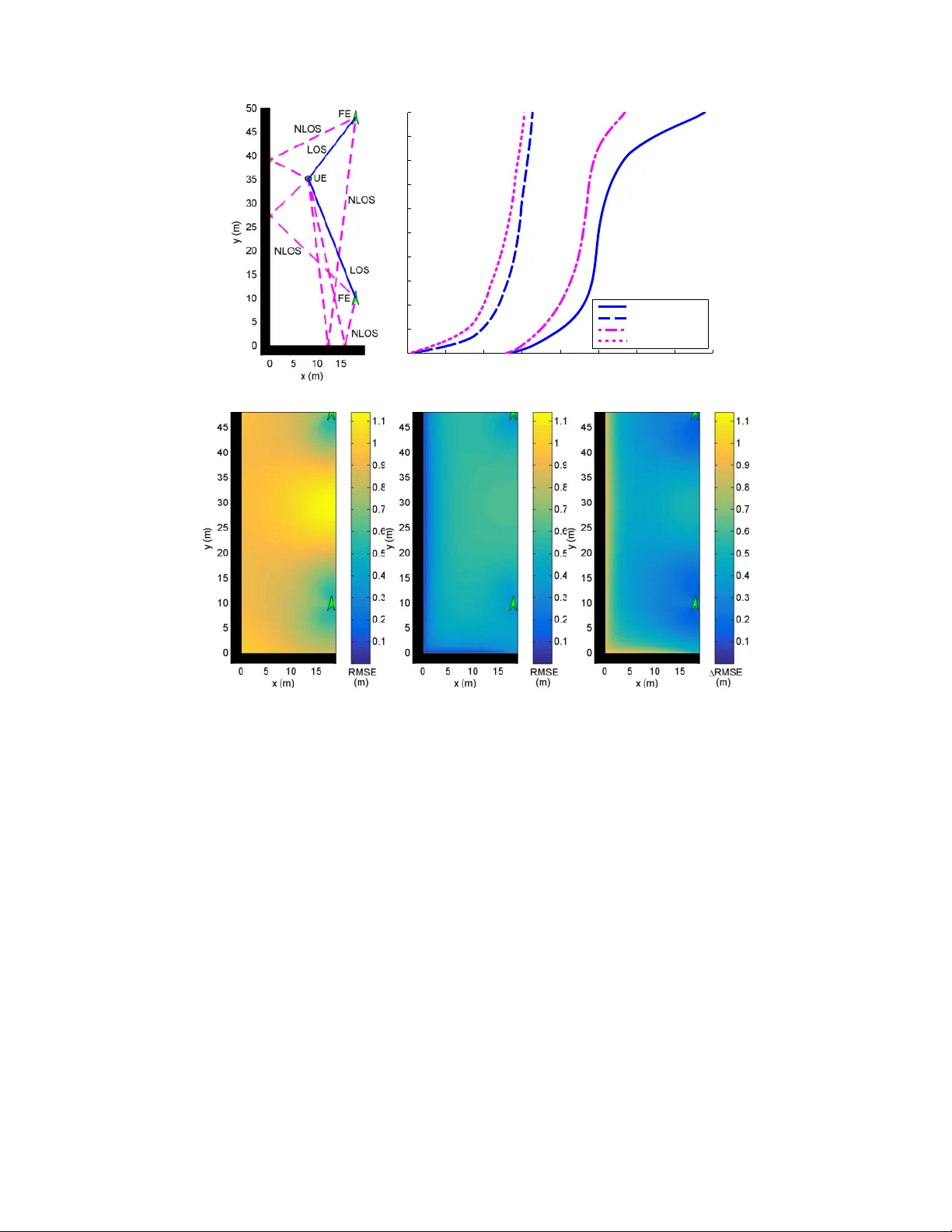
Loading comments...
Leave a Comment