Regression-based reduced-order models to predict transient thermal output for enhanced geothermal systems

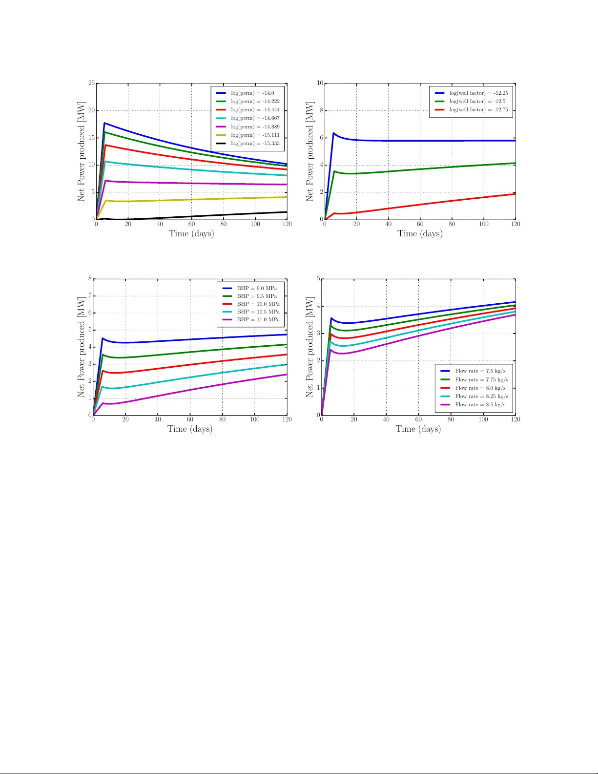
Regression-based reduced-order mo dels to predict transien t thermal output for enhanced geothermal systems M. K. Mudun uru ∗ , S. Karra, D. R. Harp, G. D. Guthrie, and H. S. Visw anathan Earth and Environmen tal Sciences Division, Los Alamos National Laboratory , Los Alamos, NM 87545. Abstract Reduced-order mo deling is a promising approac h, as many phenomena can be describ ed b y a few parameters/mec hanisms. An adv an tage and attractiv e asp ect of a reduced-order model is that it is computational inexp ensiv e to ev aluate when compared to running a high-fidelity n umerical sim ulation. A reduced-order mo del tak es couple of seconds to run on a laptop while a high-fidelit y sim ulation ma y tak e couple of hours to run on a high-p erformance computing cluster. The goal of this paper is to assess the utility of regression-based Reduced-Order Mo dels (ROMs) developed from high-fidelity n umerical simulations for predicting transient thermal p o w er output for an en- hanced geot hermal reserv oir while explicitly accoun ting for uncertainties in the subsurface system and site-sp ecific details. Numerical simulations are p erformed based on equally spaced v alues in the sp ecified range of mo del parameters. Key sensitiv e parameters are then iden tified from these simu- lations, which are fracture zone p ermeabilit y , well/skin factor, b ottom hole pressure, and injection flo w rate. W e found the fracture zone p ermeabilit y to b e the most sensitive parameter. The fracture zone permeability along with time, are used to build regression-based R OMs for the thermal pow er output. The ROMs are trained and v alidated using detailed physics-based numerical simulations. Finally , predictions from the R OMs are then compared with field data. W e prop ose three differen t R OMs with differen t levels of mo del parsimony , eac h describing key and essential features of the p o w er pro duction curv es. The co efficien ts in prop osed regression-based R OMs are dev elop ed b y minimizing a non-linear least-squares misfit function using Lev en b erg-Marquardt algorithm. The misfit function is based on the difference betw een n umerical simulation data and reduced-order mo del. R OM-1 is constructed based on p olynomials upto fourth order. ROM-1 is able to accurately repro duce the pow er output of numerical simulations for low v alues of p ermeabilities and certain features of the field-scale data. ROM-2 is a mo del with more analytical functions consisting of p oly- nomials upto order eight, exp onen tial functions and smo oth approximations of Heaviside functions, and accurately describ es the field-data. At higher permeabilities, ROM-2 reproduces numerical re- sults b etter than ROM-1, how ev er, there is a considerable deviation from numerical results at low fracture zone p ermeabilities. R OM-3 consists of p olynomials upto order ten, and is dev elop ed by taking the best aspects of ROM-1 and ROM-2. R OM-1 is relatively parsimonious than ROM-2 and R OM-3, while R OM-2 ov erfits the data. R OM-3 on the other hand, provides a middle ground for mo del parsimony . Based on R 2 -v alues for training, v alidation, and prediction data sets w e found 1 that R OM-3 is b etter mo del than ROM-2 and ROM-1. F or predicting thermal dra wdo wn in EGS applications, where high fracture zone p ermeabilities (typically greater than 10 − 15 m 2 ) are desired, R OM-2 and ROM-3 outp erform ROM-1. As p er computational time, all the R OMs are 10 4 times faster when compared to running a high-fidelit y numerical simulation. This mak es the prop osed regression-based ROMs attractive for real-time EGS applications b ecause they are fast and provide reasonably go od predictions for thermal p o wer output. Keyw ords: Enhanced Geothermal Systems (EGS), Reduced-Order Mo dels (R OMs), thermal draw- do wn, regression. 1. INTR ODUCTION AND PR OBLEM DESCRIPTION Enhanced Geothermal Systems (EGS) present a significant and long-term opp ortunity for wide- spread pow er production from new geothermal sources. EGS makes it p ossible to tap otherwise inaccessible thermal resources in areas that lack traditional geothermal systems. It is estimated that within the USA alone the electricity pro duction p oten tial of EGS is in excess of 100GW. Hence, the efforts to mo del and predict the p erformance of EGS reservoirs under v arious reservoir conditions (suc h as formation p ermeabilit y , reservoir temp erature, existing fracture/fault connectivit y , and in- situ stress distribution) are vital. In this pap er, we present a study based on reduced-order mo deling using data from the historic F en ton Hill Hot Dry Ro ck (HDR) pro ject [ 1 ]. F rom a practical p oin t of view, we are in terested in dev eloping fast mo dels to examine the p oten tial for supplying thermal energy at sustained rates for commercial op erations. Most of the existing studies related to EGS [ 2 – 18 ] are based on high-fidelity numerical simu- lations. These sim ulations are p erformed to gain detailed understanding of the physical pro cesses taking place in EGS reservoirs. How ev er, such detailed numerical simulations are computationally exp ensiv e as they tak e hours to run on h undreds of pro cessors, making them prohibitiv e for real- time applications. Herein, we shall take a different route to mo del and understand EGS systems based on reduced-order mo deling. Reduced-order mo dels are similar to analytical solutions. A ma jor adv antage of R OMs are that they tak e couple of seconds to run on a laptop as compared to high-fidelit y n umerical sim ulations. This makes them attractiv e for real-time and commercial applications. But the pro cedure to construct R OMs is differen t compared to constructing analytical solutions. In literature, they are v arious wa ys to dev elop reduced-order mo dels [ 19 – 24 ]. In our case, reduced-order mo dels are developed and trained based on high-fidelity numerical simulations. R OMs developed from high-fidelity numerical sim ulation data are not actual reduction of the ph ys- ical system but are pro xy/surrogate mo dels for certain quan tities of in terest such as thermal p o w er pro duction. As a result, there are no gov erning equations for such reduced-order mo dels. In the follo wing subsections, we briefly describ e the field exp erimen t and need for reduced-order mo dels. 1.1. A brief description of the problem and field exp erimen t. The aim of this pap er is to predict the thermal p o w er output during the Long-T erm Flow T est (L TFT) exp erimen t of Phase I I reservoir at the F enton Hill HDR test site, lo cated near Los Alamos, New Mexico [ 25 – 28 ]. This Phase I I reservoir was designed to test the HDR concept at temp eratures and thermal pro duction rates near those required for a commercial electrical p ow er plant [ 1 , 29 ]. One of the ob jectives of the curren t study is to include site-sp ecific conditions in developing mo dels. The op eration of L TFT experiment at F en ton Hill lasted for 39 months with 11 months of activ e circulation through the reserv oir. The Phase I I reservoir comprised of a single injection well 2 and single pro duction w ell. The injection pressure w as in the range of 25 MPa to 30 MP a and pro duction backpressure ranged from 8 MPa to 13 MPa. The injection and pro duction mass flow rates ranged from 7.5 kg s − 1 to 8.5 kg s − 1 and 5.5 kg s − 1 to 7.0 kg s − 1 . The injection and pro duction temp eratures at the well-head ranged from 293 K ( 20 o C ) to 303 K ( 30 o C ) and 438 K ( 165 o C ) to 458 K ( 185 o C ). Corresp ondingly , the b ottomhole temp eratures at the pro duction well accounting for friction loss are b etw een 453 K ( 180 o C ) and 498 K ( 225 o C ). F or more details on these data sets and other asp ects (such as tracer data, microseismic data, fracture netw orks, fracture connectivity , injection and pro duction wells en try p oin ts, and reactive-transport data), see References [ 1 , 29 ]. 1.2. Need for reduced-order mo dels. In recent y ears, mo del reduction tec hniques hav e pro ven to be p ow erful tools for solving v arious problems in geosciences. In reservoir managemen t and decision-making, R OMs are considered efficient yet p o werful tec hniques to address computational c hallenges asso ciated with managing realistic reserv oirs [ 30 ]. Examples of some popular research and scien tific endeav ors on reduced-order mo deling within the context of subsurface pro cesses include Cardoso et al. [ 19 , 20 ], He et al. [ 21 ], Pau et al. [ 22 ], and P asetto et al. [ 23 ]. Lo osely sp eaking, the problem of mo del reduction is to replace a detailed physics-based mo del of a complex system (or a set of processes) by a muc h “simpler” and more computationally efficien t mo del than the original mo del while still accurately predicting those aspects of the system that are of interest. There are sev eral reasons ROMs are useful in the con text of EGS, including: I R OMs facilitate in dev eloping site-sp ecific mo dels which are fast to compute. In general, they can b e also used as a substitute mo del for parameter estimation instead of in verse mo deling, which ma y require rep eated ev aluation of forw ard mo dels. I R OMs can b e used as n umerical surrogates to p erform detailed sensitivit y analysis and parametric studies, thereb y reducing the ov erall computational burden of high-fidelity nu- merical sim ulations. I In many-query applications suc h as EGS, a simple, efficient and predictiv e mo del is required for field use. Such a model can greatly reduce (or minimize) the associated op erational costs, thereb y maximizing the EGS p o w er output p oten tial. The ROMs developed in this pap er are based on regression. They are a com bination of p oly- nomials of different degrees, sin usoidal function, exponential function, and logistic function. The co efficien ts of these p olynomials and functions are obtained b y training the ROMs on high-fidelity n umerical simulation data. 1.3. Ob jectives and outline of the pap er. Among the v arious p oten tial outputs of interest from a full-physics based simulation for the challenge problem is the thermal p o w er pro duced. The ob jective of the study is to dev elop R OMs fo r an EGS to predict thermal p o wer output. W e are interested in developing a fast and predictive ROM for thermal p o w er output that accurately repro duces detailed simulations. T o achiev e this, the o verall approach inv olv es obtaining thermal p o w er data from detailed physics-based 3D numerical sim ulations using the parallel subsurface flow sim ulator PFLOTRAN [ 31 ]. Approximate range of mo del input parameters are constructed based an educated guess of the fractured EGS system (see Kelk ar et al. [ 29 , Section-3]). W e use equally spaced v alues of the input parameters to generate p o wer data for several cases. The R OMs are constructed, trained and v alidated against PFLOTRAN numerical sim ulations. These ROMs are then used to predict thermal p ow er output and compared with a field thermal p o wer data set from L TFT F en ton Hill HDR Phase I I exp erimen t. 3 The pap er is organized as follows: Section 2 describ es the physics-based conceptual mo del, which appro ximately models the F en ton Hill HDR Phase I I reservoir. It also provides a brief ov erview of the go verning equations for fluid flo w, thermal drawdo wn, and numerical metho dology to solv e the coupled conserv ation equations. Assumptions in mo deling these systems are also outlined. In Section 2 , w e also p erform calibration of the material parameters using the field thermal output data. These v alues serve as base case for the parameters. Using a range of v alues around these base case v alues, sensitiviy analysis is p erformed using PFLOTRAN and is shown in Section 2 . W orkflow for R OM developmen t is also describ ed in this section as well. Section 3 details a pro cedure to construct R OMs for thermal p o wer output. Details of training and v alidation are provided in this section as w ell. Predictive capabilities of R OMs with resp ect to thermal p o w er output and comparison against field-data is also discussed. Finally , conclusions are drawn in Section 4 . 2. CONCEPTUAL MODEL, GOVERNING EQUA TIONS, AND NUMERICAL METHODOLOGY In this section, w e briefly describ e the detailed n umerical sim ulations we used in the developmen t of the R OMs, including those gov erning equations needed to mo del physical pro cesses inv olv ed in heat extraction within a jointed reservoir. W e then present a physics-based conceptual mo del for an EGS reserv oir and corresp onding b oundary conditions. Finally , we describ e a n umerical metho d- ology to solv e the system of coupled partial differential equations using the subsurface simulator PFLOTRAN. PFLOTRAN solv es a system of nonlinear partial differential equations describing m ultiphase, multicomponent, and m ultiscale reactiv e flow and transp ort in p orous materials using finite volume metho d. Here, we shall restrict to solving the gov erning equations resulting for single phase fluid (w ater) flow and heat transfer pro cesses. 2.1. Go v erning equations: Fluid flo w and heat transfer. In order to predict the heat extraction pro cess, we solv e the following set of go verning equations. This includes balance of mass and balance of energy for fluid flow and thermal dra wdo wn. The gov erning mass conserv ation equation for single phase saturated flow is given by: ∂ ϕρ ∂ t + div[ ρ q ] = Q w (2.1) where ϕ is the p orosit y , ρ is the fluid density [kmol m − 3 ] , q is the Darcy’s flux [m s − 1 ] , and Q w is the v olumetric source/sink term [kmol m − 3 s − 1 ] . The Darcy’s flux is given as follows: q = − k µ grad[ P − ρg z ] (2.2) where k is the intrinsic p ermeabilit y [m 2 ] , µ is the dynamic viscosity [Pa s] , P is the pressure [Pa] , g is the gravit y [m s − 2 ] , and z is the v ertical comp onen t of the p osition vector [m] . The source/sink term is giv en as follows: Q w = q M W w δ ( x − x ss ) , where q M = Γ well ρ µ ( P − P bhp ) (2.3) where q M is the mass flo w rate [kg m − 3 s − 1 ] , W w is the formula weigh t of water [kg kmol − 1 ] , Γ well denotes the skin/w ell factor (which regulates the mass flow rate in the pro duction well) [unit-less], x ss denotes the lo cation of the source/sink, P bhp is the b ottom hole pressure of the pro duction well, 4 and δ ( • ) denotes the Dirac delta distribution [ 32 ]. The gov erning equation for energy conserv ation to mo del thermal drawdo wn and corresp onding heat extraction pro cesses is giv en as follows: ∂ ∂ t ( ϕρU + (1 − ϕ ) ρ rock c p,rock T ) + div [ ρ q H − κ grad[ T ]] = Q e (2.4) where U is the internal energy of the fluid, ρ rock is the true density of the ro c k (or ro c k grain density), c p,rock is the true heat capacity of the ro c k (or rock grain heat capacity), T is the temp erature of the fluid, H is the en thalpy of the fluid, κ is the thermal conductivity of p orous ro c k, and Q e is the source/sink term for heat extraction. 2.2. Ph ysics-based conceptual mo del: EGS reserv oir. W e shall briefly describ e the ph ysics- based conceptual mo del used in the n umerical sim ulation of Phase II F enton Hill HDR reservoir here. It should b e noted that this conceptual mo del is an approximation of a more complex sys- tem (see the References by Kelk ar et al. [ 29 ] and Brown et al. [ 1 ] for a detailed description of the reservoir). Suc h an approximation is performed to understand the essen tial features and con- struct a mo del that is amenable for numerical sim ulations. Figure 1 provides a pictorial description of the reserv oir. The reference datum, whic h is the reserv oir top surface, is appro ximately lo- cated at a depth of 3000 m . The dimensions and volume of the reserv oir are tak en to b e equal to 1000 × 1000 × 1000 m 3 . The fracture zone is an appro ximate representation of the region containing join t netw orks (fracture netw orks) and lo w-p ermeable p orous ro c k, whose dimensions are taken to b e around 650 × 650 × 500 m 3 . The fracture zone starting and ending co ordinates are approximately tak en to b e (200 m , 200 m , 200 m) and (850 m , 850 m , 700 m) . The injection and production wells are lo cated at around (575 m , 575 m , 450 m) and (675 m , 500 m , 625 m) . The distance b et w een the w ells b eing 215.06 m . These are idealized as v olumetric source/sink terms in performing the n u- merical simulations. Reserv oir and fracture zone p orosities are assumed to b e equal to 0.0001 and 0.1. The reservoir ro c k density , ro c k sp ecific heat capacit y , ro c k thermal conductivity , ro ck p erme- abilit y , fluid heat capacity , fluid density , and fluid injection temp erature are taken as 2716 kg m − 3 , 803 J kg − 1 K − 1 , 2.546 W m − 1 K − 1 , 10 − 18 m 2 , 4187 J kg − 1 K − 1 , 950 kg m − 3 , and 298 K (Note that the abov e system and material parameters are tak en from the Reference Swenson et al. [ 8 , T able 1]). The initial reservoir conditions for the mo del are at a pressure of 13.2 MPa and temp erature of 503 K [ 29 , Section-3]. No flo w b oundary conditions are assumed for solving the flow equations. Zero gradien t b oundary conditions are assumed for solving heat transfer equations. Figure 2 shows the resp ectiv e injection pressure and pro duction backpressure, injection and pro duction mass flo w rates, injection and pro duction temp eratures, and thermal p o w er extracted during the Phase I I L TFT exp erimen t. These field data sets are extracted from the Hot Dry Ro c k Final Rep ort b y Kelk ar et al. [ 29 ]. T o get an estimate of the mo del parameters for the L TFT set-up, the mo del is calibrated against field-data. Lev en b erg-Marquardt (LM) Algorithm implemen ted in MA TK soft w are [ 33 ] along with PFLOTRAN is used to estimate the parameters – fracture zone p ermeabilit y , pro duction temp erature, bottom hole pressure, and skin/w ell factor. By v arying the parameters around the calibrated parameter v alues, sensitivity analysis is p erformed. Details are discussed in the next subsection. 2.3. Numerical metho dology. The go verning flo w and heat transfer equations are solv ed using the PFLOTRAN simulator, which employs a fully implicit bac kward Euler for discretizing time and a tw o-p oin t flux finite v olume metho d for spatial discretization [ 31 , App endix B]. The resulting 5 non-linear algebraic equations are solved using a Newton-Krylov solver. Numerical simulations are p erformed for t wo different scenarios (see Figure 3 ). Case #1: Calibration is based on constant injection flow rate, whic h is equal to 7 . 5 kg s − 1 1 . Case #2: Calibration is p erformed based on time- v arying injection flow rates, whose v alues are plotted in Figure 2 . In this case, the mean square error b et w een thermal p o wer output data based on PFLOTRAN numerical sim ulations and L TFT field-data is minimized using LM algorithm. The resulting parameters are given as follo ws: I F racture zone p ermeabilit y – Constan t injection: 7 . 75 × 10 − 16 m 2 – Time-v arying injection: 1 . 78 × 10 − 16 m 2 I Pro duction temp erature: 438 K ( 165 o C ), whic h is the same for b oth cases. I Bottom hole pressure: – Constan t injection: 9.5 MPa – Time-v arying injection: 9.42 MPa I Skin/w ell factor [unit-less] to regulate mass flow rate in pro duction well: – Constan t injection: 3 . 163 × 10 − 13 – Time-v arying injection: 5 . 37 × 10 − 13 The p o w er output from the n umerical simulation is calculated from the following expression: Net p o w er pro duced = ( Pro duction mass flow rate × Fluid heat capacity × Pro duction temp erature ) − ( Injection mass flow rate × Fluid heat capacity × Injection temp erature ) (2.5) Figure 3 shows the approximate fit of the PFLOTRAN n umerical simulation with the field-scale data of the p o w er output based on the parameters estimated for Case #1 and Case #2. The R 2 - v alues for Case #1 and Case #2 are equal to 0.74 and 0.68, which are close to eac h other. The mean square error (MSE) v alues for Case #1 and Case #2 are 0.603 and 0.018, which are considerably differen t. Reason b eing that the LM algorithm calibrates the mo del parameters b y minimizing the MSE v alue. It should b e noted that the calibrated parameters of the constan t injection flo w rate case and time-v arying injection flow rate case are of the same order, whic h is enough for p erforming sensitivit y analysis to identify k ey sensitiv e input parameters for ROMs construction. The next subsection describ es the w orkflow for ROM construction and the corresponding numerical studies on v arious mo del parameters [ 34 ]. 2.4. Sensitivit y analysis, ROM developmen t workflo w, and numerical results. In this subsection, w e p erform sensitivity studies on v arious input/output mo del parameters to mo del EGS reserv oirs. Suc h an analysis is p erformed to iden tify key sensitive parameters for ROM inputs. These mo del parameters include mass flow rate at the injection w ell, skin/w ell factor to regulate mass flo w rate in pro duction well, fracture zone p ermeabilit y , and b ottom hole pressure. Figure 4 shows the PFLOTRAN numerical sim ulation results for the ab o ve four key parameters. These figures are plotted for each sensitive parameter by keeping all other parameters fixed to base case calibrated v alues. F or example, if fracture zone p ermeabilit y is v aried from the base v alue (whic h is equal to 7 . 75 × 10 − 16 m 2 ), the other three estimated v alues for the parameters are k ept 1 It should b e noted that the inten t of L TFT exp erimen t is to inject fluid in to reservoir at a constant flow rate [ 1 , 29 ] so that geothermal energy could b e extracted at a sustained rate. Ho wev er, due to v arious op erational issues, near-constant flow rates were observed during 20 < t < 60 and 80 < t < 120 days. There seems to b e a breakthrough in injection flow rate from 0 < t < 20 due to wellbore breakouts [ 1 ]. 6 constan t. This is done to sho w, identify , and rank the k ey sensitive input parameters for the ROMs. Based on Figure 4 , it is apparent that the p o w er pro duction is highly sensitive to v arying fracture zone permeability and least sensitive to injection mass flow rates. Corresp ondingly , the skin/w ell factor to control mass flow rate in pro duction w ell and b ottom hole pressure (BHP) are second and third in sensitivity ranks after fracture zone p ermeabilit y . T o consolidate, the ranking of imp ortance of inputs for ROM developmen t are giv en as follows (in the decreasing order): (1) F racture zone p ermeabilit y (p o w er pro duction v aries in a non-linear fashion) (2) Skin/w ell factor to regulate mass flow rate in pro duction well (3) Bottom hole pressure (4) Injection mass flo w rate (p o wer pro duction v aries in a linear fashion) R OM dev elopment is summarized as a flow c hart in Figure 5 . The next section describ es an approach to construct R OMs for p o w er output. 3. REDUCED-ORDER MODELING The ob jectiv e of model reduction metho dologies is to use the kno wledge generated by high fidelit y and time-consuming numerical sim ulations to generate special functions that make use of prop erties of underlying systems, thereb y obtaining a go o d understanding of the phenomena of in terest. Subsection 1.2 discusses man y reasons why such a detail is warran ted. W e shall now pro vide an ov erview of some p opular mo del order reduction metho ds and algorithms. These techniques either use physical (or other) insight or sensitivity studies on model parameters as a basis to reduce the complexit y of the underlying problem and obtain a go o d approximation of the required output in an efficien t wa y . Some p opular mo del reduction metho ds include regression-based mo del order reduction [ 35 – 37 ], op erational mo del order reduction [ 38 , 39 ], compact reduced-order modeling [ 38 ], truncated bal- anced realization [ 40 ], optimal Hankel-norm mo del order reduction [ 41 ], Gaussian process regres- sion (GPR) [ 22 , 42 ], prop er orthogonal decomp osition (POD) [ 43 ], asymptotic wa v eform ev aluation (A WE) and its v arian ts [ 44 ], Pade via Lanczos (PVL) and its v arian ts [ 45 ], sp ectral Lanczos decom- p osition metho d (SLDM) [ 46 ], and truncation-based mo del order reduction [ 38 ]. F or more details on these methods, algorithms, and implemen tation asp ects (see References Qu, [ 47 ], Sc hilders et al. [ 38 ], Quarteroni and Rozza [ 48 ], and Mignolet et al. [ 49 ]). Here, w e shall construct reduced-order mo dels based on regression-based mo del order reduction metho ds, whic h result in simple thermal p o w er output R OMs. These ROMs consist of a set of algebraic relations that dep end on the k ey sensitiv e parameters (which is fracture zone p ermeabilit y) that can b e ev aluated very quickly . 3.1. Reduced-order mo dels for p o wer output based on regression-based metho ds. R OMs are constructed using a combination of p olynomials, trigonometric functions, exp onential functions, and smo oth approximation of step functions. Logistic functions are chosen as the smo oth- appro ximation of step functions. The rationale behind choosing suc h functions are as follo ws: P olynomials, trigonometric functions, and exp onen tial functions capture the in crease and decay part of the field-scale p o wer output data and PFLOTRAN numerical sim ulations, while the logistic functions are intended to capture the p eaks and sudden v ariations. The co efficien ts of these functions are constructed through a non-linear least-squares regression fit to the PFLOTRAN simulations. T o obtain the resp ectiv e co efficien ts of the functions in the R OMs, non-linear least-squares regression w as p erformed using the optimization solvers a v ailable in the op en-source Python pack age Scipy [ 50 ]. 7 Belo w we pro vide a summary of ROMs construction. It should b e noted that all of the simulation data from the sensitivity analysis is used to train and v alidate the ROMs: • T raining data from PFLOTRAN simulations is used to construct all ROMs. These simu- lations are p erformed for log(p ermeabilit y) v alues equal to -14.0, -14.444, -14.667, -14.889, and -15.333. • F or R OM-2, in addition to abov e training datasets, a small subset of field-scale data is used to construct the ROM. These include the L TFT field thermal p o wer data at times t = 0 , 20 , 25 , 40 , 60 , 80 , 100 , and 120 . • F or v alidation, the PFLOTRAN sim ulations p erformed at log(p ermeabilit y) v alues equal to -14.222 and -15.111 are used. • F or prediction, the L TFT thermal p o w er output field data is used. • R OM-1 is constructed using p olynomials of order upto degree four. ROM-2 is constructed using polynomials of order upto degree eight, sine function, exp onen tial function, and smo oth approximation of Hea viside functions. R OM-3 is constructed using p olynomials of order upto degree ten. • The co efficien ts of the R OMs are determined by minimizing the sum of squares of nonlinear functions. This is achiev ed b y using Scipy library’s non-linear least-squares fit function called “ scipy.optimize.curve-fit ”. • Using the developed ROMs, the R 2 -v alues are then calculated for training, v alidation, and prediction data. It should b e noted that a small subset of field data is used to train a particular R OM, which is R OM- 2. At these v alues, w e exactly repro duce field thermal p o w er output for calibrated permeability v alue. Ho w ev er, other R OMs are not trained using the observ ation data. Observ ation data is first used to obtain realistic parameter range to generate the sim ulation datasets. These simulation datasets are then used to dev elop the ROMs. Figure 3 sho ws the calibration to obtain the base case parameter v alues for the simulation datasets. The parameters used here include fracture zone p ermeabilit y , bottom hole pressure, and w ell factor. Then, based on a sensitivity analysis study , w e found the fracture zone p ermeabilit y to b e the most sensitive parameter and so the R OMs were constructed as a function of time and p ermeabilit y . Next, we prop ose and discuss three regression-based reduced-order mo dels with different levels of mo del parsimony . Algorithm 1 provides a detailed description of the prop osed regression-based R OMs construction. Eac h mo del has it own pros and cons, which are describ ed b elo w: 3.1.1. Thermal p ower output ROM-1 . P ow er rom-1 = a 0 ( t ) + 3 X i =1 a i ( t )  | log( k fz ) | + 10 − 6 t  i (3.1) where t denotes the time in days, the co efficien ts a i are function of time (da ys), and k fz is the fracture zone p ermeabilit y . 3.1.2. Thermal p ower output ROM-2 . P ow er rom-2 = b 0 ( t ) + 3 X i =1 b i ( t )  | log( k fz ) | + 10 − 6 t  i + 29 X j =1 m j (1 + tanh( n j ( t − t j ))) r j | {z } Smooth approximation of Heaviside function (3.2) 8 T able 1. Summary of prop osed reduced-order mo dels for thermal p o wer output. A small subset of field-scale data is used to construct the ROM-2. These include the L TFT field thermal p o wer data at times t = 0 , 20 , 25 , 40 , 60 , 80 , 100 , and 120 . Model Thermal Po w er Output ROM-1 a 0 ( t ) + 3 X i =1 a i ( t )  | log( k fz ) | + 10 − 6 t  i ROM-2 b 0 ( t ) + 3 X i =1 b i ( t )  | log( k fz ) | + 10 − 6 t  i + 29 X j =1 m j (1 + tanh( n j ( t − t j ))) r j ROM-3 c 0 ( t ) + 3 X i =1 c i ( t )  | log( k fz ) | + 10 − 6 t  i T able 2. R 2 -v alues for training, v alidation, and prediction of numerical simulations and L TFT field-data. Out of total sev en sim ulation datasets, 5 were used for training and 2 for v alidation. T o construct training dataset, n umerical sim ulations are performed for log(p ermeabilit y) v alues equal to -14.0, -14.444, -14.667, -14.889, and -15.333. T o construct v alidation dataset, n umerical sim ulations are performed for log(permeability) v alues of - 14.222 and -15.111. Prediction dataset b eing the L TFT thermal p o wer output field-data. Model R 2 -v alues T raining V alidation Prediction ROM-1 0.489, 0.326, 0.22, 0.75, and 0.96 0.406 and 0.407 0.668 ROM-2 0.877, 0.804, 0.796, 0.689, and 0.573 0.817 and 0.542 0.986 ROM-3 0.917, 0.896, 0.9, 0.889, and 0.813 0.892 and 0.893 0.824 3.1.3. Thermal p ower output ROM-3 . P ow er rom-3 = c 0 ( t ) + 3 X i =1 c i ( t )  | log( k fz ) | + 10 − 6 t  i (3.3) The ab o v e ROMs are used to predict L TFT thermal p o w er output data as function of time and fracture zone p ermeabilit y . As p er computational cost, the time taken to run a PFLOTRAN sim ulation is around 45 seconds. T o construct the regression ROMs described ab ov e w e need 5 high-fidelit y simulations for training and 2 high-fidelity simulations for v alidation. Hence, the total time taken to run 7 high-fidelity sim ulations is around 315 seconds. T o construct ROM-1, R OM-2, and R OM-3, w e need to find coefficients of a i ( t ) , b i ( t ) , and c i ( t ) . The co efficien ts of the R OMs are obtained by minimizing the sum of squares of nonlinear functions with resp ect to training data using Leven berg-Marquardt algorithm. The procedure to obtain these co efficien ts is describ ed in Algorithm 1 and the co efficien t v alues are given in App endix. The Leven berg-Marquardt algorithm tak es around 0.06, 0.16, and 0.1 seconds to obtain the co efficien ts of ROM-1, ROM-2, and ROM-3. The time taken by ROM-1, R OM-2, and R OM-3 to make a prediction is around 0.0002, 0.0015, and 0.0008 seconds. This means the ROMs are 10 4 times faster than a high-fidelit y numerical sim ulation. Remark 3.1 . The r e gr ession-b ase d ROMs ar e sp e cific to this EGS applic ation. The pr op ose d R OMs c an b e gener alize d by r emoving site-sp e cific asp e cts in ROMs c onstruction in Algorithm 1 . 9 Algorithm 1 A numerical metho dology to construct regression-based reduced-order mo dels for EGS 1: INPUT s for PFLOTRAN sim ulations: F racture zone permeability , bottom hole pressure, w ell factor, and injection flow rate. 2: T o construct regression-based ROMs, get high-fidelity n umerical simulation data b y running PFLOTRAN sim ulator for different parameter v alues. T otal n umber of simulations = 2625. • Logarithm of fracture zone p ermeabilit y = − 14 . 0 , − 14 . 222 , − 14 . 444 , − 14 . 667 , − 14 . 889 , − 15 . 111 , − 15 . 333 . • Logarithm of well factor = − 12 . 25 , − 12 . 5 , − 12 . 75 . • Bottom hole pressure = 9 . 0 , 9 . 5 , 10 . 0 , 10 . 5 , 11 . 0 . • Injection mass flow rate = 7 . 5 , 7 . 75 , 8 . 0 , 8 . 25 , 8 . 5 . 3: Post-process each high-fidelity numerical simulation to obtain thermal p o w er output as function of time. Then, p erform sensitivity analysis and iden tify the dominant parameter. In our case, w e found fracture zone p ermeabilit y is dominan t. See Subsection 2.4 for more details. 4: The prop osed regression-based ROMs are function of time and dominant parameter, which is fracture zone p ermeabilit y . See Equations ( 3.1 )–( 3.3 ). 5: T o construct, train, and v alidate ROMs, among 2625 high-fidelity simulation dataset we choose a subset with v arying fracture zone permeability (while other parameters are k ept constant). The v alues of the other parameters corresp ond to the calibration case. • Calibration case parameter v alues are: Logarithm of w ell factor = − 12 . 5 , b ottom hole pressure = 9 . 5 , and injection mass flow rate = 7 . 5 . • There are a total of 7 PFLOTRAN simulations that are used in the proposed ROM construction metho dology . Out of 7 simulations, 5 simulations are used for training and 2 simulations are used for v alidation of ROMs. L TFT thermal p o w er output data is used for prediction. 6: ROM-1 construction: a 0 ( t ) + 3 X i =1 a i ( t )  | log( k fz ) | + 10 − 6 t  i • Polynomials of order upto degree four are selected. • The co efficien ts in a i ( t ) are obtained my minimizing the error b et w een high-fidelity sim ulation data and the explicit expression of ROM-1. • The co efficient v alues, which are obtained by solving the non-linear least-squares re- gression using Lev enberg-Marquardt algorithm are given b y Equations ( 4.1a )–( 4.1d ). 7: ROM-2 construction: b 0 ( t ) + 3 X i =1 b i ( t )  | log( k fz ) | + 10 − 6 t  i + 29 X j =1 m j (1 + tanh( n j ( t − t j ))) r j • Polynomials of order upto degree eigh t, sine, exp onential, and smo oth approximation of Hea viside functions are selected. • The non-linear least-squares regression problem is solved with the constrain t that at times t = 0 , 20 , 25 , 40 , 60 , 80 , 100 , and 120 , the R OM-2 mo del output matches the L TFT thermal p o w er output data. The co efficients are giv en by Equations ( 4.2a )–( 4.4j ). 8: ROM-3 construction: a 0 ( t ) + 3 X i =1 a i ( t )  | log( k fz ) | + 10 − 6 t  i • Polynomials of order upto degree ten are selected. R OM-3 is constructed in similar fashion to ROM-1. The co efficien t v alues in c i ( t ) are given by Equations ( 4.5a )–( 4.5d ). 9: OUTPUTS: Regression mo dels for ROM-1, R OM-2, and R OM-3. Mo del expressions are given in App endix. They are used to predict thermal p ow er output. 10 These include, r elaxing the r ange of inje ction r ates, wel l factor values, b ottom hole pr essur es, and fr actur e zone p erme ability. F or a new site, first we ne e d to c onstr ain the p ar ameter sp ac e sp e cific to that site. Then, we just have to use the same metho dolo gy pr op ose d in Algorithm 1 to c onstruct r e gr ession-b ase d ROMs sp e cific to the new site. 3.2. Discussion and inferences: Predictive capabilities of R OMs with resp ect to field-scale data and PFLOTRAN. W e shall now pro vide a rationale b ehind the construction of these R OMs. Moreo ver, w e shall analyze the capabilities of these three R OMs in describing the trends in field-scale data and PFLOTRAN sim ulations. The construction of ROM-1 is purely based on p olynomials. This ROM consists of p ow er-series terms (up to order four) inv olving natural log- arithm of fracture zone p ermeabilit y and time. The co efficien ts of the ROM-1 are constructed by matc hing the p o w er output of PFLOTRAN numerical simulations at certain fixed interv als of time (for v arious fracture zone p ermeabilities). Figure 6 sho ws the training, v alidation using n umerical sim ulations of ROM-1 along with its predictions. The predictions are compared with field pow er data. The b eha vior of ROM-1 is clearly distinct from the PFLOTRAN predictions (i.e., PFLO- TRAN predicts a rapid increase in the first few days follo wed b y a smo oth decline ov er the rest of the time p eriod, whereas ROM-1 shows a more gradual rise follow ed by a v arying decline). Nevertheless, for time p erio ds b et w een 20-100 days, ROM-1 is able to accurately repro duce the p ow er output of n umerical simulations for lo w v alues of fracture zone permeability . How ev er, as the fracture zone p ermeabilit y increases, there is a considerable deviation b et w een ROM-1 outputs and PFLOTRAN n umerical sim ulations. This is b ecause ROM-1 is constructed by matching PFLOTRAN n umerical sim ulations only at certain time in terv als. Moreov er, the p olynomial order considered to construct the R OM is very low. In terms of predicting the field-scale data, ROM-1 is able to repro duce only certain qualitative features of the field-scale data (Figure 6 ) and is relatively parsimonious. These asp ects include the initial increase of pow er output, the corresp onding decrease after the time t = 20 da ys, and then an increase in the p o wer output after t = 100 da ys. How ev er, quan titativ ely , the difference in p o wer output v alues of ROM-1 and L TFT exp erimen t are high. Figure 7 shows the b eha vior of R OM-2. F rom equation ( 3.2 ), it is evident that R OM-2 has more num b er of terms and co efficien ts than R OM-1. The motiv ation b ehind the construction of suc h a mo del is that we would like to accurately describ e the L TFT exp eriment at v arious time in terv als. ROM-2 is constructed by adding smo oth approximations of step functions and higher-order p olynomials to ROM-1. Figure 7 shows the training and v alidation against numerical simulations and final predictions of R OM-2. The predictions are compared with L TFT exp eriment. F rom this figure, it evident that R OM-2 shares some of the limitations of R OM-1: It does not repro duce the rapid rise in net p o wer pro duced for the initial days of operation (alb eit the fit is better than ROM-1), nor do es it repro duce a nearly linear decline for times out to 120 days. R OM-2 qualitativ ely repro duces the decline p ortion of the PFLOTRAN predictions (for da ys 20-120), but it ov er predicts the n umerical simulations, quan titatively . In general, ROM-2 repr o duces the PFLOTRAN results better than R OM-1 at higher p ermeabilities. Interestingly , p o w er output predicted using R OM-2 closely matches the L TFT exp erimen t, qualitativ ely and quantitativ ely . How ev er, R OM-2 is ov erfitted (see T able 2 for R 2 -v alues). In terms of repro ducing the field-scale data and PFLOTRAN simulations at higher p ermeabilit y ROM-2 is certainly b etter than ROM-1. Motiv ated by these tw o ROMs, ROM-3 is constructed. The philosoph y of ROM-3 is to use only p olynomials. The num b er of terms is determined by the co efficien t v alues. The maxim um p ossible 11 order for the p olynomial chosen is 10. This is b ecause as the order of p olynomial increases the v alues of the co efficien t are close to machine precision (close to zero). Figure 8 shows the training, v alidation using n umerical simulations of ROM-3 along with its predictions. The predictions are compared with field p o wer data. F rom this figure (8a/9a), it is apparent that R OM-3 more accurately repro duces the trend in the b eha vior of thermal p o wer output than ROM-2. F or numerical sim ulations, as the p ermeabilit y increases the deviations in the output v alues of R OM-3 and PFLOTRAN n umerical sim ulations are not very large as compared to R OM-1 and R OM-2. In the case of the L TFT exp erimen t, R OM-3 is able to accurately describ e the increase in the thermal p o w er output in initial stages. After time t = 20 days, when compared to the p erformance of R OM-2, ROM-3 is not exactly a close match to the L TFT data quantitativ ely . How ev er, qualitatively , R OM-3 is a m uch b etter mo del compared to ROM-1 due to the incorp oration of higher-order p olynomials (see T ables 1 and 2 for more details). In short, ROM-3 neither ov erfits nor underfits the L TFT exp erimen t data. Hence, ROM-3 is a b etter mo del compared to R OM-2 and ROM-1 and pro vides a middle ground for mo del parsimon y . The mo del can b e impro ved by incorp orating other input terms such as well factor, b ottom hole pressure, and injection mass flow rates. This is b ey ond the scop e of the curren t pap er and will b e considered in our future w ork. T able 1 summarizes the ROMs and their R 2 -v alues for training, v alidation, and prediction of numerical simulati ons and L TFT field-data. T o conclude the discussion, the follo wing can b e inferred based on Figures 6 – 8 and equations ( 3.1 )–( 4.5d ): I In repro ducing PFLOTRAN numerical sim ulations, for low v alues of p ermeability , R OM-1 outp erforms ROM-2 and R OM-3. At higher v alues of p ermeabilit y , R OM-2 outp erforms R OM-1 and ROM-3. In predicting L TFT data, ROM-2 outp erforms ROM-3 and ROM-1. Ho wev er, R OM-3 is able to describ e the initial trend in the field-data and other qualitative asp ects (such as the rise in p o wer pro duction after t = 10 da ys and decline after t = 30 da ys). I A t first glance, it may seem that ROM-2 may be the b est mo del in reproducing L TFT data. Ho wev er, from Figure 7 , it is eviden t that ROM-2 considerably deviates from the PFLOTRAN sim ulations at low v alues of p ermeabilit y . T ypically , for EGS applications, higher effective fracture zone p ermeabilities are desired [ 1 ]. This is b ecause in man y practi- cal scenarios (assuming that reserv oir matrix p ermeabilit y to b e very low), higher fracture zone p ermeabilities can b e correlated to (p ossibly) well connected and disp ersed discrete fracture netw orks [ 51 ]. This means that the fluid sweeps through a larger fractured volume (as compared to low er fracture zone permeabilities) resulting in higher p o wer pro duction at pro ducing w ells. T o mo del such scenarios, w e believe ROM-2 and ROM-3 are better mo dels than ROM-1. 4. CONCLUDING REMARKS In this pap er, we hav e presented v arious reduced-order mo dels to describ e different asp ects of the n umerical simulations and L TFT field-scale p o wer output data of Phase I I F enton hill geothermal reserv oir. First, w e describ ed the go verning equations for fluid flo w in the fractured reserv oir and corresp onding thermal drawdo wn. Second, we hav e presented a physics-based conceptual mo del for an EGS reservoir. The conceptual mo del is an appro ximation of a more complex system, which is used to understand the essential features of the systems and make it amenable for numerical simu- lations. Field-scale data sets, which are extracted from the do cumen ts provided by the geothermal 12 co de comparison pro ject, are used to estimate the parameters of the EGS system under considera- tion. These data sets include pressures, bac kpressures, mass flow rates, and temp eratures at b oth injection and pro duction sites. Third, sensitivity analysis is p erformed on these inputs to iden tify and rank the k ey parameters: fracture zone p ermeabilit y , well factor, injection flow rate and b ottom hole pressure. Based on this analysis, fracture zone permeability was found to be most imp ortant and so we used only p ermeability and time as the parameters for ROM construction. Finally , the R OMs are developed using the numerical simulations obtained based on equally spaced parametric v alues. The R OMs are built (trained and v alidated) using simulation data from the numerical model (PFLOTRAN) as shown in Figures 6 , 7 , and 8 . Then, these ROMs are used to predict the b eha vior of an EGS system, sp ecifically , F en ton Hill system. The input to these R OMs are p ermeabilit y and time. F rom the calibration in Figure 4, w e first obtain the p ermeabilit y of the F enton Hill EGS system. This p ermeabilit y v alue along with time are then used in ROM predictions, and compared with the observ ation data to ev aluate the p erformance of the ROMs. W e ev aluated three differen t ROMs with differen t lev els of mo del parsimon y , eac h describing k ey and essential features of the L TFT p o wer output data. The first ROM is a simple mo del and is able to accurately describ e the p o w er output at lo w fracture zone p ermeabilities, and is relativ ely parsimonious. The second R OM is a more complex mo del than R OM-1. Ho wev er, ROM-2 shares some of the limitations of R OM-1. In general, ROM-2 repro duces the numerical simulations b etter than R OM-1 at higher p ermeabilities. The in teresting part of ROM-2 is that the pow er output predicted closely matches the L TFT exp erimen t, qualitatively and quantitativ ely . The third ROM is constructed b y taking the b est asp ects of ROM-1 and ROM-2, and pro vides a middle ground for mo del parsimony . ROM-3 is able to quan titativ ely and qualitatively describ e the trend in the p o w er output at differen t time levels for b oth PFLOTRAN numerical simulations and L TFT p o wer output data. F rom these ROM developmen t workflo ws and sensitivity analyses, it is eviden t that this study has demonstrated that simple reduced-order models are able to capture v arious complex features in the system. This work provides confidence in dev eloping simple and efficient transien t reduced- order mo dels for geothermal field use. F or EGS applications, higher fracture zone p ermeabilit y is desired [ 1 ]. This is b ecause at higher p ermeabilities p o wer output is higher as the fluid sw eeps through a larger fracture zone volume. F or suc h scenarios (at higher p ermeabilities in predicting the thermal p ow er pro duction), ROM-2 and ROM-3 outp erform R OM-1. W e think R OM-2 and R OM-3 show promise for EGS studies. APPENDIX The co efficien ts for ROM-1 are given as follows: a 0 ( t ) = − 2 . 689 × 10 3 − 9 . 951 × 10 2 t + 28 . 37 t 2 − 3 . 013 × 10 − 1 t 3 + 1 . 095 × 10 − 3 t 4 (4.1a) a 1 ( t ) = 5 . 517 × 10 2 + 2 . 01 × 10 2 t − 5 . 751 t 2 − 6 . 111 × 10 − 2 t 3 − 2 . 222 × 10 − 4 t 4 (4.1b) a 2 ( t ) = − 3 . 718 × 10 1 − 1 . 347 × 10 1 t + 3 . 867 × 10 − 1 t 2 − 4 . 112 × 10 − 3 t 3 + 1 . 495 × 10 − 5 t 4 (4.1c) a 3 ( t ) = 8 . 241 × 10 3 + 2 . 998 × 10 − 1 t − 8 . 634 × 10 − 3 t 2 + 9 . 184 × 10 − 5 t 3 − 3 . 339 × 10 − 7 t 4 (4.1d) 13 F or R OM-2, the co efficien ts b i are functions of time (days), which are given as follows: b 0 ( t ) = 2 . 318 × 10 3 − 2 . 466 × 10 3 t + 1 . 338 × 10 2 t 2 − 3 . 413 t 3 + 4 . 612 × 10 − 2 t 4 − 3 . 393 × 10 − 4 t 5 + 1 . 376 × 10 − 6 t 6 − 3 . 538 × 10 − 9 t 7 + 6 . 869 × 10 − 12 t 8 − 2 . 307 × 10 3 × (0 . 1) t + 1 . 342 sin( t ) (4.2a) b 1 ( t ) = − 4 . 623 × 10 2 + 4 . 992 × 10 2 t − 2 . 713 × 10 1 t 2 + 6 . 918 × 10 − 1 t 3 − 9 . 339 × 10 − 3 t 4 + 6 . 856 × 10 − 5 t 5 − 2 . 766 × 10 − 7 t 6 + 7 . 056 × 10 − 10 t 7 − 1 . 369 × 10 − 12 t 8 − 2 . 307 × 10 3 × (0 . 1) t − 2 . 676 sin( t ) (4.2b) b 2 ( t ) = 3 . 103 × 10 1 − 3 . 353 × 10 1 t + 1 . 825 t 2 − 4 . 652 × 10 − 2 t 3 + 6 . 28 × 10 − 4 t 6 − 4 . 608 × 10 − 6 t 5 + 1 . 858 × 10 − 8 t 6 − 4 . 734 × 10 − 11 t 7 + 9 . 191 × 10 − 14 t 8 − 3 . 087 × 10 1 × (0 . 1) t + 1 . 796 × 10 − 2 sin( t ) (4.2c) b 3 ( t ) = − 6 . 997 × 10 − 1 + 7 . 477 × 10 − 1 t − 4 . 073 × 10 − 2 t 2 + 1 . 038 × 10 − 3 t 3 − 1 . 402 × 10 − 5 t 4 + 1 . 031 × 10 − 7 t 5 − 4 . 168 × 10 − 10 t 6 − 1 . 068 × 10 − 12 t 7 − 2 . 073 × 10 − 15 t 8 + 6 . 964 × 10 − 1 × (0 . 1) t − 4 . 048 × 10 − 4 sin( t ) (4.2d) The parameters t j (da ys) are c hosen in suc h a w ay that the R OM outputs b e close to that of the field-scale L TFT thermal pow er output at the i -th time-snapshots/time-lev els. These time v alues are giv en as follows: t 1 = 10 , t 2 = 15 , t 3 = 17 . 5 , t 4 = 19 , t 5 = 20 , t 6 = 21 , t 7 = 22 . 5 , t 8 = 25 , t 9 = 30 , t 10 = 32 . 5 (4.3a) t 11 = 35 , t 12 = 37 . 5 , t 13 = 50 , t 14 = 52 . 5 , t 15 = 55 , t 16 = 60 , t 17 = 62 . 5 , t 18 = 65 , t 19 = 70 , (4.3b) t 20 = 75 , t 21 = 80 , t 22 = 85 , t 23 = 87 . 5 , t 24 = 90 , t 25 = 95 , t 26 = 100 , t 27 = 105 , (4.3c) t 28 = 110 , t 29 = 112 . 5 (4.3d) The co efficien ts m j , n j , r j are giv en as follows: m 1 = 0 . 1 , m 2 = 0 . 085 , m 3 = 0 . 05 , m 4 = − 0 . 0125 , m 5 = 0 . 125 , m 6 = 0 . 1 , m 7 = − 0 . 0125 (4.4a) m 8 = 0 . 085 , m 9 = − 0 . 075 , m 10 = − 0 . 085 , m 11 = 0 . 085 , m 12 = 0 . 125 , m 13 = − 0 . 085 , (4.4b) m 14 = − 0 . 01 , m 15 = − 0 . 05 , m 16 = − 0 . 075 , m 17 = − 0 . 075 , m 18 = − 0 . 025 , m 19 = − 0 . 015 , (4.4c) m 20 = − 0 . 15 , m 21 = − 0 . 05 , m 22 = − 0 . 05 , m 23 = − 0 . 05 , m 24 = − 0 . 15 , m 25 = − 0 . 1 , (4.4d) m 26 = − 0 . 085 , m 27 = − 0 . 175 , m 28 = − 0 . 05 , m 29 = 0 . 05 , (4.4e) n 1 = n 2 = n 3 = 100 , n 4 to n 29 = 1000 (4.4f ) r 1 = r 2 = r 3 = 1 , r 4 = 0 . 5 , r 5 = 0 . 25 , r 6 = 0 . 5 , r 7 = 0 . 1 , r 8 = 0 . 25 , r 9 = 0 . 75 , r 10 = 0 . 02 (4.4g) r 11 = 0 . 01 , r 12 = 0 . 01 , r 13 = 0 . 25 , r 14 = 1 . 5 , r 15 = 1 . 75 , r 16 = r 17 = r 18 = r 19 = r 20 = 0 . 01 (4.4h) r 21 = r 22 = r 23 = 0 . 01 , r 24 = 0 . 025 , r 25 = 0 . 075 , r 26 = 0 . 01 , r 27 = 0 . 15 , (4.4i) r 28 = 0 . 01 , r 29 = 0 . 01 (4.4j) 14 F or R OM-3, the co efficien ts c i are functions of time (days), which are given as follows: c 0 ( t ) = 7 . 913 × 10 2 − 1 . 747 × 10 3 t + 2 . 089 × 10 1 t 2 + 5 . 173 t 3 − 3 . 234 × 10 − 1 t 4 + 9 . 397 × 10 − 3 t 5 − 1 . 613 × 10 − 4 t 6 + 1 . 727 × 10 − 6 t 7 − 1 . 134 × 10 − 8 t 8 + 4 . 183 × 10 − 11 t 9 − 6 . 627 × 10 − 14 t 10 (4.5a) c 1 ( t ) = − 1 . 578 × 10 2 + 3 . 557 × 10 2 t − 4 . 613 t 2 − 1 . 093 t 3 + 6 . 432 × 10 − 2 t 4 − 1 . 872 × 10 − 3 t 5 + 3 . 215 × 10 − 5 t 6 − 3 . 442 × 10 − 7 t 7 + 2 . 261 × 10 − 9 t 8 − 8 . 337 × 10 − 12 t 9 + 1 . 321 × 10 − 14 t 10 (4.5b) c 2 ( t ) = 1 . 059 × 10 1 − 2 . 391 × 10 1 t − 3 . 136 × 10 − 1 t 2 + 6 . 835 × 10 − 2 t 3 − 4 . 316 × 10 − 3 t 4 + 1 . 256 × 10 − 4 t 5 − 2 . 158 × 10 − 6 t 6 + 2 . 311 × 10 − 8 t 7 − 1 . 517 × 10 − 10 t 8 + 5 . 597 × 10 − 13 t 9 − 8 . 868 × 10 − 16 t 10 (4.5c) c 3 ( t ) = − 2 . 388 × 10 − 1 + 5 . 305 × 10 − 1 t − 6 . 637 × 10 − 3 t 2 − 1 . 553 × 10 − 3 t 3 + 9 . 754 × 10 − 5 t 4 − 2 . 837 × 10 − 6 t 5 + 4 . 871 × 10 − 8 t 6 − 5 . 215 × 10 − 10 t 7 + 3 . 425 × 10 − 12 t 8 − 1 . 263 × 10 − 14 t 9 + 2 . 001 × 10 − 17 t 10 (4.5d) A CKNO WLEDGMENTS The authors thank U.S. Departmen t of Energy (DOE) - Geothermal T ec hnologies Program Of- fice for supp ort through pro ject DE-AC52-06NA25396. MKM and SK also thank LANL Lab oratory Directed Researc h and D ev elopmen t for the supp ort through Early Career Pro ject 20150693ECR. MKM thanks Don Brown and Sharad Kelk ar for many useful and knowledgeable discussions. The authors also thank t wo anonymous reviewers for their feedbac k whic h help ed improv e the manu- script. References [1] D. W. Brown, D. V. Duchane, G. Heiken, and V. T. Hriscu. Mining the Earth’s He at: Hot Dry R o ck Ge othermal Ener gy . Springer-V erlag, Berlin, Heidelb erg, Germany , 2012. [2] B. A. Robinson and J. W. T ester. Disp ersed fluid flow in fracture reservoir: An analysis of tracer–determined residence ti me distributions. Journal of Ge ophysic al R ese ar ch , 89:10374–10384, 1984. [3] C. A. Barton and M. D. Zoback. In-situ stress orientation and magnitude at the Fenton Geothermal Site, New Mexico, d etermined from w ellb ore breakouts. Ge ophysic al R ese ar ch L etters , 15:467–470, 1988. [4] C. O. Grisby , J. W. T ester, P . E. T rujillo Jr., and D. A. Counce. Ro c k–Water interactions in the Fenton–Hill, New Mexico, Hot Dry Ro c k geothermal systems–I. Fluid mixing and chemical geothermometry. Ge othermics , 18:629–656, 1989. [5] C. O. Grisby , J. W. T ester, P . E. T rujillo Jr., and D. A. Counce. Ro c k–Water interactions in the Fenton–Hill, New Mexico, Hot Dry Ro c k geothermal systems–I I. Mo deling geo c hemical b ehavior. Ge othermics , 18:657–676, 1989. [6] N. E. V Ro drigues, B. A. Robinson, and D. A. Counce. T racer exp erimen t results during the Long-Term Flo w Test of the Fenton Hill reservoir. In Pr o c e e dings of 18 th Stanfor d Geothermal W orkshop , Stanford Universit y , Stanford, CA, USA, 1993. [7] P . Kruger and B. A. Robinson. Heat extracted from the Long-Term Flow Test in the Fenton Hill HDR reservoir. In Pro ce e dings of 19 th Stanfor d Ge othermal W orkshop , Stanford Universit y , Stanford, CA, USA, 1993. [8] D. Swenson, R. DuT eau, and T. Spreck er. Mo deling flow in a jointed geothermal reservoir. In Pr o c e e dings of W orld Ge othermal Congr ess , Firenze, Italy , 1995. 15 [9] M. K. Mudunuru, S. Karra, N. Makedonsk a, and T. Chen. Sequential geoph ysical and flow inv ersion to charac- terize fracture netw orks in subsurface systems. , 2016. [10] A. Roff, W. S. Phillips, and D. W. Brown. Joint structures determined by clustering micro earthquak es using w av eform amplitude ratios. International Journal for R o ck Me chanics and Mining Scienc es & Ge ome chanics Abstr acts , 25:627–639, 1996. [11] P . F u, S. M. Johnson, Y. Hao, and C. R. Carrigan. F ully coupled geomec hanics and discrete flow netw ork mo d- eling of hydraulic fracturing for geothermal applications. In Pr o c e e dings of 36 th Stanfor d Ge othermal W orkshop , Stanford Univ ersity , Stanford, CA, USA, 2011. [12] A. Ghassemi. A review of some ro c k mechanics issues in geothermal reservoir developmen t. Ge ote chnic al and Ge olo gic al Engine ering , 30:647–664, 2012. [13] S. Kelk ar, K. Lewis, S. Hic kman, N. C. Dav atzes, D. Moss, and G. Zyv oloski. Modeling coupled Thermal- Hydrological-Mec hanical pro cesses during shear sim ulation of an EGS w ell. In Pr o c e e dings of 37 th Stanfor d Ge othermal W orkshop , Stanford Universit y , Stanford, CA, USA, 2012. [14] M. W. McClure and R. N. Horne. An inv estigation of simulation mec hanisms in enhanced geothermal systems. International Journal of R o ck Me chanics & Mining Scienc es , 72:242–260, 2014. [15] J. Norbeck, H. Huang, R. P o dgorney , and R. Horne. An integrated discrete fracture mo del for description of dynamic b eha vior in fractured reservoirs. In Pr o c e e dings of 39 th Stanfor d Ge othermal W orkshop , Stanford Univ ersity , Stanford, CA, USA, 2014. [16] S. N. Pandey , A. Chaudhuri, S . Kelk ar, V. R. Sandeep, and H. Ra jaram. In vestigation of p ermeabilit y alteration of fractured limestone reserv oir due to geothermal heat extraction using three-dimensional Thermo-Hydro-Chemical (THC) model. Ge othermics , 51:46–62, 2014. [17] S. N. P andey , A. Chaudhuri H. Ra jaram, and S. Kelk ar. F racture transmissivity evolution due to silica dissolu- tion/precipitation during geothermal heat extraction. Ge othermics , 57:111–126, 2015. [18] B. Guo, P . F u, Y. Hao, C. A. P eters, and C. R. Carrigan. Thermal dra wdown-induced flow channeling in a single fracture in EGS. Ge othermics , 61:46–62, 2016. [19] M. A. Cardoso, L. J. Durlofsky , and P . Sarma. Developmen t and application of reduced-order mo deling procedures for subsurface flo w simulation. International Journal for Numeric al Metho ds in Engine ering , 77:1322–1350, 2009. [20] M. A. Cardoso and L. J. Durlofsky . Linearized reduced-order mo dels for subsurface flow sim ulations. Journal of Computational Physics , 229:681–700, 2010. [21] J. He, J. Saetrom, and L. J. Durlofsky . Enhanced linearized reduced-order mo dels for subsurface flow simulation. Journal of Computational Physics , 230:8313–8341, 2011. [22] G. S. H. Pau, Y. Zhang, and S. Finsterle. Reduced-order mo dels for man y-query subsurface flow applications. Computational Ge oscienc es , 72:705–721, 2013. [23] D. Pasetto, M. Putti, and W. W.-G. Y eh. A reduced-order mo del for groundwater flow equation with random h ydraulic conductivity: Application to Monte Carlo metho ds. W ater R esour c es R ese ar ch , 49:3215–3228, 2013. [24] M. K. Mudun uru, S. Kelk ar, S. Karra, D. R. Harp, G. D. Guthrie, and H. S. Viswanathan. Reduced-order mo dels to predict thermal output for enhanced geothermal systems. In Pro c e e dings of 41 th Stanfor d Ge othermal W orkshop , Stanford Universit y , Stanford, CA, USA, 2016. [25] M. D. White and B. R. Phillips. Co de comparison study fosters confidence in the numerical sim ulation of enhanced geothermal systems. In Pr o c e e dings of 40 th Stanfor d Ge othermal W orkshop , Stanford Universit y , Stanford, CA, USA, 2015. [26] M. D. White, D. Elswoth, E. Sonnenthal, P . F u, and G. Danko. Challenge problem statements for a co de com- parison study of enhanced geothermal systems. In Pro c e e dings of 41 th Stanfor d Ge othermal W orkshop , Stanford Univ ersity , Stanford, CA, USA, 2016. [27] S. K. White, S. Purohit, and L. Boyd. Using GTO-Velo to facilitate comm unication and sharing of sim ultaneous results in supp ort of the Geothermal Tec hnologies Office Co de Comparison Study. In Pr o c e e dings of 41 th Stanfor d Ge othermal W orkshop , Stanford Universit y , Stanford, CA, USA, 2016. [28] S. K. White S. M. Kelk ar and D. W. Brown. Bringing Fenton Hill into Digital Age: Data conv ersion in supp ort of the Geothermal Tec hnologies Office Co de Comparison Study Challenge Problems. In Pr o ce e dings of 41 th Stanfor d Ge othermal W orkshop , Stanford Universit y , Stanford, CA, USA, 2016. 16 [29] S. Kelk ar, G. W oldeGabriel, and K. Rehfeldt. Hot Dry Ro c k Final Rep ort, Geothermal Energy Developmen t at Los Alamos National Lab oratory: 1970–1995. T echnical Rep ort LA-UR-15-22668, Los Alamos National Lab ora- tory , 2015. [30] Z. M. Alghareeb. Optimal r eservoir management using adaptive r e duc e d-or der mo dels . PhD thesis, Massach usetts Institute of T ec hnology , Massach usetts, USA, 2015. [31] P . C. Lich tner, G. E. Hammond, C. Lu, S. Karra, G. Bisht, B. Andre, R. T. Mills, and J. Kumar. PFLOTRAN User Manual: A Massively Parallel Reactive Flo w and T ransp ort Mo del for Describing Surface and Subsurface Pro cesses. T echnical Rep ort LA-UR-15-20403, Los Alamos National Lab oratory , 2015. [32] L. C. Ev ans. Partial Differ ential Equations . American Mathematical So ciet y , Providence, Rho de Island, USA, 1998. [33] D. R. Harp. Mo del Analysis T o olKit (MA TK): Python to olkit for model analysis . URL: http://matk.lanl.go v/. [34] S. Finsterle. Practical notes on lo cal data-worth analysis. W ater R esour c es R ese ar ch , DOI: 10.1002/2015WR017445, 2015. [35] S. Carroll, K. Manso or, and Y. Sun. Second-Generation Reduced-Order Mo del for Calculation of Groundwater Impacts as a F unction of pH, T otal Dissolved Solids, and T race Metal Concentration. T ec hnical Rep ort NRAP- TRS-I I-002-2014, Level I II T echnical Rep ort Series, Lawrence Livermore National Lab oratory , 2014. [36] D. R. Harp, R. Pa war, J. W. Carey , and C. W. Gable. Reduced-order mo dels of transien t CO 2 and brine leak age along abandoned wellbores from geologic carb on sequestration reservoirs. International Journal of Gr e enhouse Gas Contr ol , 45:150–162, 2016. [37] E. H. Keating, D. R. Harp, Z. Dai, and R. Pa w ar. Reduced-order mo dels for assessing CO 2 impacts in shallow unconfined aquifers. International Journal of Gr e enhouse Gas Contr ol , 46:187–196, 2016. [38] W. H. A. Schilders, H. A. V ander V orst, and J. Rommes, editors. Mo del Or der Re duction: The ory, R ese ar ch Asp e cts, and Applic ations , volume 13 of Mathematics in Industry Series . Springer, Berlin, Heildelb erg, Germany , 2008. [39] C. Rainieri and G. F abbrocino, editors. Op er ational Mo dal Analysis of Civil Engine ering Structur es: An Intro- duction and Guide for Applications . Springer, New Y ork, USA, 2014. [40] S. Gugercin and A. C. Antoulas. A survey of mo del reduction by balanced truncation and some new results. International Journal of Contr ol , 77:748–766, 2004. [41] A. C. Antoulas, D. C. Sorensen, and S. Gugercin. A surv ey of mo del reduction methods for large–scale systems. Contemp or ary Mathematics , 280:193–220, 2001. [42] C. E. Rasmussen and C. K. I. Williams. Gaussian Pr o c esses for Machine L e arning . The MIT Press, Cambridge, Massac hussets, 2006. [43] V. Buljak. Inverse Analyses with Mo del Re duction: Pr op er Ortho gonal De c omp osition in Structur al Me chanics . Computational Fluid and Solid Mechanics. Springer, Berlin, Heidelb erg, Germany , 2012. [44] E. Chiprout and M. S. Nakhla. Asymptotic W aveform Evaluation , v olume 252 of The Springer International Series in Engine ering and Computer Scienc e . Springer, New Y ork, USA, 1994. [45] Z. Bai and R. W. F reund. A partial Padé-via-Lanczos metho d for reduced-order mo deling. Line ar Algebr a and its Applic ations , 332:139–164, 2001. [46] R. D. Slone, J. F. Lee, and R. Lee. A comparison of some mo del order reduction techniques. Ele ctr omagnetics , 22:275–289, 2002. [47] Q.-Z. Qu. Mo del Or der R e duction T e chniques with Applic ations in Finite Element Analysis . Springer-V erlag, London, UK, 2004. [48] A. Quarteroni and G. Rozza, editors. R e duc e d Or der Metho ds for Mo deling and Computational R e duction . Num- b er 9 in Modeling, Simulation & Applications. Springer, Switzerland, 2014. [49] M. P . Mignolet, A. Przek op, S. A. Rizzi, and S. M. Sp ottsw o od. A review of indirect/non-intrusiv e reduced-order mo deling of nonlinear geometric structures. Journal of Sound and Vibr ation , 332:2437–2460, 2013. [50] E. Jones, T. Oliphant, P . Peterson, et al. Scipy: Op en Sourc e Scientific T o ols for Python . URL: h ttp://www.scipy .org/. [51] P . M. Adler, J.-F. Thov ert, and V. V. Mourzenko. F r actur ed Por ous Me dia . Oxford Universit y Press, Oxford, UK, 2013. 17 EGS Reserv oir F racture zon e Injection w ell Pro duction we ll Reference datum : Reservoir top surfac e is at 300 0 m 1000 m 1000 m 1000 m 650 m 650 m 500 m Figure 1. Physics-based conceptual mo del: EGS reservoir and fracture zone dimensions. The reserv oir top surface, which is the reference datum is lo cated at 3000 m. The dimensions of the reservoir are around 1000 × 1000 × 1000 m 3 while the fracture zone dimensions are around 650 × 650 × 500 m 3 . The injection and production w ells are located at around (575 m , 575 m , 450 m) and (675 m , 500 m , 625 m) . ∗ Corresponding author: Dr. Maruti Kumar Mudunur u, Comput a tional Ear th Science Gr oup (EES-16), Ear th and Environment al Sciences Division, Los Alamos Na tional Labora- tor y, Los Alamos, NM 87545., E-mail address: maruti@lanl.go v 18 0 20 40 60 80 100 Time (da ys) 10 15 20 25 Pressure (MP a) Injection Pro duction (a) Injection pressure and pro duction backpressures 0 20 40 60 80 100 Time (da ys) 5 6 7 8 Flo w rate (kg/s) Injection Pro duction (b) Injection and pro duction mass flow rates 0 25 50 75 100 Time (da ys) 50 100 150 T emp erature (Celsius) Injection Pro duction (c) Injection and pro duction temp eratures 0 25 50 75 100 Time (da ys) 2 . 5 3 . 0 3 . 5 4 . 0 4 . 5 P o w er output (MW) Thermal p o w er output (d) Net thermal p o wer output Figure 2. L TFT field-scale exp eriments of F enton Hill Phase II reservoir: The top left fig- ure shows the injection pressure and pro duction bac kpressures (MPa) as a function of time (da ys). The injection bac kpressure ranges from 25 MP a to 30 MPa while the production bac kpressure ranges from 8 MPa to 13 MPa. The top right figure shows the injection and pro duction mass flow rates ( kg s − 1 ) as a function of tim e (days). The injection mass flow rate ranges from 7.5 kg s − 1 to 8.5 kg s − 1 while the pro duction mass flow rate ranges from 5.5 kg s − 1 to 7.0 kg s − 1 . The b ottom left figure shows the injection and production temp eratures (Celsius) vs time (da ys). The injection temperature ranges from 293 K ( 20 o C ) to 303 K ( 30 o C ) while the pro duction temp erature ranges from 438 K to 458 K . Corresp ondingly , ac- coun ting for wellbore friction losses, the b ottomhole temp eratures at the pro duction well are b et w een 453 K ( 180 o C ) and 498 K ( 225 o C ) (see Kelk ar et al. [ 29 , Subsection 3.15.1]). The b ottom righ t figure shows the thermal p o wer output (MW) during the L TFT exp erimen t. 19 0 20 40 60 80 100 120 Time (da ys) 0 1 2 3 4 5 Net P o w er pro duced [MW] L TFT Phase I I Data Calibration (a) Case #1: Constant injection flow rate 0 20 40 60 80 100 120 Time (da ys) 0 . 0 0 . 5 1 . 0 1 . 5 2 . 0 2 . 5 3 . 0 3 . 5 4 . 0 4 . 5 Net P o w er pro duced [MW] L TFT Phase I I Data Calibration (b) Case #2: Time-v arying injection flow rate Figure 3. Calib ration of thermal p o w er output: L TFT experiment and parameter estimation cases for constant injection flow rate (top figure) and time-v arying flow rates (b ottom figure). The corresp onding estimated parameters and calibration pro cedure are given in Subsection 2.3 . The time-v arying injection flo w rates are based on Figure 2 . The calibration for time-v arying injection flo w rate is p erformed using Leven berg-Marquardt (LM) Algorithm implemen ted in MA TK softw are [ 33 ]. The R 2 -v alues for constan t injection and time-v arying injection flow rates are 0.74 and 0.68, which are almost close to each other. The ro ot mean square error (RMSE) v alues for eac h calibration case is equal to 0.602 and 0.136. F rom these RMSE v alues, it is evident that even though the R 2 -v alues are close to each other the RMSE v alues are considerably differen t as LM algorithm calibrates by minimizing the mean squared error (MSE) v alue. It should b e noted that the calibrated v alues for b oth cases are of the same order. 20 0 20 40 60 80 100 120 Time (da ys) 0 5 10 15 20 25 Net P o w er pro duced [MW] log(p erm) = -14.0 log(p erm) = -14.222 log(p erm) = -14.444 log(p erm) = -14.667 log(p erm) = -14.889 log(p erm) = -15.111 log(p erm) = -15.333 (a) F racture zone p ermeabilit y 0 20 40 60 80 100 120 Time (da ys) 0 2 4 6 8 10 Net P o w er pro duced [MW] log(w ell factor) = -12.25 log(w ell factor) = -12.5 log(w ell factor) = -12.75 (b) W ell/Skin factor 0 20 40 60 80 100 120 Time (da ys) 0 1 2 3 4 5 6 7 8 Net P o w er pro duced [MW] BHP = 9.0 MP a BHP = 9.5 MP a BHP = 10.0 MP a BHP = 10.5 MP a BHP = 11.0 MP a (c) Bottomhole pressure 0 20 40 60 80 100 120 Time (da ys) 0 1 2 3 4 5 Net P o w er pro duced [MW] Flo w rate = 7.5 kg/s Flo w rate = 7.75 kg/s Flo w rate = 8.0 kg/s Flo w rate = 8.25 kg/s Flo w rate = 8.5 kg/s (d) Injection mass flow rate Figure 4. Thermal p o wer output sensitivity studies: PFLOTRAN simulations showing the sensitivit y of thermal p o w er production with resp ect to fracture zone permeability (top left figure), skin/w ell factor to regulate mass flo w rate in the pro duction w ell (top right figure), bottom hole pressure (b ottom left figure), and injection mass flow rate (b ottom righ t figure). The sensitivity analysis is p erformed by v arying fracture zone permeability , w ell factor, b ottom hole pressure, and injection mass flo w rate within the range of 10 − 14 to 10 − 16 m 2 , 1 . 78 × 10 − 13 to 5 . 62 × 10 − 13 , 9 . 5 to 11 MPa, and 7 . 5 to 8 . 5 kg s − 1 . These v alues are constructed based on an educated guess of the fractured EGS system and considering the qualitative asp ects of the field-scale data (see Kelk ar et al. [ 29 , Section-3]) for a detailed discussion on the qualitative & quantitativ e asp ects of F enton Hill Phase I I reservoir and corresp onding appro ximations of L TFT data). 21 Sl i d e & 1 UN C L A S S I F I E D 1. Permeabilit y 2. Bottom Hole Pre ssure 3. Well Fa ctor 4. Injection Flow Rate Model paramete rs for PFLOT RAN simulations Model Inputs: Equall y spaced paramete r values Key sens itive parameter s 3D complex simulations with physics - based m odels using PFLOTRA N simulator Calibratio n and comparison with LT F T field - scale data Sensit ivity analysis of model inputs Inputs to p ower output ROMs Regressio n - based ROMs Comparison of ROMs with L TFT data Fracture zone p ermeability , well/skin factor , BHP , a nd injection mass flow rate ROM -1 ROM -1 ROM -2 ROM -3 ROM -2 ROM -3 Figure 5. ROM development flow diagram fo r EGS reservoir: First, the model parameter v alues for the PFLOTRAN simulations are constructed b y dividing the given parameter range in to equally spaced parametric v alues from the range. These parameters include inputs from w ellb ore c haracteristics suc h as w ell factor, reservoir characteristics suc h as fractured ro ck p ermeabilit y , b ottom hole pressure, and injection flow rates. Second, based on these equally spaced parameters, numerical simulations are p erformed. F ollowing this, sensitivit y analysis is p erformed. Key sensitive parameters are obtained from these numerical sensitivit y studies and the most sensitive parameter is chosen as input to R OM. Herein, fractured ro c k p ermeabilit y is found to b e the most sensitive parameter. The thermal p o w er output ROMs are constructed based on regression-based metho ds. T raining and v alidation is p erformed using PFLOTRAN simulation data and finally , the predictions from the ROMs are compared with L TFT data. 22 0 20 40 60 80 100 120 Time (da ys) 0 5 10 15 20 25 Net P o w er pro duced [MW] log(p erm) = -14.0 (R OM-1) log(p erm) = -14.444 (R OM-1) log(p erm) = -14.667 (R OM-1) log(p erm) = -14.889 (R OM-1) log(p erm) = -15.333 (R OM-1) (a) T raining: PFLOTRAN simulations and ROM-1 0 20 40 60 80 100 120 Time (da ys) 0 5 10 15 20 Net P o w er pro duced [MW] log(p erm) = -14.222 (R OM-1) log(p erm) = -15.111 (R OM-1) (b) V alidation : PFLOTRAN simulations and ROM-1 0 20 40 60 80 100 120 Time (da ys) 0 1 2 3 4 5 Net P o w er pro duced [MW] L TFT Field Data R OM-1 (c) Prediction: Comparison of L TFT pow er data and R OM-1 Figure 6. Thermal p o wer output ROM-1: The top left figure compares the ROM-1 output with PFLOTRAN numerical simulations ov er a training set. Numerical simulation data is sho wn with markers and ROMs are shown with solids of same color. F or training, the R 2 - v alues are equal to 0.489, 0.326, 0.22, 0.75, and 0.96 for log(p erm) v alues of -14.0, -14.444, -14.667, -14.889, and -15.333. The top right figure is the v alidation of the prop osed ROM- 1 with the PFLOTRAN simulations. F or v alidation, the R 2 -v alues are equal to 0.406 and 0.407 for log(perm) v alues of -14.222 and -15.111. The en tire data set consists of 7 numerical sim ulations out of which 5 simulations were used for training and 2 simulations w ere used for v alidation of the dev elop ed ROM-1. The b ottom figure compares the predictions of ROM-1 with L TFT field-scale pow er output data set of Phase I I exp erimen t. The fracture zone p ermeabilit y used is the calibrated v alue with constant injection flow rate. The R 2 -v alue for this prediction is equal to 0.668. F rom this figure, it can b e concluded that ROM-1 is able to accurately repro duce the p o wer output of numerical simulations for certain lo w v alues of p ermeabilit y . How ev er, as the fracture zone p ermeability increases, there is a considerable deviation b et ween ROM-1 outputs and PFLOTRAN simulations. 23 0 20 40 60 80 100 120 Time (da ys) 0 5 10 15 20 25 Net P o w er pro duced [MW] log(p erm) = -14.0 (R OM-2) log(p erm) = -14.444 (R OM-2) log(p erm) = -14.667 (R OM-2) log(p erm) = -14.889 (R OM-2) log(p erm) = -15.333 (R OM-2) (a) T raining: PFLOTRAN simulations and ROM-2 0 20 40 60 80 100 120 Time (da ys) 0 5 10 15 20 Net P o w er pro duced [MW] log(p erm) = -14.222 (R OM-2) log(p erm) = -15.111 (R OM-2) (b) V alidation : PFLOTRAN simulations and ROM-2 0 20 40 60 80 100 120 Time (da ys) 0 1 2 3 4 5 Net P o w er pro duced [MW] L TFT Field Data R OM-2 (c) Prediction: Comparison of L TFT pow er data and R OM-2 Figure 7. Thermal p o wer output ROM-2: The top left figure compares the ROM-2 output with PFLOTRAN n umerical sim ulations ov er a training set. Numerical sim ulation data is shown with mark ers and ROMs are sho wn with solids of same color. F or training, the R 2 -v alues are equal to 0.877, 0.804, 0.796, 0.689, and 0.573 for log(p erm) v alues of -14.0, -14.444, -14.667, -14.889, and -15.333. The top right figure is the v alidation of the prop osed R OM-2 with the PFLOTRAN sim ulations. F or v alidation, the R 2 -v alues are equal to 0.817 and 0.542 for log(perm) v alues of -14.222 and -15.111. The en tire data set consists of 7 n umerical simulations out of which 5 simulations are used for training and 2 simulations are used for v alidation of the developed R OM-2. The bottom figure compares the predictions of R OM-2 with L TFT field-scale p o w er output data set of Phase I I exp erimen t. The fracture zone p ermeabilit y used is calibrated v alue for constant injection flow rate. The R 2 -v alue for this prediction is equal to 0.986. F rom this figure, the following can b e concluded: ROM- 2 repro duces the PFLOTRAN sim ulations better than R OM-1 at higher p ermeabilities. Ho wev er, for low p ermeabilities, there is a considerable deviation b et ween ROM-2 outputs and PFLOTRAN sim ulations. Interestingly , R OM-2 outputs closely matc hes the L TFT exp erimen t, qualitatively and quantitativ ely . 24 0 20 40 60 80 100 120 Time (da ys) 0 5 10 15 20 25 Net P o w er pro duced [MW] log(p erm) = -14.0 (R OM-3) log(p erm) = -14.444 (R OM-3) log(p erm) = -14.667 (R OM-3) log(p erm) = -14.889 (R OM-3) log(p erm) = -15.333 (R OM-3) (a) T raining: PFLOTRAN simulations and ROM-3 0 20 40 60 80 100 120 Time (da ys) 0 5 10 15 20 Net P o w er pro duced [MW] log(p erm) = -14.222 (R OM-3) log(p erm) = -15.111 (R OM-3) (b) V alidation: PFLOTRAN simulations and ROM-3 0 20 40 60 80 100 120 Time (da ys) 0 1 2 3 4 5 Net P o w er pro duced [MW] L TFT Field Data R OM-3 (c) Prediction: Comparison of L TFT pow er data and R OM-3 Figure 8. Thermal p o wer output ROM-3: The top left figure compares the ROM-3 output with PFLOTRAN n umerical sim ulations ov er a training set. Numerical sim ulation data is shown with mark ers and ROMs are sho wn with solids of same color. F or training, the R 2 -v alues are equal to 0.917, 0.896, 0.9, 0.889, and 0.813 for log(p erm) v alues of -14.0, - 14.444, -14.667, -14.889, and -15.333. The top right figure is the v alidation of the prop osed R OM-3 with the PFLOTRAN sim ulations. F or v alidation, the R 2 -v alues are equal to 0.892 and 0.893 for log(perm) v alues of -14.222 and -15.111. The en tire data set consists of 7 n umerical simulations out of which 5 simulations are used for training and 2 simulations are used for v alidation of the developed R OM-3. The bottom figure compares the predictions of R OM-3 with L TFT field-scale p o w er output data set of Phase I I exp erimen t. The fracture zone p ermeabilit y used is the calibrated v alue for constant injection flo w rate. The R 2 -v alue for this prediction is equal to 0.824. In essence, qualitatively and quantitativ ely , ROM-3 is able to describ e PFLOTRAN simulations at all given ranges of p ermeabilities. Ev en though R OM-3 is not exactly a close match to the L TFT Phase I I data qualitatively , it is a m uch b etter mo del compared to ROM-1 due to incorp oration of higher-order p olynomials. 25