Blind Identification of Invertible Graph Filters with Multiple Sparse Inputs

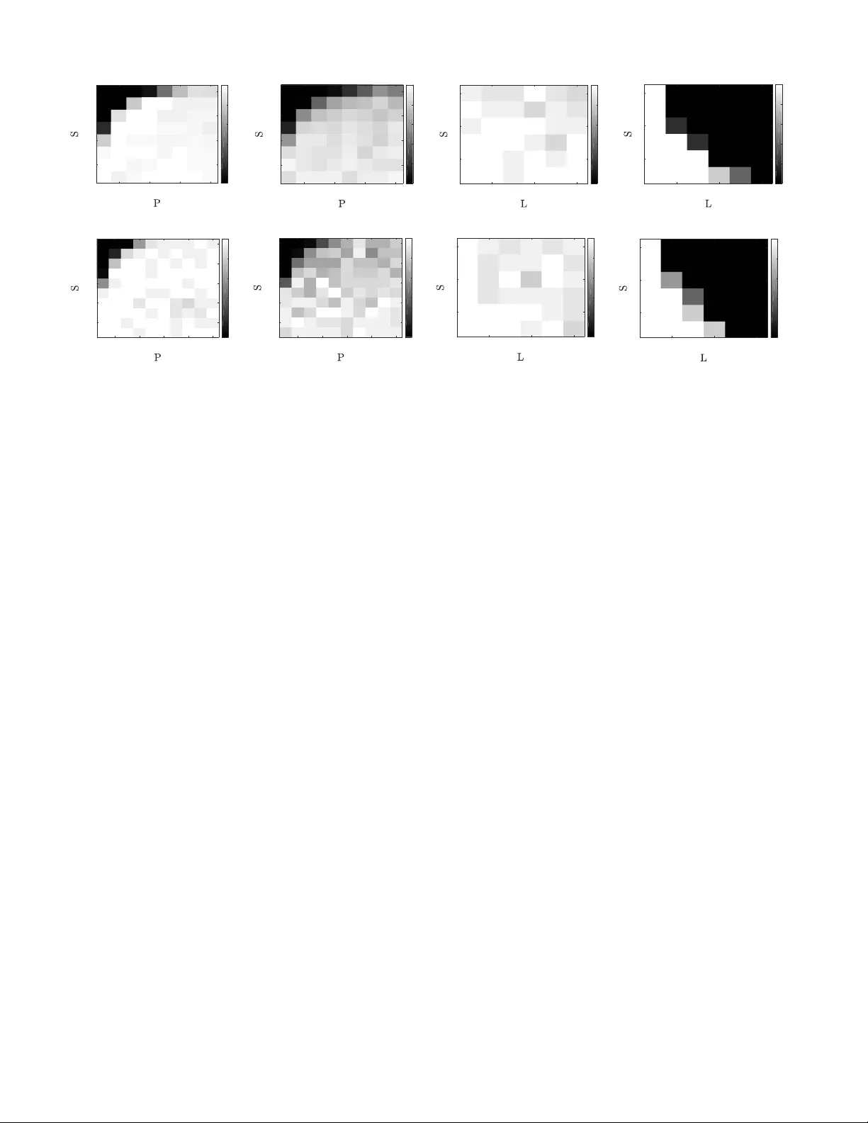
Blind Identification of In v ertible Graph Filters with Multiple Sparse Inputs Chang Y e, Rasoul Shafipour and Gonzalo Mateos Dept. of Electrical and Computer Engineering, Uni versity of Rochester , Rochester , NY , USA Abstract —This paper deals with problem of blind identification of a graph filter and its sparse input signal, thus broadening the scope of classical blind decon volution of temporal and spatial signals to irr egular graph domains. While the observations are bilinear functions of the unknowns, a mild r equirement on in vertibility of the filter enables an efficient conv ex formulation, without r elying on matrix lifting that can hinder applicability to large graphs. On top of scaling, it is argued that (non-cyclic) permutation ambiguities may arise with some particular graphs. Deterministic sufficient conditions under which the proposed con vex relaxation can exactly reco ver the unknowns are stated, along with those guaranteeing identifiability under the Bernoulli- Gaussian model for the inputs. Numerical tests with synthetic and real-world networks illustrate the merits of the proposed algorithm, as well as the benefits of leveraging multiple signals to aid the (blind) localization of sources of diffusion. Index T erms —Graph signal processing, network diffusion, bilinear equations, blind decon volution, con vex optimization. I . I N T R O D U C T I O N Network processes such as neural acti vities at dif ferent regions of the brain [9], [10], vehicle trajectories over road networks [4], or spatial temperature profiles measured by a wireless sensor network [19], can be represented as sig- nals supported on the nodes of a graph. Under the natural assumption that the signal properties are influenced by the graph topology (e.g., in a network diffusion or percolation process), the goal of graph signal processing (GSP) is to dev elop algorithms that exploit this relational structure. Ac- cordingly , generalizations of fundamental signal processing tasks ha ve been widely explored in recent work; see [14] for a comprehensi ve tutorial treatment. Notably graph filters – which generalize classical time-inv ariant systems – were con- ceiv ed as information-processing operators acting on graph- valued signals [18]. Mathematically , graph filters are linear transformations that can be expressed as polynomials of the so-termed graph-shift operator (Section II). The graph shift offers an alegbraic representation of network structure and can be viewed as a local diffusion operator . For the directed cycle graph representing e.g., periodic temporal signals, it boils down to the classical time-shift operator [18]. Gi ven a shift, the polynomial coef ficients fully determine the graph filter and are referred to as filter coefficients. Problem outline and en visioned applications. In this paper , we revisit the blind identification of graph filters with sparse inputs, with emphasis on modeling diffusion processes and W ork in this paper was supported by the NSF award CCF-1750428. Author emails: { cye7,rshafipo,gmateosb } @ur .rochester .edu. localization of the sources of diffusion [21]. Specifically , giv en observations of graph signals { y i } P i =1 that we model as out- puts of a diffusion filter (i.e., a polynomial in a known graph- shift operator), we seek to jointly identify the filter coefficients h and the input signals { x i } P i =1 that gav e rise to the network observations. This inv erse problem broadens the scope of classical blind deconv olution of temporal or spatial signals to graphs [1], [11]. Since the resulting bilinear inv erse problem is ill-posed, we assume that the inputs are sparse – a well- motiv ated setting when few seeding nodes inject a signal that is diffused throughout a network [21]. Accordingly , en visioned application domains include en vironmental monitoring (where are the heat or seismic sources?), opinion formation in social networks (who started the rumor?), neural signal processing (which brain regions were activ ated?), and epidemiology (who is patient zero for the disease outbreak?). Related work and contributions. Different from most ex- isting works dealing with source localization on graphs, e.g., [16], [24], like [15] the advocated GSP approach is applicable ev en when a single snapshot of the diffused signal is av ailable. Often the models of dif fusion are probabilistic in nature, and resulting maximum-likelihood source estimators can only be optimal for particular (e.g., tree) graphs [16], or rendered scal- able under restrictive dependency assumptions [5]. Relati ve to [9], [15], the proposed framework can accommodate signals defined on general undirected graphs and relies on a conv ex estimator of the sparse sources of diffusion. Furthermore, the setup where multiple output signals are observed (each one corresponding to a different sparse input), has not been thoroughly explored in con vex-relaxation approaches to blind decon volution of (non-graph) signals, e.g., [1], [13]; see [22] for a recent and inspiring alternati ve that we lev erage here. A note worthy approach was put forth in [21], which casts the (bilinear) blind graph-filter identification task as a linear in verse problem in the “lifted” rank-one, ro w-sparse matrix xh T . While the rank and sparsity minimization algorithms in [17], [21] can successfully recover sparse inputs along with low-order graph filters, reliance on matrix lifting can hinder applicability to lar ge graphs. Be yond this computational consideration, the overarching assumption of [21] is that the inputs { x i } P i =1 share a common support. Here instead we show how a mild requirement on in vertibility of the graph filter facilitates an efficient con ve x formulation for the multi-signal case with arbitrary supports (Section III); see also [22] for a time-domain precursor . In Section IV we take a closer look at inherent scaling and (non-cyclic) permutation ambiguities arising with some particular graphs. W e also briefly comment on identifiability under the Bernoulli-Gaussian model for the inputs [12], and state deterministic sufficient conditions under which the proposed con vex relaxation can exactly recover the unknowns. Numerical tests with synthetic graphs and a structural brain network corroborate the ef fectiveness of the proposed approach in recovering the sparse input signals (Section V). Concluding remarks are gi ven in Section VI. I I . P R E L I M I N A R I E S A N D P R O BL E M S TA T E M E N T Consider a weighted and undirected network graph G = ( V , A ) , where V is the set of vertices with cardinality |V | = N , and A ∈ R N × N is the symmetric graph adjacency matrix whose entry A ij denotes the edge weight between nodes i and j . As a more general algebraic descriptor of network structure, one can define a graph-shift oper ator S ∈ R N × N as any matrix ha ving the same sparsity pattern as G [18]. Accordingly , S can be viewed as a local diffusion (or av eraging) operator . Common choices are to set it to either A (and its normalized counterparts) or variations of adjacency and Laplacian matri- ces [6], [14]. Since S is real and symmetric, it is diagonalizable so that S = VΛV T , with Λ = diag ( λ 1 , . . . , λ N ) . Lastly , a graph signal x : V 7→ R N is an N -dimensional vector , where entry x i represents the signal value at node i ∈ V . A. Graph-filter models of network diffusion pr ocesses Let y be a graph signal supported on G , which is generated from an input graph signal x via linear network dynamics of the form y = α 0 Q ∞ l =1 ( I − α l S ) x = P ∞ l =0 β l S l x . (1) While S encodes only one-hop interactions, each successiv e application of the shift in (1) dif fuses x ov er G . Indeed, any process that can be understood as the linear propagation of a seed signal through a static graph can be written in the form in (1), and subsumes heat dif fusion, consensus and the classic DeGroot model of opinion dynamics as special cases [3]. The diffusion e xpressions in (1) are polynomials on S of possibly infinite degree, yet the Cayley-Hamilton theo- rem asserts they are equiv alent to polynomials of degree smaller than N . Upon defining the vector of coefficients h := [ h 0 , . . . , h L − 1 ] T and the shift-inv ariant graph filter H := h 0 I N + h 1 S + h 2 S 2 + . . . + h L − 1 S L − 1 = L − 1 X l =0 h l S l , (2) the signal model in (1) becomes y =  P L − 1 l =0 h l S l  x := Hx , for some particular h and L ≤ N . Due to the local structure of S , graph filters represent linear transformations that can be implemented in a distributed fashion [20], e.g., via L − 1 successiv e exchanges of information among neighbors. Lev eraging the spectral decomposition of S , graph filters and signals can be represented in the frequency domain. Specifically , let us use the eigen v alues of S to define the N × L V andermonde matrix Ψ L , where Ψ ij := λ j − 1 i . The frequency representations of a signal x and filter h are defined as ˜ x := V T x and ˜ h := Ψ L h , respectively . The latter follows since the output y = Hx in the frequency domain is given by ˜ y = diag  Ψ L h  V T x = diag  ˜ h  ˜ x = ˜ h ◦ ˜ x . (3) This identity can be seen as a counterpart of the con volution theorem for temporal signals, where ˜ y is the elementwise product ( ◦ ) of ˜ x and the filter’ s frequenc y response ˜ h := Ψ L h . B. Pr oblem formulation For gi ven shift operator S and filter order L , suppose we observe P output signals collected in a matrix Y = [ y 1 , . . . , y P ] ∈ R N × P such that Y = HX , where X = [ x 1 , . . . , x P ] ∈ R N × P is sparse having at most S  N non-zero entries per column. The goal is to perform blind identification of the graph filter (and its input signals), which amounts to estimating sparse X and the filter coef ficients h up to scaling and (possibly) permutation ambiguities; see Section IV. Sparsity is well moti vated when the signals in Y represent diffused versions of a few localized sources in G , here indexed by supp ( X ) := { ( i, j ) | X ij 6 = 0 } . Moreover , the non-sparse formulation is ill-posed, since the number of unknowns N P + L in { X , h } exceeds the N P observations in Y . All in all, using (3) the diffused source localization task can be stated as a feasibility problem of the form find { X , h } s. to Y = V diag  Ψ L h  V T X , k X k 0 ≤ P S, (4) where the ` 0 -(pseudo) norm k X k 0 := | supp ( X ) | counts the non-zero entries in X . In words, the goal is to find the solution to a system of bilinear equations subject to a sparsity constraint in X ; a hard problem due to the non-con ve x ` 0 -norm as well as the bilinear constraints. T o deal with the latter, building on [22] we will henceforth assume that the filter H is in vertible. I I I . C O N V E X R E L A X A T I O N F O R I N V E RT I B L E F I LT ER S Here we show how to efficiently tackle the blind graph filter identification problem, through a con ve x relaxation of (4) when the diffusion filter is in vertible. T o that end, note from (3) that graph filter H is in vertible if and only if ˜ h i = P L − 1 l =0 h l λ l i 6 = 0 , for all i = 1 , . . . , N . In words, the frequency response of the filter should not vanish at the graph frequencies { λ i } . In such case one can show that the inv erse operator G := H − 1 is also a graph filter on G , which can be uniquely represented as a polynomial in the shift S of degree at most N − 1 [18, Theorem 4]. T o be more specific, let g ∈ R N be the vector of inv erse-filter coefficients, i.e., G = P N − 1 l =0 g l S l . Then one can equiv alently rewrite the generativ e model Y = HX for the observations as X = GY = V diag ( ˜ g ) V T Y , (5) where ˜ g := Ψ N g ∈ R N is the in verse filter’ s frequency response and Ψ N ∈ R N × N is V andermonde. Naturally , G = H − 1 implies the condition ˜ g ◦ ˜ h = 1 N on the frequency responses, where 1 N denotes the N × 1 vector of all ones. Lev eraging (5), one can recast (4) as a linear in verse problem min { X , ˜ g } k X k 0 , s. to X = V diag ( ˜ g ) V T Y , X 6 = 0 . (6) This approach is markedly different from the matrix lifting technique used in [21] to handle the bilinear equations in (4). The ` 0 norm in (6) makes the problem NP-hard to optimize. Over the last decade or so, con ve x-relaxation approaches to Algorithm 1 Iterativ ely-reweighted ` 1 minimization for (7) 1: Input: Matrix Y T V  V , δ > 0 and  > 0 . 2: Initialize t = 0 , w (0) = 1 N P and X (0) = 0 . 3: repeat 4: Solve ˜ g ( t +1) = argmin ˜ g    w ( t ) ◦  ( Y T V  V ) ˜ g     1 s. to 1 T N ˜ g = 1 . 5: Form X ( t +1) = ( Y T V  V ) ˜ g ( t +1) . 6: Update w ( t +1) i = 1 [ vec ( X ( t +1) )] i + δ , i = 1 , 2 , ..., N P . 7: t ← t + 1 . 8: until k X ( t +1) − X ( t ) k 1 / k X ( t ) k 1 ≤  9: retur n ˆ ˜ g := ˜ g ( t +1) and ˆ X := X ( t +1) tackle sparsity minimization problems hav e enjoyed remark- able success, since they often entail no loss of optimality . Accordingly , we instead: (i) seek to minimize the ` 1 -norm con vex surrogate of the cardinality function, that is k X k 1 = P i,j | X ij | ; and (ii) express the filter in the graph spectral domain as in (5) to obtain the cost k X k 1 = k GY k 1 = k V diag ( ˜ g ) V T Y k 1 = k ( Y T V  V ) ˜ g k 1 , where  denotes the Khatri-Rao (i.e., columnwise Kronecker) product. This suggests solving the con vex ` 1 -synthesis prob- lem (in this case a linear program), e.g., [23], namely b ˜ g = argmin ˜ g ∈ R N k ( Y T V  V ) ˜ g k 1 , s. to 1 T N ˜ g = 1 . (7) While the linear constraint in (7) av oids b ˜ g = 0 , it also serves to fix the scale of the solution. As a result, under the pragmatic assumption that the dif fu- sion filter is inv ertible, one can readily use e.g., an of f-the-shelf interior-point method or a specialized sparsity-minimization algorithm to solve (7) efficiently . Different from the solvers in [17], [21], the aforementioned algorithmic alternatives are free of expensi ve singular-v alue decompositions per iteration. W e have found that overall performance can be improved via the iteratively-re weighted ` 1 -norm minimization procedure tabulated under Algorithm 1; see also [2] for a justification of such refinement. In any case, notice that once the frequency response b ˜ g of the inv erse filter is recovered, one can readily reconstruct the sources via ˆ X = ( Y T V  V ) ˜ g as well as the filter H , if desired. In the next section we will take a closer look at the inherent ambiguities associated with the bilinear model Y = HX , some of which are unique to the network setting dealt with here. These are of course important to delineate the scope of identifiability (i.e., uniqueness) results. W e will complete our discussion with deterministic suf ficient conditions under which the conv ex relaxation (7) is tight. I V . I D E N T I FI A B I L I T Y A N D E X A C T R E C OV E RY T o establish further connections with blind decon volution of periodic discrete-time signals, recall these can be viewed as graph signals supported on the directed cycle graph (whose Fig. 1. T oy undirected graph (left) used to illustrate the symmetric permutation ambiguity between nodes 2 and 4 . The fourth eigenvector v 4 of S = A (center) has the problematic form. Then if { X 0 , ˜ h 0 } satisfies the bilinear equations Y = V diag ( ˜ h ) V T X , so does { PX 0 , diag ( p ) ˜ h 0 } for the sho wn permutation matrix P (right) and p = [1 , 1 , 1 , − 1 , 1 , 1 , 1] T . circulant adjacency matrix is diagonalized by the DFT ba- sis) [18]. In this special case, the blind identification task is known to suffer from unav oidable scaling and circulant-shift ambiguities; see e.g., [1], [22]. Here we examine more general symmetric permutation ambiguities arising with unweighted graphs, and briefly outline a relev ant identifiability result as well as preliminary exact recovery conditions for (7). A. P ermutation ambiguities for some unweighted graphs In solving the bilinear in verse problem formulated in Sec- tion II, for some particular graphs in addition to scaling we may also encounter (non-cyclic shift) permutation ambiguities. W e can resolve the scaling ambiguity by e.g., a fortiori setting k ˜ g 0 k 1 = 1 as in the experiments of Section V, where ˜ g 0 is the ground-truth frequency response of the inv erse filter . Inspired by the identifiability studies for sparsity-constrained bilinear problems [12], here we examine said permutation ambiguities for unweighted graphs with shift S = VΛV T . Let { X 0 , ˜ h 0 } collect the ground-truth sparse input signals and the filter’ s frequency response, respectiv ely . Let u ( i,j ) ∈ R N be a unit-norm vector with zero entries except for u ( i,j ) i = − u ( i,j ) j = 1 / √ 2 . As we sho w next, a permutation ambiguity arises if, say , the k th eigen vector of S (i.e., the k th column of V ) has the form u ( i,j ) . Indeed, in that case one could introduce a binary signed vector p ∈ {− 1 , 1 } N with a single neg ativ e entry p k = − 1 , to construct another solution of the form X 1 := PX 0 , ˜ h 1 := diag ( p ) ˜ h 0 , (8) where P = I N − 2 u ( i,j ) ( u ( i,j ) ) T = V diag ( p ) V T is a symmetric permutation matrix that interchanges the signal values at nodes i ( x i ) and j ( x j ) when applied to the graph signal x . It is immediate that the pair in (8) satisfies the generativ e model Y = HX = V diag ( ˜ h ) V T X . So, if u ( i,j ) is an eigen vector of S then we can not distinguish the values at nodes i and j and the problem remains non-identifiable. T o ex emplify this situation, consider the toy graph illustrated in Fig 1-(left). One can consider the adjacency matrix as the shift ( S = A ) and denote the corresponding eigen vectors as V = [ v 1 , · · · , v 7 ] . Fig 1-(center) sho ws that v 4 = u (2 , 4) . Then it follows that for the matrix P in Fig 1-(right) and the vector p = [1 , 1 , 1 , − 1 , 1 , 1 , 1] T , one can construct another solution { X 1 , ˜ h 1 } 6 = { X 0 , ˜ h 0 } using (8). In other words, nodes 2 and 4 are indistinguishable. While it is challenging to obtain a formal characterization of problematic graphs, in practice we hav e encountered issues with dense networks as well as with some very sparse graphs. For (continuous-valued) weighted graphs such ambiguities effecti vely disappear . Before moving on to issues of exact recov ery , a remark on identifiability of (4) for a simple but widely adopted (random) sparsity model is in order . Remark 1 (Identifiability f or Bernoulli-Gaussian model) Because of its analytical tractability , the Bernoulli-Gaussian model is widely adopted to describe and generate random sparse matrices such as X ∈ R N × P (we also use it for the simulations in Section V). Sparse matrices adhering to the model are X = Ω ◦ R , where Ω ∈ R N × P is an i.i.d. Bernoulli matrix with parameter θ (i.e., P [Ω ij = 1] = θ ), and R ∈ R N × P is an independent random matrix with i.i.d. symmetric random variables drawn from a standard Gaussian distrib ution. Under the Bernoulli-Gaussian model, [12, Proposition 40] asserts that problem (6) is identifiable (up to scaling and symmetric permutation ambiguities) with probability at least 1 − exp ( − cθ P ) , for 1 N < θ < 1 4 and P > cN log ( N ) , where c > 0 is a sufficiently large constant. B. Exact r ecovery conditions Suppose that (6) is identifiable and let { X 0 , ˜ g 0 } be the solution. The following proposition (that relies heavily on [23, Theorem 1]) offers sufficient conditions under which the con vex relaxation (7) succeeds in e xactly recov ering { X 0 , ˜ g 0 } . Proposition 1 Let I := supp ( vec ( X 0 )) index the non-zero entries of vectorized X 0 , and let I c be the complement of I . Moreov er , define Z := Y T V  V ∈ R N P × N and let Z S be the submatrix of Z with rows index ed by S ⊂ { 1 , 2 , ..., N P } . Then, the solution to (7) is unique and equal to ˜ g 0 if the two following conditions are satisfied: C1) rank ( Z I c ) = N − 1 ; and C2) There exists a vector f ∈ R N P such that Z T f = γ 1 N for some γ 6 = 0 , such that f I = sign ( Z I ˜ g 0 ) and k f I c k ∞ < 1 . Proof : As per [23, Theorem 1], ˜ g 0 is the unique solution of (7) if ker ( Z I c ) ∩ ker ( 1 N ) = { 0 } . But since ˜ g 0 ∈ ker ( Z I c ) and ˜ g 0 6∈ ker ( 1 N ) because of the constraint in (7), then C1) ensures said intersection is { 0 } . Optimality condition C2) essentially requires 1 N to belong to the set of subgradients of k Z ˜ g k 1 at ˜ g 0 ; see [23, Theorem 1] for further details.  Naturally , a more insightful exact recov ery and sample complexity result along the lines of the one in Remark 1 would be most v aluable [i.e., when are C1)-C2) satisfied for the Bernoulli-Gaussian model?], but left as future work. V . N U M E R I C A L R E S U LT S W e assess the performance of our proposed approach by testing the iteratively-re weighted ` 1 -norm minimization pro- cedure in Algorithm 1. The per-iteration sparse recov ery problems are solved using CVX [7]. Simulation setup. In all cases we consider undirected graphs with graph-shift operator chosen as the normalized adjacency matrix S = D − 1 2 AD − 1 2 , where D := diag ( A1 N ) is a diagonal matrix of node degrees. The ground-truth sparse input matrix X 0 is drawn from a Bernoulli-Gaussian model as in Remark 1, for varying parameters N , P , and sparsity lev el (i.e., number of nonzero entries) S . Filter coefficients h 0 are generated according to h 0 = ( e 1 + α b ) / k e 1 + α b k 1 , where e 1 = [1 , 0 , · · · , 0] T ∈ R L is the first canonical basis vector and entries of b ∈ R L are drawn independently from a standard Gaussian distribution. Such a model for h 0 is inspired by [22], and we later corroborate that the recov ery performance improv es as α decreases. Also note that h 0 is normalized to unit ` 1 -norm to fix the scale of the problem. Finally , giv en X 0 and H 0 = V diag ( Ψ L h 0 ) V T , the N × P matrix of observations is generated as Y = H 0 X 0 . The relative recov ery error e X = k ˆ X − X 0 k / k X 0 k is adopted as figure of merit to ev aluate algorithmic performance. W e estimate the rate of successful recovery for synthetic and real-world graphs under dif ferent parameters by defining a successful recovery as one with e X < 0 . 01 . Random graphs. Consider Erd ˝ os-R ´ enyi random graphs with N = 50 nodes, where edges are formed independently with probability p = 0 . 3 . The rate of successful recovery is estimated for realizations of random graphs which are connected and do not giv e rise to permutation ambiguities (cf. Section IV -A). Figures 2(a) and 2(b) depict the recovery rates as a function of P and S for α = 0 . 1 and 0 . 3 , respectiv ely , av eraged over 100 realizations for (in vertible) graph filters of order L = 5 . As expected, in both cases reco very is more challenging for larger S and smaller P ; see the dark-gray area of low-success probability around the top-left corner . More- ov er , decreasing α makes successful recov ery more likely . For instance, for α = 0 . 1 [Fig. 2(a)] we can successfully recov er dense input signals with e.g., S ≈ N/ 2 = 25 and only P = 10 observations. For (effecti vely) lower -order filters resulting in more localized diffusion dynamics, one obtains fa vorable recovery performance. W e also compare the proposed approach against its less- scalable, matrix lifting-based precursor in [21]. Figures 2(c) and 2(d) respectiv ely show the recov ery rates for both methods as a function of sparsity S and filter order L , for N = 50 , p = 0 . 3 , P = 10 , and α = 0 . 5 av eraged over 20 realiza- tions. Apparently , Algorithm 1 [Fig. 2(c)] can be successful ov er a larger range of values of L . Moreov er , it uniformly outperforms the algorithm in [21, Problem (9)]; see Fig. 2(d). Brain graph. W e also consider a structural brain graph with N = 66 nodes or neural regions of interest (R OIs), and edge weights giv en by the density of anatomical connections between regions [8]. The lev el of activity of each R OI can be represented by a graph signal x , thus successive applications of S model a linear e volution of the brain activity pattern. Supposing we observe a linear combination (filter) of the ev olving states of an originally sparse brain signal, then blind identification amounts to jointly estimating which regions were originally active, the acti vity in these re gions and the coefficients of the linear combination. W e repeat the recovery-rate analysis performed for Erd ˝ os- R ´ enyi graphs averaged o ver 20 realizations, and report the results in Figs. 2(e)–(h). Figures 2(e) and 2(f) showcase that our algorithm successfully identifies the initial excitation regions as well as the diffusion coefficients over a broad region in parameter space. By comparing Figs. 2(g) and 2(h), 10 20 30 40 10 20 30 40 0 0.2 0.4 0.6 0.8 1 (a) 10 20 30 40 10 20 30 40 0 0.2 0.4 0.6 0.8 1 (b) 2 4 6 2 4 6 0 0.2 0.4 0.6 0.8 1 (c) 2 4 6 2 4 6 0 0.2 0.4 0.6 0.8 1 (d) 10 20 30 40 50 10 20 30 40 50 0 0.2 0.4 0.6 0.8 1 (e) 10 20 30 40 50 10 20 30 40 50 0 0.2 0.4 0.6 0.8 1 (f) 2 4 6 2 4 6 0 0.2 0.4 0.6 0.8 1 (g) 2 4 6 2 4 6 0 0.2 0.4 0.6 0.8 1 (h) Fig. 2. Rate of recovery of X as a function of S (number non-zero entries in X ) and P (number of observations) in N = 50 -node Erd ˝ os-R ´ enyi graphs with p = 0 . 3 (edge existence probability) for (a) α = 0 . 1 and (b) α = 0 . 3 , using Algorithm 1. Plots (e) and (f) are counterparts of (a) and (b), respectiv ely , for the structural brain network in [8]. Recovery rate in Erd ˝ os-R ´ enyi graphs ( N = 50 , p = 0 . 3 ) as a function of S and L (filter order) using (c) Algorithm 1 and (d) the matrix-lifting approach of [21]. Plots (g) and (h) are counterparts of (c) and (d), respectively , for the aforementioned structural brain network. it is apparent that also in this setting the proposed approach outperforms the state-of-the-art method in [21], corroborating the effecti veness of Algorithm 1. V I . C O N C L U S I O N W e studied the problem of blind graph filter identification, which extends blind decon volution of time (or spatial) domain signals to graphs. By introducing a mild assumption on in vertibility of the graph filter , we obtained a computationally simpler conv ex relaxation for (diffused) source localization in the multi-signal case. Ongoing work includes deriving suitable graph-dependent conditions under which exact (and stable) recov ery can be guaranteed, even when only a fraction of nodes is observed. This is a challenging problem, since the fa vorable (circulant) structure of time-domain filters is no longer present in the network-centric setting dealt with here. R E F E R E N C E S [1] A. Ahmed, B. Recht, and J. Romberg, “Blind deconv olution using con vex programming, ” IEEE T rans. Inf. Theory , vol. 60, no. 3, pp. 1711– 1732, 2014. [2] E. J. Candes, M. B. W akin, and S. P . Boyd, “Enhancing sparsity by reweighted ` 1 minimization, ” Journal of F ourier Analysis and Applica- tions , vol. 14, no. 5-6, pp. 877–905, 2008. [3] M. H. DeGroot, “Reaching a consensus, ” Journal of the American Statistical Association , vol. 69, pp. 118–121, 1974. [4] J. A. Deri and J. M. F . Moura, “Ne w York City taxi analysis with graph signal processing, ” in Pr oc. IEEE Global Conf. on Signal and Information Pr ocess. , Dec. 2016, pp. 1275–1279. [5] S. Feizi, M. M ´ edard, G. Quon, M. Kellis, and K. Duffy , “Network infusion to infer information sources in networks, ” arXiv preprint arXiv:1606.07383 [cs.SI] , 2016. [6] A. Gavili and X.-P . Zhang, “On the shift operator, graph frequency , and optimal filtering in graph signal processing, ” IEEE T rans. Signal Pr ocess. , vol. 65, no. 23, pp. 6303–6318, 2017. [7] M. Grant and S. Boyd, “CVX: Matlab software for disciplined conv ex programming, version 2.1, ” http://cvxr.com/cvx, Mar . 2014. [8] P . Hagmann, L. Cammoun, X. Gigandet, R. Meuli, C. J. Honey , V . J. W edeen, and O. Sporns, “Mapping the structural core of human cerebral cortex, ” PLoS Biology , vol. 6, no. 7, p. e159, 2008. [9] C. Hu, X. Hua, J. Ying, P . M. Thompson, G. E. Fakhri, and Q. Li, “Localizing sources of brain disease progression with network dif fusion model, ” IEEE J. Sel. T opics Signal Pr ocess. , vol. 10, no. 7, pp. 1214– 1225, 2016. [10] W . Huang, L. Goldsberry , N. F . W ymbs, S. T . Grafton, D. S. Bassett, and A. Ribeiro, “Graph frequency analysis of brain signals, ” IEEE J. Sel. T opics Signal Process. , vol. 10, no. 7, pp. 1189–1203, Oct. 2016. [11] A. Levin, Y . W eiss, F . Durand, and W . T . Freeman, “Understanding blind decon volution algorithms, ” IEEE T rans. P attern Anal. Mach. Intell. , vol. 33, no. 12, pp. 2354–2367, 2011. [12] Y . Li, K. Lee, and Y . Bresler , “Identifiability in bilinear inv erse problems with applications to subspace or sparsity-constrained blind gain and phase calibration, ” IEEE T rans. Inf. Theory , vol. 63, no. 2, pp. 822– 842, Feb 2017. [13] S. Ling and T . Strohmer , “Self-calibration and biconv ex compressiv e sensing, ” Inverse Pr oblems , vol. 31, no. 11, p. 115002, 2015. [14] A. Ortega, P . Frossard, J. Kov a ˘ cevi ´ c, J. M. F . Moura, and P . V an- derghe ynst, “Graph signal processing, ” arXiv preprint [eess.SP] , 2017. [15] R. Pena, X. Bresson, and P . V andergheynst, “Source localization on graphs via ` 1 recovery and spectral graph theory , ” in Pr oc. IEEE Image, V ideo, and Multidimensional Signal Process. W orkshop , 2016, pp. 1–5. [16] P . C. Pinto, P . Thiran, and M. V etterli, “Locating the source of diffusion in large-scale networks, ” Physical Review Letters , vol. 109, no. 6, p. 068702, 2012. [17] D. Ram ´ ırez, A. G. Marques, and S. Segarra, “Graph-signal reconstruc- tion and blind decon volution for diffused sparse inputs, ” in Proc. Int. Conf. Acoustics, Speech, Signal Process. , Mar . 2017, pp. 4104–4108. [18] A. Sandryhaila and J. M. Moura, “Discrete signal processing on graphs, ” IEEE T rans. Signal Pr ocess. , vol. 61, no. 7, pp. 1644–1656, 2013. [19] I. D. Schizas, G. Mateos, and G. B. Giannakis, “Distributed LMS for consensus-based in-network adaptive processing, ” IEEE T rans. Signal Pr ocess. , vol. 57, no. 6, pp. 2365–2381, Mar. 2009. [20] S. Segarra, A. G. Marques, and A. Ribeiro, “Optimal graph-filter design and applications to distributed linear network operators, ” IEEE T rans. Signal Pr ocess. , vol. 65, no. 15, pp. 4117–4131, Aug 2017. [21] S. Segarra, G. Mateos, A. G. Marques, and A. Ribeiro, “Blind identifi- cation of graph filters, ” IEEE T rans. Signal Pr ocess. , vol. 65, no. 5, pp. 1146–1159, Mar . 2017. [22] L. W ang and Y . Chi, “Blind decon volution from multiple sparse inputs, ” IEEE Signal Process. Lett. , vol. 23, no. 10, pp. 1384–1388, 2016. [23] H. Zhang, M. Y an, and W . Y in, “One condition for solution uniqueness and robustness of both l1-synthesis and l1-analysis minimizations, ” Adv . Comput. Math. , vol. 42, no. 6, pp. 1381–1399, 2016. [24] P . Zhang, J. He, G. Long, G. Huang, and C. Zhang, “T owards anomalous diffusion sources detection in a large network, ” A CM T . Internet T echn. , vol. 16, no. 1, p. 2, 2016.