Multisensor Data Fusion for Water Quality Monitoring using Wireless Sensor Networks

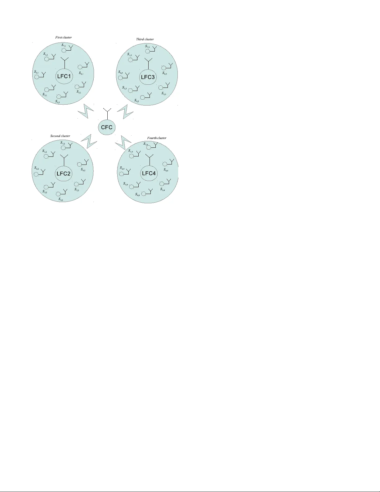
Multisensor Data Fusion for W ater Quality Monitoring using W ireless Sensor Networks Ebrahim Karami, Francis M. Bui, and Ha H. Nguyen Department of Electrical and Computer Engineering, Univ ersity of Saskatchew an, Canada email: { ebk855,francis.bui,ha.nguyen } @mun.ca Abstract —In this paper , the application of hierarchical wireless sensor networks in water quality monitoring is in vestigated. Adopting a hierarchical structure, the set of sensors is divided into multiple clusters where the value of the sensing parameter is almost constant in each cluster . The members of each cluster transmit their sensing information to the local fusion center (LFC) of their corresponding cluster , wher e using some fusion rule, the recei ved information is combined, and then possibly sent to a higher -level central fusion center (CFC). A two- phase processing scheme is also en visioned, in which the first phase is dedicated to detection in the LFC, and the second phase is dedicated to estimation in both the LFC and the CFC. The f ocus of the present paper is on the problem of decision fusion at the LFC: we propose hard- and soft-decision maximum a posteriori (MAP) algorithms, which exhibit flexibility in minimizing the total cost imposed by incorrect detections in the first phase. The pr oposed algorithms are simulated and compared with con ventional fusion techniques. It is shown that the proposed techniques r esult in lower cost. Furthermore, when the number of sensors or the amount of contamination increases, the performance gap between the proposed algorithms and the existing methods also widens. Index T erms —W ater quality , monitoring, contamination warn- ing systems, wireless sensor networks, data fusion, distributed detection, maximum a posteriori algorithms. I . I N T RO D U C T I O N Providing a reliable supply of potable water is an important goal in todays society . T o this end, water contamination warning systems (WCWSs) are typically deployed to monitor the quality of water . At the same time, wireless sensor networks (WSNs) hav e found extensi ve applications in monitoring physical or environmental conditions such as temperature, sound, pressure, etc. Therefore in this context, WCWSs hav e been one of the most recent embodiments of WSNs [1]–[4]. In a WCWS, the type of the parameters that must be monitored and controlled depends on the use of water . For example, for drinking water , chemical contamination is much more important to monitor; while for industrial applications, physical contaminations are more important, because physical objects in the water may damage industrial equipments that work with water [5]. Therefore, when used This work was supported by an NSERC engage grant and IBM Canada. in isolation, a particular sensor may produce large sensing errors, responsible for incorrect or missing alarms. On the other hand, reliable and high-quality sensors, with lo wer variance in the sensing error , are in variably more expensiv e. As such, in a WCWS where many sensors may be needed to provide sufficient coverage of large geographical areas, e.g., a riv er or a water distribution system, the total cost may prov e economically infeasible. In addition, for a WSN, sensing error is not the only source of error: the quality of the wireless links is another major limiting factor . Therefore, to combat both sources of error , collaboration among the sensors in the network is useful in enabling distributed parameter estimation (DPE) [3]. In DPE, each sensor is allowed to either send its measurement to a fusion center , or share it with other sensors which are in its transmission range [6]. The hierarchical structure increases the efficiency of the WSN in many aspects. In a hierarchical structure, the monitoring area is divided into multiple clusters where the value of the sensing parameter is almost constant inside each cluster b ut it may v ary from one cluster to another . In general, the cross correlation between the values of the parameter in two clusters depends on some factors such as relati ve distance between the clusters, direction and velocity of the water flow . As shown in Fig. 1, each cluster has a local fusion center (LFC) which makes a local decision and then sends it to a central fusion center (CFC) to make the final decision. When a WSN is used to monitor the water quality , the sensing information from different types of sensors such as pH, DO (dissolved Oxygen), arsenic, permanganate and so on, are sensed and transmitted to the LFC [3]. Using the hierarchical structure not only reduces the required power for communication between sensors and consequently increases the lifetime of the batteries, but also reduces the complexity of routing and scheduling in the wireless network. The cluster size can be optimized to minimize the required communications overhead among sensors [7]. T o increase the bandwidth efficiency in a DPE based system, one can perform monitoring in two phases. In the first phase, the quality of the water is constantly monitored by sensors and each sensor periodically sends a binary signal to the LFC where 1 means that the water has become contaminated, and 0 means the water is healthy . Then the LFC combines the receiv ed binary signals using some fusion rule and if its final decision is whether the water in that area is contaminated, the system goes to the second phase where the LFC dedicates a much larger bandwidth to its members and asks them to send the values of the monitoring parameters for more exact processing and forwarding them to the CFC. This two-stage approach reduces the required bandwidth because the system mostly works in the first phase where only low-rate binary decisions are transmitted from sensors to the LFC and this communication needs much less bandwidth compared to the case where the measured signal is directly sent to LFC. This paper focuses on the local detection in the LFC, i.e., phase 1, while deferring phase 2 to a future work. The objectiv e is to formulate an optimum detection for each LFC. Conv entional fusion techniques for binary decisions are OR-rule, AND-rule, and n -out-of- M -rule. For the simpler OR-rule and AND-rule, the recei ved binary decisions from the sensors are simply fed into a logical OR or AND operator to make the final decision. Howe ver , with a more general n -out-of- M -rule, the final decision is a logical true, i.e., bit 1, if at least n out of M sensors have triggered alarm. Obviously the AND-rule results in a high rate of missed detections, making it unsuitable in WCWS where any contamination misdetection might be dangerous. On the other hand, the OR-rule leads to a high false alarm rate, so that the system may operate mostly in the second phase, where bandwidth and the other network resources are wasted. The n -out-of- M -rule offers a more flexible compromise, where the trade-off between missed detection and false alarm rates may be more properly balanced, based on a particular application scenario. In applying fusion rules, a consideration that warrants attention is the utilization of sensor statistics. While con ventional fusion techniques, including n -out-of- M -rule, do not utilize the sensor statistics directly , it is e vident that a detection rule needs to exploit the a vailable statistical information in order to achie ve optimality , especially when applied in a real implementation. T o a certain extent, more recent w orks take into account the sensor statistics in optimizing the parameter n [8], [9]. Nevertheless, the fact that the sensors may have dif ferent accuracy is not directly accounted for in this optimization. Furthermore, giv en that the parameter statistics may vary in a realistic situation, the value of n would have to be accordingly adapted for optimality . Other more statistically deriven fusion methods include the maximum likelihood (ML) and maximum a posteriori (MAP) algorithms. The ML detection minimizes the sum of false alarm and missed detection rates; as such, it outperforms the optimized n -out-of- M -rule [10]. Similarly , the MAP algorithm minimizes the total probability of error . Howe ver , it should be noted that, for practical water monitoring applications, the probability of missed detection is typically more important than the probability of false alarma fact ignored by both the con ventional ML and MAP algorithms. In light of the abov e limitations of con ventional data fusion in the context of water monitoring, this paper proposes a flexible MAP detector that is nonetheless of low complexity which minimizes the total cost imposed by false alarms and missed detections. In other words, by appropriately weighting these probabilities, a higher priority can be assigned to either quantity , to suit a particular application scenario; the proposed MAP detector then minimizes this weighted error rate. The rest of this paper is organized as follo ws. The system model and problem definition are presented in Sec. II. Fusion techniques based on the MAP algorithm, and their modifica- tions are presented in Sec. III. Lastly , simulation results are presented in Sec. IV , with the conclusion in the Sec. V . I I . S Y S T E M M O D E L A N D P R O B L E M D E FI N I T I O N Consider a network with N total sensors, used to monitor the quality of water in a measurement area, e.g., a pool or a riv er . As discussed in the abov e, this area is hierarchically divided into multiple clusters, as illustrated in Fig. 1. Howe ver , since the present paper addresses phase 1 of the processing scheme, i.e., fusion in the LFC, the focus is on a single cluster , with M active sensors. Let θ denote the parameter to be measured, which, by cluster selection, should be nearly constant at all M sensors in the cluster . As noted previously , depending on the application, θ may represent quantities such as PH, DO, arsenic concentration, etc. Therefore, θ is generally a (bounded) continuous-valued quantity . Next, let e m be the sensing error at the m th sensor . Then, the measured parameter can be modeled as ˆ θ m = g ( θ, e m ) , (1) where g ( . ) is a generalized function representing the sensor characteristic. With small errors in the sensor dynamic range, linear approximation provides the simplification ˆ θ m = α m θ + e m , (2) where α m = 1 if the sensors are properly calibrated. The measured signal ˆ θ m is compared with τ max and τ min to decide whether to send decision signal x m = 0 or 1 to the LFC. In other words, if the measured pH is outside the safety range then a bit 1 is modulated and sent to the LFC, otherwise bit 0 is modulated and sent. In the next step, decisions made by the members of the cluster are transmitted to the LFC through orthogonal channels. Since the transmitted signal is very narro w band, we can assume flat fading channel model. Assuming h m as the Rayleigh flat fading channel for the link between m th sensor and the LFC, n m as its corresponding additiv e complex Gaussian noise with variance σ 2 n , and binary Fig. 1. Distributed parameter estimation using a hierarchical WSN. phased shift keying modulation (BPSK) scheme, the recei ved complex signal r m at the LFC is r m = h m (1 − 2 x m ) + n m . (3) The optimum fusion method is defined as finding the most probable estimation of x , for giv en set of observations r m s where x = 0 means water is safe and x = 1 means water is contaminated. An optimum fusion rule can be defined for either soft detector or hard detector i.e., where ˆ x m s as hard estimations of the x m s are used. For the m th sensor, based on the precision of the sensor , two new parameters, P m F as the probability of the false alarm and P m M as the probability of missed detection, are defined at sensor lev el. P m F means the probability that the measuring parameter is inside its allowed range but the sensor detects it as outside the range. Like wise, P M means the probability that, the measuring parameter is outside its allowed range i.e. water is contaminated but the sensor does not detect the contamination. Probability of false alarm and missed detection for pH sensors are calculated from equations (26) and (27) and using following equations, P m F = P ( x m = 1 | x = 0) . (4) P m M = P ( x m = 0 | x = 1) . (5) W ith the distribution of the sensing parameter and sensing error and using (2), (4), and(5), P m F and P m M can be easily calculated. Since the wireless channel is noisy , the transmitted informa- tion is detected with some error . One can define the equiv alent probabilities of missed detection and false alarm for each sensor as follows, ˜ P m F = P m F (1 − P m b ) + (1 − P m F ) P m b . (6) ˜ P m M = P m M (1 − P m b ) + (1 − P m M ) P m b . (7) where ˜ P m F and ˜ P m M are the equiv alent probabilities of false alarm and missed detection for the m th sensor respectively and P m b is the bit error rate for signal receiv ed from the m th sensor , which depends on the quality of the channel from the sensor to the LFC. P m F and P m M are considered as two basic criteria to compare the performance of the sensing techniques at either the sensor lev el or the LFC level, i.e., for the final decision x tot made by the LFC. In this case, we call them total probabilities of false alarm P tot F and total probability of missed detection P tot M defined as follow , P tot F = P  x tot = 1 | x = 0  , (8) P tot M = P ( x tot = 0 | x = 1) . (9) The total probability of error , P tot E , is calculated as follows: P tot E = P  x tot = 1 , x = 0  + P  x tot = 0 , x = 1  . (10) By substituting (8) and (9) in (10) , we hav e P tot E = P H 1 P tot M + P H 0 P tot F , (11) where P H 0 = P ( x = 0) and P H 1 = P ( x = 1) . I I I . M A P F U S I O N T E C H N I Q U E This section presents both hard detection (HD) and soft detection (SD) based MAP fusion rules. A. SD MAP Fusion Algorithm The SD MAP fusion algorithm is defined as x S D − M AP = arg max x P ( x | r 1 , r 2 , ..., r M − 1 , r M ) . (12) (12) is con ventionally solved by likelihood ratio (LR) test [11]. Therefore likelihood ratio ζ S D is defined as follows, ζ S D = P ( x tot = 1) P ( x tot = 0) , (13) and using Bayes’ rule, (13) is expanded as ζ S D = M Y m =1 P ( r m | x = 1) P ( r m | x = 0) P ( x = 1) P ( x = 0) , (14) and then using (3), (14) is calculated by (15) and from (3), (4), and (5) ζ S D is calculated by (16) Consequently if ζ S D > 1 then x S D − M AP = 1 and otherwise x S D − M AP = 0 . B. HD MAP Fusion Algorithm The HD MAP fusion algorithm is defined as x H D = arg max x P ( x | ˆ x 1 , ˆ x 2 , ..., ˆ x M − 1 , ˆ x M ) (17) And consequently its LR is defined as, ζ H D = P ( x tot = 1) P ( x tot = 0) = M Y m =1 P ( ˆ x m | x = 1) P ( ˆ x m | x = 0) P ( x = 1) P ( x = 0) (18) From (6) and (7), we can see in the right hand side of (18) if ˆ x m = 1 then P ( ˆ x m | x = 1) = 1 − ˜ P m M and P ( ˆ x m | x = 0) = ˜ P m F and on the other hand if ˆ x m = 0 then P ( ˆ x m | x = 1) = ˜ P m M and P ( ˆ x m | x = 0) = 1 − ˜ P m F . consequently P ( ˆ x m | x = 1) = ˆ x m  1 − ˜ P m M  + (1 − ˆ x m ) ˜ P m M , (19) P ( ˆ x m | x = 0) = ˆ x m ˜ P m F + (1 − ˆ x m )  1 − ˜ P m F  , (20) and therefore (18) is calculated as ζ H D = M Y m =1 ( β m ˆ x m + (1 − ˆ x m ) α m ) P ( x = 1) P ( x = 0) . (21) where β m = 1 − ˜ P m M ˜ P m F and α m = ˜ P m M 1 − ˜ P m F and like HD MAP , if ζ H D > 1 then x S D − M AP = 1 and otherwise x S D − M AP = 0 . Right hand side of (21) sho ws that MAP fusion algorithm can be interpreted as kind of weighted n -out-of- M -rule where weights and the value of n has been optimized! T o prov e this similarity assume an special case where all sensors hav e the same quality and the channel link condition which result the same ˜ P m F and ˜ P m M for them. In this case if we assume n as number of ones and M − n as number of zeros in detected decisions, then we hav e ζ H D = 1 − ˜ P M ˜ P F ! n ˜ P M 1 − ˜ P F ! M − n P ( x = 1) P ( x = 0) . (22) if we define α = ˜ P M 1 − ˜ P F , β = ˜ P M 1 − ˜ P F and γ = P ( x =1) P ( x =0) β − M , then (22) is simplified as ζ H D =  α β  n = γ . (23) and obviously ζ H D > 1 if and only if n ≥ log( γ ) log( α ) log( β ) . But if sensors do not hav e the same quality , MAP fusion performs the same as weighted n -out-of- M -rule where detected signals from each sensors multiplied with some weights which is dependents to its sensing quality , link quality and their v alue. C. Risk Management Using Modified MAP algorithm Either SD or HD MAP algorithms minimize P tot E defined in (11). In other word, in the definition of the P tot E , the importance of one false alarm is exactly the same as one missed detection. But as we know , in the water monitoring the extra cost imposed by one missed detection is much more than one false alarm. In a two-phase WCWS, a false alarm pushes the system from the first phase to the second phase where more bandwidth, power and processing is required and therefore it imposes extra cost for these items. On the other hand, a missed detection causes more sev ere damages because it directly affects health-based standards. Therefore we need to substitute P tot E which is minimized by the con ventional MAP algorithm with a new cost function as follows [12], ¯ C = C 11 P H 1 (1 − P tot M ) + C 01 P H 1 P tot M + C 10 P H 0 P tot F + C 00 P H 0 (1 − P tot F ) , (24) where C ij is the cost caused by hypothesis H j if H i is detected. The optimum fusion rule which minimizes (24) is achiev ed by modification of the LR ratio in either SD or HD MAP algorithm as follows, ζ M odif ied − H D = C 01 − C 11 C 10 − C 11 ζ M odif ied − H D . (25) ζ S D = M Y m =1 P ( r m | x m = 1) P ( x m = 1 | x = 1) + P ( r m | x m = 0) P ( x m = 0 | x = 1) P ( r m | x m = 1) P ( x m = 1 | x = 0) + P ( r m | x m = 0) P ( x m = 0 | x = 0) P ( x = 1) P ( x = 0) , (15) ζ S D = M Y m =1 exp( − | r m + h m | 2 σ 2 n )(1 − P m M ) + exp( − | r m − h m | 2 σ 2 n ) P m M exp( − | r m + h m | 2 σ 2 n ) P m F + exp( − | r m − h m | 2 σ 2 n )(1 − P m F ) P ( x = 1) P ( x = 0) , (16) I V . S I M U L A T I O N R E S U LT S In this Section, simulation results for the con ventional and modified HD and SD MAP algorithms and their modified versions is presented and compared with other fusion rules such as MAX-rule and ML. A. Case Study In this paper we consider concatenated Gaussian distribution for the pH parameter and a uniform distribution for sensing error as follows, P ( θ ) = exp  − ( θ − θ 0 ) 2 2 σ 2  √ 2 π σ  F ( θ max − θ 0 σ ) − F ( θ min − θ 0 σ )  , (26) P ( e m ) = 1 2 δ m , if − δ m < e m < + δ m , (27) where θ max , θ min , and θ 0 are, respectiv ely , maximum, mini- mum, and middle value of the sensing parameter and for the pH parameter they are 14, 0, and 7 respectiv ely and δ m is a parameter indicating the maximum deviation of the measured signal from its actual value. For the distributions assumed for sensing parameter and sensing error as (26) and (27), respectiv ely , P H 0 and P H 1 are calculated as follows, P ( θ ) = F ( τ max − θ 0 σ ) − F ( τ min − θ 0 σ ) F ( θ max − θ 0 σ ) − F ( θ min − θ 0 σ ) , (28) P ( θ ) = 1 − P H 0 , (29) where for the pH of the drinking water τ max = 8 . 5 and τ min = 6 . 5 which are limits for basicity and acidity of the water , respecti vely . Figure 2 sho w P H 0 and P H 1 versus the variance of the contamination. By substituting (26) and (27) in (4) and (5), P m F and P m M are also calculated. Figure 3 shows the changes of P m F and P m M versus the v ariance of the contamination lev el. B. Simulation Setup As we mentioned before, in a WCWS, P tot M is much more important than P tot F and therefore, we set C 11 = C 00 = 0 , C 10 = 1 , and C 01 = 10 . Channel links are randomly generated 0 2 4 6 8 10 0 0.1 0.2 0.3 0.4 0.5 0.6 0.7 0.8 0.9 1 Contamination level (dB) P H 0 P H 1 Fig. 2. P H 0 and P H 1 vs. contamination lev el. 0 2 4 6 8 10 0 0.02 0.04 0.06 0.08 0.1 0.12 0.14 0.16 0.18 0.2 Contamination level (dB) P F m when δ m =0.1 P M m when δ m =0.1 P F m when δ m =0.5 P M m when δ m =0.5 Fig. 3. P H 0 and P H 1 vs. contamination lev el. from Rayleigh distrib ution. Contamination le vel and sensing error distribution ha ve distrib utions as (26) and (27). The value of sensing error limit δ m for each sensor is randomly generated and their av erage in each cluster is assume to be 0.1, 0.2, and 0.5 i.e. in all cases 1 ≥ δ m ≥ 0 . Monte Carlo technique is used for simulations and results are av eraged over 100000 independent runs. Contamination lev el σ 2 m varies from 0dB to 10dB and average SNR for each sensor to LFC is 10dB. ¯ C is considered as performance criteria. C. Results Figures 4, 5, and 6 present ¯ C versus contamination lev el for M = 5 and ¯ δ = 0 . 1 , 0 . 2 and 0 . 5 . In all cases we can see, the HD MAP algorithm performs very close to the SD MAP algorithm and also the Modified HD MAP algorithm performs very close to the modified SD MAP modified. Consequently we can see that using the HD based algorithms which need much less computational complexity are more reasonable to use. In all cases, modified MAP algorithms outperform the other ones. On the other hand, in all cases con ventional and in high values of contamination level, HD and SD MAP algorithms perform just a little better than ML b ut in lower amount of contamination ML presents lower cost because in this case P H 1 is less than P H 0 and consequently LR of the ML algorithm is closer to the LR of the modified MAP .In the most of the scenarios, the MAX-rule is the worst one. By comparing Figures 4, 5, and 6 we can see that as we expect, when ¯ δ increases, the ¯ C increases too. In this case, in low contamination le vels the gap between modified MAP algorithms and the other ones does not change. But in larger contaminations le vel this gap is more than Fig. 1 and this shows that in large values of contamination le vel, other al- gorithms are farer from optimality . Figures 7 and 8 present the simulation results for the worst sensor case i.e. when number of sensors is 10 and 20 sensors respectiv ely . Except the last Figure i.e. when ¯ δ = 0 . 5 and M = 20 in other cases, ¯ C decreases with the increasing of the contamination lev el. This means that when the contamination level increases, the fusion rules have higher chance to detect the existence of the contamination correctly . But when M = 20 of the lowest quality sensors is used, in lo w values of the contamination lev el, increasing the contamination does not improve the accuracy of the fusion rules. V . C O N C L U S I O N In this paper , we proposed maximum a posteriori (MAP) based fusion rules for the application of the wireless sensor networks in water contamination detection systems. Since the con ventional MAP algorithms giv e the same value to the false alarms and missed detections and in the water contamination systems missed detections are much more important, we mod- ified the con ventional MAP to minimize a ne w cost function which pays higher penalty to the missed detection than false alarms. The proposed MAP and modified MAP algorithms were simulated and compared with con ventional fusion rules and it was shown that the modified MAP algorithms present much lower av erage cost. 0 2 4 6 8 10 0 0.01 0.02 0.03 0.04 0.05 0.06 0.07 0.08 0.09 0.1 Average Cost Contamination level (dB) Mod. MAP HD Mod. MAP SD MAP HD MAP SD ML Max Fig. 4. A verage cost vs. contamination level for M =5 and ¯ δ = 0 . 1 . 0 2 4 6 8 10 0 0.01 0.02 0.03 0.04 0.05 0.06 0.07 0.08 0.09 0.1 Average Cost Contamination level (dB) Mod. MAP HD Mod. MAP SD MAP HD MAP SD ML Max Fig. 5. A verage cost vs. contamination level for M =5 and ¯ δ = 0 . 2 . R E F E R E N C E S [1] I. Stoianov , L. Nachman, A. Whittle, S. Madden, and R. Kling, “Sensor Network for Monitoring W ater Supply and Se wer Systems: Lessons from Boston, ” in Proceedings of ASCE Conference , 2003. [2] R. A. Smith, G. E. Schwarz, and R. B. Ale xander, “Regional inter- pretation of water-quality monitoring data, ” W ater Resources Resear ch , vol. 33, no. 12, pp. 2781–2798, 1997. [3] Z. G. Lin, L. Z. Xu, and F . C. Huang, “Multi-Source Monitoring Data Fusion and Assessment Model on W ater Environment, ” Pr oceedings of the Third International Conference on Machine Learning and Cybernet- ics , pp. 2505–2510, Aug. 2004. [4] M. W . Koch and S. A. McKenna, “Distributed Sensor Fusion in W ater Quality Event Detection, ” Journal of W ater Resources Planning and Management , vol. 137, no. 1, p. 10, 2011. [5] D. Byer and K. Carlson, “Real-time detection of intentional chemical contamination in the distribution systems, ” American W ater W orks Association Journal , vol. 97, no. 7, pp. 130–141, 2005. [6] A. Ribeiro and G. Giannakis, “Bandwidth-Constrained Distributed Es- timation for Wireless Sensor Networks-Part I: Gaussian case, ” IEEE T ransactions on Signal Pr ocessing , vol. 54, no. 3, pp. 1131–1143, March 2006. 0 2 4 6 8 10 0 0.05 0.1 0.15 0.2 0.25 0.3 0.35 0.4 0.45 0.5 Average Cost Contamination level (dB) Mod. MAP HD Mod. MAP SD MAP HD MAP SD ML Max Fig. 6. A verage cost vs. contamination level for M =5 and ¯ δ = 0 . 5 . 0 2 4 6 8 10 0 0.05 0.1 0.15 0.2 0.25 0.3 0.35 0.4 Average Cost Contamination level (dB) Mod. MAP HD Mod. MAP SD MAP HD MAP SD ML Max Fig. 7. A verage cost vs. contamination level for M =10 and ¯ δ = 0 . 5 . [7] E. Karami and A. H. Banihashemi, “Cluster Size Optimization in Cooperativ e Spectrum Sensing, ” 2011 Ninth Annual Communication Networks and Services Research Confer ence , pp. 13–17, May 2011. [8] W . Han, J. Li, Z. Tian, and Y . Zhang, “Efficient Cooperativ e Spectrum Sensing with Minimum Overhead in Cognitiv e Radio, ” IEEE T ransac- tions on W ireless Communications , vol. 9, no. 10, pp. 3006–3011, Oct. 2010. [9] S. Atapattu, C. T ellambura, and H. Jiang, “Energy Detection Based Cooperativ e Spectrum Sensing in Cognitiv e Radio Networks, ” IEEE T ransactions on W ireless Communications , vol. 10, no. 4, pp. 1232– 1241, Apr . 2011. [10] W . Li, M. Bandai, and T . W atanabe, “T radeoffs among Delay , Energy and Accuracy of Partial Data Aggre gation in W ireless Sensor Networks, ” 24th International Confer ence on Advanced Information Networking and Applications, AINA2010 , pp. 917–924, 2010. [11] H. L. V . Trees, Detection, Estimation, and Modulation Theory , P art I . W iley-Interscience, 1968. [12] M. Barkat, Signal Detection and Estimation . Artech House, 2005. 0 2 4 6 8 10 0 0.02 0.04 0.06 0.08 0.1 0.12 0.14 0.16 0.18 0.2 Average Cost Contamination level (dB) Mod. MAP HD Mod. MAP SD MAP HD MAP SD ML Max Fig. 8. A verage cost vs. contamination level for M =20 and ¯ δ = 0 . 5 ..