GaDei: On Scale-up Training As A Service For Deep Learning
Deep learning (DL) training-as-a-service (TaaS) is an important emerging industrial workload. The unique challenge of TaaS is that it must satisfy a wide range of customers who have no experience and resources to tune DL hyper-parameters, and meticul…
Authors: Wei Zhang, Minwei Feng, Yunhui Zheng
GaDei: On Scale-up T raining As A Service F or Deep Learning W ei Zhang 1 , Minwei Feng 2 , Y unhui Zheng 1 , Y ufei Ren 1 , Y andong W ang 1 Ji Liu 3 , Peng Liu 1 , Bing Xiang 2 , Li Zhang 1 , Bo wen Zhou 2 , Fei W ang 4 IBM T .J.W atson Resear ch 1 , IBM W atson 2 , University of Roc hester 3 , Cornell University 4 Abstract Deep learning (DL) training-as-a-service (T aaS) is an im- portant emer ging industrial workload. T aaS must sat- isfy a wide range of customers who hav e no experience and/or resources to tune DL hyper-parameters (e.g., mini- batch size and learning rate), and meticulous tuning for each user’ s dataset is prohibitiv ely expensi ve. Therefore, T aaS hyper -parameters must be fixed with v alues that are applicable to all users. Unfortunately , fe w research papers have studied how to design a system for T aaS workloads. By e valuating the IBM W atson Natural Lan- guage Classfier (NLC) workloads, the most popular IBM cognitiv e service used by thousands of enterprise-lev el clients globally , we provide empirical e vidence that only the conserv ativ e hyper-parameter setup (e.g., small mini- batch size) can guarantee acceptable model accuracy for a wide range of customers. Unfortunately , smaller mini- batch size requires higher communication bandwidth in a parameter -server based DL training system. In this paper , we characterize the exceedingly high communi- cation bandwidth requirement of T aaS using representa- tiv e industrial deep learning workloads. W e then present GaDei, a highly optimized shared-memory based scale- up parameter server design. W e ev aluate GaDei us- ing both commercial benchmarks and public benchmarks and demonstrate that GaDei significantly outperforms the state-of-the-art parameter-serv er based implementa- tion while maintaining the required accurac y . GaDei achiev es near-best-possible runtime performance, con- strained only by the hardware limitation. Furthermore, to the best of our knowledge, GaDei is the only scale-up DL system that provides fault-tolerance. 1 Intr oduction When deployed on the cloud, deep learning (DL) training-as-a-service (T aaS) faces unique challenges: dif- ferent customers upload their own training data and ex- pect a model of high prediction accuracy returned shortly . Unlike academic researchers, customers hav e neither ex- pertise nor resources to conduct time-consuming hyper- parameter (e.g., learning rate, mini-batch size) tuning. Hyper-parameter tuning itself is an unsolved and chal- lenging research topic and the tuning process is usually prohibitiv ely expensi ve [9, 45]. The goal of T aaS is not to provide each user a dedicated h yper-parameter setup and the companioning model, but to provide all users an uni- fied DL model and the common hyper-parameter setup which still delivers the cutting-edge model to customers. As a result, industrial practitioners adopt conservativ e hyper -parameter setup (e.g., small mini-batch size and small learning rate). On the other hand, a training system that can support such conservati ve setup can easily sup- port less restrictive setup, which makes hyper -parameter tuning turn-around time much shorter . In a parameter server (PS) based DL system, such a conservati ve setup implies high-frequency communica- tion with the PS. W e provide a detailed analysis of the communication bandwidth requirement for real-world commercial workloads in Section 2.2 and Section 3. The analysis sho ws that the bandwidth requirement is be yond the capacity of advanced communication hardware (e.g., RDMA). Furthermore, with faster GPU de vices and more efficient software library support, such as cuDNN [10], the communication cost of exchanging models between parameter servers and learners start to dominate the train- ing cost, which renders scale-out training unattractiv e. In addition, the staleness issue inherent in distributed deep learning systems makes scaling-out deep learning less cost-effecti ve when training ov er a dozen GPU learn- ers [36, 51]. As a result, one of the lar gest public- known commercial deep learning training system [5] uses 8 GPUs. Scale-up deep learning training becomes a fa- vored approach in the T aaS scenario. Although po werful scale-up servers, such as NVIDIA DevBox, provides hardware platforms to improve the training performance, our e valuation (detailed in Sec- tion 6.3) reveals that the state-of-the-art scale-up software solutions are unable to make the best use of underly- ing hardware. T wo representative open-source scale-up deep learning frameworks are mpiT[50], an MPI-based ASGD 1 framew ork; and DataParallelT able (DPT), a nccl-based (nccl[39] is a high-performance in-node GPU collectiv es implementation) SSGD 2 framew ork. The for - 1 Asynchronous Stochastic Gradient Descent (ASGD) is defined in Section 2.1 2 Synchronous Stochastic Gradient Descent (SSGD) is defined in mer solution incurs unnecessary memory copies between GPUs and MPI runtime and is unable to implement the lock-free update as proposed in HogW ild![38]. The lat- ter solution incurs synchronization barriers by forcing all GPUs to operate in lock-steps, which leads to the strag- gler problem. Furthermore, none of these two solutions provide a fault-tolerance mechanism, which makes them undesirable for the commercial adoption. T o solve these issues, we introduce GaDei, a high- performance scale-up parameter serv er design, aiming to efficiently coordinate the model synchronization among GPUs located on the same machine. GaDei striv es to pipeline the entire model synchronization, ov erlap- ping all the model training and data movement phases to eliminate GPU stalls. Specifically , GaDei imple- ments three system optimizations: (1) Communication via minimum memory copies (2) Lock-free Hogwild! style weights update rule (3) On-device double buf fering, along with GPU multi-streaming, to pipeline model train- ings and parameter movements. GaDei enables training with small mini-batch size, which mitigates the stale- ness issue to guarantee model conv ergence. By ev alu- ating GaDei on a diverse set of real-world deep learn- ing w orkloads, we demonstrate that GaDei is able to effi- ciently exploit the bandwidth offered by the commodity scale-up servers, providing faster conv ergence with sig- nificantly higher training speedups compared to existing open-source solutions, such as mpiT and DPT . Overall, this work has made the following contribu- tions: 1. W e have identified the key challenges in designing a training-as-a-service system: Hyper-parameters must be set conservati vely (e.g., small mini-batch size and high model communication frequency) to guarantee model accuracy . 2. W e have designed and implemented GaDei, a highly-optimized parameter server system, to de- liv er scale-up and resilient training for T aaS work- loads on multi-GPU servers. GaDei enables ef- ficient multi-learner training for arbitrary type of neural networks (e.g., CNN, RNN). The design principle of GaDei is independent from the under- lying gradient-calculation building-blocks and can complement any open-source DL frameworks (e.g., T orch[16], Caffe[26], and T ensorFlow[4]). 3. W e ha ve proved that GaDei’ s system design guaran- tees both model con vergence and deadlock-free. T o the best of our knowledge, GaDei is the only scale- up parameter server design that provides both fault- tolerance and deadlock-free guarantee. W e ha ve systematically ev aluated GaDei’ s performance by using 6 deep learning workloads with 3 state-of-the- art deep learning models. Evaluation results demon- strate GaDei often outperforms state-of-the-art solu- tions by an order of magnitude. Section 2.1 Parameter'Server' Data'Server' Learner' Learner' …' Mini0batch@MB' W ' = W − α f ( Δ W ,...) W:'Model'Weights' @MB:'Per'Mini0batch ' W@MB' Δ W @MB' Figure 1: A typical parameter server ar chitecture. LookupT able F ullyConnectedLayer(T anh) Conv olution MaxPooling F ullyConnectedLayer(T anh) Linear() Softmax 1 Figure 2: Con volu- tional Neural Network based model. 2 Backgr ound and Motivation In this section, we introduce the background and de- fine the terminologies (in bold font) used in this paper . Then we describe the characteristics of T aaS workloads. Finally , we theoretically justify why our design choice guarantees the acceptable model accuracy . 2.1 T erminology Definition In essence, deep learning solves the following generic op- timization problem min θ F ( θ ) : = 1 N N ∑ n = 1 f n ( θ ) , where θ is the parameter (or weights ) vector we are seeking, N is the number of samples, and f n ( θ ) is the loss function for the n th sample. f ( θ ) is typically in a form of a multi-layered neural network. Stochastic Gra- dient Descent(SGD) is the de facto algorithm to solve the deep learning optimization problem. SGD iterates ov er each training sample and applies Equation 1 to update weights. In Equation 1, i is the iteration number , k is the k-th parameter , ∇ is the differential operator , and α is the learning rate . Using a large learning rate may con verge faster but it may also ov ershoot so that it does not con- ver ge at all, thus using a smaller learning rate is a safer choice in the production run. SGD passes through the entire training dataset several times until the model con- ver ges. Each pass is called an epoch (denoted as E ). T o improv e computation ef ficiency , one can group a number of samples (i.e., a mini-batch , the size of one mini-batch is denoted as µ ) and apply Equation 1 to update weights θ ( k ) ( i ) for the i + 1-th mini-batch. θ ( k ) ( i + 1 ) = θ ( k ) ( i ) − α ∇ θ ( k ) ( i ) (1) T o accelerate deep learning training, practitioners usu- ally adopt the Parameter Server (PS) architecture as il- lustrated in Figure 1. Each lear ner retrie ves a mini-batch of training samples from data storage, calculates gradi- ents and sends the gradients to the PS. PS then updates its weights using recei ved gradients. Before calculating the next gradients, each learner pulls weights from the PS. W e use λ to represent number of learners. T wo most- widely adopted parameter server communication proto- cols are Synchronous SGD ( SSGD ) and Asynchronous SGD ( ASGD ). In SSGD, the PS collects gradients from each learner and then updates weights following the rule defined in Equation 2. SSGD is mathematically equiv a- 2 lent to SGD when λ × µ is equal to the mini-batch size used in SGD. ∇ θ ( k ) ( i ) = 1 λ λ ∑ l = 1 ∇ θ ( k ) l θ ( k ) ( i + 1 ) = θ ( k ) ( i ) − α ∇ θ ( k ) ( i ) (2) SSGD is not computationally ef ficient because the PS stalls the learners until it finishes collecting the gradients from all learners and updating the weights. ASGD re- laxes such constraints by applying gradient update rule defined in Equation 3. ∇ θ ( k ) ( i ) = ∇ θ ( k ) l , L l ∈ L 1 , ..., L λ θ ( k ) ( i + 1 ) = θ ( k ) ( i ) − α ∇ θ ( k ) ( i ) (3) In ASGD, whene ver PS receives a gradient from any learner , PS starts updating its weights. ASGD has the obvious runtime performance advantage ov er SSGD be- cause learners do not wait for each other to start commu- nicating with the PS. On the other hand, PS and the learn- ers see different weights. PS always has the most up- to-date weights and the discrepanc y between the weights used in a learner and the weights stored on PS is mea- sured by staleness. When PS updates the weights, it increments the weights’ s (scalar) timestamp by 1; stal- eness is defined as the difference between the times- tamp of the learner’ s weights and the timestamp of PS’ s weights. A lar ge staleness can cause learners to mis- calculate the gradients, which leads to a slower con- ver gence rate[17, 19, 51, 46]. W e explain why train- ing with a small mini-batch size can effecti vely reduce staleness in Section 2.3. Additionally , se veral recent works [50, 22, 36, 51] demonstrate that ASGD can con- ver ge to a similar model accuracy ( ± 1%) as SGD after training with the same number of epochs, when the stal- eness is bounded in the system (typically up to a dozen of learners in the system). Assuming T 1 is the time for a single learner SGD algorithm to train E epochs and T 2 is the time for ASGD algorithm to train E epochs, ASGD speed up is defined as T 1 T 2 . For a fair comparison, one must also certify that the model accuracy trained by ASGD is similar to that of SGD after E epochs. 2.2 Characteristics of the T aaS W orkloads In this section, we detail the characteristics of the training-as-a-service workloads by studying IBM W at- son’ s natural language classification (NLC) service, which is the most popular service on IBM W atson’ s cognitiv e computing cloud and used by thousands of enterprise-lev el customers globally . The NLC task is to classify input sentences into a tar- get category in a predefined label set. NLC has been extensi vely used in practical applications, including sen- timent analysis, topic classification, question classifica- tion, author profiling, intent classification, and even b ug detection, etc. State-of-the-art method for NLC is based on deep learning [33, 41, 23, 27, 29]. Figure 2 illustrates the deep learning model used in the NLC service. NLC service is deployed as ”training-as-a-service” in the cloud. After customers upload their in-house training data to the cloud, the NLC model training will be trig- gered in the background. The NLC model is ready to use after the training completes. Hence from the customer perspectiv e, the turn around time is the model training time. Although the deep learning brings superior classi- fication accuracy , one kno wn issue is the time-consuming training phase, which can severely af fect customer’ s ex- perience. Minimizing the training time has become IBM W atson NLC’s top priority . In order to improve the performance for neural net- work training, previous work has attempted to use scale- out framew orks to coordinate learners distributed on dif- ferent computing nodes. Good speedup on image recog- nition tasks like ImageNet[20] has been reported. How- ev er , this type of tasks does not represent the commercial T aaS workloads. By examining the real T aaS workloads, we find that corpus size of training sets are generally less than 10k for most use-cases and usually the y come with a div erse set of labels. The reason is that in practice anno- tating training data is expensi ve for most customers. In addition, we have identified the following characteristics that are critical to the quality of trained model: (1) Large batch sizes can incur significant accuracy loss : It is well-known that using large mini-batch can improv e GPU utilization and incur less demand for com- munication; ho wev er , this runtime performance improve- ment must not sacrifice model accuracy . Our field study rev eals that the deep learning method used in this pa- per is on average 3%-6% more accurate than other much less computation-intensive methods (e.g., SVM) for NLC tasks. Therefore, an accuracy loss larger than 3%-6% will in validate the use of deep learning for NLC tasks. T o study the impact of dif ferent batch sizes on model accu- racy , we use 4 representativ e NLC datasets (the detailed description of each task is giv en in T able 5) and ev alu- ate the accuracy under different batch sizes in Figure 3. The batch size is increased from 1 to 128. Experimen- tal results show that using large batch sizes would result in unacceptable accuracy loss for three out of four cases. When using large mini-batch size, models for challeng- ing workloads (a lar ge amount of labels and little training data for each label) such as Joule and W att do not e ven con verge. Other researchers hav e also observed that lar ge batch size slows do wn con vergence [48, 35, 28]. (2) Low communication frequency decreases model quality : Communication bandwidth is typically much lower in the cloud than in the HPC systems. One way of mitigating the communication bottleneck is to allow each learner to process many mini-batches before it syn- chronizes with the parameter server . Howe ver , although less-frequent communication can efficiently increase the GPU utilization, b ut it can se verely decrease model accu- racy as shown in T able 1. Intuitively , less frequent com- munication causes higher discrepanc y (i.e., staleness) be- tween learners and the PS and it will decrease model ac- curacy . Therefore, learners should communicate with the PS as frequently as possible. Ideally , each learner shall communicate with the PS after each mini-batch training. (3) Conservative hyper -parameter configuration is imperative : Previous research focuses on ho w to 3 ! "! #! $! %! &! '! (! )! *! Jo ule Wa t t Ye l p Age 1 2 4 8 16 32 64 128 +,, -. /,0 1 23 4 5/6/7 867 Figure 3: Accuracy perf ormance of different datasets under different batch sizes. Mini-batch size ranges from 1 to 128. The number of training epochs is fixed at 200. Using large mini-batch size sever ely decreases model accuracy . Accuracy GPU utilization W orkload (%) (%) CI =1 CI =8 CI =1 CI =8 Joule 57.70 39.80 7.90 35.80 W att 57.80 55.10 4.90 29.40 Age 74.10 63.60 4.00 24.90 MR 77.20 50.00 5.50 33.70 Y elp 56.90 20.00 8.80 42.90 T able 1: Accuracy loss and GPU utilization with differ- ent communication interval in the parameter server based training framework. C I is the communication inter val, mea- sured as the number of mini-batches each learner has pro- cessed bef ore it communicates with the parameter server . High C I can impro ve GPU utilization but sev erely affects model accuracy . This experiment is conducted using the mpiT package, on a 12 NVIDIA K20-GPU cluster with a 10Gb/s interconnect. speedup training for one specific dataset and heavy hy- per parameter tuning is required to achie ve the best pos- sible accuracy . For example, T able 2 sho ws the typi- cal hyper -parameter setups for training CIF AR and Im- ageNet with AlexNet[31] model. The setups vary greatly for dif ferent datasets. In contrast, the T aaS users have neither expertise nor resources for hyper-parameter tun- ing. Customers just upload the training data and then ex- pect a well trained model to be ready in a short period of time. As a result, the hyper -parameters hav e to be preset to fixed values to cover div erse use cases. T able 3 de- scribes the hyper -parameter used in NLC. For thousands of different datasets, NLC adopts a much simpler and more conservati ve setup. Note this is a significant dif fer- ence from commonly ev aluated workloads (e.g., CIF AR and ImageNet), where hyper-parameter tuning is specific to each dataset/model and usually is a result of a multi- person-years effort[9, 45]. In T aaS, conservati ve con- figurations with small batch size, high communica- tion fr equency , and small lear ning rate are commonly adopted to satisfy a wide range of users. In summary , T aaS workload characteristics study sug- gests that adopting the scale-out solutions such like dis- tributed parameter serv er based frame works is unsuitable for a set of industry deep learning tasks that require small Dataset CIF AR ImageNet Mini-batch size 128 256 Number of epochs 100 40 Learning Rate(LR) Epoch LR Epoch LR E1-E25 1 E1-E18 0.01 E26-E50 0.5 E19-E30 0.005 E51-E75 0.25 E31-E40 0.001 E75-E100 0.125 T able 2: The typical hyper -parameter setup when train- ing CIF AR and ImageNet with AlexNet model. T o achieve best possible accuracy , researchers conduct heavy dataset- specific hyper -parameter tuning (e.g., sophisticated learn- ing rate adaption schemes). Dataset size small medium large Mini-batch size 2 4 32 Number of epochs 200 Learning rate 0.01 T able 3: The hyper -parameter setup in NLC. Instead of heavy tuning for each dataset as shown in T able 2, NLC uses a simpler and mor e conservative setup (e.g., small mini- batch size, small learning rate and large number of epochs) to satisfy all the users. Users are categorized in 3 groups based on the number of their training samples: small ( < 10K), medium (10K – 100K), and large ( > 100K). mini-batch size and high frequency of model e xchange. 2.3 Theoretical J ustification of Using Small Mini-batch In the previous section, we have empirically demon- strated training with lar ge batch size can cause unaccept- able accuracy loss. Based on a recent theoretical study [36], we now justify that why training with small batch size can counter system staleness and is desired for dis- tributed deep learning in general. Theorem 1. [36] Under certain commonly used assump- tions, if the learning rate is chosen in the optimal way and the staleness σ is bounded by σ ≤ O q E / µ 2 (4) wher e E is the total number of epochs and µ is the mini- batch size, then the asynchr onous parallel SGD algo- rithm con ver ges in the rate O ( p 1 / E ) . The result suggests the tolerance of the staleness T re- lies on the mini-batch size µ . First note that the con ver- gence rate O ( p 1 / E ) is optimal. The prerequisite is that the staleness σ is bounded by O ( p E / µ 2 ) . The staleness σ is usually propositional to the total number of learners. T o satisfy the condition in (4), either µ should be small enough or the epoch number K should be large enough. In other words, given the number of learners and the total epoch number (or the total computational complexity), small mini-batch size is preferred. In addition, it also explains why small mini-batch size is potentially pre- ferred e ven for SGD (running on a single work er), since SGD with mini-batch size µ can be considered as run- ning Async-SGD with mini-batch size 1 with µ workers 4 (it implies that the staleness is O ( µ ) ). Thus, SGD with large mini-batch size is equiv alent to Async-SGD with a small mini-batch size but a lar ge staleness. 3 Communication Bandwidth Re- quir ement in T aaS In this section, we measure the computation time for dif- ferent mini-batch sizes(i.e. µ ) over NLC workloads and public image classification workloads. W e then calculate the minimum memory bandwidth requirement to achie ve any speedup when ASGD protocol is employed. Finally , we demonstrate why none of the existing scale-out or scale-up solution can accelerate NLC workloads. Each learner’ s e xecution loop consists of three compo- nents: T t r ain (gradient calculation), T pul l (pull weights), T push (push gradients). Each parameter server’ s ex ecu- tion loop contains three components: T receive (receiv e gra- dients), T a p pl y (apply weights update), and T send (send weights). When µ is large, T t r ain + T pul l + T push T receive + T a p pl y + T send ; when µ is small, time spent on PS becomes the critical path. In ASGD, sending weights and receiving gradients operations may overlap. T o achie ve any speedup, we then must hav e T t r ain ≥ ( T receive + T a p pl y ) 3 . Note that the apply update operation is memory-bound lev el 1 BLAS operation. Combined memory bandwidth between GPU and CPU (gradients transfer) and mem- ory bandwidth used in CPU DRAM (weights update) are of the same order of magnitude. Further, gradients and weights are of the same size. W e now can infer the re- quired overall communication bandwidth to observe any speedup is at least 2 × M od el S ize T rainT ime perminibat ch . For NLC workload and image recognition workload, T able 4 records Train- ing time Per Epoch (TPE), Training Samples number ( N ), Model Size; and calculates the minimum Required Band- width (RB) to observe an y speedup. Why a scale-out solution will ne ver work ? From T a- ble 4, it is easy to see a 10GB/s bandwidth network is required to achie ve any speedup for NLC workloads with the appropriate mini-batch size. In addition, to achie ve X -fold ( X > 1) speedup, we need to multiply RB by a factor of X . Such a demanding bandwidth is beyond the capacity of advanced network techniques (e.g., RDMA). Note RB is also quite close to the peak memory band- width (e.g., PCI-e, DRAM), which indicates any extra memory copy may make speedup impossible. Thus, it is natural to infer that the only viable PS architecture is a tightly coupled multi-GPU system collocated on the same server that minimizes data copies and enables learn- ers to asynchronously push gradients and pull weights. Why existing scale-up solutions are insuf ficient ? Among popular open-source deep learning frameworks, Caffe[26], T orch[16] and T ensorFlow[4] support multi- GPU training on the same node. Ho wev er , they are designed for tasks where hea vy hyper-parameter tuning is allo wed so a larger mini-batch size may be appropriate 3 (i)Apply update and receiv e gradients cannot overlap, since apply update can only start when gradients are fully receiv ed (ii) Assuming learner can push gradients and receiv e weights instantaneously (e.g., 256). It is easy to see from T able 4 that it requires much higher communication bandwidth to support a small mini-batch than to support a lar ge mini-batch. In addition, Caffe and T ensorFlow only support SSGD on one node. W e hav e demonstrated in Section 2.2 that some of the workloads require mini-batch size to be as small as 2, which means Caffe and T ensorFlow can at most make use of 2 GPUs (e.g., each GPU works with a mini-batch size of 1). T orch is the only open-source DL framework that supports both SSGD (via DPT) and ASGD (via mpiT) on a single-node. Howe ver , as demonstrated in Section 6.3, neither DPT nor mpiT can efficiently use the memory bandwidth on the same node. Furthermore, none of the existing solutions provide a fault-tolerance mechanism in the scale-up setting. 4 Design and Implementation 4.1 Overall Design GaDei striv es to minimize memory copy and enable high- concurrency to maximize communication bandwidth uti- lization. Figure 4 depicts its design. T o minimize mem- ory copy , PS and learners use a shared-memory re gion to exchange gradients and weights. Each learner has a fix ed number of slots in the producer-consumer queue, thus the entire system can be viewed as λ 4 single-producer- single-consumer queues. PS updates weights in place (i.e., HogW ild! style). W e use 4 openmp threads and unroll weights update loop 8 times to maximize DRAM throughput. T o maximize system concurrency , each learner creates two additional threads – push thread and pull thread. On the same GPU de vice, each learner main- tains an on-device gradient staging buf fer; so that after a learner finishes gradient calculation it can store the gra- dients in the buf fer, and continue the ne xt gradient calcu- lation without waiting for the completion of push. On- device memory bandwidth is usually sev eral hundreds of GB/s, which is much faster than device-host memory bandwidth (typically ∼ 10 GB/s). By b uffering gradients on the same de vice, learner can train continuously while the push thread is pushing gradients to PS. Similarly , each learner also maintains a weights staging b uffer on the same device. Learners do not communicate with each other , they only communicate with parameter server . Figure 5 details the necessary logic of PS and learners. W e use the following naming con ventions: variables that start with ’g ’ (e.g., g env , g param ptr) represent shared variables between PS and Learners, other variables (e.g., pullCnt, pushCnt) are shared variables between learner’ s main thread and its communication threads. PS (Fig- ure 5a) iterates ov er the gradient queues in a round-robin fashion and it busy-loops when all the queues are empty . PS does not yield CPU via a conditional variable wait, because PS demands the most CPU cycles to process gradients and it is beneficial to have PS takeo ver gradi- ents whenever they are ready . Figure 5c illustrates the logic of learner main thread. It calculates gradients on GPU’ s default stream. The learner main thread com- 4 λ is the number of Learners. 5 Joule W att Age Y elp CIF AR ImageNet 2.46K,7.69MB 7K,20.72MB 68.48K,72.86MB 500K,98.60MB 50K,59,97MB 1280K,244.48MB µ TPE RB TPE RB TPE RB TPE RB TPE RB TPE RB (sec) (GB/s) (sec) (GB/s) (sec) (GB/s) (sec) (GB/s) (sec) (GB/s) (sec) (GB/s) 1 5.61 7.00 25.22 11.50 574.80 17.36 4376.12 22.53 N/A* N/A* N/A* N/A* 2 3.22 6.10 14.11 10.28 309.51 16.12 2367.04 20.83 792.45 3.78 26957.54 11.61 4 1.77 5.54 7.46 9.72 169.99 14.68 1299.42 18.97 502.63 2.98 15596.41 10.03 8 1.00 4.89 4.06 8.93 104.39 11.95 802.04 15.37 356.46 2.10 9499.38 8.24 16 0.75 3.27 2.79 6.49 77.79 8.02 571.10 10.79 290.95 1.29 7294.30 5.36 32 0.72 1.69 2.38 3.82 69.52 4.49 451.61 6.82 261.23 0.72 5769.76 3.39 64 0.80 0.76 2.37 1.91 77.14 2.02 403.69 3.82 245.68 0.38 5014.85 1.95 128 1.00 0.31 2.77 0.82 100.22 0.78 402.97 1.91 234.38 0.20 4784.22 1.02 T able 4: Minimum bandwidth requirement to see any speedup. µ is mini-batch size, TPE stands for Time Per Epoch, RB stands for Required Bandwidth. *Both CIF AR and ImageNet use models that use Batch Normalization (BN), which requir es µ ≥ 2 . municates with push thread (Figure 5d) via a producer- consumer queue (Line 105 - 107 in Figure 5c and cor- responding Line 203-206, 220-222 in Figure 5d) of size 1, i.e. variable pushCnt in Figure 5c and Figure 5d al- ternates between 0 and 1. The push thread operates on a separate stream so that it can send gradients in con- current with the learner thread calculating the gradients. Similarly the learner main thread communicates with the pull thread (Figure 5b) via a producer-consumer-queue (Line115-125 in Figure 5c and in Figure 5b) of size 1, i.e., variable pullCnt in Figure 5c and Figure 5b alternates between 0 and 1. If the weights in the learner thread is current (i.e. has the same timestamp as the weights on PS), pullThd skips the pull request in this iteration. By default, the PS updates weights at Line 7 in Figure 5a in a lock-free fashion (e.g., an incarnation of HogW ild! algorithm[38]). GaDei also supports protecting weight updates from concurrent pulling via a read-write-lock. Note that cud aSt reamSynchr onize () in voked during the execution is to make sure the memory was flushed in place (either between host and device or within the same de vice) w .r .t the same stream. As a result, the cor- responding memory copy between CPU/GPU or within GPU strictly follows programming order , which is nec- essary for our protocol verification, and which will be described in the next section. GradientQueue+ HEAD+ TAIL+ W e i ghts+ Host+ Device+ Gradients+ Weights+ Push+ Thd + Train+ Thd + Pull+ Thd + W + buffe r + G+buffe r+ Update+ Figure 4: Overview of GaDei’ s Design 4.2 V erification of GaDei’ s communication protocol It is difficult to detect, av oid and fix concurrency bugs[37]. GaDei relies on hea vy communication be- tween CPU threads, CPU-GPU interaction, and multi- stream operation within the same GPU device. It is im- perativ e to verify the correctness of its communication protocol. In this section, we prove GaDei is deadlock- free in Theorem 2 and verify GaDei’ s liveness property in Theorem 3. Lemma 1. The value of pushCnt and pullCnt can only be 0 or 1. F or the id x-th learner , 0 ≤ g env[idx].cnt ≤ g env[idx].sz . Pr oof. W e will show that pushCnt and pullCnt cannot be larger than 1 or smaller than 0. Line 110 (Fig. 5c) is the only place where pushCnt can be incremented. If pushCnt can be lar ger than 1 then there must be an itera- tion where pushCnt is 1 before ex ecuting line 110, since the increment is 1 per iteration. Howe ver , this is impossi- ble because line 110 is not reachable due to the condition check loop at line 105. Similarly , line 220 (Fig. 5d) is the only place where pushCnt can be decremented. It cannot be smaller than 0 due to the loop at line 204. Therefore, pushCnt can only be 0 or 1. The claims about pullCnt and g env[idx].cnt can be proved in the same w ay . Lemma 2. Once signaled, a thr ead blocked by a condi- tion wait (line 106, 117, 205, 209 or 305 in F ig. 5) will wake up and exit the corresponding condition chec k loop. Pr oof. W e will show the loop conditions do not hold when signals are sent. F or example, only line 222 (Fig. 5d) can wake up the condition wait on pushEmpty at line 106 . According to Lemma 1, pushCnt can only be 0 or 1. When sending the signal, pushCnt is always 0 (due to line 220) and thus inv alidates the loop condition at line 105. Therefore, the training thread will exit the condition check loop. Similarly , we can prove the claim is true for other condition waits. Lemma 3. The wait-for graph formed by condition waits only , i.e. pthread cond w ait , is acyclic and thus deadlock-fr ee. Pr oof. The directed edges in Fig. 6 represent the wait-for relations among wait and signal statements. The edges in blue and green form two cycles. W e will show some edges in a cycle cannot e xist at the same time. In the blue cycle, the edge from line 205-2 to 111 rep- resents that the push thread waits until pushCnt != 0 . The blue edge from 106-2 to 221 indicates the training 6 1. /** Parameter Server Threa d **/ 2. while ( true ) { 3. if (g_env[ idx].cnt == 0) { 4. idx = (idx + 1) % workerNum; 5. } else { 6. float * src = g_buf[ idx][g_env[idx]. use_ptr]; 7. update(g_pa ram_ptr, src, ...) ; 8. g_p aram_version++ ; 9. (g_ env[idx]).use_ ptr = 10. ((g _env[idx]).us e_ptr + 1) % (g _env[idx].sz); 11. pthread _mutex_lock (&((g _env[idx]).gra dMtx)); 12. g_env[i dx].cnt--; 13. pthread _cond_signal (&(g _env[idx].grad Empty)); 14. pthread _mutex_unlock (&( g_env[idx].gra dMtx)); 15. idx = ( idx + 1) % wo rkerNum; 16. } 17. } 18. 19. 20. 21. 22. 23. 24. 25. 26. (a) Host (Parameter Serv er Thread) 301. /** P ull Thread **/ 302. while ( true ){ 303. pthread_mutex_lock (&pullMtx); 304. while (pullCnt == 1){ 305. p thread_cond_wa it (&pullEmpty, & pullMtx); 306. } 307. if (p_ve rsion >= g_par am_version){ 308. ... 309. } else { 310. if (p_ version < g_param_ version){ 311. cudaMemcpy(.. ., g_param_ptr , ...); 312. cudasyncStrea m(...); 313. p_version = g _param_version ; 314. } 315. } 316. pullCnt++; 317. pthread_cond_signal (&pullFill); 318. pthread_mutex_unlock (&pullMtx); 319. } 320 . (b) Pull Thread 101. /** Training Thre ad **/ 102. whi le ( true ){ 103. T *grad = calGr adeints(); 104. pthread_mutex_lock (&pushMtx); 105. while (push Cnt == 1){ 106. pthread_cond_ wait (&pushEmpty, &pushMtx); 107. } 108. c udaMemcpyDevic e2Device(grad_bu f_gpu, grad, . ..); 109. c udaStreamSynch ronizeDefaultStr eam(); 110. pushCnt++; 111. pthread_cond_signal (&pushFill); 112. pthread_mutex_unlock (&pushMtx); 113. 114. T *weights = ge tWeightsStorage( ); 115. pthread_mutex_lock (&pullMtx); 116. while (pull Cnt == 0){ 117. pthread_cond_ wait (&pullFill, &p ullMtx); 118. } 119. if (recvNewWeightsFlag){ 120. cudaMemcpyDev ice2Device(weigh ts, ...); 121. cudaStreamSyn chronizeDefaultS tream(); 122. } 123. pullCnt--; 124. pthread_cond_signal (&pullEmpty); 125. pthread_mutex_unlock (&pullMtx); 126. } 127. 128. 129. 130. 131. 132. (c) T raining Thread 201. /** Push Thread * */ 202. whi le ( true ){ 203. pthread_mutex_lock (&pushMtx); 204. while (push Cnt == 0){ 205. pthread_cond_wa it (&pushFill, &p ushMtx); 206. } 207. pthread_mutex_lock (&(g_env[tid].gradMtx )); 208. while ((g_ env[tid].cnt) == (g_env[tid].sz )){ 209. pthread_cond_wa it (&(g_env[tid ].gradEmpty), 210. &(g_env[t id].gradMtx)); 211. } 212. pthread_mutex_unlock (&(g_env[tid].gradMtx)) ; 213. c udaMemcpy(g_bu f[tid][g_env[tid ].fill_ptr], . ..); 214. c udasyncStream( ...); 215. ( g_env[tid]).fi ll_ptr = 216. ((g_env[tid ]).fill_ptr + 1) % g_env[tid]. sz; 217. pthread_mutex_lock (&(g_env[tid].gradMtx )); 218. g_env[tid].cnt++; 219. pthread_mutex_unlock (&(g_env[tid].gradMtx)) ; 220. pushCnt--; 221. pthread_cond_signal (&pushEmpty); 222. pthread_mutex_unlock (&pushMtx); 223. } 224. 225. 226. 227. 228. 229. 230. 231. 232. (d) Push Thread Figure 5: Details of the parameter server , learner main thread (training thr ead), push thread and pull thread. thread waits until pushCnt != 1 . Giv en that pushCnt can only be 0 or 1 (Lemma 1), the above tw o conditions can- not be true at the same time. Therefore, these two edges cannot exist together and the cycle in blue is infeasible. In the green cycle, the edge from 305-2 to 124 illustrates the pull thread waits until pullCnt = 0 . The edge from 117-2 to 317 indicat es the training thread waits until pull- Cnt = 1 . Similarly , this cycle is infeasible too. Lemma 4. Mutex lock operations in F ig. 5 ar e deadloc k- fr ee. Pr oof. Since the condition check loops (lines 105-107, 116-118, 204-206, 208-211 and 304-306 in Fig. 5) do not hav e side effects, we equiv alently rewrite the condition check loops and summarize synchronization operations in Fig. 6. Now consider operations based on mutex locks in Fig. 6. One necessary conditions for deadlocks is hold- and-wait [15]. If threads are not holding one resource while waiting for another , there is no deadlock. Howe ver , only the push thread can be in a hold-and-wait state (lines 207, 209-3 and 217). Therefore, mutex lock operations cannot introduce deadlocks. Theorem 2. GaDei is dealoc k-free . Pr oof. Lemma 3 and 4 sho w that neither condition waits nor mutex lock operations can cause deadlocks. Now we consider them together . In Fig. 6, condition waits at 106- 2, 205-2, 305-2 and 117-2 are not in an y atomic region and thus are isolated from mutex locks. Hence, they can- not introduce deadlocks. The only remaining case is the condition wait at 209-2. It is guarded by lock pushMtx and waits for the signal sent at 013. Howe ver , line 13 is protected by a different lock gradMtx . This doesn not satisfy the hold-and-wait condition. Therefore, it cannot lead to deadlocks either . Theorem 3. The parameter server thread pr ocesses each gradient e xactly once. Pr oof. The push thread of learner idx shares gradi- ents with the parameter server using a share array g env[idx] . Essentially , it is an array-based FIFO queue, where g env[idx].cnt indicates the number of gradients in queue. It is straightforward to see neither the push thr ead nor the parameter server can access the same memory location in two consecutive iterations . Similar to the proof for Lemma 1, we can sho w that 0 ≤ g en v [ id x ] . cnt ≤ g env [ id x ] . sz so that g en v [ id x ] . sz is the max size of the queue. In addition, as the pa- rameter server only processes a learner’ s gradients if its queue is not empty (lines 6-14), the read pointer 7 203 lock(pushMtx) 205-1 unlock(pushMtx) 205-2 wait(pushFil l, pushCnt!=0) 205-3 lock(pushMtx) 207 lock(gradM tx) 209-1 unlock(gradM tx) 209-2 wait(gradEmpty, cnt!=sz) 209-3 lock(gradM tx) 212 unlock(gradM tx) 217 lock(gradM tx) 219 unlock(gradM tx) 221 singal(pushE mpty) 222 unlock(pushM tx) 011 lock(gradMtx) 013 signal(gradE mpty) 014 unlock(gradM tx) 104 lock(pushMtx) 106-1 unlock(pushMtx) 106-2 wait(pushEmpty, pushC nt!=1) 106-3 lock(pushMtx) 111 signal(pushF ill) 112 unlock(pushM tx) 115 lock(pullMtx) 117-1 unlock(pullMtx) 117-2 wait(pullFil l, pullCnt!=0) 117-3 lock(pullMtx) 124 signal(pullE mpty) 125 unlock(pullM tx) 303 lock(pullMtx) 305-1 unlock(pullMtx) 305-2 wait(pullEmpty, pullC nt!=1) 305-3 lock(pullMtx) 317 signal(pullF ill) 318 unlock(pullM tx) Push thread Parameter Server Pull thread Training thread Figure 6: Synchronization operations extracted from Fig. 5. The line numbers refer to the same lines in Fig. 5. Lines in shape of i - 1 , i - 2 and i - 3 are equivalently transformed from the condition check loop at line i in Fig. 5. Operation wait(s, c) means the thread is block ed until it’ s waken up by signal s and condition c is true. ( g en v [ id x ] . use pt r ) can nev er be ahead of the write pointer ( g en v [ t id ] . f il l pt r ). So, the parameter server cannot r ead an outdated gradient and use it more than once . Similarly , when the queue reaches its max size, the push thread must wait (lines 208-211). So, the push thr ead cannot o verwrite unpr ocessed gradients in the queue . 4.3 F ault-tolerance In GaDei, each learner and the PS has its own address space, learners and PS communicate via mmap -ed mem- ory . This approach is similar to Grace[8], which trans- forms multi-threaded program to multi-process program communicating via shared memory . When GaDei starts, learners and PS mmap the same memory file, which pre- allocated gradient queues, shared weights, and thread re- lated synchronization v ariables (e.g., mutex es and condi- tion v ariables, both with PTHREAD PROCESS SHARED at- tributes set). PS periodically communicates with the watchdog pro- cess to log its progress and checkpoint the parameters. When n learners unexpectedly die ( n < λ , λ is the num- ber of learners), PS continues to process gradients col- lected from aliv e learners so that failures from the dead learners are naturally isolated. Note PS is stateless in that it only needs to process a fixed number of gradients with- out considering which learners produced the gradients. If all learners die, PS no longer makes progress, thus the watchdog process kills the PS and restarts PS and learn- ers from the last checkpoint. If a learner dies when hold- ing a lock, PS will hang when it tries to grab the lock. Thus the watchdog process will later detect the failure and take action. Alternati vely , one may set the robust attribute of pthread mutex so that when PS is grabbing the lock it can notice the failed learner and skip checking that learners’ gradient queue. 4.4 Additional Design Decisions Computation optimization inside GaDei. The major computation in GaDei’ s PS server is element-wise vec- tor addition for updating the global weights. W e unroll the weights update loop on the parameter server side 8 times in the OpenMP parallel section, and found that it outperforms the non-unrolled version by 30%. In addi- tion, it outperforms the version in which we directly use the Streaming SIMD Extension (SSE) instructions. Half-pr ecision floating point oper ations. Recent research work[24, 25] demonstrate that it is possible to train DNNs with lower precision and still obtain comparable model accuracy . Comparing to 32-bit single precision, the 16-bit half-precision data format will decrease param- eter server processing burden. The latest GPU architec- ture may support half-precision 16-bit float point opera- tion, while general purpose CPUs do not. W e integrated software-based 16-bit CPU floating point operations in GaDei. Howe ver , It slowed down the computation by a factor of 5, which makes an y speedup impossible for our workloads. Lock-fr ee pr oducer-consumer queue. A lock-free producer-consumer queue was considered in our design. Lock-free design can minimize the inter-process/thread latency , but would consume a CPU core in 100% for each learner . As a result, the computation threads hav e to com- pete with the lock-free communication threads, and this will impede the computation performance significantly . In GaDei, when learners have to wait for the server to process gradients, yielding CPUs via conditional variable wait can sav e CPU cycles for PS computation threads to process gradients. 5 Methodology 5.1 Software W e use open source toolkit T orch [16] as the building block to calculate the gradients of neural nets. T orch is a scientific computing frame work based on Lua/LuaJIT with both CPU and CUD A backends. T orch has been widely used both in industry (e.g., Facebook, Google Deepmind, and IBM) and in academic community . Re- searchers at Google[4], Bosch[6], and Facebook[13] hav e benchmarked sev eral commonly used open-source deep learning frameworks (e.g. Caffe, Theano, T orch, and T ensorflow) and found that T orch usually outper- forms other frameworks. In addition, T orch is the only framew ork that supports ASGD on one-node. Thus to enable further speedup on top of T orch presents a big- ger challenge for the system design. 5.2 Benchmark W e use four representative NLC datasets in our e valua- tion. T wo datasets Joule and W att are in-house customer datasets. The other two datasets Age[1] and Y elp[2] are publicly av ailable datasets. The Joule and W att datasets represent the typical small datasets present in 8 Data Size Label Size T ype Description Model Size Network Joule 2.4k 311 NLC Question answering task in insurance domain; label repre- sents answers. 7.69MB CNN W att 7k 3595 NLC Question answering task in online service domain; label rep- resents answers. 20.72MB CNN Y elp 500k 5 NLC Customer re view classification; label represents the star the customer assigns to the business. 98.60MB CNN Age 68k 5 NLC Author profiling task; the label represents the age range of the author . 72.86MB CNN MR 8.6k 2 NLC Sentiment analysis of movie revie ws; label represents posi- tiv e/negative attitude of the audience. 14.27MB CNN CIF AR 50k 10 IR Classify images into predefined categories. 59.97MB VGG ImageNet 1280k 1000 IR Classify images into predefined categories. 244.48MB AlexNet T able 5: T ask description and corpus statistics. NLC: natural language classification; IR: image recognition. CNN is the con volutional neural networks depicted in Figure 2. AlexNet [31] and VGG [43] are the de facto standard models in the field of image recognition. NLC workloads. Age dataset represents the medium-size dataset. Y elp dataset represents the lar ge-size dataset. The learning rate is fixed at 0.01 across workloads, GaDei trains each NLC workload for 200 epochs. The neural network model used for the four datasets is presented in Figure 2. T o demonstrate that GaDei can be used as a drop-in replacement for tools that solve non-T aaS tasks, we also conducted experiments on image recog- nition tasks CIF AR [30] and ImageNet [40]. W e train CIF AR using VGG model and we train ImageNet us- ing AlexNet model. W e use the widely-adopted hyper- parameter setup, as described in [49, 12], to train CIF AR and ImageNet tasks to demonstrate no accuracy loss is incurred.T able 5 records the task description and training data statistics. 5.3 Hardwar e The experiments hav e been conducted on the Softlayer cloud 5 . The server is equipped with two Intel Xeon E5- 2690-V3 processors. Each processor has 12 real cores, clocked at 2.66GHz per core. T o enable the best possible PS CPU processing speed, we turn off SMT . The CPU memory capacity is 128GB, with peak memory band- width 40GB/s. There are two NVIDIA T esla K80s in- stalled on the server . Each K80 has two GPUs. T otally there are four GPUs on the server with a total 16 TFlops. The bus interf ace of K80 is PCIe 3.0 x16, with a 12Gbps bi-directional bandwidth each lane. 6 Experiment Results In this section, we ev aluate GaDei’ s ability to achiev e good model accurac y and runtime performance, against widely used state-of-the-art open-source multi-GPU im- plementation DPT and mpiT on both commercial work- loads and public workloads. Section 6.1 demonstrates how the model accuracy progresses w .r .t training epoch. Section 6.2 illustrates the runtime performance of GaDei. Section 6.3 illustrates how GaDei achieves good speedup on challenging NLC workload, while other state-of-the- art tools cannot achie ve any speedup. GaDei can achiev e speedup using much smaller mini-batch size than any other tools. Section 6.4 discusses GaDei’ s ability to han- dle fault-tolerance and GPU ov er-subscription. 5 http://www .softlayer .com 6.1 Con vergence r esult In Figure 7 we plot the model accuracy w .r .t the train- ing epochs when using 1,2,3,4 learners. Joule and W att con verge to 60% , Age 80%, Y elp 62%, CIF AR 90%, ImageNet 55%. Model accuracy reaches the same lev el ( ± 1%) of accuracy as the single learner system within the same number of training epochs. Summary GaDei con verges to the same lev el of accu- racy as the single-learner SGD using the same number of epochs. This demonstrates a tightly-coupled system such as GaDei can mostly a void the staleness issue introduced in a typical ASGD system, when using small minibatch size. 6.2 Speedup Results and Memory Band- width Analysis W orkload Model Size Epochs Running Time (MB) (hrs) Joule 7.69 200 0.18 W att 20.72 200 0.78 Age 72.86 200 9.44 Y elp 98.60 200 24.99 Cifar 59.97 100 6.53 ImageNet 244.48 40 52.56 T able 6: Single-learner performance baseline on one GPU . T able 6 records the single-learner performance base- line for comparison. In Figure 8, the speedup perfor- mance of GaDei is plotted. When running on challeng- ing commercial IBM W atson NLC workloads, GaDei can achiev e on average 1.5X - 3X speedup when using up to 4 learners. When running on public image recognition benchmark tasks, GaDei achieves near linear speedup. Dividing the total amount of data transferred between learners and parameter server by the total runtime, the memory bandwidth utilized by GaDei is reported in T a- ble 7. When running W atson workloads on 4 GPUs, GaDei sustains 36-55GB/s bandwidth, which is close to the hardware limit. Summary GaDei achieves linear speedup on public dataset and model, and achieves good speedup on chal- lenging commercial w orkload. GaDei comes close to sat- urating the hardware memory bandwidth. 9 (a) Joule accuracy (b) W att accuracy (c) Age accuracy (d) Y elp accuracy (e) CIF AR accuracy (f) ImageNet accuracy Figure 7: Model accuracy w .r .t the training epochs when using 1,2,3,4 GPUs. Joule and W att con verge to 60% , Y elp 62%, Age 80%, CIF AR 90%, ImageNet 55%. GaDei does not introduce accuracy loss which satisfies our expectation. (a) Joule speedup (b) W att speedup (c) Age speedup (d) Y elp speedup (e) CIF AR speedup (f) ImageNet speedup Figure 8: Blue line is oracle linear speedup. Red line is the speedup performance of GaDei . Memory Bandwidth Utilized(GB/s) W orkload λ = 2 λ = 3 λ = 4 Joule 18.56 27.25 36.48 W att 26.93 44.33 55.07 Age 32.94 36.76 46.42 Y elp 19.93 22.64 39.34 CIF AR 0.78 1.21 1.45 ImageNet 3.98 6.25 8.02 T able 7: Memory bandwidth utilization. λ is the number of learners. 6.3 Compare with DPT and mpiT W e compare GaDei’ s speedup with that of mpiT and DPT , two state-of-the-art scale-up deep learning train- ing frameworks. Figure 9 shows that GaDei consistently outperforms other tools. For NLC workload, DPT and mpiT actually slo w down the ex ecution. DPT has in- ferior performance because it is a SSGD style imple- mentation, PS blocks all learners when updating weights, Figure 9: Speedup comparison among GaDei, mpiT and DPT . Y -axis is the speedup, X-axis represents different workload under λ = 2 , 3 , 4 settings. GaDei consistently out- performs other tools. 10 W orkload Gadei mpiT DPT Joule 1 16 32 W att 1 16 64 Age 1 32 32 Y elp 16 64 128 CIF AR 2 2 8 ImageNet 2 8 8 T able 8: Minimum mini-batch size used by a system while still achieving speedup. whereas GaDei implements ASGD style synchronization protocol. mpiT has inferior performance because it does not minimize memory copies (i.e., there is at least one extra copy from PS/learners to MPI runtime), and its message-passing style implementation makes HogW ild! lock-free weights update impossible. T able 8 is the stress test: we decrease the batch size until there is no longer a speedup. Recall as described in Section 2.3, the smaller batch size a system can support, the higher probability a deep learning model can reach a desirable model ac- curacy . GaDei supports much smaller batch size, often the smallest possible size that is constrained only by the underlying model, than other tools. Summary GaDei significantly outperforms state-of- the-art open source implementations. It achiev es good speedup on commercial workloads whereas existing open source implementations slo w down the execution. On public benchmark, GaDei also outperforms existing open-source alternati ves. GaDei can speedup workload using batch size that is an order of magnitude smaller than other state-of-the-art tools. 6.4 F ault tolerance and over -subscription of learners W e randomly kill learners and verify GaDei can always finish training with desired model accuracy . In contrast, mpiT runs on top of MPI [3], which traditionally does not provide fault-tolerance mechanism. DPT orchestrates multiple learners in the same process, thus when one learner fails, the entire process is killed. Further , nccl implements blocking collecti ve operations, and their be- havior in the presence of f ailure is not defined. GaDei supports o ver-subscription of GPUs , i.e., run λ learners over N GPUs, where λ > N . Recurrent neural networks, such as long short-term memory (LSTM), are known to be difficult to efficiently parallelize due to com- plicated computation dependencies. When such a model is adopted, GPUs usually operate at much lower ef fi- ciency compared to running CNNs. By ov ersubscribing GPUs, GaDei can fully utilize GPU resources. In another cognitiv e task, where LSTM is utilized, GaDei achiev es 7-fold speedup when running 8 learners on 4 GPUs. W e are also able to deploy 16 learners on 4 GPUs for NLC tasks to extrapolate their con ver gence beha vior as if we had a 16-GPU server installation. Summary GaDei supports fault-tolerance and GPU ov er-subscription. T o the best of our knowledge, GaDei is the only scale-up deep learning system that supports fault-tolerance. 7 Related work Deep learning has seen tremendous success in im- age recognition [32], natural language processing [21], speech translation [14] and gaming [42]. The parame- ter server [44] based approach is the de facto method to scale out such training tasks in a distributed envi- ronment. Se veral research works optimize PS perfor - mance and tackle fault-tolerance problems [19, 11, 34] in a CPU-only en viroment. As GPU-based deep learning framew orks [26, 7, 16] offer a much better cost-effecti ve solution, GPU-based scale-out PS architecture, such as Mariana [52], is optimized for distributed GPU environ- ment. GeePS [18] overcomes the memory capacity limit on the GPU device by loading a part of a model (instead of the entire model) that is necessary for computation to GPU at a giv en point, and treats CPU memory as a large data-cache. Different from previously published work, IBM W at- son Cogniti ve Service receiv es very different types of training data from worldwide customers and returns trained model individually . Consequently , it is imper - ativ e to set conservati ve hyper -parameter configuration. This requires extremely high communication bandwidth that renders scale-out solutions infeasible. State-of-the- art scale-up solutions, such as nccl-based SSGD imple- mentation DPT[47] and MPI-based ASGD implementa- tion mpiT[50] incur relativ ely large communication ov er- head due to intermediate data copy and ex ecution stall. Our solution solves these issues by minimizing the data copy and making the whole system highly concurrent. 8 Conclusion In this paper, we focus on the system design challenges for emerging training-as-a-service (T aaS) workloads. By analyzing the characteristics of representative industrial workloads, we identify that to satisfy div erse customer requirements, a T aaS system needs to choose conserva- tiv e hyper-parameter setup (e.g., small mini-batch size). W e provide both empirical evidence and theoretical jus- tification for such a design choice. W e then character- ize the communication bandwidth requirement for T aaS workloads and conclude that none of the state-of-the-art solutions can satisfy this requirement. W e present GaDei, a scale-up deep learning frame- work, that maximizes communication bandwidth utiliza- tion in a tightly-coupled system. GaDei enables ef ficient multi-learner training for arbitrary type of neural net- works (e.g., CNN, RNN). W e further verify the correct- ness of the GaDei’ s communication protocol. Our ev al- uation results demonstrate that GaDei significantly out- performs state-of-the-art scale-up solutions on industrial workloads and public workloads, usually by an order of magnitude. In addition, GaDei provides fault-tolerance, which is missing in other scale-up solutions. 11 Refer ences [1] Author profiling. http://pan.webis.de/clef16/pan16- web/author-profiling.html. [2] Y elp challenge. https://www .yelp.com/dataset challenge. [3] Mpi 3.0 standard. www .mpi-forum.org/docs/mpi- 3.0/mpi30-report.pdf, 2012. [4] A B A D I , M . , B A R H A M , P . , C H E N , J . , C H E N , Z . , D A V I S , A . , D E A N , J . , D E V I N , M . , G H E M AW A T , S . , I RV I N G , G . , I S A R D , M . , K U D L U R , M . , L E V - E N B E R G , J . , M O N G A , R . , M O O R E , S . , M U R - R AY , D . G . , S T E I N E R , B . , T U C K E R , P . , V A S U D E - V A N , V . , W A R D E N , P . , W I C K E , M . , Y U , Y . , A N D Z H E N G , X . T ensorflow: A system for large- scale machine learning. In 12th USENIX Sympo- sium on Operating Systems Design and Implemen- tation (OSDI 16) (GA, 2016), USENIX Associa- tion, pp. 265–283. [5] A M O D E I , D . , A N U B H A I , R . , B A T T E N B E R G , E . , C A S E , C . , C A S P E R , J . , C A TA N Z A R O , B . , C H E N , J . , C H R Z A N O W S K I , M . , C OAT E S , A . , D I A M O S , G . , E L S E N , E . , E N G E L , J . , F A N , L . , F O U G N E R , C . , H A N N U N , A . Y . , J U N , B . , H A N , T. , L E G R E S - L E Y , P . , L I , X . , L I N , L . , N A R A N G , S . , N G , A . Y . , O Z A I R , S . , P R E N G E R , R . , Q I A N , S . , R A I M A N , J . , S A T H E E S H , S . , S E E TA P U N , D . , S E N G U P TA , S . , W A N G , C . , W A N G , Y . , W A N G , Z . , X I AO , B . , X I E , Y . , Y O G AT A M A , D . , Z H A N , J . , A N D Z H U , Z . Deep speech 2 : End-to-end speech recogni- tion in english and mandarin. In Pr oceedings of the 33nd International Conference on Machine Learn- ing, ICML 2016, New Y ork City , NY , USA, June 19- 24, 2016 (2016), pp. 173–182. [6] B A H R A M P O U R , S . , R A M A K R I S H N A N , N . , S C H OT T , L . , A N D S H A H , M . Comparativ e study of caf fe, neon, theano, and torch for deep learning. CoRR abs/1511.06435 (2015). [7] B A S T I E N , F . , L A M B L I N , P . , P A S C A N U , R . , B E R G S T R A , J . , G O O D F E L L O W , I . J . , B E R G E RO N , A . , B O U C H A R D , N . , A N D B E N G I O , Y . Theano: new features and speed impro vements. Deep Learn- ing and Unsupervised Feature Learning NIPS 2012 W orkshop, 2012. [8] B E R G E R , E . D . , Y A N G , T. , L I U , T. , A N D N O - V A R K , G . Grace: Safe multithreaded programming for c/c++. In Pr oceedings of the 24th ACM SIG- PLAN Confer ence on Object Oriented Pr ogram- ming Systems Languages and Applications (New Y ork, NY , USA, 2009), OOPSLA ’09, A CM, pp. 81–96. [9] B E R G S T R A , J . , A N D B E N G I O , Y . Random search for hyper-parameter optimization. J. Mach. Learn. Res. 13 (Feb . 2012), 281–305. [10] C H E T L U R , S . , W O O L L E Y , C . , V A N D E R M E R S C H , P . , C O H E N , J . , T R A N , J . , C AT A N Z A RO , B . , A N D S H E L H A M E R , E . cudnn: Efficient primitives for deep learning. CoRR abs/1410.0759 (2014). [11] C H I L I M B I , T . , S U Z U E , Y . , A PAC I B L E , J . , A N D K A LY A N A R A M A N , K . Project Adam: Building an efficient and scalable deep learning training system. OSDI’14, pp. 571–582. [12] C H I N T A L A , S . Multi-gpu imagenet train- ing. https://github .com/soumith/imagenet- multiGPU.torch. [13] C H I N T A L A , S . con vnet-benchmark. github .com/soumith/con vnet-benchmarks, 2016. [14] C H O , K . , V A N M E R R I ¨ E N B O E R , B . , G ¨ U L C ¸ E H R E , C ¸ . , B A H DA N AU , D . , B O U G A R E S , F . , S C H W E N K , H . , A N D B E N G I O , Y . Learning phrase representa- tions using rnn encoder–decoder for statistical ma- chine translation. In Pr oceedings of the 2014 Con- fer ence on Empirical Methods in Natural Langua ge Pr ocessing (EMNLP) (Doha, Qatar , 2014), Asso- ciation for Computational Linguistics, pp. 1724– 1734. [15] C O FF M A N , E . G . , E L P H I C K , M . , A N D S H O S H A N I , A . System deadlocks. ACM Comput. Surv . 3 , 2 (June 1971), 67–78. [16] C O L L O B E RT , R . , K A V U K C U O G L U , K . , A N D F A R A B E T , C . T orch7: A matlab-like en vironment for machine learning. In BigLearn, NIPS W orkshop (2011). [17] C U I , H . , C I PA R , J . , H O , Q . , K I M , J . K . , L E E , S . , K U M A R , A . , W E I , J . , D A I , W . , G A N G E R , G . R . , G I B B O N S , P . B . , G I B S O N , G . A . , A N D X I N G , E . P . Exploiting bounded staleness to speed up big data analytics. In Pr oceedings of the 2014 USENIX Conference on USENIX Annual T echnical Confer ence (Berkele y , CA, USA, 2014), USENIX A TC’14, USENIX Association, pp. 37–48. [18] C U I , H . , Z H A N G , H . , G A N G E R , G . R . , G I B B O N S , P . B . , A N D X I N G , E . P . Geeps: scalable deep learn- ing on distributed gpus with a gpu-specialized pa- rameter server . In Pr oceedings of the Eleventh Eu- r opean Confer ence on Computer Systems, EuroSys 2016, London, United Kingdom, April 18-21, 2016 (2016), p. 4. [19] D E A N , J . , C O R R A D O , G . S . , M O N G A , R . , C H E N , K . , D E V I N , M . , L E , Q . V . , M AO , M . Z . , R A N - Z ATO , M . , S E N I O R , A . , T U C K E R , P . , Y A N G , K . , A N D N G , A . Y . Large scale distributed deep net- works. In NIPS (2012). [20] D E N G , J . , D O N G , W . , S O C H E R , R . , L I , L . - J . , L I , K . , A N D F E I - F E I , L . ImageNet: A Large-Scale Hierarchical Image Database. In CVPR09 (2009). 12 [21] F E N G , M . , X I A N G , B . , G L A S S , M . R . , W A N G , L . , A N D Z H O U , B . Applying deep learning to answer selection: A study and an open task. In Pr oceedings of the 2015 IEEE Automatic Speech Recognition and Understanding W orkshop (ASRU 2015). (2015), vol. abs/1508.01585. [22] F E N G , M . , X I A N G , B . , A N D Z H O U , B . Distributed deep learning for question answering. In The 25th A CM International Confer ence on Information and Knowledge Manag ement (CIKM 2016) (Indianapo- lis, IN, USA, October 2016), Association for Com- puting Machinery . [23] G O O D F E L L OW , I . , B E N G I O , Y . , A N D C O U RV I L L E , A . Deep learning. Book in preparation for MIT Press, 2016. [24] G U P TA , S . , A G R AW A L , A . , G O PA L A K R I S H N A N , K . , A N D N A R AY A N A N , P . Deep learning with limited numerical precision. In Pr oceedings of the 32nd International Conference on Machine Learning (ICML-15) (2015), D. Blei and F . Bach, Eds., JMLR W orkshop and Conference Proceed- ings, pp. 1737–1746. [25] H A N , S . , M AO , H . , A N D D A L LY , W. J . Deep com- pression: Compressing deep neural network with pruning, trained quantization and huffman coding. 5th International Confer ence on Learning Repre- sentations (2016). [26] J I A , Y . , S H E L H A M E R , E . , D O N A H U E , J . , K A R A Y E V , S . , L O N G , J . , G I R S H I C K , R . , G U A DA R R A M A , S . , A N D D A R R E L L , T. Caf fe: Con volutional architecture for fast feature embed- ding. In Pr oceedings of the 22Nd ACM Interna- tional Confer ence on Multimedia (New Y ork, NY , USA, 2014), MM ’14, A CM, pp. 675–678. [27] K A L C H B R E N N E R , N . , G R E F E N S T E T T E , E . , A N D B L U N S O M , P . A conv olutional neural network for modelling sentences. In Pr oceedings of the 52nd Annual Meeting of the Association for Computa- tional Linguistics (V olume 1: Long P apers) (Balti- more, Maryland, June 2014), Association for Com- putational Linguistics, pp. 655–665. [28] K E S K A R , N . S . , M U D I G E R E , D . , N O C E D A L , J . , S M E L YA N S K I Y , M . , A N D T A N G , P . T. P . On large- batch training for deep learning: Generalization gap and sharp minima. ICLR’17 . [29] K I M , Y . Con volutional neural networks for sen- tence classification. In Pr oceedings of the 2014 Confer ence on Empirical Methods in Natural Lan- guage Pr ocessing (EMNLP) (Doha, Qatar , October 2014), Association for Computational Linguistics, pp. 1746–1751. [30] K R I Z H E V S K Y , A . Learning multiple layers of fea- tures from tiny images. T ech. rep., 2009. [31] K R I Z H E V S K Y , A . , S U T S K E V E R , I . , A N D H I N - T O N , G . E . Imagenet classification with deep con- volutional neural networks. In Advances in Neu- ral Information Pr ocessing Systems 25 , F . Pereira, C. J. C. Burges, L. Bottou, and K. Q. W einberger , Eds. 2012, pp. 1097–1105. [32] K R I Z H E V S K Y , A . , S U T S K E V E R , I . , A N D H I N T O N , G . E . Imagenet classification with deep con volu- tional neural networks. In Advances in neural infor- mation pr ocessing systems (2012), pp. 1097–1105. [33] L E C U N , Y . , B E N G I O , Y . , A N D H I N T O N , G . Deep learning. Natur e 521 , 7553 (5 2015), 436–444. [34] L I , M . , A N D E R S E N , D . G . , P AR K , J . W . , S M O L A , A . J . , A H M E D , A . , J O S I F O V S K I , V . , L O N G , J . , S H E K I TA , E . J . , A N D S U , B . - Y . Scaling distributed machine learning with the parameter serv er . In 11th USENIX Symposium on Operating Systems Design and Implementation (OSDI 14) (Broomfield, CO, Oct. 2014), USENIX Association, pp. 583–598. [35] L I , M . , Z H A N G , T. , C H E N , Y . , A N D S M O L A , A . J . Efficient mini-batch training for stochas- tic optimization. In Pr oceedings of the 20th A CM SIGKDD International Confer ence on Knowledge Discovery and Data Mining (Ne w Y ork, NY , USA, 2014), KDD ’14, A CM, pp. 661–670. [36] L I A N , X . , H UA N G , Y . , L I , Y . , A N D L I U , J . Asyn- chronous Parallel Stochastic Gradient for Noncon- ve x Optimization. Neural Information Pr ocessing Systems (June 2015). [37] L U , S . , P A R K , S . , S E O , E . , A N D Z H O U , Y . Learn- ing from mistakes: A comprehensiv e study on real world concurrency b ug characteristics. In Pr oceed- ings of the 13th International Confer ence on Ar chi- tectural Support for Pro gramming Languag es and Operating Systems (New Y ork, NY , USA, 2008), ASPLOS XIII, A CM, pp. 329–339. [38] N I U , F. , R E C H T , B . , R , C . , A N D W R I G H T , S . J . Hogwild: A lock-free approach to parallelizing stochastic gradient descent. In Neural Information Pr ocessing Systems (2011). [39] N V I D I A . Nccl: Optimized primitives for collective multi-gpu communication. https://github .com/NVIDIA/nccl. [40] R U S S A K OV S K Y , O . , D E N G , J . , S U , H . , K R AU S E , J . , S AT H E E S H , S . , M A , S . , H U A N G , Z . , K A R PA - T H Y , A . , K H O S L A , A . , B E R N S T E I N , M . , B E R G , A . C . , A N D F E I - F E I , L . ImageNet Large Scale V i- sual Recognition Challenge. International Journal of Computer V ision (IJCV) 115 , 3 (2015), 211–252. [41] S C H M I D H U B E R , J . Deep learning in neural net- works: An overvie w . Neural Networks 61 (2015), 85–117. Published online 2014; based on TR arXiv:1404.7828 [cs.NE]. 13 [42] S I LV E R , D . , H UA N G , A . , M A D D I S O N , C . J . , G U E Z , A . , S I F R E , L . , V A N D E N D R I E S S C H E , G . , S C H R I T T W I E S E R , J . , A N T O N O G L O U , I . , P A N - N E E R S H E L V A M , V . , L A N C T OT , M . , D I E L E M A N , S . , G R E W E , D . , N H A M , J . , K A L C H B R E N N E R , N . , S U T S K E V E R , I . , L I L L I C R A P , T. , L E AC H , M . , K A V U K C U O G L U , K . , G R A E P E L , T . , A N D H A S S - A B I S , D . Mastering the game of go with deep neu- ral networks and tree search. Natur e 529 (2016), 484–503. [43] S I M O N Y A N , K . , A N D Z I S S E R M A N , A . V ery deep con volutional networks for large-scale image recog- nition. International Conference on Learning Rep- r esentations (2015). [44] S M O L A , A . , A N D N A R A Y A N A M U RT H Y , S . An ar- chitecture for parallel topic models. Pr oc. VLDB Endow . 3 , 1-2 (2010), 703–710. [45] S N O E K , J . , L A RO C H E L L E , H . , A N D A D A M S , R . P . Practical bayesian optimization of machine learn- ing algorithms. In Advances in Neural Information Pr ocessing Systems 25 , F . Pereira, C. J. C. Burges, L. Bottou, and K. Q. W einberger , Eds. Curran As- sociates, Inc., 2012, pp. 2951–2959. [46] S U Y O G G U P TA , W E I Z H A N G , F. W . Model accu- racy and runtime tradeof f in distributed deep learn- ing: A systematic study . In IEEE International Confer ence on Data Mining (2016). [47] T O R C H . T orch data parallel table. https://github .com/torch/cunn/blob/master/DataParallelT able.lua. A vailable at https://github.com/torch/ cunn/blob/master/DataParallelTable.lua . [48] W I L S O N , D . R . , A N D M A RT I N E Z , T. R . The gen- eral inefficienc y of batch training for gradient de- scent learning. Neural Netw . 16 , 10 (Dec. 2003), 1429–1451. [49] Z A G O RU Y KO , S . Vgg cifar . https://github .com/szagoruyko/cifar .torch. [50] Z H A N G , S . , C H O R O M A N S K A , A . E . , A N D L E - C U N , Y . Deep learning with elastic a veraging sgd. In Advances in Neur al Information Pr ocessing Sys- tems 28 , C. Cortes, N. D. La wrence, D. D. Lee, M. Sugiyama, and R. Garnett, Eds. Curran Asso- ciates, Inc., 2015, pp. 685–693. [51] Z H A N G , W . , G U P TA , S . , L I A N , X . , A N D L I U , J . Staleness-aw are async-sgd for distributed deep learning. In Proceedings of the T wenty-F ifth Inter- national J oint Confer ence on Artificial Intelligence, IJCAI 2016, New Y ork, NY , USA, 9-15 July 2016 (2016), pp. 2350–2356. [52] Z O U , Y . , J I N , X . , L I , Y . , G U O , Z . , W A N G , E . , A N D X I AO , B . Mariana: T encent deep learning platform and its applications. Pr oc. VLDB Endow . 7 , 13 (2014), 1772–1777. 14
Original Paper
Loading high-quality paper...
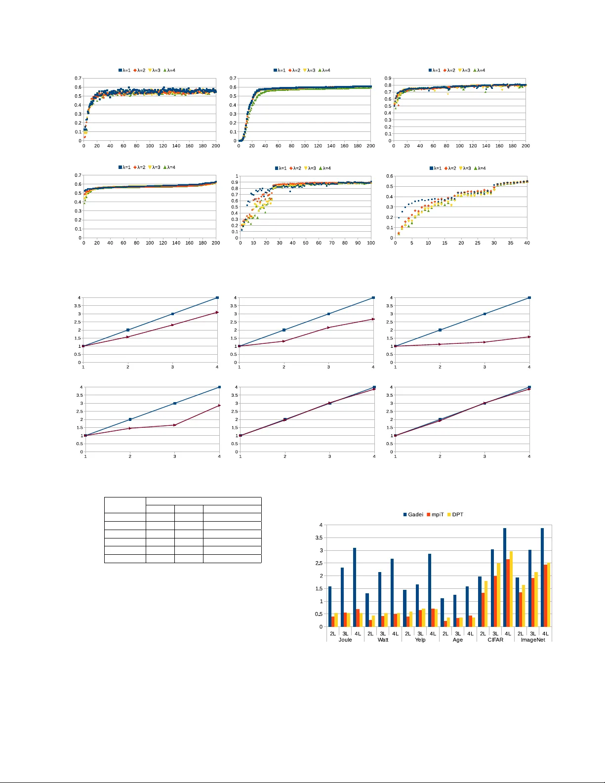
Comments & Academic Discussion
Loading comments...
Leave a Comment