Convolutional RNN: an Enhanced Model for Extracting Features from Sequential Data

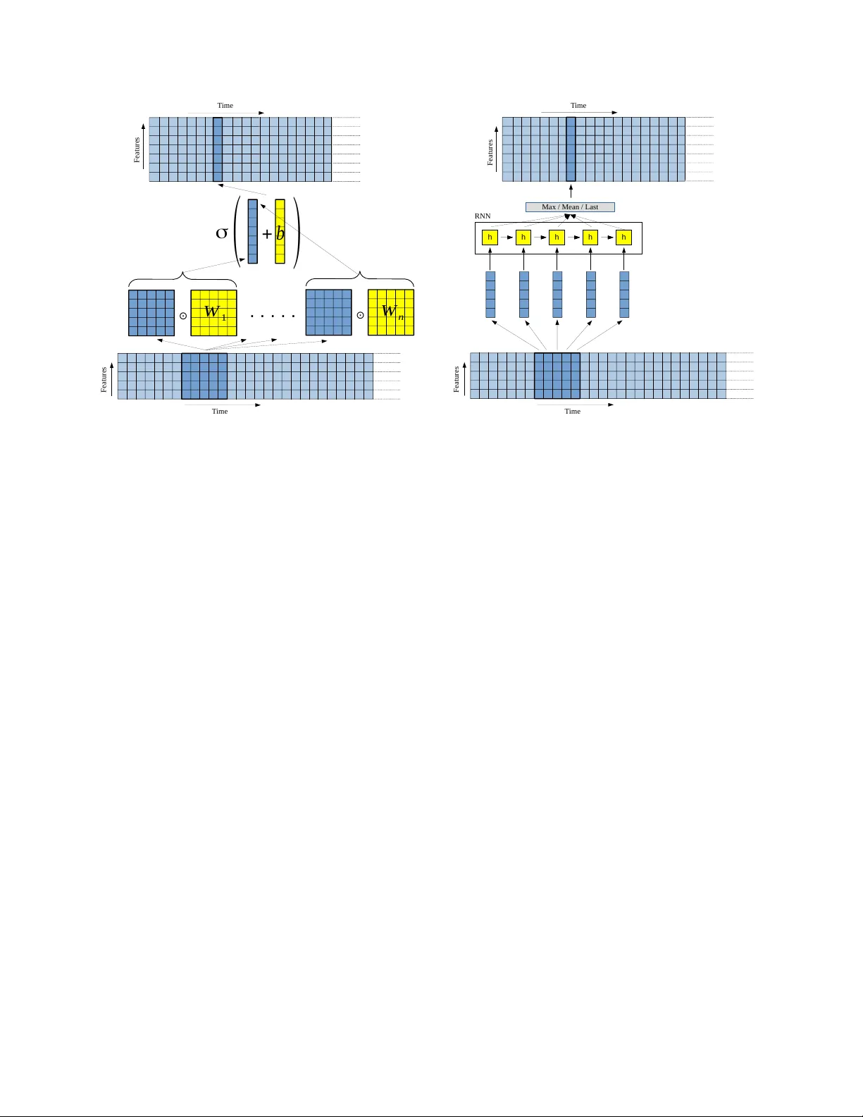
Con v olutional RNN: an Enhanced Model for Extracting Features from Sequential Data Gil K eren Chair of Complex and Intelligent systems Univ ersity of Passau Passau, German y cruvadom@gmail.com Bj ¨ orn Schuller Chair of Complex and Intelligent systems Univ ersity of Passau Passau, German y , Machine Learning Group Imperial College London, U.K. schuller@ieee.org Abstract —T raditional con volutional layers extract features from patches of data by applying a non-linearity on an affine function of the input. W e propose a model that enhances this fea- ture extraction process for the case of sequential data, by feeding patches of the data into a recurr ent neural network and using the outputs or hidden states of the recurrent units to compute the extracted features. By doing so, we exploit the fact that a window containing a few frames of the sequential data is a sequence itself and this additional structure might encapsulate valuable information. In addition, we allow for more steps of computation in the feature extraction process, which is potentially beneficial as an affine function follo wed by a non-linearity can result in too simple features. Using our con volutional recurr ent layers, we obtain an improv ement in performance in two audio classification tasks, compar ed to traditional con volutional layers. Tensorflow code for the conv olutional r ecurrent layers is publicly available in https://github .com/cruvadom/Con volutional- RNN. I . I N T R O D U C T I O N Over the last years, Con v olutional Neural Networks (CNN) [1] ha ve yielded state-of-the-art results for a wide variety of tasks in the field of computer vision, such as object classification [2], traf fic sign recognition [3] and image caption generation [4]. The use of CNN was not limited to the field of computer vision, and these models were adapted successfully to a v ariety of audio processing and natural language pro- cessing tasks such as speech recognition [5], [6] and sentence classification [7]. When applying a con volutional layer on some data, this layer is extracting features from local patches of the data and often is followed by a pooling mechanism to pool v alues of features o ver neighboring patches. The e xtracted features can be the input of the next layer in a neural network, possibly another con volutional layer or a classifier . Models using con volutional layers for extracting features from raw data can outperform models using hand-crafted features and achiev e state-of-the-art-results, such as in [2], [6]. Recurrent Neural networks (RNN), are models for process- ing sequential data which is often of a varied length such as text or sound. Long-Short T erm Memory networks (LSTM) [8] are a special kind of recurrent neural networks that use a gating mechanism for better modeling of long-term dependencies in the data. These models hav e been used successfully for speech recognition [9] and machine translation [10] [11]. When the data is a sequence of frames and of a varied length, a model combining both, conv olutional layers and recurrent layers, can be constructed in the follo wing way: the con volutional layers are used to extract features from data patches that in this case are windo ws comprised of a few consecutiv e frames in the sequence. These features extracted from windo ws are another time sequence, which can be the input of another con volutional layer , or finally the input of a recurrent layer that models the temporal relations in the data. One additional benefit of this method is that using a pooling mechanism after the conv olutional layer can shorten the input sequence to the recurrent layer, so that the recurrent layers will need to model temporal dependencies ov er a smaller number of frames. A possible limitation of traditional con volutional layers is that they use a non-linearity applied on affine functions to extract features from the data. Specifically , an extracted feature is calculated by element-wise multiplication of a data patch by a weight matrix, summing the product ov er all elements of the matrix, adding a bias scalar, and applying a non-linear function. Theoretically , the function that maps a data patch to a scalar feature v alue can be of arbitrary complexity and it is plausible that in order to achiev e a better representation of the input data, a more complicated non-linear functions can be used (i.e., with more layers of computation). Note that simply stacking more conv olutional layers with kernel sizes bigger than 1 × 1 does not solve this issue, because a consequent layer will mix the outputs of the previous layer for different locations and will not exhibit the potentially wanted behavior of extracting more complicated features from a data patch using only this data patch itself. In the case of sequential data, windows of a few consecutiv e data frames have an additional property: ev ery window is itself a small sequence comprised of a few frames. This additional property can be potentially exploited in order to e xtract better features from the windows. In this work, we introduce the CRNN (Con volutional Recurrent Neural Network) model that feeds ev ery window frame by frame into a recurrent layer and use the outputs and hidden states of the recurrent units in each frame for extracting features from the sequential windows. By doing so, our main contribution is that we can potentially get better features in comparison to the standard con volutional layers, as we use additional information about each windo w (the temporal information) and as the features are created from the dif ferent windo ws using a more complicated function in comparison to the traditional conv olutional layers (more steps of computation). W e perform experiments on different audio classification tasks to compare a few v ariants of our proposed model to gain improv ement in classification rates ov er models using traditional conv olutional layers. The rest of the paper is organized as follows. In Section II we briefly discuss related work. In Section III we describe how we extract features using recurrent layers and in Section IV we conduct experiments on audio data classification using our proposed models. In section V we discuss possible explanations for the observed results and conclude the work in Section VI. I I . R E L A T E D W O R K As described above, the feature extraction process of a standard con volutional layer can potentially be too simple, as it is simply the application of a non-linearity on an affine function of the data patch. In [12], the authors address this issue by replacing the affine function for e xtracting features by a multilayer feedforward neural network to get state-of-the- art results on a few object classification datasets, but they only allow for a feedforward feature extraction process and not a recurrent one. Few other works attempt to extract features from patches of data by using the hidden states of the recurrent layer . In [13] the authors extract features from an image path by using a recurrent layer that takes at every time step as input this image path and the output of the last time step. This approach can result in better features as creating them using a recurrent network is a more complicated process (i.e., with more steps of computation), but still, there is no use of a sequential nature of the data patches themselv es, and the process can be very computationally e xpensive as the same path is fed ov er and ov er to the recurrent net. In a recent work [14], the authors split an image into a grid of patches, and scan ev ery column in both directions with two recurrent networks, feeding into each recurrent network one image patch at a time. The acti vations of the recurrent units in both recurrent networks after processing a specific patch are concatenated and used as inputs for another two recurrent networks that now scan each row of patches in both directions. The activ ations of the recurrent units after processing a specific patch in the last two recurrent networks are concatenated and used as the input for the next layer or a classifier . This approach indeed uses hidden states of a recurrent network as extracted features, but there are a few major differences between this approach and our proposed approach. First, it is important to note that the usage of recurrent networks for sequential data is natural while using recurrent networks for images can be problematic because of the lack of natural sequences in the data. Another major difference is that in [14] each data path is fed in one piece to the recurrent layer and there is no usage of a sequential nature of the patches themselves. In addition, in [14] there is no option for o verlapping patches to account for small translations in the data. I I I . C O N V O L U T I O N A L L O N G S H O RT T E R M M E M O RY A. Extracting local featur es W e describe a general structure for a layer extracting (pooled) temporally local features from a data set of se- quences. Using this terminology , both, traditional conv olu- tional layers [1] and our method of Con volutional Recurrent Neural Network, (CRNN) can be described. Assume a labeled dataset where each example in the dataset is a sequence of a varied number of frames and all frames hav e the same fixed number of features. Denote x an example from the dataset, l the number of frames in the sequence x and k the number of features in each frame in each example in the dataset, so x is of size k × l . Note that for simplicity we assume each frame contains a one-dimensional feature vector of length k , but this can be easily generalized to the case of multidimensional data in each frame (such as video data) by flattening this data into one dimension. From the sequence x we create a sequence of windows, each windo w comprised of r 1 consecutiv e frames. Then, each window is of size k × r 1 , and we take a shift of r 2 frames between the starting point of two consecutiv e windows. Ne xt, we apply a features extraction function f on each windo w to get a set of n features describing each windo w , meaning that the feature vector of size n describing a window w is f ( w ) . Applying f on each windo w results in another sequence x 0 in which ev ery frame is represented with n features. Finally , for pooling, we create windo ws of size n × p 1 from the sequence x 0 in the same way we created windo ws from the sequence x , with a shift of p 2 frames between the starting points of two consecuti ve windows, and we perform max-pooling across frames (for each feature separately) in each window to transform windo ws of size n × p 1 to a vector of size n × 1 . After applying max-pooling to each window the resulting sequence contains (pooled) temporally local features of the sequence x extracted by the function f and can be fed into the next layer in the network or a classifier . B. Long Short T erm Memory networks and Bidir ectional Long Short T erm Memory networks A simple recurrent neural network takes a sequence ( x 1 , . . . , x t ) and produces a sequence ( h 1 , . . . , h t ) of hidden states and a sequence ( y 1 , . . . , y t ) of outputs in the follo wing way: h t = σ ( W xh x t + W hh h t − 1 + b h ) (1) y t = W hy h t + b y , (2) where σ is the logistic sigmoid function, W xh , W hh , W hy are weight matrices and b h , b y are biases. Long Short T erm Memory netw orks [8] are a special kind of recurrent neural networks (RNN) that use a gating mechanism to allo w better modeling of long-term dependencies in the data. T i me F e a t u r e s F e a t u r e s T im e ⊙ W 1 + . . . . . ⊙ W n b ( ) σ (a) Extraction of features from a time window using a standard conv o- lutional layer . For each feature the time window is multiplied element- wise by a different matrix. This product is summed and added to a bias term and then a non-linearity is applied. Here  denotes an element-wise multiplication follo wed by summation. T ime F e a t u r e s h h h h h h h h h h h h h h h F e a t u r e s T im e RN N Max / M e an / La s t (b) Extraction of features from a time window using a CRNN layer . First, the time window is fed frame by frame into a recurrent layer. Then, the hidden states of the recurrent layer along the dif ferent frames of the window are used to compute the extracted features, by applying a max/mean operator or simply by taking the vector of hidden states of the last time frame in the window . Note that it is possible to extract features from the window using the outputs of the recurrent layer in each time step instead of the hidden states. Fig. 1. Extraction of features from a time window by a traditional conv olutional layer (a) and a CRNN layer (b). The v ersion of LSTM used in this paper [15] is implemented by replacing Equation 1 with the following steps: i t = σ ( W xi x t + W hi h t − 1 + W ci c t − 1 + b i ) (3) f t = σ ( W xf x t + W hf h t − 1 + W cf c t − 1 + b f ) (4) c t = f t c t − 1 + i t tanh ( W xc x t + W hc h t − 1 + b c ) (5) o t = σ ( W xo x t + W ho h t − 1 + W co c t + b o ) (6) h t = o t tanh ( c t ) , (7) where σ is the logistic sigmoid function, i, f , o are the input, forget and output gates’ acti v ation vectors, and c, h are cell and hidden states vectors. Since the standard LSTM processes the input only in one direction, an enhancement of this model was proposed [16], namely Bidirectional LSTM (BLSTM), in which the input is processed both in the standard order and rev ersed order, allowing to combine future and past information in ev ery time step. A BLSTM layer comprises of two LSTM layers processing the input separately to produce − → h , − → c , the hidden and cell states of an LSTM processing the input in the standard order , and ← − h , ← − c , the hidden and cell states of an LSTM processing the input in rev ersed order . Both, − → h and ← − h , are then combined: y t = W − → h y − → h t + W ← − h y ← − h t + b y , (8) to produce the output sequence of the BLSTM layer . Note that it is possible to use the cell states instead of the hidden states of the two LSTM layers in an BLSTM layer , in the following way: y t = W − → c y − → c t + W ← − c y ← − c t + b y , (9) to produce the the output sequence of the BLSTM layer . C. Con volutional layers and Con volutional Recurrent layers T raditional con volutional layers (with max-pooling) can be described using the terms from Section III-A by setting the function f extracting n features from a data patch w : f ( w ) = ( σ ( sum ( W 1  w ) + b 1 ) , . . . , σ ( sum ( W n  w ) + b n )) , where W 1 , . . . , W n are weight matrices, b 1 , . . . , b n are biases,  is an element-wise multiplication, and sum is an operator that sums all elements of a matrix. This giv es rise to n different features computed for each window using the n weight matrices and biases. The values of a specific feature across windo ws is traditionally called a feature map. Figure 1a depicts the feature extraction procedure in a standard con volutional layer . Next, we describe our proposed model, Con volutional Re- current Neural Network (CRNN), and as special cases Con- volutional Long Short T erm Memory (CLSTM) and Con vo- lutional Bidirectional Long Short T erm Memory (CBLSTM), by describing the feature extraction function f ( w ) that corre- sponds to these layers. A CRNN layer takes advantage of the fact that ev ery window w of size k × r 1 can also be interpreted as a short time sequence of r 1 frames, each of size k × 1 . Using this fact, we can feed a window w as a sequence of r 1 frames into an RNN. The RNN then produces a sequence of hidden states ( h 1 , . . . , h r 1 ) in which each element is of size n × 1 , where n is the number of units in the RNN layer . Finally , in order to create the feature vector of length n that represents a window w , we can either set f ( w ) to be the mean or max ov er vectors of the sequence ( h 1 , . . . , h r 1 ) (computing mean or max for each feature separately), or simply set f ( w ) to be the last element of the sequence. Figure 1b depicts the feature creation process in a CRNN layer . As special case of CRNN we ha ve the CLSTM and CBLSTM, in which the RNN layer is an LSTM or BLSTM, respectiv ely . Note that we use the same RNN layer to compute f ( w ) for all windo ws w , meaning that as in a con volutional layer, we use the same v alues of parameters of the model to extract local features for all windows. In addition, note that the RNN may produce two additional sequences, a sequence of outputs ( y 1 , . . . , y r 1 ) and a sequence of cell states ( c 1 , . . . c r 1 ) (in the case of CLSTM or BLSTM) that can be used instead of the hidden states sequence to compute the features representing a window . In case we use the sequence of outputs, the hidden dimension of the recurrent layer is free of constraints. W e propose another extension for the CL TSM layer , namely the Extended CLSTM layer . In Extended CLSTM, we want to allow an LSTM layer to use the additional information about the position of each frame inside the time window . In a standard LSTM this is not possible, since all frames being fed into the LSTM are using the same weight matrices W xi , W xf , W xc , W xo from equations 3, 4, 5 and 6. Therefore, in an Extended CLSTM layer we use a different copy of each of the abov e four matrices for each frame in the window . I V . E X P E R I M E N T S A. Experiments on emotion classification: F A U-Aibo corpus The F A U Aibo Emotion Corpus [17] contains audio record- ings of children interacting with Son y’ s pet robot Aibo. The corpus consists of spontaneous German speech where emo- tions are expressed. W e use the same train and test subsets and labels as were used in the Interspeech 2009 Emotion Challenge [18]. The corpus contains about 9.2 hours of speech, where the train set comprises of 9,959 examples from 26 children (13 male, 13 female) and the test set comprises of 8,257 examples from 25 children (8 male, 17 female). The train and test subsets are speaker-independent. A subset of the training set containing utterances from the first fiv e speakers (according to the dataset’ s speaker IDs) was used as a validation set and utterances from these fi ve speakers were not used for training the model. The dataset is labeled according to the emotion demonstrated in each utterance, and there exist two versions for labels of this dataset. In the fiv e labels version, each utterance in the corpus is labeled with one of: A N G E R , E M P H A T I C , N E U T R A L , P O S I T I V E , R E S T . In the two labels version, each utterance in the corpus is labeled either as N E G AT I V E or I D L E . Since each class has a different number of instances, we add to the training set random examples from the smaller classes until the size of all classes is equal, in a way such that no example was duplicated twice before all examples from the same class were duplicated once. W e trained the models to classify the correct emotion exhibited in each utterance. The input features used for the experiments is 26-dimensional log mel filter -banks, computed with windows of 25 ms with a 10 ms shift. W e distinguish the term input features , which is used to denote the input data representation (here, log mel filter-banks), from the term featur es or e xtracted featur es , which we use to describe the output of the various con volutional layers. W e applied a mean and standard de viation normalization for each combination of speaker and feature independently . The baseline model we used contains one LSTM layer of dimension 256. F or e very utterance, the hidden states of the LSTM layer in each time frame were fed into a dense layer with 400 Rectified Linear Units [19] and the outputs of the latter were fed to a softmax layer [20]. The outputs of the softmax layer in the last four time steps of each utterance were av eraged, and the class with the highest av eraged probability was selected as the prediction of the model. In addition, we ev aluated models containing con v olutional layers preceding the above described model, of three types: standard conv olutional layers, CLSTM and Extended CLSTM. In these models, the features were first fed into two con- secutiv e con volutional layers, each with a windo w size of 5 time frames, with a shift of 2 time frames between the starting points of consecutive windows. For the CLSTM and the Extended CLSTM layers, the output of the layers for each window was c 5 , the cell states vector of the last time frame in each window . For each windo w , each layer extracts 100 features (therefore the dimension of the CLSTM and Extended CLSTM layers was 100). Each con volutional layer also included max-pooling over the features extracted from groups of two windows, with a shift of two windows between consecutiv e pooling groups (the max-pooling operator was computed for each feature separately). The parameters were learned in an end-to-end manner , meaning that all parameters of the model were optimized simultaneously , using the Adam optimization method [21] with learning rate of 0 . 002 , β 1 = 0 . 1 and β 2 = 0 . 001 (hyper- parameters of the Adam optimization method) to minimize a cross-entropy objective. Note that we did not use Back Propagation Thorough Time (BPTT) [22] and we used only the outputs of the last four time steps to compute the model predictions. This approach can potentially result in a difficulty in optimizing, as we back propagate through a very deep network. This potential problem is alleviated by the fact that using two con volutional layers makes the output sequence shorter and therefore helps ov ercoming this obstacle, and we did not observe any exceptional difficulties in learning the model in an end-to-end manner . The selected model used on the test set is the one with best T ABLE I R E S U L T S O N E M OT I O N C L AS S I FI C ATI O N T A S K ( B E S T R E S U L T S I N B O L D ) T est set UA Recall [%] 2 labels 5 labels baseline 69 . 01 ± 0 . 93 36 . 89 ± 1 . 8 standard con volutional layer 69 . 13 ± 0 . 87 38 . 22 ± 1 . 19 CLSTM 70.59 ± 0.58 39 . 41 ± 0 . 57 Extended CLSTM 69 . 85 ± 0 . 38 39.72 ± 0.2 misclassification rate on the validation set, and training was stopped after 12 epochs of training without improv ement of the misclassification rate of the v alidation set. The experiments were performed using the deep learning framework Blocks [23] based on Theano [24], [25]. Results on the test set using the baseline model and using the different types of conv o- lutional layers are reported in T able I. Since the number of utterances from each class may vary , we report the Unweighted A verage (UA) Recall, which is the official benchmark measure on this task. The U A Recall is defined to be 1 n n X i =1 r i , where n is the number of classes, and the recall r i is the number of correctly classified examples from class i (true positiv es) divided by the total number of examples from class i . As seen in the results, our models outperform both the baseline and traditional con volutional layers for this task, as well as the challenge’ s baseline [18]. B. Experiments on age and gender classification: aGender corpus The aGender corpus [26] contains audio recordings of predefined utterances and free speech produced by humans of different age and gender . Each utterance is labeled as one of four age groups: C H I L D , Y O U T H , A D U LT , S E N I O R , and as one of three gender classes: F E M A L E , M A L E and C H I L D . For the train and validation sets, we split the train set from the Interspeech 2010 Paralinguistic Challenge [27] which contains 32,527 utterances in 23.43 hours of speech by 471 speakers. W e split this set by selecting random 20 speakers (speaker IDs can be obtained from www .openaudio.eu) from each one of the sev en groups (child, youth male, youth female, adult male, adult female, senior male, senior female) and using all utterances from these 140 speakers as a validation set. Utterances from the rest of the speakers were used as the train set. The test set we used is the set used as the development set in the Interspeech 2010 Paralinguistic Challenge and contains 20,549 utterances in 14.73 hours of speech by 299 speakers. The train, validation and test sets are speaker independent (i.e., each speaker appears in exactly one of the sets). W e use this data for two tasks: age classification and gender classification. For each task, we balance the number of instances between the different classes in the same way we did with the F A U-Aibo dataset. In these experiments with age and and gender classifica- tion, we ev aluated our models using two different sets of input features. The first set of input features used is 26- dimensional log mel filter-banks, computed with windows of 25 ms with a 10 ms shift. The second set of input features is the extended Gene va Minimalistic Acoustic Parameter Set (eGeMAPS) [28], a input features set suited for voice research and specifically paralinguistic research, containing 25 LLDs such as pitch, jitter , center frequenc y of formants, shimmer , loudness, alpha ratio, spectral slope and more. The eGeMAPS input features were extracted using the openSMILE toolkit [29], again with 25 ms windows with a 10 ms shift. For each feature set we applied mean and standard deviation normalization for each combination of speaker and feature independently . The models we ev aluated contain a few dif ferences com- pared to the models used for emotion recognition. Our baseline model contains one BLSTM layer that allows to use past and future information in each time step. Inside the BLSTM layer , there are two LSTM layers (forward and backward) of dimension 256 each. As in Equation 8, in every time step the hidden states of the two LSTM layers were fed into a dense layer of dimension 400, followed by the Rectified Linear non-linearity , that in turn was fed into a softmax layer . The outputs of the softmax layer were av eraged across all time steps, and the class with the highest probability was selected as the prediction of the model. W e also ev aluated models with one con volutional layer preceding the above described model, of three types: standard con volutional layer, CLSTM and CBLSTM, with window sizes, pooling sizes, shifts and number of extracted features identical to the layers in the emotion recognition experiments in Section IV -A. The output of the CLSTM layer for each window was max ( c 1 , . . . , c 5 ) where the max operator is computed for each feature separately . Inside the CBLSTM layer , each LSTM layer was of dimension 100 and the cell states of the two LSTM layers were combined to produce an output y t of size 100 in each time step t as in Equation 9. The output of the CBLSTM layer for each window was then max ( y 1 , . . . , y 5 ) where the max operator is computed for each feature separately . The rest of the training setting is identical to the emotion recognition experiments. Again, we did not use BPTT [22]. The fact that in these experiments we used all time steps to compute the prediction of the model makes it easier to learn the model in an end-to-end manner , as it creates a shorter path between the input and the output of the model. Unweighted A verage (U A) Recall on our test set is reported in tables II and III, which is the official benchmark measure on this task. As seen in the results, the model with the CBLSTM layer yields an improvement ov er the baseline, traditional con volutional and CLSTM layers for this task, using both sets of input features. In addition, in most cases the model with the CLSTM layer outperforms our baseline and the standard con volutional layer , as well as the challenge’ s baseline [27] (for the the challenge’ s baseline, using the eGeMAPS input T ABLE II R E S U L T S O N G E N D E R C L A S S I FI C A T I O N ( B E S T R E S U LTS I N B O L D ) T est set UA Recall [%] log mel filter-banks eGeMAPS baseline 70 . 94 ± 1 . 0 76 . 96 ± 0 . 4 standard con volutional layer 74 . 49 ± 0 . 21 77 . 54 ± 0 . 3 CLSTM 75 . 68 ± 0 . 7 78 . 17 ± 0 . 33 CBLSTM 76.03 ± 1.28 78.23 ± 0.49 T ABLE III R E S U L T S O N AG E C L A S S I FIC AT IO N ( B E S T R E S U LTS I N B O L D ) T est set UA Recall [%] log mel filter-banks eGeMAPS baseline 43 . 14 ± 0 . 94 46 . 51 ± 0 . 62 standard con volutional layer 45 . 93 ± 0 . 52 47 . 09 ± 0 . 76 CLSTM 45 . 51 ± 0 . 27 47 . 15 ± 0 . 57 CBLSTM 46.39 ± 0.14 47.29 ± 0.58 features). C. Comparing Differ ent CLSTM ar chitectur es When implementing a CLSTM model, one has two choices to make regarding the specific architecture. First, for feature extraction, one can use the sequence ( h 1 , . . . , h n ) of hidden states, the sequence ( c 1 , . . . , c n ) of cell states or the sequence ( y 1 , . . . , y n ) of outputs. The second choice to be made is whether to apply the max or mean operators on the selected sequence (applied to each feature independently) or simply to use the last element of the selected sequence as the extracted features. Using the max operator ov er a group of objects as the output of a layer seems to yield good results in Deep Learning in different situations such as con volutional layers with max- pooling [30] [31] or Maxout Netw orks [32]. The max operator has some desired theoretical properties as well. For example, in [32] the authors show that applying the max operator over a sufficiently high number of linear functions can approximate an arbitrary con vex function. Usage of the mean operator has been made in Deep Learning as well, when applying mean pooling with con volutional layers [33]. W e empirically ev aluated six dif ferent implementations of the CLSTM model, by using the two sequences ( h 1 , . . . , h n ) and ( c 1 , . . . , c n ) of hidden and cell states, each with the three operations: max , mean and using the last. W e compared the different implementations of the CLSTM model both on the emotion classification task and the age and gender classification task. For both tasks, as introduced in Section IV -A and Section IV -B, we used the 26-dimensional log mel filter-banks as the input features. For each task we used the same network architecture and training procedure as was used in the abov e experiments, with the only difference being the implementation of the CLSTM layers (as in the e xperiments abov e, the emotion classification model contains two CLSTM layers, and the age and gender classification model contains one CLSTM layer). T able IV contains the result for these experiments. W e observed that in all four tasks, the average results of implementations using the cell states is better than the average results of implementations using the hidden states, but still in one task of the four the implementation yielding the best result used the hidden states. The results regarding which one of the six dif ferent implementations is preferable are ambiguous, and we cannot point out one implementation which is better than the others. In addition, comparing the usage of max , mean and the last v ector of a sequence also gav e ambiguous results, with a slight preference towards using the max operator . V . D I S C U S S I O N W e observed that the CBLSTM outperformed the CLSTM layer in classifying age and gender of speakers. This result can have sev eral explanations. First, when feeding a window to a CBLSTM layer , both past and future information can be used in each time step, a property that does not exist in the CLSTM layer , which processes the window in one direction only . The future information might be valuable when analyzing audio data and in particular when classifying the age and gender of a speaker , and this might explain why the CBLSTM layers performed better compared to the CLSTM layers. Another phenomenon that might help explaining the difference between CBLSTM and CLSTM is the follo wing: when we used a CLSTM layer, we computed features for a window by applying a max operator on the sequence of cell states. The cell states then hav e to play a double role: on the one hand, they ha ve to contain valuable data to feed to the next time step and on the other hand, they hav e to contain valuable data to feed the next layer or the classifier . These two requirements can potentially contradict each other and this may hamper the performance of a CLSTM model. When we used the CBLSTM layers, we combined the cell activ ations of the forward and backward LSTM layers using weight matrices to compute the output y t in each time step as in Equation 9, and we used y t to compute the e xtracted features for the window . By doing that, we achiev e two things: we allow for an additional transformation on the cell states before using them for computing the extracted features, and we get a separation of the two potentially contradicting roles of the cell states described abov e. In recent years, some works perform audio related tasks such as speech recognition using the raw wav eform [5], [34], [35]. For these models, the sequences can be relativ ely long and conv olutional layers might be applied on windows containing many time steps. In that case, the CRNN model can be especially useful, because of two reasons: first, longer windows encapsulate more temporal structure that might con- tain valuable information. Second, while in traditional conv o- lutional layers the number of parameters grows with the size of window , in the CRNN model the number of parameters does not depend on the length of the window (except in the extended CLSTM model) but only on the number of features per time step and the inner dimension of the CRNN layer . T ABLE IV D I FF E R EN T I M P L E M EN TA T I O N S O F C L S T M ( B E S T R E S U LTS I N B O L D ) . D E TA I L S I N T H E T E X T . T est set UA Recall [%] Emotion 2 classes Emotion 5 classes Age Gender A verage hidden states, mean 70 . 04 ± 0 . 37 39 . 47 ± 0 . 74 45 . 62 ± 1 . 08 74 . 54 ± 0 . 55 57 . 42 hidden states, max 70 . 2 ± 0 . 46 39 . 46 ± 1 . 06 45 . 89 ± 1 . 13 75 . 02 ± 1 . 23 57 . 64 hidden states, last 70 . 06 ± 0 . 3 40.47 ± 1.02 45 . 53 ± 0 . 53 74 . 73 ± 1 . 55 57 . 7 cell states, mean 70 . 15 ± 0 . 43 40 . 27 ± 1 . 29 46.2 ± 0.33 75 . 26 ± 0 . 14 57.97 cell states, max 70 . 51 ± 0 . 18 39 . 99 ± 0 . 76 45 . 51 ± 0 . 27 75.68 ± 0.7 57 . 92 cell states, last 70.59 ± 0.58 39 . 41 ± 0 . 57 45 . 67 ± 0 . 72 74 . 79 ± 1 . 11 57 . 62 mean 70 . 10 39 . 87 45.91 74 . 90 57 . 70 max 70.35 39 . 73 45 . 70 75.35 57.78 last 70 . 33 39.94 45 . 61 74 . 76 57 . 66 hidden states 70 . 10 39 . 80 45 . 69 74 . 76 57 . 59 cell states 70.42 39.89 45.79 75.24 57.84 Another observation from the results is that the hand-crafted input features set eGeMAPS performed better than the low complexity log mel filter-banks. This is in contrary to results from the field of computer vision and speech recognition, where in the recent years features extracted from raw data by conv olutional layers outperform hand-crafted input features and achiev e state-of-the-art results in various tasks. W e con- jecture that with bigger datasets and further dev elopment of models, simpler input features will outperform hand-crafted input features for the tasks we experimented with. V I . C O N C L U S I O N W e have proposed the CRNN model, to improv e the process of feature extraction from windo ws of sequential data that is being performed by traditional con volutional networks, by exploiting the additional temporal structure that each window of data encapsulates. The CRNN model extracts the features by feeding a window frame-by-frame to a recurrent layer , and the hidden states or outputs (or cell states in case of an LSTM) of the recurrent layer are then used to compute the extracted features for the window . By doing so, we also allow for more layers of computation in the feature generation process, which is potentially beneficial. W e experimented with three types of the CRNN model, namely CLSTM, Extended CLSTM and CBLSTM. W e found that these models yield improvements in classification results compared to the traditional con volutional layers for the same number of extracted features. The improv ements in classification results were observed when the input data comprised of log mel filter-banks, which are features of low comple xity , and e ven when the input data comprised of higher level properties of the audio signal (the eGeMAPS features), the model could still extract v aluable information from the data and an improv ement in classification result was obtained. In future work, futures extracted by the CRNN model can be further ev aluated and compared to features extracted by standard conv olutional layers. In addition, the CRNN model can be used in larger models and for v arious applications, such as speech recognition and video classification. A C K N O W L E D G M E N T This work has been supported by the European Com- munity’ s Sev enth Framework Programme through the ERC Starting Grant No. 338164 (iHEARu). W e further thank the NVIDIA Corporation for their support of this research by T esla K40-type GPU donation. R E F E R E N C E S [1] Y . LeCun, B. Boser, J. S. Denker, D. Henderson, R. E. Howard, W . Hubbard, and L. D. Jackel, “Backpropagation applied to handwritten zip code recognition, ” Neural computation , vol. 1, no. 4, pp. 541–551, 1989. [2] A. Krizhevsk y , I. Sutskever , and G. E. Hinton, “Imagenet classification with deep con volutional neural networks, ” in Pr oc. of Advances in neural information pr ocessing systems (NIPS) , Lake T ahoe, NV , 2012, pp. 1097–1105. [3] D. Ciresan, U. Meier, and J. Schmidhuber, “Multi-column deep neural networks for image classification, ” in Pr oc. of the IEEE Confer ence on Computer V ision and P attern Recognition (CVPR) , Providence, RI, 2012, pp. 3642–3649. [4] O. V inyals, A. T oshev , S. Bengio, and D. Erhan, “Show and tell: A neural image caption generator, ” in Pr oc. of the IEEE Confer ence on Computer V ision and P attern Recognition (CVPR) , Boston, MA, 2015, pp. 3156–3164. [5] T . N. Sainath, R. J. W eiss, A. Senior , K. W . W ilson, and O. V inyals, “Learning the speech front-end with raw wav eform CLDNNs, ” in Pr oc. of INTERSPEECH 2015, 16th Annual Confer ence of the International Speech Communication Association , Dresden, Germany , 2015, pp. 1–5. [6] D. Amodei, R. Anubhai, E. Battenberg, C. Case, J. Casper , B. C. Catanzaro, J. Chen, M. Chrzanowski, A. Coates, G. Diamos, E. Elsen, J. Engel, L. Fan, C. Fougner , T . Han, A. Y . Hannun, B. Jun, P . LeGresley , L. Lin, S. Narang, A. Y . Ng, S. Ozair , R. Prenger , J. Raiman, S. Satheesh, D. Seetapun, S. Sengupta, Y . W ang, Z. W ang, C. W ang, B. Xiao, D. Y ogatama, J. Zhan, and Z. Zhu, “Deep speech 2: End-to-end speech recognition in English and Mandarin, ” arXiv preprint , 2015. [7] Y . Kim, “Conv olutional neural networks for sentence classification, ” in Pr oc. of the 2014 Conference on Empirical Methods in Natur al Language Pr ocessing (EMNLP) , Doha, Qatar , 2014, pp. 1746–1751. [8] S. Hochreiter and J. Schmidhuber, “Long short-term memory , ” Neural computation , vol. 9, no. 8, pp. 1735–1780, 1997. [9] A. Graves, A. Mohamed, and G. E. Hinton, “Speech recognition with deep recurrent neural networks, ” in Pr oc of. the IEEE International Confer ence on Acoustics, Speech and Signal Pr ocessing, (ICASSP) , V ancouver , Canada, 2013, pp. 6645–6649. [10] K. Cho, B. V an Merri ¨ enboer , C ¸ . G ¨ ulc ¸ ehre, D. Bahdanau, F . Bougares, H. Schwenk, and Y . Bengio, “Learning phrase representations using RNN encoder–decoder for statistical machine translation, ” in Pr oc. of the 2014 Confer ence on Empirical Methods in Natur al Language Pr ocessing (EMNLP) , Doha, Qatar, Oct. 2014, pp. 1724–1734. [11] I. Sutskever , O. V inyals, and Q. V . Le, “Sequence to sequence learning with neural networks, ” in Pr oc. of Advances in neural information pr ocessing systems (NIPS) , Montreal, Canada, 2014, pp. 3104–3112. [12] M. Lin, Q. Chen, and S. Y an, “Network in network, ” arXiv preprint arXiv:1312.4400 , 2013. [13] M. Liang and X. Hu, “Recurrent conv olutional neural network for object recognition, ” in Proc. of the IEEE Conference on Computer V ision and P attern Recognition (CVPR) , Boston, MA, 2015, pp. 3367–3375. [14] F . V isin, K. Kastner, K. Cho, M. Matteucci, A. Courville, and Y . Bengio, “Renet: A recurrent neural network based alternativ e to con volutional networks, ” arXiv pr eprint arXiv:1505.00393 , 2015. [15] F . A. Gers, N. N. Schraudolph, and J. Schmidhuber, “Learning precise timing with LSTM recurrent networks, ” The J ournal of Machine Learn- ing Resear ch (JMLR) , vol. 3, pp. 115–143, 2003. [16] M. Schuster and K. K. Paliwal, “Bidirectional recurrent neural net- works, ” Signal Pr ocessing, IEEE T ransactions on , vol. 45, no. 11, pp. 2673–2681, 1997. [17] S. Steidl, “ Automatic classification of emotion related user states in spontaneous children’ s speech, ” Ph.D. dissertation, University of Erlangen-Nuremberg, 2009. [18] B. Schuller , S. Steidl, and A. Batliner, “The INTERSPEECH 2009 emotion challenge, ” in Pr oc. of INTERSPEECH 2009, 10th Annual Confer ence of the International Speech Communication Association , Brighton, UK, 2009, pp. 312–315. [19] V . Nair and G. E. Hinton, “Rectified linear units impro ve restricted boltzmann machines, ” in Pr oc. of the 27th International Confer ence on Machine Learning (ICML) , Haifa, Israel, 2010, pp. 807–814. [20] J. S. Bridle, “Probabilistic interpretation of feedforward classification network outputs, with relationships to statistical pattern recognition, ” in Neur ocomputing . Springer , 1990, pp. 227–236. [21] D. Kingma and J. Ba, “ Adam: A method for stochastic optimization, ” in Pr oc. of International Confer ence on Learning Repr esentations (ICLR) , San Diego, CA, 2015. [22] P . J. W erbos, “Backpropagation through time: what it does and how to do it, ” Pr oceedings of the IEEE , vol. 78, no. 10, pp. 1550–1560, 1990. [23] B. van Merri ¨ enboer , D. Bahdanau, V . Dumoulin, D. Serdyuk, D. W arde- Farley , J. Chorowski, and Y . Bengio, “Blocks and Fuel: Frameworks for deep learning, ” arXiv preprint , 2015. [24] F . Bastien, P . Lamblin, R. Pascanu, J. Bergstra, I. J. Goodfellow , A. Bergeron, N. Bouchard, and Y . Bengio, “Theano: new features and speed impro vements, ” Deep Learning and Unsupervised Feature Learning W orkshop, Advances in neural information processing systems (NIPS), 2012. [25] J. Bergstra, O. Breuleux, F . Bastien, P . Lamblin, R. Pascanu, G. Des- jardins, J. Turian, D. W arde-Farley , and Y . Bengio, “Theano: a CPU and GPU math expression compiler , ” in Pr oc. of the Python for Scientific Computing Confer ence (SciPy) , vol. 4, 2010, p. 3. [26] F . Burkhardt, M. Eckert, W . Johannsen, and J. Stegmann, “ A database of age and gender annotated telephone speech, ” in Pr oc. of the International Confer ence on Language Resour ces and Evaluation (LREC) , V alletta, Malta, 2010. [27] B. Schuller , S. Steidl, A. Batliner, F . Burkhardt, L. Devillers, C. A. M ¨ uller , and S. S. Narayanan, “The INTERSPEECH 2010 paralinguistic challenge, ” in Pr oc. of INTERSPEECH 2010, 11th Annual Confer ence of the International Speech Communication Association , Makuhari, Japan, 2010, pp. 2794–2797. [28] F . Eyben, K. Scherer, B. Schuller, J. Sundberg, E. Andr ´ e, C. Busso, L. De villers, J. Epps, P . Laukka, S. Narayanan, and K. T ruong, “The genev a minimalistic acoustic parameter set (GeMAPS) for voice research and affectiv e computing, ” IEEE T ransactions on Affective Computing , 2015, to appear. [29] F . Eyben, F . W eninger , F . Gross, and B. Schuller, “Recent dev elopments in opensmile, the munich open-source multimedia feature extractor , ” in Proc. of the 21st ACM international confer ence on Multimedia , Barcelona, Spain, 2013, pp. 835–838. [30] Y .-l. Boureau, Y . L. Cun et al. , “Sparse feature learning for deep belief networks, ” in Proc. of Advances in neural information processing systems (NIPS) , V ancouver and Whistler, Canada, 2008, pp. 1185–1192. [31] K. Jarrett, K. Kavukcuoglu, M. Ranzato, and Y . LeCun, “What is the best multi-stage architecture for object recognition?” in Pr oc. of the IEEE 12th International Confer ence on Computer V ision, ICCV , Kyoto, Japan, 2009, pp. 2146–2153. [32] I. J. Goodfello w , D. W arde-Farle y , M. Mirza, A. C. Courville, and Y . Bengio, “Maxout networks, ” in Pr oc. of the 30th International Confer ence on Machine Learning, (ICML) , Atlanta, GA, 2013, pp. 1319–1327. [33] Y . LeCun, L. Bottou, Y . Bengio, and P . Haf fner, “Gradient-based learning applied to document recognition, ” Pr oceedings of the IEEE , vol. 86, no. 11, pp. 2278–2324, 1998. [34] P . Golik, Z. T ¨ uske, R. Schl ¨ uter , and H. Ney , “Con volutional neural networks for acoustic modeling of raw time signal in L VCSR, ” in Pr oc. of INTERSPEECH 2015, 16th Annual Confer ence of the International Speech Communication Association , Dresden, Germany , 2015, pp. 26– 30. [35] Y . Hoshen, R. J. W eiss, and K. W . Wilson, “Speech acoustic modeling from raw multichannel wav eforms, ” in Pr oc. of the IEEE International Confer ence on Acoustics, Speech and Signal Pr ocessing (ICASSP) , South Brisbane, Australia, 2015, pp. 4624–4628.