Predicting Surgery Duration with Neural Heteroscedastic Regression

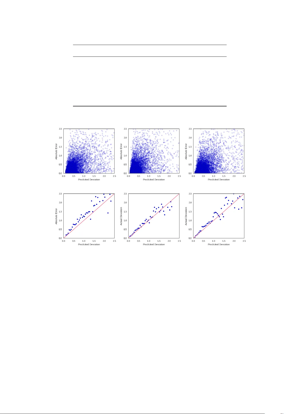
Proceedings of Machine Learning for Healthcare 2017 JMLR W&C Track V olume 68 Pr edicting Surgery Duration with Neural Heter oscedastic Regr ession Nathan H Ng 1 , Rodney A Gabriel 2 , 3 , Julian McA uley 1 , Charles Elkan 1 , Zachary C Lipton 1 , 2 ∗ Department of Computer Science 1 Division of Biomedical Inf ormatics 2 Department of Anesthesiology 3 University of Calif ornia, San Diego 9500 Gilman Drive La J olla, CA 92093, USA {nhng, ragabriel, jmcauley, elkan, zlipton}@ucsd.edu Abstract Scheduling surgeries is a challenging task due to the fundamental uncertainty of the clinical environment, as well as the risks and costs associated with under- and over -booking. W e investig ate neural regression algo- rithms to estimate the parameters of sur gery case durations, focusing on the issue of heter oscedasticity . W e seek to simultaneously estimate the duration of each sur gery , as well as a sur gery-specific notion of our un- certainty about its duration. Estimating this uncertainty can lead to more nuanced and ef fecti ve scheduling strategies, as we are able to schedule surgeries more efficiently while allowing an informed and case-specific margin of error . Using surgery records from a large United States health system we demonstrate potential improv ements on the order of 20% (in terms of minutes o verbooked) compared to current scheduling tech- niques. Moreover , we demonstrate that surgery durations are indeed heteroscedastic. W e show that models that estimate case-specific uncertainty better fit the data (log likelihood). Additionally , we show that the het- eroscedastic predictions can more optimally trade off between over and under-booking minutes, especially when idle minutes and scheduling collisions confer disparate costs. 1. Intr oduction In the United States, healthcare is expensiv e and hospital resources are scarce. Healthcare expenditure now exceeds 17% of US GDP (W orld Bank, 2014), e ven as surgery w ait times appear to ha ve increased o v er the last decade (Bilimoria et al., 2011). One source of inefficiency (among many) is the inability to fully utilize hospital resources. Because doctors cannot accurately predict the duration of sur geries, operating rooms can become congested (when surgeries run long) or lie v acant (when the y run short). Over-booking can lead to long wait times and higher costs of labor (due to ov er -time pay), while under-booking decreases throughput, increasing the marginal cost per sur gery . At present, doctors book rooms according to a simple formula. The default time reserved is simply the mean duration of that specific procedure. The procedure code does in f act e xplain a significant amount of the variance in sur gery durations. But by ignoring other signals, we hypothesize that the medical system lea ves important signals untapped. W e address this issue by developing better and more nuanced strategies for sur gery case prediction. Our work focuses on a collection of surgery logs recorded in Electronic Health Records (EHRs) at a lar ge United States health system. For each patient, we consider a collection of pre-operati ve features, including patient attributes (age, weight, height, sex, co-morbidities, etc.), as well as attrib utes of the clinical en vironment, such as the surgeon, surgery location, and time. For each procedure, we also know ho w much time was originally scheduled, in addition to the actual ‘gr ound-truth’ surgery duration, recorded after each procedure is performed. ∗ . Corresponding author, website: http://zacklipton.com c  2017. W e are particularly interested in de veloping methods that allo w us to better estimate the uncertainty associated with the duration of each surgery . T ypically , neural network regression objectives assume ho- moscedasticity , i.e., constant le vels of target v ariability for all instances. While mathematically conv enient, this assumption is clearly violated in data such as ours: as one might surmise intuiti vely that operations that typically take a long time tend to e xhibit greater v ariance than shorter ones. F or e xample, among the 30 most common procedures, epidur al injections are both the shortest procedures and the ones with the least v ariance (Figure 1). Among the same 30 procedures, exploratory lapar otomy and major burn surg ery exihibit the greatest variance. All procedures e xhibit long (and one-sided) tails. T o model this data, we re visit the idea of heteroscedastic neural re gression, combining it with e xpressi ve, dropout-regularized neural networks. In our approach, we jointly learn all parameters of a predictive distri- bution. In particular, we consider Gaussian and Laplace distributions, each of which is parameterized by a mean and standard de viation. W e also consider Gamma distributions, which are especially suited to surviv al analysis. Unlike the Gaussian and Laplace which are long tailed on both ends, the gamma has a long right tail and has only positiv e support (i.e., it assigns zero probability density to any value less than zero). The restriction to positive v alues suits the modeling of durations or other surviv al-type data. While the gamma distribution (and the related W eib ull distrib ution) has been applied to medical data with classical approaches Bennett (1983); Sahu et al. (1997), this is, to our knowledge, the first to approximate the a parameters of a gamma distribution using modern neural netw ork approaches. Our heteroscedastic models better fit the data (as determined by log likelihood) compared to both current practice and neural network baselines that fail to account for heteroscedasticity . Furthermore, our mod- els produce reliable estimates of the variance, which can be used to schedule intelligently , especially when ov er-booking and under-booking confer disparate costs. These uncertainty estimates come at no cost in per- formance by traditional measures. The best-performing Gamma MLP model achiev es a lower mean squared error than a vanilla least squares (Gaussian) MLP , despite optimizing a dif ferent objective. 2. Dataset Our dataset consists of patient records extracted from the EHR system at a large United States hospital. Specifically , we selected 107,755 records corresponding to sur geries that took place between 2014 and 2016. These sur geries span 995 distinct procedures, and were performed by 368 distinct surgeons. Histograms of both are long-tailed, with over 796 procedures performed fewer than 100 times and 213 doctors performing fewer than 100 surgeries each. Moreov er the data contains sev eral clerical mistakes in logging the durations. For example, a number of sur geries in the record were reported as running less than 5 minutes. Discussions with the hospital experts suggest that this may indicate either clerical errors or an inconsistently applied con vention for logging canceled sur geries. Additionally , sev eral sur geries were reported to run o ver 24 hours, suggesting (rare) clerical errors in logging the end times of procedures. W e remove all surgeries reported to take less than 5 minutes or more than 24 hours from the dataset. This preprocessing left us with roughly 80% of our original data (86,796 examples). F or our experiments, we split this remaining data 80%/8%/12% for training/validation/testing. 2.1 Inputs For each sur gery , we e xtracted a number of pre-operati ve features from the corresponding EHRs. W e restrict attention to features that are available for a majority of patients and (to avoid target leaks) e xclude any information that is charted during or following the procedure. Our features fall into sev eral categories: patient, doctor , procedure, and context. Patient features: For each of our patients, we include the follo wing features: • Size: Patient height and weight are real-v alued features. W e normalize each to mean 0 , v ariance 1 . • Age: A categorical variable, binned according to ten-year wide intervals that are open on the left side (0 − 10] , (10 − 20] , . . . None of the patients in our cohort are zero years old. 2 Figure 1: Distributions of durations for the 30 most common procedures. • ASA score: an ordinal score that represents the sev erity of a patient’ s illness. For example, ASA I denotes a healthy patient, ASA III denotes severe systemic disease, and ASA V denotes that the patient is moribund without surgery . ASA VI refers to a brain-dead patient in preparation for organ transplantation. • Anesthesia T ype: This categorical feature represents the type of anesthesia applied to sedate the patient. The v alues assigned to this variable include General , Monitor ed anesthesia car e (MA C) —in which a patient under goes local anesthesia together with sedation, Neuraxial , No Anesthesiologist , and other/unknown . • Patient Class: This categorical feature indicates the patient’ s current status. The v alues assigned to this variable include Emer gency Department Encounter , Hospital Outpatient Procedur e , Hospital Outpatient Sur gery , Hospital Inpatient Surg ery , T rauma Inpatient Admission , Inpatient Admission , T rauma Outpatient . • Comorbidities: W e model the follo wing co-morbidities as binary v ariables: smoker status, atrial fib- rillation, chronic kidney disease, chronic obstructiv e pulmonary disease, congesti v e heart failure, coro- nary artery disease, diabetes, hypertension, cirrhosis, obstructi v e sleep apnea, cardiac device, dialysis, asthma, and dementia. Doctor: W e represent the doctor performing the procedure (categorical) using a one-hot vector . The doctor feature exhibits considerable class imbalance, with the most prolific doctor performing 3770 surgeries and the least prolific doctor (in the pruned dataset) performing 100 . 3 Featur e Abbr eviation T ype #Categories Mode Age age Categorical 9 50 - 60 Sex sex Binary 2 Female W eight weight Numerical - - Height height Numerical - - Time of Day hour Categorical 8 9:00-12:00 Day of W eek day Cate gorical 7 Friday Month month Categorical 12 March Location location Categorical 10 - Patient Class class Cate gorical 7 Hospital Outpatient ASA Rating asa Categorical 6 None Anesthesia T ype anesthesia Cate gorical 5 General Surgeon surgeon Categorical 155 - Procedur e procedure Categorical 199 Colonoscopy Smoker smoker Binary 2 No Heart Arrhytmia afib Binary 2 No Chronic Kidney Disease ckd Binary 2 No Congestive Heart Failur e chf Binary 2 No Coronoary Artery Disease cad Binary 2 No T ype II Diabetes diabetes Binary 2 No Hypertension htn Binary 2 No Liver Cirrhosis cirrhosis Binary 2 No Sleep Apena osa Binary 2 No Cardiac Device cardiac_de vice Binary 2 No Dialysis dialysis Binary 2 No Asthma asthma Binary 2 No Dementia dementia Binary 2 No Cognitive Impairment cognitiv e Binary 2 No T able 1: Summary of features. Procedur e: W e represent the procedure performed as a one-hot vector . The most common operations tend to be minor GI procedures: the four most frequent procedures are colonoscopy , upper GI endoscopy , catar act r emoval , and abdominal paracentesis . This distribution is also long-tailed with 11,173 colonoscopies. Context: W e represent the conte xt of the procedure with se veral categorical variables. First, we represent the hour of the day as a categorical v ariable with v alues binned into 8 non-overlapping 3 -hour width b uckets. Second, we represent the day of the week and month of the year each as one-hot vectors. Finally , we similarly represent the location of the operations as a one-hot vector . W e summarize the number and kind of features in our dataset in T able 1. W e handle variables with missing values, including height, weight, and hour of the day , by incorporating missing value indicators, following pre vious work on clinical datasets (Lipton et al., 2016). 3. Methods This paper addresses the familiar task of regression. W e start off by refreshing some basic preliminaries. Giv en a set of examples { x i } , and corresponding labels { y i } , we desire a model f that outputs a prediction ˆ y = f ( x ) . The task of the machine learning algorithm is to produce the function f giv en a dataset D consisting of examples X and labels y . Generally , we seek predictions that are somehow close to y , as 4 determined by some computable loss function L . Most often we minimize the squared loss L = P i ( y i − ˆ y i ) 2 for all instances ( x i , y i ). One popular method for producing such a function is to choose a class of functions f parameterized by some v alues θ . Linear models are the simplest examples of this approach. T o train a linear re gression model, we define f ( x ) = θ T x . Then we solve the follo wing optimization problem: θ ∗ = argmin θ L ( y , ˆ y ) ov er some training data and ev aluate the model by its performance on previously unseen data. F or linear models, the error -minimizing parameters (on the training data) can be calculated analytically . For all modern deep learning models, no analytic solution exists, so optimization typically proceeds by stochastic gradient descent. For neural network models, we change only the function f . In multilayer perceptrons (MLP) for example, we transform our input through a series of matrix multiplications, each followed by a nonlinear activ ation function. Formally , an L -layer MLP for regression has the simple form ˆ y = W L · φ ( W L − 1 · . . . · φ ( W 1 · x + b 1 ) + . . . + b L − 1 ) + b L , where φ is an activ ation function such as sigmoid, tanh, or rectified linear unit (ReLU) and θ consists of the full set of parameters W l and b l . W e might view the loss function (squared loss) as simply an intuitiv e measure of distance. Alternatively , it’ s possible to derive the choice of squared loss by viewing re gression from a probabilistic perspectiv e. In the probabilistic view , a parametric model outputs a distribution P ( y | x ) . In the simplest case, we can assume that the prediction ˆ y is the mean of a Gaussian predictive distribution with some variance σ . In this vie w , we can calculate the probability density of an y y given x , and thus can choose our parameters according to the maximum likelihood principle: θ MLE = max θ n Y i =1 1 √ 2 π ˆ σ 2 exp  − ( y i − ˆ y i ) 2 2 ˆ σ 2  = min θ n X i =1  log( ˆ σ i ) + ( y i − ˆ y i ) 2 2 ˆ σ 2  . (1) Assuming constant ˆ σ , this yields a familiar least-squares objecti ve. In this work, we relax the assumption of constant variance (homoscedasticity), predicting both ˆ y ( θ , x ) and ˆ σ ( θ, x ) simultaneously . While we apply the idea to MLPs, it is easily applied to networks of arbitrary architecture. T o predict the standard deviation ˆ σ of the predicti ve distribution, we modify our MLP to ha v e two outputs: The first output has linear acti v ation and we interpret its output as the conditional mean ˆ y . The second output models the conditional variance ˆ σ . T o enforce positivity of ˆ σ , we run this output through the softplus activ ation function softplus ( z ) = log(1 + exp( z )) . W e extend the same idea to Laplace distrib utions, which turn out to better describe the target variability for surgery duration, and are also maximum likelihood estimators when optimizing the Mean Absolute Error (MAE). Mean Absolute Error corresponds to the av erage number of minutes over or underbooked, and is typically the quantity of interest for this type of scheduling task. The Laplace distribution is parameterized by b = √ 2 σ : θ MLE = max n Y i =1 1 2 b exp  −| y i − ˆ y i | b  = min θ n X i =1  log b + | y i − ˆ y i | b  . (2) Finally , we apply the same technique to perform neural re gression with gamma predictiv e distrib utions. The gamma distrib ution has strictly positi ve support and is long-tailed on the right. Since surgeries and other surviv al-type data have nonnegativ e lengths, probability distrib utions with similarly nonnegati ve support such as the gamma distrib ution (compared to the real-valued support of the Gaussian and Laplace distributions), might better describe surgery duration. Formally , the expected time between surgeries (or their associated durations) follows a g amma distribution when sur gery start times are modeled as a Poisson process. 5 The gamma distribution is parametrized by a shape parameter k and a scale parameter Φ : θ MLE = max n Y i =1 1 Γ( k )Φ k y k − 1 i exp  − y i Φ  = min θ n X i =1  log(Γ( k )) + k log Φ − ( k − 1) log y i + y i Φ  . (3) In this case, the model no w needs to predict two values: ˆ k ( θ, x ) and ˆ Φ( θ , x ) . As before, our MLP has two outputs, with both passed through a softplus activ ation to enforce positivity . 4. Experiments W e no w present the basic experimental setup. For all experiments we use the same 80% / 8% / 12% train- ing/validation/test set split. Model weights are updated on the training set and we choose all non-differentiable hyper-parameters and architecture details based on v alidation set performance. In the final tally , we hav e 441 features, the majority of which are sparse and accounted for by the one-hot representations o ver procedures and doctors. W e express our labels (the sur gery durations) as the number of hours that each procedure takes. Baselines W e consider three sensible baselines for comparison. The first is to follow the current heuristic of predicting the a verage time per procedure. Note that this is equiv alent to training an unregularized linear regression model with a single feature per procedure and no others. Although the main technical contrib ution of this paper is concerned with modeling heteroscedasticity , we are also generally interested to know how much performance the current approach lea ves untapped. This baseline helps us to address this question. W e also compare against linear regression. While we tried applying ` 2 regularization, choosing the strength of regularization λ on holdout data, this did not lead to improved performance. Finally , we compare against traditional multilayer perceptrons. T o calculate NLL for models that assume homoscedasticity , we choose the constant variance that minimizes NLL on the v alidation set. T raining Details F or all neural network experiments, we use MLPs with ReLU acti v ations. W e optimize each network’ s parameters by stochastic gradient descent, halving the learning rate ev ery 50 epochs. For each experiment, we used an initial learning rate of . 1 . T o determine the architecture, we performed a grid search ov er the number of hidden layers (in the range 1-3) and ov er the number of hidden nodes, choosing between 128, 256, 384, 512. As determined by our hyper -parameter optimization, for homoscedastic models, all MLPs use 1 hidden layer with 128 nodes. All heteroscedastic models use 1 hidden layer with 256 nodes. All models use dropout regularization. For our basic quantitative ev aluation, we report the root mean squared error (RMSE), mean absolute error (MAE), and ne gati ve log-likelihood (NLL). F or heteroscedastic models, we e valuate NLL using the predicted parameters of the distribution. For the Gamma distrib ution, we calculate its mean as k · Φ . W e use its mean as the prediction ˆ y for calculating RMSE. T o calculate MAE, we use the median of the Gamma distribution as ˆ y . Although the median of a Gamma distribution has no closed form, it can be ef ficiently approximated. W e summarize the results in T able 2. The heteroscedastic Gamma MLP performs best as measured by both RMSE and NLL, while the Laplace MLP performs best as measured by MAE. All heteroscedastic mod- els outperform all homoscedastic models (as determined by NLL) with the heteroscedastic Gamma MLP achieving an NLL of . 4668 as compared to 1 . 062 by the best performing homoscedastic model (Laplace MLP). The significant quantity when ev aluating log likelihood is the differ ence between NLL v alues, corre- sponding to the (log of the) likelihood ratio between two models. Plots in Figure 2 demonstrate that the predicted de viation reliably estimates the observed error , and QQ plots (Figure 3) demonstrate that the Laplace distribution appears to fit our targets better than a Gaussian predictiv e distribution. This giv es some (limited) insight into why the Laplace predictiv e distrib ution might better fit our data than the Gaussian. 6 Models RMSE MAE NLL Change in NLL vs. Current Method Current Method 49 . 80 28 . 87 1 . 2385 0 . 0000 Procedur e Means 49 . 06 27 . 70 1 . 2222 0 . 0164 Linear Regression 45 . 23 25 . 07 1 . 1446 0 . 0939 MLP Gaussian 43 . 51 23 . 90 1 . 1102 0 . 1283 MLP Gaussian HS 44 . 03 24 . 23 0 . 7325 0 . 5060 MLP Laplace 44 . 24 23 . 14 1 . 0621 0 . 1765 MLP Laplace HS 45 . 07 23 . 41 0 . 5034 0 . 7351 MLP Gamma HS 43 . 38 23 . 23 0 . 4668 0 . 7717 T able 2: Performance on test-set data (lower is better). MLP models outperform alternatives at the 1% significance lev el or better . (a) Gaussian (b) Laplacian (c) Gamma (d) Gaussian (e) Laplacian (f) Gamma Figure 2: Plots of predicted ˆ σ against absolute error with heteroscedastic Gaussian (a), Laplacian (b), and Gamma (c) models. A veraging ov er bins of width 0 . 05 (d) (e) (f), sho ws that ˆ σ i is a reliable estimator of the observed error . 5. Related W ork Previous work in in the medical literature addresses the prediction of surgery duration (Eijkemans et al., 2010; Kayı ¸ s et al., 2015; Devi et al., 2012), accounting for both patient and surgical team characteristics. T o our kno wledge ours is the first paper to address the problem with modern deep learning techniques and the first to model its heteroscedasticity . The idea of neural heteroscedastic regression was first proposed by Nix and W eigend (1994), though they do not share hidden layers between the two outputs, and are only concerned with Gaussian predictive distributions. W illiams (1996) use a shared hidden layer and consider the case of multi variate Gaussian distributions, for which the y predict the full cov ariance matrix via its Cholesky factorization. Heteroscedastic regression has a long history outside of neural networks. Le et al. (2005) 7 (a) Gaussian QQ Plot (b) Laplace QQ Plot Figure 3: QQ plots of observed error for Gaussian and Laplace noise models. The Laplace distrib ution better describes observed error , with shorter tails at both ends. address a formulation for Gaussian processes. Most related is Lakshminarayanan et al. (2016) which also revisits heteroscedastic neural re gression, also using a softplus activ ation to enforce non-negati vity . W e sho w some successful modifications to the abov e work, such as the use of the Laplace distrib ution, but our more significant contribution is the application of the idea to clinical medical data. 6. Discussion Our results demonstrate both the efficacy of machine learning (over current approaches) and the heteroscedas- ticity of surgery duration data. In this section, we explore both results in greater detail. Specifically , we analyze the models to see which features are most predictive and examine the uncertainty estimates to see how the y might be used in decision theory to lower costs. 6.1 F eature Importance First, we consider the importance of the various features. Perhaps the most common way to do this is to see which features corresponded to the largest weights in our linear model. These results are summarized in Figure 4. Not surprisingly , the top features are dominated by procedures. In particular pulmonary throm- boendarterectomy recei ves the highest positiv e weight. This procedure in volv es a high risk of mortality , a full cardiopulmonary bypass, hypothermia and full cardiac arrest. Interestingly , ev en after accounting for proce- dures, two doctors recei ve high weight. One (Doctor 266) recei ves significant negativ e weight, indicating unusual ef ficiency and another (Doctor 296) appears to be unusually slow . For ethical reasons, we maintain the anonymity of both the doctors and their specialties. For neural network models, we ev aluate the importance of each feature group by performing an ablation analysis (Figure 5). As a group, procedure codes are ag ain the most important features. Howe ver , location, patient class, surgeon, anesthesia, and patient sex all contribute significantly . The hour of day appears to influence the performance of our models b ut the day of the week does not and the month appears to merely introduce noise, leading to a reduction in test set performance. Interestingly , comorbidities also made little difference in performance. Howe ver , it is possible that these features only apply to a small subset of patients but are highly predicti ve for that subset. 6.2 Economic Analysis Our aim in predicting the variance of the error is to provide uncertainty information that could be used to make better scheduling decisions. T o compare the v arious approaches from an economic/decision-theoretic 8 Figure 4: T op 30 linear regression features sorted by coef ficient magnitude. perspectiv e, we might consider the plausible case where the cost to over -reserve the room by one minute (pro- cedure finishes early) dif fers from the cost to under -reserve the room (procedure runs o v er). W e demonstrate how the tw o quantities can be traded of f in Figure 6. For models that don’t output variance, we consider scheduled durations of the form ˆ y + k and ˆ y · k where k is a data-independent constant. In either case, by modulating k , one books more or less aggressively . The multiplicativ e approach performed better, likely because long procedures have higher variance than short ones. This approach is equiv alent to selecting a certain percentile of each predicted distribution giv en a constant sigma. For heteroscedastic models we make the trade-off by selecting a constant percentile of each predicted distribution. When the cost of o ver -reserving by one minute and under-reserving by one minute are equal, the problem reduces to minimizing absolute error . Around this point on the curve the homoscedastic Laplacian outperforms all other models. Ho wever , giv en cost sensiti vity , the heteroscedastic Gamma strictly outper- forms all other models. 6.3 Future W ork W e are encouraged by the efficacy of simple machine learning methods both to predict the durations of surgeries and to estimate our uncertainty . W e see several promising a venues for future work. Most concretely , we are currently engaged in discussions with the medical institution whose data we used about introducing a trial in which surgeries would be scheduled according to decision theory based on our estimates. Regarding methodology , we look forward to expanding this research in sev eral directions. First, we might extend the approach to modeling covariances and more complex interactions among multiple real-valued predictions. W e might also consider problems like bounding box detection, requiring more complex neural architectures. References Stev e Bennett. Log-logistic regression models for surviv al data. Applied Statistics , pages 165–171, 1983. Karl Y Bilimoria, Clifford Y Ko, James S T omlinson, Andrew K Ste wart, Mark S T alamonti, Denise L Hynes, David P W inchester, and Da vid J Bentrem. W ait times for cancer surgery in the united states: trends and predictors of delays. Annals of sur gery , 253(4):779–785, 2011. 9 Figure 5: Ablation analysis of feature importance for neural models. S Prasanna Devi, K Suryaprakasa Rao, and S Sai Sangeetha. Prediction of sur gery times and scheduling of operation theaters in optholmology department. J ournal of medical systems , 2012. Marinus JC Eijkemans, Mark van Houdenhoven, Tien Nguyen, Eric Boersma, Ewout W Steyerber g, and Geert Kazemier . Predicting the unpredictable: A new prediction model for operating room times using individual characteristics and the surgeon’ s estimate. The J ournal of the American Society of Anesthesiol- ogists , 2010. Enis Kayı¸ s, T aghi T Khaniye v , Jaap Suermondt, and Karl Sylv ester . A rob ust estimation model for surgery durations with temporal, operational, and surgery team ef fects. Health care management science , 2015. Balaji Lakshminarayanan, Alexander Pritzel, and Charles Blundell. Simple and scalable predictiv e uncer- tainty estimation using deep ensembles. arXiv pr eprint arXiv:1612.01474 , 2016. Quoc V Le, Ale x J Smola, and Stéphane Canu. Heteroscedastic gaussian process re gression. In ICML , 2005. Zachary C Lipton, David C Kale, and Randall W etzel. Modeling missing data in clinical time series with rnns. In Machine Learning for Healthcare , 2016. David A Nix and Andreas S W eigend. Estimating the mean and v ariance of the tar get probability distrib ution. In International Confer ence on Neural Networks . IEEE, 1994. 10 Figure 6: T otal ov er-booking and under-booking errors for different models as we adjust predicted values. Predictions were selected by considering different percentiles of the distrib ution predicted for each case. For homoscedastic models, this was equi v alent to multiplying each prediction by a constant v alue. Sujit K Sahu, Dipak K Dey , Helen Aslanidou, and Debajyoti Sinha. A weib ull re gression model with gamma frailties for multiv ariate surviv al data. Lifetime data analysis , 3(2):123–137, 1997. Peter M W illiams. Using neural networks to model conditional multi v ariate densities. Neur al Computation , 1996. W orld Bank. Health e xpenditure, total (% of gdp), 2014. URL http://data.worldbank.org/ indicator/SH.XPD.TOTL.ZS . 11