Bayesian Lower Bounds for Dense or Sparse (Outlier) Noise in the RMT Framework

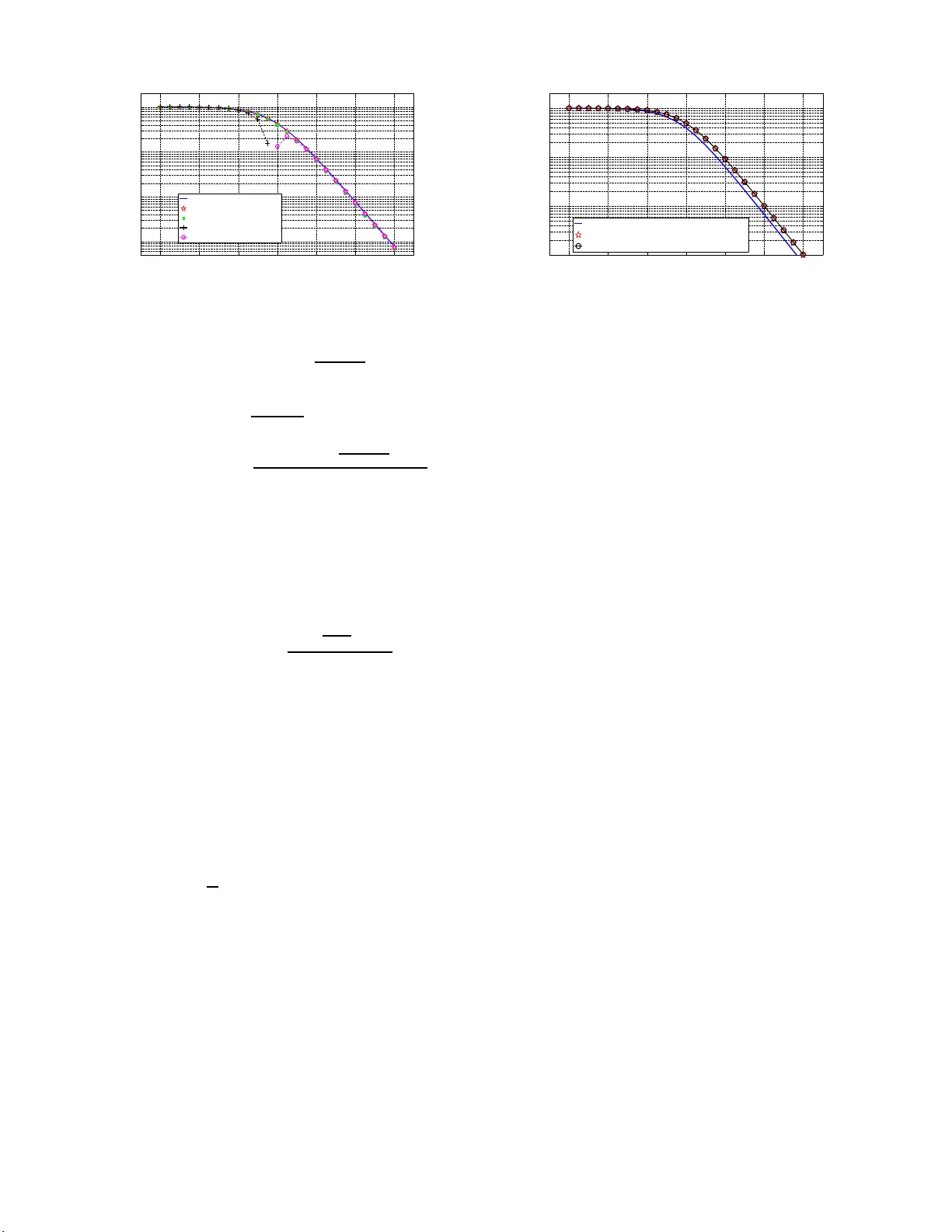
Bayesian Lo wer Bounds for Dense or Sparse (Outlier) Noise in the RMT Frame w o rk V ir ginie Ollier ∗ † , R ´ emy Bo yer † , Mohammed Nabil El K orso ‡ and Pasc al Larzabal ∗ ∗ SA TIE, UMR 8029, Un iversit ´ e Paris-Saclay , ENS Cachan , Cachan, Franc e † L2S, UMR 850 6, Universit ´ e Paris-Saclay , Universit ´ e Paris-Sud, Gif-su r-Yvette, France ‡ LEME, EA 4416, Universit ´ e Paris-Ouest, V ille d’A vray , Franc e Abstract —Robust estimation is an important and timely re- search su bject. In t his paper , we in vestigate perfo rmance lower bounds on the mean-square-error (MSE ) of any estimator fo r the Bayesian linear model, corrupted by a noise di stri buted according to an i.i.d . Student’ s t-distribution. This class of prior parametrized by its d egree of freedom is releva nt to modelize either dense or sparse (accounting for outl iers) noise. Using the hierarchical Normal-Gamma representation of the Student’s t-d i stribution, the V an T rees’ Bayesian Cram ´ er -Rao bound (BCRB) on the amplitud e parameters is derived. Further - more, the random matrix theory (RMT ) framework is assumed, i.e. , the number of measurements and t he number of unknown parameters gro w joint ly to infin ity with an asymptotic fi nite ratio. Using some powerful res ults from the RMT , closed-f orm expressions of the BCRB are derived and studied. Finally , we propose a framework to fairly compare two models corrupted by noises with diff erent degrees of freedom f or a fixed common target signal-to-n oise ratio (SNR). In particular , we focus our effo rt on the comparison of the BCRB s associated with two models corrupted by a sparse noise p romoting outl iers and a dense (Gaussian) noise, respectively . Index T erms —Bayesian hierarchical linear model, Bayesian Cram ´ er -Rao boun d, sparse outlier noise, den se noise, random matrix theory I . I N T RO D U C T I O N In the context of r obust data mod eling [1], th e measure- ment vector may be corrup ted by no ise contain ing outliers. This c lass of noise is sometimes referred to as sparse noise and is described by a distribution with h eavy-tails [2]–[ 7]. Con versely , we usually call den se a noise th at does n ot share this pr operty and the m ost po pular prior is probably Gau ssian noise. Depend ing on the app lica tio n con text, outliers may be identified, e.g. , as co rrupted inf ormation or incomp lete data [8]. A robust and relevant n oise prio r which is a b le to take into accoun t outliers is th e Stu d ent’ s t- d istribution with low degrees of fre e dom [9]–[1 2]. In add itio n, dense noise can also be encompassed thanks to the Student’ s t-distribution prio r for an infinite degree o f freedom . A convenient framework to deal with a wid e class of distributions is well known under the nam e of h ierarchical Bayesian modeling . The Bayesian hierarchica l linear mo del (BHLM) with hierarchical n oise prior is used in a wide r a nge of applications, including fusion This work was supported by the follo wing projec ts: MAGELLAN (ANR- 14-CE23-0004-0 1) and ICode blanc. [13], anoma ly detection of h y perspectra l imag es [5], chann el estimation [1 4], blind deconv o lu tion [1 5], segmentation o f astronomica l times series [16], etc . In this work, we ad opt suc h hierar chical prior framework due to its flexibility and ability to mode lize a wide class of priors. More p recisely , the n oise vector is assumed to follow a circular i.i. d. center ed Gaussian p rior with a variance de fin ed by the in verse of an unk nown r andom hyp e r-parameter . I n addition, if this hy p er-parameter is Gam ma distributed [17,18], then the marginalized join t pd f over the hyper-parame te r is the Student’ s t-distribution. The V an Trees’ Bayesian Cram ´ er-Rao bo und ( BCRB ) [1 9] is a stan dard and fundam e ntal lower boun d on the mean- square-er r or ( MSE ) of any estimator . The aim o f this work is to d erive an d analy z e the BCRB of th e am p litude pa rameters ( i ) for the consider ed noise prior and ( ii ) using some powerful results from the rando m matrix theory (RMT) fra m ew o rk [20]– [22]. Regarding refer ence [23], the proposed work is origin al in the sen se that the noise p rior is d ifferent and the asym p totic regime is assumed. Finally , note that reference [ 24] tack les a similar p roblem but does n ot assume the asymp to tic context. W e use the following n o tation. Scalars, vectors and ma- trices a r e den oted b y italic lower -case, boldface lower - case and boldface upp er-case symbols, respectively . The symbol T r[ · ] stand s for the trace ope rator . Th e K × K identity matrix is den oted by I K and 0 K × 1 is the K × 1 vector filled with zeros. The pro bability density function (pdf) of a g i ven rand om variable u is denoted b y p ( u ) . Th e sym- bol N ( · , · ) refers to the Gaussian distribution, para metrized by its mean and covariance matrix, G ( · , · ) is th e Gamma distribution, described b y its shape and rate (in verse scale) parameters, while I G ( · , · ) is the inverse-Gamma distribution. If we have u ∼ G ( a, b ) then p ( u | a, b ) = b a u a − 1 e − bu Γ( a ) , where Γ( · ) is the Gamma f unction. An d if u ∼ I G ( a, b ) , th en p ( u | a, b ) = b a u − a − 1 e − b u Γ( a ) . The n on-stand a r dized Stu dent’ s t- distribution is define d by thre e p arameters, through the pdf p ( u | µ, σ 2 , ν, ) = Γ( ν +1 2 ) Γ( ν 2 ) √ π ν σ 2 (1 + 1 ν ( u − µ ) 2 σ 2 ) − ν +1 2 such that u ∼ S ( µ, σ 2 , ν ) . As regards the b iv ariate Norm al-Gamma distribution, if we have ( u , w ) ∼ No rmalGamma( µ, λ, a , b) , then p ( u, w | µ, λ, a, b ) = b a √ λ Γ( a ) √ 2 π w a − 1 2 e − bw e − λw ( u − µ ) 2 2 . Fi- nally , the symbol a.s. → deno tes a lmost su r e conver gence, O ( · ) is th e b ig O no tatio n, λ i ( · ) is the i -th eigenv alue of the con - sidered matrix and the symbo l E u | w refers to the expectation with r e spect to p ( u | w ) . I I . B AY E S I A N L I N E A R M O D E L C O R RU P T E D B Y N O I S E O U T L I E R S A. Definition of the random mo d el Let y b e th e N × 1 vector o f measur ements. The BHLM is defined b y y = Ax + e , (1) where each elemen t [ A ] i,j of the N × K matrix A , with K < N , is d rawn fr om an i.i.d . as a single realization of a sub- Gaussian distribution with zero-mean and variance 1 / N [22, 25]. T he unk nown amp litude vector is gi ven by x = [ x 1 , . . . , x K ] T ∼ N ( 0 K × 1 , σ 2 x I K ) , (2) where σ 2 x is the kn own am plitude variance. In additio n, the measuremen ts are con taminated by a noise vector e which is assumed statistically independ ent from x . B. Hierar chical Normal-Gamma r epr esentation The i - th n oise sample is assumed to be circu lar centered i.i.d. Gau ssian according to e i | γ ∼ N  0 , σ 2 γ  , (3) where γ σ 2 is usually called the no ise precision , γ is an unkn own hyper-parameter and σ 2 is a fixed scale parameter . If the hyper-parame ter is Gam ma distributed accord in g to γ ∼ G  ν 2 , ν 2  , (4) where ν is the numb er of degrees of freedo m, the jo int distribution of ( e i , γ ) f ollows a No rmal-Gamm a distribution [26] such as ( e i , γ ) ∼ NormalGamma  0 , 1 σ 2 , ν 2 , ν 2  . (5) The marginal distribution of the joint p df over the h yper- parameter γ leads to a non-standard ized Student’ s t- distribution, giv e n by [11,2 7] S ( e i | 0 , σ 2 , ν ) = Z ∞ 0 N  e i | 0 , σ 2 γ  G  γ | ν 2 , ν 2  d γ , (6) such that e i ∼ S (0 , σ 2 , ν ) . As ν → ∞ , the d istribution ten ds to a Gaussian with zero - mean and variance σ 2 , while it b ecomes more h eavy-tailed when ν is small [12,2 8]. W ith (3) and ( 4), and knowing that 1 γ ∼ I G ( ν 2 , ν 2 ) , we notice that th e variance, no ted σ 2 e of each noise entry of e , is given by th e following expression σ 2 e = E γ E e i | γ  e 2 i  = σ 2 E γ  1 γ  = σ 2 ν ν − 2 , (7) in wh ich ν > 2 . I I I . BCRB F O R S T U D E N T ’ S T - D I S T R I B U T I O N The vector of unknown par ameters, denoted by θ , en com- passes th e amplitude vector and the noise hy per-parameter, i.e. , θ = [ x T , γ ] T . (8) Giv en a n indep endenc e assump tion between x and γ , the joint pdf p ( y , θ ) can be decomp osed as p ( y , θ ) = p ( y | θ ) p ( θ ) = p ( y | θ ) p ( x ) p ( γ ) . (9) Let us note ˆ θ an e stimator of the unknown vecto r θ . Then, the mean squar e error ( MSE ), direc tly linked to the error covariance matrix , verifies the following inequality MSE( θ ) = T r h E y , θ n ( θ − ˆ θ )( θ − ˆ θ ) T oi ≥ T r [ C ] , (10 ) where C is the ( K + 1) × ( K + 1) BCRB matrix defined as the inverse of th e Bayesian Info rmation Matrix (BIM) J . W e can show that the BIM has a block -diagon al struc ture du e to the indep endence between parameters. Thu s, we write J =  J x , x 0 K × 1 0 1 × K J γ , γ  . (11) W e assume an identifiable BHLM mod el so that, un der weak regularity conditions [19], the BIM is given by J = E θ n J ( θ , θ ) D o + J ( θ , θ ) P + J ( θ , θ ) H P , (12) in which [ J ( θ , θ ) D ] i,j = E y | θ  − ∂ 2 log p ( y | θ ) ∂ θ i ∂ θ j  , (13) [ J ( θ , θ ) P ] i,j = E x  − ∂ 2 log p ( x ) ∂ θ i ∂ θ j  , (14) [ J ( θ , θ ) H P ] i,j = E γ  − ∂ 2 log p ( γ ) ∂ θ i ∂ θ j  (15) for ( i, j ) ∈ { 1 , . . . , K + 1 } 2 , and where J ( θ , θ ) D is the Fisher Inform ation Matr ix ( FIM) on θ , J ( θ , θ ) P is th e p rior pa rt o f the BIM an d J ( θ , θ ) H P is the hyper-prior part. Correspon d ingly , we hav e C = J − 1 =  C x , x 0 K × 1 0 1 × K C γ , γ  . (16) Conditionally to θ , the ob servation vector y has th e f o llow- ing Gaussian distribution y | θ ∼ N  µ , R  , (17 ) where µ = Ax and R = ( ν − 2) σ 2 e ν γ I N . In what fo llows, we directly make use of the Slepian-Ban gs formula [29, p. 37 8] [ J ( θ , θ ) D ] i,j =  ∂ µ ∂ θ i  T R − 1 ∂ µ ∂ θ j + 1 2 T r  R ∂ θ i R − 1 R ∂ θ j R − 1  . (18) This leads to J ( x , x ) D = ν γ ( ν − 2) σ 2 e A T A . (19) Using the fact that R − 1 = γ σ 2 I N , we obtain J ( γ , γ ) D = σ 4 2 γ 4 T r h R − 2 i = N 2 γ 2 . (20) According to (2) and c o nsidering indep endent amp litu des, we have − log p ( x ) = K X i =1  1 2 log(2 π σ 2 x ) + x 2 i 2 σ 2 x  . (21) Consequently , J ( x , x ) P = 1 σ 2 x I K . (22) The BIM J is therefo re composed of the following terms: J x , x = E γ n J ( x , x ) D o + J ( x , x ) P , (23) J γ , γ = E γ n J ( γ , γ ) D o + J ( γ , γ ) H P . (24) The hy per-prior par t of the BIM is given by J ( γ , γ ) H P = E γ  − ∂ 2 log p ( γ ) ∂ γ 2  = ν − 2 2 E γ  1 γ 2  . (25) The second -order momen t o f an in verse-Gamm a d istributed random variable is giv en by E γ  1 γ 2  = ν 2 ( ν − 2)( ν − 4) , (26) where ν > 4 . This finally leads to J γ , γ = N ν 2 2( ν − 2)( ν − 4) + ν 2 2( ν − 4) . (27) In verting the BIM, we obtain th e BCRB for the amplitude parameters BCRB( x ) = T r [ C x , x ] K with C x , x = σ 2 x  r A T A + I K  − 1 , (28) where r = SNR ν ν − 2 with SNR = σ 2 x σ 2 e (signal-to- n oise ratio). I V . BCRB I N T H E A S Y M P T OT I C F R A M E W O R K A. RMT framework In th is section, we con sider the co ntext o f large random matrices, i.e. , f or K, N → ∞ with K N → β ∈ (0 , 1) . The derived BCRB in th is context is the asym ptotic no rmalized BCRB d efined by BCRB( x ) a.s. → BCRB ∞ ( x ) . (29) Using (28) with [21, p. 11 ], we obtain BCRB ∞ ( x ) = σ 2 x  1 − f ( r , β ) 4 rβ  (30) and f ( r, β ) =  p r (1 + √ β ) 2 + 1 − p r (1 − √ β ) 2 + 1  2 . B. Limit an alytical expr essions • For β ≪ 1 , i.e. , K ≪ N , after some man ipulations and discarding the terms o f o rder sup erior o r equal to O ( β 2 ) , we o b tain f ( r , β ) ≈ 4 β r 2 r + 1 . (31) Therefo re, an asy m ptotic analytical expression of the BCRB , in the RMT framework, is given by BCRB ∞ ( x ) ≈ σ 2 x r + 1 = ( ν − 2) σ 2 x ν (1 + SNR) − 2 . (32) • For small r , also meaning small SNR , accord ing to th e Neu mann ser ies e x pansion [3 0], we hav e  r A T A + I K  − 1 ≈ I K − r A T A if the max imal eigen- value λ max ( r A T A ) < 1 . Observe th at r λ max ( A T A ) a.s. → r (1 + √ β ) 2 [20]–[22]. In addition, if SNR is sufficiently small with respect to ( ν − 2) / (4 ν ) then BCRB( x ) ≈ σ 2 x K  T r [ I K ] − r T r  A T A  a.s. → σ 2 x (1 − r ) = σ 2 x ν − 2 ( ν − 2 − ν SNR) . (33) • For large r , also meaning large SNR , we have BCRB( x ) ≈ σ 2 x rK  T r h  A T A  − 1 i − 1 r T r h  A T A  − 2 i  a.s. → σ 2 x r  1 1 − β − 1 r 1 (1 − β ) 3  = ( ν − 2) σ 2 x ν SNR(1 − β )  1 − ν − 2 ν SNR(1 − β ) 2  , (34) since [20]–[ 22] 1 K T r h  A T A  − 1 i a.s. → 1 1 − β , (35) 1 K T r h  A T A  − 2 i a.s. → 1 (1 − β ) 3 . (36) C. Comparison between two mod els with a tar get com mo n SNR W e consider two different models: ( M 0 ) : y 0 = Ax + e 0 with e i 0 ∼ S (0 , σ 2 0 , ν 0 ) , (37) ( M 1 ) : y 1 = Ax + e 1 with e i 1 ∼ S (0 , σ 2 1 , ν 1 ) . (38) Model ( M 0 ) is the ref e r ence mo del and mode l ( M 1 ) is the alternative one . Acco rding to (30), the asym ptotic no rmalized BCRB f or the k - th mod el with k ∈ { 0 , 1 } is defin e d by BCRB ∞ k ( x ) = σ 2 x  1 − f ( r k , β ) 4 r k β  (39) where r k = SNR k ν k ν k − 2 with SNR k = σ 2 x σ 2 e k . A fair method ol- ogy to comp are the bound s BCRB 0 ( x ) and BCRB 1 ( x ) is to impose a co mmon target SNR for the models ( M 0 ) and ( M 1 ) , i.e. , SNR 0 = SNR 1 . A simple deriv ation shows that to reach −30 −20 −10 0 10 20 30 10 −3 10 −2 10 −1 10 0 SN R (d B ) MS E B CR B ( x ) , wi t h (2 8) B CR B ∞ ( x ) B CR B ∞ ( x ) l ow β B CR B ∞ ( x ) f or s ma l l SN R B CR B ∞ ( x ) f or l ar g e SN R Fig. 1. BCRB ( x ) as a function of SNR in dB with s pecific limit approxi- mations, in the RMT framew ork. the target SNR , we must h av e r 1 = ν 1 ( ν 0 − 2) ν 0 ( ν 1 − 2) r 0 . Specifically , the c o rrespon ding BCRB s are the following ones: BCRB ∞ 0 ( x ) = σ 2 x  1 − f ( r 0 , β ) 4 r 0 β  , (40) BCRB ∞ 1 ( x ) = σ 2 x   1 − ν 0 ( ν 1 − 2) f ( ν 1 ( ν 0 − 2) ν 0 ( ν 1 − 2) r 0 , β ) 4 ν 1 ( ν 0 − 2) r 0 β   . (41) Recall that the Stud ent’ s t-distribution is well known to promo te noise outliers thank s to its heavy-tails prope r ty unlike the Gaussian distribution. So, an interesting scenario arises when ν 1 → ∞ . In this case, the Stud e nt’ s t-distribution conv e rges to the Gaussian on e [10] and (41) ten d s to BCRB ∞ 1 ( x ) ν 1 →∞ = σ 2 x   1 − ν 0 f  ν 0 − 2 ν 0 r 0 , β  4( ν 0 − 2) r 0 β   . (42) D. Numerical simula tions In the following simu lations, we consider N = 100 and K = 1 0 so that β ≪ 1 . T he amplitude variance σ 2 x is fixed to 1 . In Fig. 1, we p lot the B C RB of th e amplitude vecto r x , as defin ed b y equ a tio ns (2 8) and (30) (asympto tic expression), (32) (small β ), (33) (small SNR ) an d ( 34) ( large SNR ), as a function o f the SNR in dB fo r ν = 6 . W e notice that BCRB( x ) coincide s precisely with its asymptotic expression in (30). Th us, the RMT fram ew o rk predicts precisely the behavior of the BCRB of th e amplitud e as K , N → ∞ with K N → β and allows us to o btain a closed- form expression. Such limit remain s co rrect even for values of N and K tha t are relati vely not quite large. The expression o f the B CRB obtained with (32) is a goo d app roximation since here, we have β = 0 . 1 ≪ 1 . Fina lly , we notice tha t the curves obtained for low and high SNR ap p roximate very well the BCRB o f the amplitude, asympto tica lly . In Fig. 2 , as exposed in section IV -C, we con sider two different m odels, with a different value for the number of degrees o f freedo m ν . W e n o tice th at a lower perform ance bound is achieved with ν 0 = 6 , especially in th e low n oise regime, than with ν 1 = 100 . Furtherm ore, the approx im ation in (42) is cor rect, since ν 1 has a large value. A low value −30 −20 −10 0 10 20 30 10 −3 10 −2 10 −1 10 0 MS E ta r ge t com m on SN R i n d B BC R B ∞ 0 ( x ) wi th ν 0 = 6 BC R B ∞ 1 ( x ) wi th ν 1 = 1 00 An al yt i c e xp r e s s io n ( 44 ) for B C R B ∞ 1 ( x ) Fig. 2. Asymptotic normalized BCRBs for models ( M 0 ) and ( M 1 ) vs. a common SNR for th e n umber of degrees o f freedom is well-adapted for the mod elization o f sparse (ou tlier) noise, characte r ized by a heavy-tailed distribution [31,32]. This large level in h eavy- tailedness leads to r o bustness [1,33,34] while a Gaussian noise mo d el ( la rge degre e o f freedom ) corr esponds to a den se noise type. Thus, we can h ope to achieve be tter estimation perfor mances if we con sider a model, which promo tes sparsity and the presence o f outliers in data. V . C O N C L U S I O N This work discu sses fun damental Bayesian lower bound s for m ulti-param eter robust estimation. More precisely , we consider a Bayesian linear mod el corrupted by a sparse n oise following a Student’ s t- distribution. Th is class of p r ior can efficiently m odelize o utliers. Using the hierarc h ical Normal- Gamma represen tation of the Student’ s t-distribution, the V an T re e s’ Bay esian lower b ound ( BCRB ) is de r iv ed for u nknown amplitude parameters in an asymptotic c o ntext. By asymptotic, it means that the nu mber o f measur ements and the number of unknown parame ters g r ow to infinity at a finite rate. Conse- quently , closed-fo rm expressions of the BCRB are ob tained using so m e po werful results fro m the large ran dom matr ix theory . Finally , a fr amew ork is provid ed to fairly com pare two models co rrupted b y noises with different degrees of fr e edom for a fixed common target SNR . W e reca ll that a small degree of freedo m p romotes outliers in the sense that the no ise prior has heavy-tails. For th e am plitude, a lower perform ance b ound is achieved whe n the num ber of degrees of f reedom is small. R E F E R E N C E S [1] A. M. Z oubir , V . Koi vunen, Y . Chakhchoukh, and M. Muma, “Rob ust estimati on in signa l processing: A tutorial-style treatment of fundamenta l concep ts, ” IE EE Signal Pr ocessing Ma gazine , vol. 29, no. 4, pp. 61–80, 2012. [2] K. Mitra, A. V eeraragha v an, and R. Chella ppa, “Rob ust R VM regre s sion using sparse outlier m odel, ” in IEEE Confer ence on Computer V ision and P attern Recogni tion (CVPR) , San Francisco, CA, 2010, pp. 1887– 1894. [3] ——, “Robust regression using sparse learning for high dimensiona l paramete r estimation problems, ” in IEEE Int. Conf. Acoust., Speec h and Signal Proc essing (ICASSP) , Dallas, TX, 2010, pp. 3846–3849. [4] P . Zhuang, W . W ang, D. Z eng, and X. Ding, “Robust mixed noise remov al with non-parametri c Bayesian sparse outlier model, ” in 16th Internati onal W orkshop on Multimedi a Signal P r ocessing (MMSP) , Jakarta , Indonesia, 2014, pp. 1–5. [5] G. E. Newstadt , A. O. Hero, and J. Simmons, “Robust spect ral un- mixing for anomaly detection. ” in IEEE W orkshop on Statistica l Signal Pr ocessing (SSP) , Gold Coast, VIC, 2014, pp. 109–112. [6] M. Sundin, S. Chatterje e, and M. Jansson, “Combined m odeling of sparse and dense noise improv es Bayesian R VM, ” in 22nd Eur opean Signal Proc essing Confer ence (EUSIPCO) , L isbon, Portugal, 2014, pp. 1841–1845. [7] ——, “Bayesia n learni ng for robust Princip al Component Analysis, ” in 23r d Eur opean Signal Pr ocessing Confer ence (EUSIPCO) , Nice, France, 2015, pp. 2361–2365. [8] J. Luttinen, A. Ilin, and J. Karhunen, “Bayesian robust PCA of incom- plete data, ” Neural Pr ocessing Letters , vol. 36, no. 2, pp. 189–202, 2012. [9] D. Peel and G. J. McLachlan, “Robust mixture modelling using the t distributio n, ” Statisti cs and computing , vol. 10, no. 4, pp. 339–348, 2000. [10] S. Kotz and S. Nadarajah, Multi variate t-dist ribut ions and their appli- cations . Cambridge Uni versi ty Press, 2004. [11] J. Christmas, “Baye sian spectra l analysi s with Student-t noise, ” IEEE T ransacti ons on Sign al Pr ocessing , vol . 62, no. 11, pp. 2871–28 78, 2014. [12] H. Zhang, Q. M. J. W u, T . M. Nguyen, and X. Sun, “Syntheti c aperture radar image segmentat ion by modified Student ’ s t-mixture model, ” IEEE T ransacti ons on Geoscie nce and Remote Sensing , vol. 52, no. 7, pp. 4391–4403, 2014. [13] Q. W ei, N. Dobige on, and J .-Y . T ourneret, “Bayesian fusion of hyper- spectra l and multispect ral images, ” in IEEE Int. Conf. on Acoust., Speec h and Signal Proce s sing (ICASSP) , Florence, Italy , 2014, pp. 3176–3180. [14] N. L . Pedersen, C. N. Manch ´ on, D. Shutin, and B. H. Fleury , “ Appli- catio n of Bayesi an hierarchica l prior modelin g to sparse channel esti- mation, ” in IEEE Internationa l Confer ence on Communicati ons (ICC) , Otta wa, ON, 2012, pp. 3487–3492. [15] G. Kail, J.-Y . T ourneret, F . Hlawatsc h, and N. Dobigeon, “Blind decon- volu tion of sparse pulse sequenc es under a m inimum dista nce constraint: A partially collapsed Gibbs sampler method, ” IEEE T ransacti ons on Signal Proc essing , vol. 60, no. 6, pp. 2727–2743, 2012. [16] N. Dobigeon, J.-Y . T ourneret, and J. D. Scar gle, “Joint segmenta tion of multi va riate astronomic al time s eries: Bayesia n sampling with a hierarc hical model, ” IEEE T ransactions on Signal Proc essing , vol . 55, no. 2, pp. 414–423, 2007. [17] A. Gelman, “Prior distrib utions for varianc e parameters in hierar chica l models (comment on arti cle by Bro wne and D raper), ” Bayesian Analysi s , vol. 1, no. 3, pp. 515–534, 2006. [18] J. Dahlin, F . Lindsten, T . B. Sch ¨ on, and A. W ills, “Hierarchica l Bayesian ARX m odels for robust inference , ” in 16th IF AC Symposium on System Identifi cation (SYSID) , Brussels, Belgium, 2012, pp. 131–136. [19] H. L. V an Tre es and K. L. Bell, Bayesian bounds for paramete r estimati on and nonline ar filteri ng/track ing . Ne w Y ork: W iley-IEEE Press, 2007. [20] J. W . Silverstei n and Z . Bai, “On the empirical distribution of eige n- v alues of a class of large dimensiona l random matrice s, ” Journa l of Multiv ariate analysis , vol. 54, no. 2, pp. 175–192, 1995. [21] A. M. Tulino and S. V erd ´ u, Random matrix theory and wirele s s communica tions . Foundations and Trends in Communicatio ns and Information Theory . Now Publishers Inc., 2004, vol. 1, no. 1. [22] R. Couillet and M. Debbah, Random matrix methods for wir eless communica tions . Cambridge Uni versity Press, 2011. [23] M. N. El Korso, R. Bo yer, P . Larzaba l, and B.-H. Fleury , “Estimation performanc e for the Bayesian hierarc hical line ar model, ” IEEE Signal Pr ocessing Letters , vol. 23, no. 4, pp. 488–492, 2016. [24] R. Prasad and C. R. Murthy , “Cram ´ er-Ra o-type bounds for sparse Bayesia n learnin g, ” IE EE T ransact ions on Signal Proce ssing , vol. 61, no. 3, pp. 622–632, 2013. [25] V . V . Buldygin and Y . V . Koza chenko, Metric c haract erization of random variable s and random proc esses . America n Mathemat ical Soc., 2000, vol. 188. [26] J. M. Bernardo and A. F . M. Smith, Bayesian theory . New Y ork: J. W iley , 1994. [27] M. Svens ´ en and C. M. Bishop, “Rob ust Bayesian mixture modell ing, ” Neur ocomputing , vol. 64, pp. 235–252, 2005. [28] G. Sfikas, C. Nikou, and N . Galatsa nos, “Rob ust image segmentat ion with mixtures of Student’ s t-distri butions, ” in International Confer ence on Image Proc essing (ICIP) , vol. 1, Sant Antonio, TX, 2007, pp. I–273 – I–276. [29] P . Stoica and R. L. Moses, Spec tral analysis of signals . Pearson Prent ice Hall, Upper Saddle Riv er , NJ, 2005. [30] G. B. Arfken and H. J. W eber , Mathematical methods for physic ists, sixth edition . Academic press, 2005. [31] G. T zagkara kis and P . Tsakalide s, “Bayesian compressed sensing of a highly impulsiv e signal in hea vy-tailed noise using a multiv ariate Cauchy prior , ” in 17th E ur opean Signal P r ocessing Confer ence , Glasgow , S cot- land, 2009, pp. 2293–2297. [32] A. Amini, M. Unser , and F . Marv asti, “Compressibilit y of deterministi c and random infinite sequences, ” IEEE Tr ansactions on Signal P rocess- ing , vol. 59, no. 11, pp. 5193–5201, 2011. [33] K. L. Lange, R. J. A. Little , and J. M. G. T aylor , “Robust statistica l modeling using the t distribut ion, ” J ournal of the American Statistical Association , vol. 84, no. 408, pp. 881–896, 1989. [34] N. Delanna y , C. Archambea u, and M. V erleysen , “Improving the ro- bustne s s to outlie rs of mixtures of probabilistic PCAs, ” Advance s in Knowled ge Discovery and Data Mining , vol. 5012, pp. 527–535, 2008.