Reinforcement Learning of POMDPs using Spectral Methods

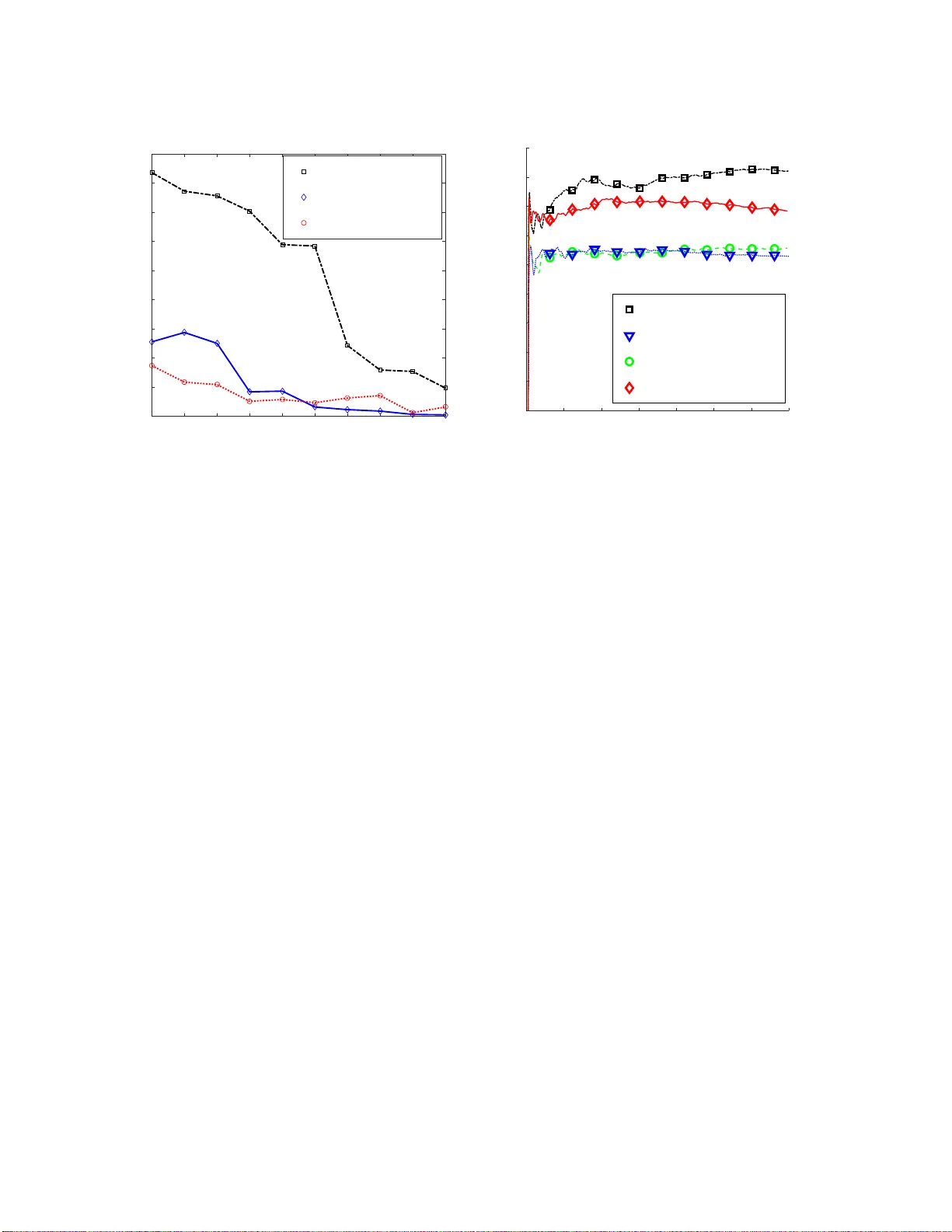
JMLR: W orkshop and Confe rence Proceedings vol 49: 1 – 64 , 2016 Reinf orcement Learn ing of POMDPs using Spectral Methods Kamyar Azizzadenesheli ∗ K A Z I Z Z A D @ U C I . E D U University of California, Irvine Alessandr o Lazaric † A L E S S A N D RO . L A Z A R I C @ I N R IA . F R Institut National de Recher che en Informatique et en A uto matique, (Inria) Animashre e Anand kumar ‡ A . A N A N D K U M A R @ U C I . E D U University of California, Irvine Abstract W e pr opose a new reinforce ment learning algorithm for par ti ally observable Markov decision pro- cesses (POMDP) based on spectral decomposition methods. While spectral methods ha ve been previously employed for consistent learning of (passiv e) la tent variable mod els such as hidden Markov models, POMDPs are more c hallenging since the lea rner interacts with the environment and possibly changes the future observations in the proc ess . W e devise a learn ing algorithm run ning throug h episodes, in each episode we em ploy spectral techniqu es to learn the POMDP param eters from a tr ajectory gener ated by a ﬁxed policy . At the end of the episod e, an optimizatio n oracle returns the op timal memoryless planning policy which maximizes th e expected reward based on the estimated POMDP model. W e prove an ord er -o ptimal regret boun d with respect to the opti- mal m emoryless policy and efﬁcient scalin g with resp ect to the dimen si onality of observation and action spaces. Keywords: Spectral Me thods, Method o f Momen ts , Partially Ob s ervable M arko v Decision Pro- cess, Latent V ariable Model, Upper Conﬁd ence Reinforcem ent Lear ning. 1. Intr oduction Reinforc ement Learning (RL) is an ef fectiv e approac h to solv e the problem of sequentia l decision– making under uncertaint y . RL agents learn how to m ax imize long -term re ward using the ex peri- ence obtained by direct interaction with a stochasti c en vironmen t ( Bertseka s and T si tsiklis , 1996 ; Sutton and Barto , 1998 ). Since the en vironment is initially unkno wn, the agent has to balance be- tween exp loring the en viron ment to estimate its structu re, and exploi ting the estimates to compute a policy that maximizes the long-t erm reward . A s a res ult, designing a RL algorithm requires three dif ferent elements: 1) an estimato r for the en vironment’ s structur e, 2) a planning algorithm to com- pute the optimal policy of the estimated en viron ment ( LaV alle , 2006 ), and 3) a strategy to make a trade of f between explo ration and exploitat ion to minimize the re gr et , i.e., the differe nce between the performan ce of the ex act optimal policy and the re wards accumulated by the agent ove r time. ∗ K. Azizzadenesh eli is su pported in part by NSF Career award CCF-1254 106 and ONR A ward N00014-14-1-06 65 † A. Lazaric is sup ported in part by a gran t from CPER Nord-Pas de Calais/FEDE R D A T A Adv anced data science and technologies 2015-2020, CRIStAL ( Cen tre de Recherche en Informatique et Automatique de Lille), and the French National Research Agenc y (ANR) under project ExTra -Learn n.ANR-14-CE24-0010-01. ‡ A. Anandkuma r is supported in part by Microsoft F aculty Fellowship, NSF Career award CCF-1254106 , ONR A ward N00014-14 -1-0665, AR O YIP A ward W911NF-13-1-0084 and AFOSR YIP F A9550-15-1-0 221 c  2016 K. Azizzadene sheli, A. Lazari c & A. Anandkumar . A Z I Z Z A D E N E S H E L I L A Z A R I C A N A N D K U M A R Most of RL literatu re assumes that the en vironment can be modeled as a Markov decision pro- cess (MD P), with a Mark ovian state e v olution that is fully observ ed. A number of explora tion– exp loitatio n strateg ies ha ve been sho wn to hav e strong performanc e guarante es for MD Ps, either in terms of reg ret or sample complexity (see Sect. 1.2 for a re vie w ) . H o wev er , the assumption of full observ ability of the state ev olution is often violated in practice, and the agent m a y only hav e noisy observ ations of the true state of the en vironment (e.g., noisy sensors in robotics). In this case, it is more appropr iate to use the parti ally-ob servable M DP o r POMDP ( Sondik , 1971 ) model. Many challenge s arise in designin g RL algori thms for POMDPs. Unlik e in MDPs, the estima- tion problem (element 1) in volv es identi fying the parameters of a latent va riable model (L VM). In an MDP the agent directly observ es (stochastic ) state transitio ns, and the estimation of the genera ti ve model is straigh tforwa rd via empirical estimators. On the other hand, in a POM DP the transition and rewar d models must be inferred from noisy observ ations and the Markov ian state ev olution is hidden . The planni ng problem (element 2), i.e., computing the optimal polic y for a P OMDP w i th kno wn parameters, is PSP A C E-co mplete ( Papad imitriou and Tsitsiklis , 1987 ), and it requires solv- ing an augmented M DP b uilt on a continu ous belief space (i.e., a distrib ution ov er the hidden state of the POMDP ) . Finally , integrati ng estimation and planning in an explorat ion–e xploitation stra t- egy (element 3) w i th guarant ees is non-tri vial and no no-re gret strategie s are currently known (see Sect. 1.2 ). 1.1. Summary o f Results The main contri b utions of this paper are as follows: (i) W e propo se a new RL algorithm for POMDPs that incorpo rates spectral parameter estimation within a explor ation-e xploitation frame- work, (ii) we analy ze re gret bounds assuming access to an optimization oracle that pro vides the best memoryless planning policy at the end of each learning episode, (iii) we prov e order optimal reg ret and ef ﬁcient scaling with dimensions, thereby prov iding the ﬁrst guarant eed RL algorithm for a wide class of POMDPs. The estimation of the POMD P is carri ed out via spectral method s which in volv e decomposi- tion of certain moment tenso rs compute d from data. This learnin g algo rithm is inter lea ved w it h the optimization of the plannin g polic y using an explora tion–e xploitation strategy inspired by the U C R L method for M DPs ( Ortner and Auer , 2007 ; Jaks ch et al. , 2010 ). The resulting algori thm, called S M - U C R L ( Spec tral Method for Upper -Conﬁdence Reinfor cement Learning ), runs through episod es of var iable length , where the agent follo ws a ﬁxed polic y until enough data are collected and then it update s the current polic y accord ing to the estimate s of the POMDP parameters and their accura cy . Throughou t the paper we focus on the estimation and exp loratio n–e xploita tion aspects of the algorith m, w h ile w e assume access to a planning oracle for the class of memoryless policies (i.e., policie s directly mapping observ ations to a distr ib ution ov er actions). 1 Theor etical Results. W e prov e the follo wing learning result. For the full details see T h m. 3 in Sect. 3 . Theor em (Inf ormal R e sult on Learning PO MDP P arameters) Let M be a POMDP with X states, Y obse rvation s, A actions, R r ewar ds, and Y > X , and char acterized by densitie s f T ( x ′ | x, a ) , f O ( y | x ) , and f R ( r | x, a ) deﬁning state transiti on, observation , and the re war d models. Given a 1. This assumption is common in many works in bandit and RL li terature ( se e e.g., Abbasi-Y adkori and Szepesv ´ ari ( 2011 ) for linear bandit and Chen et al. ( 2013 ) in combinatorial bandit), where the focus is on the exploration– exploitation strate gy rather than the optimization problem. 2 R E I N F O R C E M E N T L E A R N I N G O F P O M D P S U S I N G S P E C T R A L M E T H O D S sequen ce of observ ations , actions, and re ward s gener ated by execu ting a m emo ryless policy wher e eac h action a is chosen N ( a ) times, ther e exi sts a spectral method w h ich r eturns estimates b f T , b f O , and b f R that, unde r suit able assu m p tions on the POMDP , the policy , and the number of samples, satisfy k b f O ( ·| x ) − f O ( ·| x ) k 1 ≤ e O  s Y R N ( a )  , k b f R ( ·| x, a ) − f R ( ·| x, a ) k 1 ≤ e O  s Y R N ( a )  , k b f T ( ·| x, a ) − f T ( ·| x, a ) k 2 ≤ e O  s Y RX 2 N ( a )  , with high pr obabi lity , for any state x and any action a . This result shows the consi stenc y of the estimate d POM DP para meters and it also prov ides exp licit conﬁdence interv als. By employing the abov e learnin g result in a U C R L frame work, we prov e the follo w i ng bound on the re gret Reg N w .r .t. the optimal memoryless polic y . For full detail s see T h m. 4 in Sect. 4 . Theor em (Inf ormal Result on R e gret Bounds) Let M be a POMDP w it h X states, Y ob serva- tions, A actions, and R r ewar ds, with a diameter D deﬁned as D := max x,x ′ ∈X ,a,a ′ ∈A min π E  τ ( x ′ , a ′ | x, a ; π )  , i.e., the lar gest mean passa ge time between any two state-action pairs in the POMDP using a memoryless policy π m a pping observati ons to actions. If S M - U C R L is run over N step s using the conﬁd ence intervals of Thm. 3 , under suitable assumptions on the P OMDP , the space of polici es, and the number of samples, we have Re g N ≤ e O  D X 3 / 2 √ AY RN  , with high pr obabi lity . The abov e result sho ws that despite the complexit y of estimating the P OMDP par ameters from noisy observ ations of hidden states, the regret of S M - U C R L is similar to the case of MDPs, where the regret of U C RL scales as e O ( D MDP X √ AN ) . The reg ret is order -optimal, sin ce e O ( √ N ) m a tches the lo w er b ound for MDPs. Another in teresti ng aspect is that the diameter of t he POMDP is a nat ural e xtensio n of the MDP case. While D MDP measures the mea n passag e time using state– based policies (i.e., a pol icies map- ping sta tes to action s), in POMDPs policies cannot be deﬁned ov er states b ut rather on observ ations and this naturally translates into the deﬁnition of the diameter D . More details on other proble m- depen dent terms in the boun d are discus sed in Sect. 4 . The deri ved r egre t bou nd is with res pect to the best memoryless (stoch astic) policy for the gi ven POMDP . Indeed , for a general POMDP , the optimal policy need not be memoryl ess. Howe ver , ﬁnding the optimal p olic y is unco mputable for in ﬁnite ho rizon re gret min imization ( Madani , 1998 ). Instea d memoryless policies hav e sho wn good performanc e in practice (see the Section on related work) . Moreov er , for the class of so-called c onte xtual MDP , a spec ial class of POMDPs, the optimal polic y is also memoryless ( Krishnamur thy et al. , 2016 ). 3 A Z I Z Z A D E N E S H E L I L A Z A R I C A N A N D K U M A R Analysis of the learning algorithm. The learning results in Thm. 3 are based on spectral tensor decompo sition methods, which ha ve been pre viously used for consis tent estimation of a wide class of L VMs ( Anandkumar et al. , 2014 ). This is in contrast with traditional learning methods, such as exp ectatio n-maximizat ion (EM) ( Dempster et al. , 1977 ), that hav e no consistenc y guaran tees and may con ver ge to local optimum which is arbitraril y bad. While spectral method s ha ve been pre viously emplo yed in seque nce mod eling such as in HMMs ( Anandku mar et al. , 2014 ), by representing it as multi vie w model, their applica tion to POMDP s is not tri vial. In fac t, unl ike the HMM, the consecu ti ve observ ations of a PO MDP are no longer condit ionally independ ent, when conditione d on the hidden state of middle view . This is because the decision (or the action) depen ds on the observ ations themselv es. By limiting to memoryless polici es, we can control the range of this dependence , and by conditioni ng on the actions , we show that we can obtain con ditiona lly indep endent views . As a result, starting with samples collected along a trajectory generate d by a ﬁxed polic y , we can cons truct a multi-vie w model and use the tensor deco mpositio n method on each actio n separat ely , estimate the parameters of the POMDP , and deﬁne conﬁdenc e interv als. While the proof follo ws similar steps as in pre vious works on spectral methods (e.g., HMMs Anandku mar et al. , 2014 ), here we extend concentratio n inequalit ies for depend ent random vari - ables to matrix v alued functi ons by combining the results of K ontorovi ch et al. ( 2008 ) with the matrix Azuma’ s inequal ity of T ropp ( 2012 ). This allo ws us to remo ve the usual ass umption that the samples are gener ated from the station ary distrib ution of the current polic y . T h is is particul arly im- portan t in our case since the polic y changes at each episode and we can av oid discard ing the initial samples and waiting unt il the correspon ding Marko v chain con ver ged (i.e., the burn- in phase). The condition that the POMDP has m o re observ ations than states ( Y > X ) follo ws from stan- dard non-d egen eracy con ditions to apply the spectral method. This corres ponds to consider ing POMDPs where the underly ing MDP is deﬁne d o ver a few number of state s (i.e., a l o w-dimensio nal space) that can prod uce a lar ge number of noi sy observ ations . T h is is common in application s such as spok en-dia logue systems ( Atrash and Pineau , 2006 ; Png et al. , 2012 ) and medical applica- tions ( Hauskrec ht and Fraser , 2000 ). W e also show ho w this assumption can be relaxed and the result can be applie d to a wider family of POMDPs. Analysis of the explor ation–ex ploitation strategy . S M - U C R L app lies the popular optimis m-in- face-o f-uncer tainty principle 2 to th e con ﬁdence interv als of the estimat ed POMDP and co mpute the optimal poli cy of th e most opti mistic POMDP in the admis sible set. T h is optimis tic choic e pro vides a smooth combinati on of the explorati on encourag ed by the conﬁdence interv als (lar ger conﬁdence interv als f av or unif orm explorat ion) and the explo itation o f the estimates of the P OMDP parameter s. While the algo rithmic integ ration is rather s imple, its analy sis is not tri vial. The s pectral m e thod canno t use sample s generated from dif ferent policies and the len gth of e ach epis ode should be care - fully tu ned to gu arantee that e stimators impro ve at ea ch episo de. Furthermore , the analysis requ ires redeﬁnin g the notion of diameter of the POMDP . In addition, we carefully bound the vario us per - turbat ion terms in order to obtain ef ﬁ c ient scaling in terms of dimensio nality factors . Finally , in the Appendix F , we report preliminary synthetic ex periments that demonstrate su- perior ity of our method ov er existin g RL methods such as Q-learning and U C R L for MD Ps, and 2. This principle has been successfully used in a wide number of exploration–e xploitation problems ranging from multi-armed bandit ( Auer et al. , 2002 ), linear contextual bandit ( Abbasi-Y adkori et al. , 2011 ), linear quadratic con- trol ( Abbasi-Y adkori and Szepesv ´ ari , 2011 ), and reinforcement learning ( Ortner and Auer , 2 007 ; Jaksch et al. , 20 10 ). 4 R E I N F O R C E M E N T L E A R N I N G O F P O M D P S U S I N G S P E C T R A L M E T H O D S also ove r purely explo ratory methods such as random sampling, which randomly chooses actions indepe ndent of the observ ations. S M - U C R L con v er ges much fa ster and to a bette r solutio n. The so- lution s relying on the MDP assumptio n, directly work in the (high) dimension al observ ation space and perform poorly . In fact, the y can e ven be worse than the random sampling policy baseline . In contra st, our method aims to ﬁnd the lower dimensional latent space to deri ve the policy and this allo ws U C R L to ﬁnd a much bette r m emo ryless polic y with van ishing regret. It is worth noting that, in gene ral, with slight change s on the learning set up, one can come up with ne w algorithms to learn diff erent POMDP models with, slightl y , same upper conﬁdence bound s. Moreov er , after applying memoryless policy and collect ing sufﬁcie nt number of samples, when the model parameters are learned very well, one can do the planing on the belief space, and get memory depend ent polic y , therefore improve the perf ormance ev en further . 1.2. Relat ed W ork In last few decades, MD P has been widely studi ed ( Kea rns and Singh , 2002 ; B ra fman and T enne nholtz , 2003 ; Bartlett and T e wari , 2009 ; Jaksch et al. , 2010 ) in differ ent setting. Eve n for the larg e state space MDP , where the classical approa ches are not scalable, K ocsis and Szepesv ´ ari ( 2006 ) intro- duces M DP Monte-Carlo planning tree which is one of the fe w viable approache s to ﬁ n d the near- optimal poli cy . In addi tion, for speci al class of MDPs, Mark ov Jump Af ﬁne Model, when the actio n space is contin uous, ( Baltaogl u et al. , 2016 ) propose s an order optimal learning polic y . While RL in MDP s has been widely studie d, the desig n of eff ecti ve explora tion–e xploration strate gies in POMDPs is still relati vely unex plored. Ross et al. ( 2007 ) and Poupart and Vlassis ( 2008 ) propose to integrate the problem of estimating the belief state into a model-bas ed Bayesian RL approac h, where a distrib ution ove r possible MDPs is update d over time. The proposed algo- rithms are such that the Bayesian inferen ce can be done accurat ely and at each step, a P OMDP is sampled from the posterior and the correspond ing optimal policy is execut ed. While the resultin g methods implicitly balan ce explorati on and exp loitatio n, no theoretica l guarante e is provid ed about their regret and their algo rithmic comple xity requires the introd uction of approximatio n schemes for both the inference and the planning steps. An alternati ve to model-b ased approac hes is to adapt model-fr ee algori thms, such as Q-learni ng, to the case of PO MDPs. Perkins ( 2002 ) proposes a Monte-Carl o app roach to action -v alue estimation and it sho ws con verg ence to lo cally optimal mem- oryles s polic ies. While this algorithm has the adv antage of being computati onally ef ﬁcient, local optimal policies may be arbitra rily suboptimal and thus suffer a linear regr et. An alternati ve approach to solve POMDP s is to use policy search methods, which av oid esti- mating v alue functio ns and directl y optimize the performance by searching in a giv en policy space, which usually contain s memoryless policie s (see e.g., ( Ng and Jordan , 2000 ),( Baxter and Bartlett , 2001 ),( Poupart and Boutilier , 2003 ; Bagne ll et al. , 2004 )) . B es ide its practical success in ofﬂine proble ms, policy search has been success fully integrate d with ef ﬁcient explora tion–e xploitation techni ques and shown to achie ve small regret ( Gheshlaghi-Aza r et al. , 2013 , 2014 ). Nonet heless, the performance of such methods is se vere ly constraine d by the choice of the policy space, w h ich may not contain policies with good performance . Another approa ch to solv e P OMDPs is propos ed by ( Guo et al. , 2016 ). In this wor k, the ag ent randomly choose s actions indep endent of the obser v a- tions and rew ards. The agent ex ecutes random policy until it collects suf ﬁcient number of samples and then estimates the mo del parameters gi ven collected information. The auth ors prop ose Prob ably Approxima tely Correct (P A C ) framewo rk for R L in POMDP settin g and shows poly nomial sample 5 A Z I Z Z A D E N E S H E L I L A Z A R I C A N A N D K U M A R comple xity for learning of the model parameters. Durin g learning phase, they deﬁnes the induced Hidden M a rko v Model and applies random polic y to capture diff erent aspects of the model, then in the planing phase, giv en the estimated m o del parameters, they compute the optimum policy so far . In other words, the proposed algorithm explores the en vironmen t sufﬁcie ntly enough and then exp loits this explo ration to come up with a optimal policy giv en estimated model. In contras t, our method cons iders RL of POMDPs in an episo dic learnin g frame work. Matrix decompo sition methods hav e been prev iously used in the more general setting of pre- dicti ve state representat ion (PSRs) ( Boots et al. , 2011 ) to reconst ruct the structure of the dynami- cal system. Despite the generality of PSRs, the prop osed model relies on strong assumptions on the dynamics of the system and it does not hav e any theoretical guarante e about its performan ce. Gheshlag hi azar et al. ( 2013 ) u sed sp ectral tenso r decomposit ion methods in the mu lti-armed bandit frame work to identif y the hidden generati ve model of a sequenc e of bandit problems and showed that thi s may dra stically reduce the r egre t. R e cently , ( Hamilton et al. , 2014 ) in troduc ed compress ed PSR (CPSR) method to reduc e the computati on cost in PSR by exp loiting the adv antages in di men- sional ity reduction, incremental matrix decomposit ion, and compressed sensing. In this work, we tak e these ideas further by considerin g more powerful tens or decompositio n techniques . Krishnamur thy et al. ( 2016 ) recently analyz ed the problem of learning in cont extu al-MDPs and pro ved sample comple xity bou nds poly nomial in the capac ity of the policy space, the number of states, and the horizon. While their objecti ve is to minimize the regre t ov er a ﬁ ni te horizon, we instea d cons ider the inﬁnite horizon problem. It is an open questio n to analy ze and modify our spectr al U C R L algorithm for the ﬁ n ite horizon problem. A s stated earlier , conte xtual MDPs are a specia l class of PO MDPs for which memoryless policies are optimal. While they assume that the samples are drawn from a contex tual M DP , we can handle a much more general class of POMDPs, and we minimize regr et with respect to the best memoryless polic y for the giv en POMDP . Finally , a related problem is considered by Ortner et al. ( 2014 ), where a series of possible rep- resent ations based on obser v ation histories is av ailable to the agent but only one of them is ac tually Marko v . A U C R L -lik e strate gy is adopt ed and shown to achie ve near -optimal regret. In this paper , we focus on the learning problem, while we consider access to an optimizat ion oracle to compute the optimal m e moryless policy . The problem of planning in genera l POMD Ps is intract able (PSP ACE-comp lete for ﬁnite horizon ( Papad imitriou and Tsitsiklis , 1987 ) and uncom- putabl e for inﬁnite horiz on ( Madani , 1998 )). Many exact, approximate, and heuristic methods ha ve been proposed to compute the optimal polic y (see Spaan ( 2012 ) for a recent surve y). A n alternati ve approach is to consider m e moryless polici es which directl y map ob serv ations (or a ﬁ n ite hi story) to a ctions ( Littman , 19 94 ; Singh et al. , 1994 ; Li et al. , 2011 ). While determini stic policies may perform poorly , stoch astic memoryless polici es are sho wn to be near -optimal in many domains ( Barto et al. , 1983 ; Loch and Singh , 1998 ; W illiams and Singh , 1998 ) and eve n optimal in the speci ﬁc case of conte xtual MDPs ( Krishna murthy et al. , 2016 ). Although computing the optimal stochastic memoryless polic y is still NP-hard ( Littman , 1994 ), sev eral model-based and model-free m e thods are sho wn to con ve rg e to nearly-o ptimal poli- cies with polynomia l comp lexi ty under some conditions on the POMD P ( Jaakk ola et al. , 1995 ; Li et al. , 2011 ). In this work, we emplo y m e moryless policies and prov e regr et bou nds for rein- forcemen t learning of POMDP s. The abov e works suggest that focusing to m e moryless policies may not be a restrict i ve limitation in practice. 6 R E I N F O R C E M E N T L E A R N I N G O F P O M D P S U S I N G S P E C T R A L M E T H O D S x t x t +1 x t +2 y t y t +1 r t r t +1 a t a t +1 Figure 1: Graphical model of a POMDP under memoryless policie s. 1.3. Pa per Organiza tion The paper is organ ized as follo ws. Sect. 2 introduce s the notation (summarized also in a table in Sect. 6 ) and the technical assumption s con cerning the POMDP and the s pace of memoryless policies that we consid er . S ec t. 3 introduces the spectral method for the estimation of POMDP parameters togeth er with T h m. 3 . In Sect. 4 , we outlin e S M - U C R L where we inte grate the spectral m et hod into an exp loratio n–ex ploitation strategy and we prov e the regre t bound of Thm. 4 . S e ct. 5 draws conclu sions and discuss possible direction s for future in ve stigati on. T he proofs are repor ted in the appendix together with preliminary empirical results showing the effecti vene ss of the proposed method. 2. Pr eli minaries A POM DP M is a tuple hX , A , Y , R , f T , f R , f O i , w h ere X is a ﬁnite state space with cardina lity |X | = X , A is a ﬁnite action space with cardinality |A| = A , Y is a ﬁnite observ ation space with cardin ality |Y | = Y , and R is a ﬁnite rewa rd space with card inality |R| = R and large st re ward r max . For notation con venie nce, w e use a vecto r notation for the elements in Y and R , so that y ∈ R Y and r ∈ R R are indicator vector s with entries equal to 0 except a 1 in the positio n corres pondin g to a spe ciﬁc element in t he set (e.g., y = e n refers to the n -th element in Y ). W e use i, j ∈ [ X ] to ind ex sta tes, k , l ∈ [ A ] for actions , m ∈ [ R ] for re wards, and n ∈ [ Y ] for obser v ations. Finally , f T denote s the transitio n densit y , so that f T ( x ′ | x, a ) is the probabil ity of transitio n to x ′ gi ven the state-act ion pair ( x, a ) , f R is the re ward density , so that f R ( r | x, a ) is the probabil ity of recei ving the re ward in R corres pondin g to the v alue of the ind icator vect or r giv en the state- action pair ( x, a ) , and f O is the obse rv ation dens ity , so that f O ( y | x ) is the probabi lity of receivi ng the observ ation in Y correspo nding to the indicator vector y giv en the state x . Whene ver con venie nt, we use tensor forms for the densit y functions such that T i,j,l = P [ x t +1 = j | x t = i, a t = l ] = f T ( j | i, l ) , s.t. T ∈ R X × X × A O n,i = P [ y = e n | x = i ] = f O ( e n | i ) , s.t. O ∈ R Y × X Γ i,l,m = P [ r = e m | x = i, a = l ] = f R ( e m | i, l ) , s.t. Γ ∈ R X × A × R . W e also denote by T : ,j,l the ﬁ b er (vec tor) in R X obtain ed by ﬁ x ing the arri val state j and action l and by T : , : ,l ∈ R X × X the transition matri x betwee n states w h en using action l . The g raphica l model associ ated to the POMDP is illustr ated in Fig. 1 . 7 A Z I Z Z A D E N E S H E L I L A Z A R I C A N A N D K U M A R W e fo cus on stoch astic memoryles s policies whic h map obser v ations to act ions and f or an y pol- icy π we denote by f π ( a | y ) its density function. W e denote by P the set of all stoch astic memoryles s polici es that ha ve a non-zero probability to explore all actions : P = { π : min y min a f π ( a | y ) > π min } . Acting according to a po licy π in a POM DP M deﬁnes a Marko v chai n cha racteriz ed by a trans ition densit y f T , π ( x ′ | x ) = X a X y f π ( a | y ) f O ( y | x ) f T ( x ′ | x, a ) , and a statio nary distrib ution ω π ov er states such t hat ω π ( x ) = P x ′ f T , π ( x ′ | x ) ω π ( x ′ ) . The ex pected a vera ge rewa rd performanc e of a policy π is η ( π ; M ) = X x ω π ( x ) r π ( x ) , where r π ( x ) is the expecte d rew ard of execu ting policy π in state x deﬁned as r π ( x ) = X a X y f O ( y | x ) f π ( a | y ) r ( x, a ) , and r ( x, a ) = P r r f R ( r | x, a ) is the expecte d re ward for the state -action pair ( x, a ) . T he best stocha stic memoryless policy in P is π + = arg m a x π ∈P η ( π ; M ) and we denote by η + = η ( π + ; M ) its a verag e rew ard. 3 Through out the paper we assume that we ha ve acc ess to an optimiz ation oracle return ing the optimal policy π + in P for any P OMDP M . W e need the follo wing assumption s on the POMDP M . Assumption 1 (Ergodici ty) F or any policy π ∈ P , the corr esponding Mark ov chain f T , π is er- godic, so ω π ( x ) > 0 for all state s x ∈ X . W e further characte rize the Marko v chains that can be generated by the polici es in P . For any er godic Marko v chain with stationary di strib ution ω π , let f 1 → t ( x t | x 1 ) by the distrib ution over states reache d by a policy π after t steps starting from an i nitial state x 1 . The in vers e mixing time ρ mix ,π ( t ) of the chain is deﬁned as ρ mix ,π ( t ) = sup x 1 k f 1 → t ( ·| x 1 ) − ω π k TV , where k · k TV is the total-v ariation metric. K ontorovi ch et al. ( 2014 ) sho w that for any ergod ic Marko v chain the mixing time can be bound ed as ρ mix ,π ( t ) ≤ G ( π ) θ t − 1 ( π ) , where 1 ≤ G ( π ) < ∞ is the geometric er godicity and 0 ≤ θ ( π ) < 1 is the contra ction coefﬁ cient of the Mark ov chain genera ted by polic y π . 3. W e use π + rather than π ∗ to recall the fact that we restrict t h e att en tion to P and the actual optimal policy for a POMDP in general should be constructed on the belief-MDP . 8 R E I N F O R C E M E N T L E A R N I N G O F P O M D P S U S I N G S P E C T R A L M E T H O D S Assumption 2 (Full Column-Rank) The observati on matrix O ∈ R Y × X is full column r ank. and deﬁne This assump tion gua rantees that the distri b ution f O ( ·| x ) in a st ate x (i.e., a column o f t he matrix O ) is not the result of a linear combination of the distr ib utions ov er other state s. W e sho w later that this is a sufﬁci ent conditio n to recov er f O since it makes all states distin guisha ble from the observ ations and it also implies that Y ≥ X . Notice that P OMDPs hav e been often used in the oppos ite scena rio ( X ≫ Y ) i n applic ations such as r obotics , where imprecis e sen sors pre vents from distin guishin g dif ferent states. O n the other hand, there are many domains in which the number of observ ations may be much lar ger than the set of states that deﬁne the dynamics of the system. A typica l example is t he cas e of spok en dialogue systems ( Atrash and Pineau , 200 6 ; Png et al. , 201 2 ), where the obs erv ations (e.g., seq uences of words uttered by the u ser) i s muc h l ar ger than the state of the con versation (e.g., the actua l meaning that the user intend ed to communicate). A similar scenar io is found in medical application s ( Hauskrec ht and Fraser , 2000 ), where the state of a patient (e.g., sick or healthy ) can produce a huge body of diff erent (random) observ ations. In these problems it is crucial to be able to reconstru ct the underlying small state space and the actual dynamics of the system from the observ ations. Assumption 3 (In vertible ) F or any action a ∈ [ A ] , the trans ition matrix T : , : ,a ∈ R X × X is in vert- ible . Similar to the pre vious assumption, this means that for any action a the distrib ution f T ( ·| x, a ) canno t be obtained as linear combinatio n of distrib utions over other states, and it is a suf ﬁcient condit ion to be able to recov er the transitio n tensor . Both A s m. 2 and 3 are strictly related to the assumpti ons introduced by Anandku mar et al. ( 2014 ) for tensor methods in HMMs. In S e ct. 4 w e discus s how the y can be partially relaxe d. 3. Lear ning the Parameters of the POMDP In this section w e introdu ce a nov el spectral m e thod to estimate the POMD P parameters f T , f O , and f R . A stochas tic policy π is used to generate a trajectory ( y 1 , a 1 , r 1 , . . . , y N , a N , r N ) of N steps. W e need the follo wing assumption that, togeth er with Asm. 1 , guarantees that all states and action s are constantly visited. Assumption 4 (Pol icy Set) The policy π belongs to P . Similar to the case of HMMs, the ke y element to apply the spectral methods is to construc t a multi-vie w model for the hidden states. Despite its similarity , the spectral method de velo ped for HMM by Anandku mar et al. ( 2014 ) canno t be directly employ ed here. In fact , in HMMs the state transit ion and the obse rv ations only d epend on the curren t state. On the other h and, in POMDPs th e probab ility of a transi tion to state x ′ not only de pends on x , b ut also on action a . Since the ac tion is chosen according to a memory less polic y π based on the cur rent o bserv ation, this creat es an indirect depen denc y of x ′ on observ ation y , w h ich makes the model more intr icate. 9 A Z I Z Z A D E N E S H E L I L A Z A R I C A N A N D K U M A R 3.1. The multi-v iew model W e estimate P OMDP par ameters for each action l ∈ [ A ] separate ly . Let t ∈ [2 , N − 1] be a step at which a t = l , w e construct three views ( a t − 1 , y t − 1 , r t − 1 ) , ( y t , r t ) , and ( y t +1 ) which all contain observ able elements . As it can be s een in F i g. 1 , a ll thr ee vie ws pro vide some info rmation abou t the hidden state x t (e.g., the observ ation y t − 1 trigge rs the action a t − 1 , w h ich inﬂuence the transition to x t ). A careful analysis of the graph of dependen cies sho ws that condit ionally on x t , a t all the vie ws are inde penden t. For inst ance, let us consider y t and y t +1 . These two random v ariable s are clearly dependent since y t inﬂuence s actio n a t , w h ich triggers a transiti on to x t +1 that emits an observ ation y t +1 . Nonethel ess, it is sufﬁcie nt to condi tion on the action a t = l to break the depen denc y and m ak e y t and y t +1 indepe ndent. Similar arg uments hold for all the other elements in the views, which can be used to reco ver the latent v ariable x t . More formally , we encode the triple ( a t − 1 , y t − 1 , r t − 1 ) into a vec tor v ( l ) 1 ,t ∈ R A · Y · R , so that vie w v ( l ) 1 ,t = e s whene ver a t − 1 = k , y t − 1 = e n , and r t − 1 = e m for a suitabl e mapping between the index s ∈ { 1 , . . . , A · Y · R } and the indices ( k , n, m ) of the action, observ ation, and reward . S i milarly , we proceed for v ( l ) 2 ,t ∈ R Y · R and v ( l ) 3 ,t ∈ R Y . W e intro duce the three vi e w matrices V ( l ) ν with ν ∈ { 1 , 2 , 3 } associated with action l deﬁned as V ( l ) 1 ∈ R A · Y · R × X , V ( l ) 2 ∈ R Y · R × X , and V ( l ) 3 ∈ R Y × X such that [ V ( l ) 1 ] s,i = P  v ( l ) 1 = e s | x 2 = i  = [ V ( l ) 1 ] ( n,m,k ) ,i = P  y 1 = e n , r 1 = e m , a 1 = k | x 2 = i  , [ V ( l ) 2 ] s,i = P  v ( l ) 2 = e s | x 2 = i, a 2 = l  = [ V ( l ) 2 ] ( n ′ ,m ′ ) ,i = P  y 2 = e n ′ , r 2 = e m ′ | x 2 = i, a 2 = l  , [ V ( l ) 3 ] s,i = P  v ( l ) 3 = e s | x 2 = i, a 2 = l  = [ V ( l ) 3 ] n ′′ ,i = P  y 3 = e n ′′ | x 2 = i, a 2 = l  . In the follo w in g we denote by µ ( l ) ν,i = [ V ( l ) ν ] : ,i the i th column of the matrix V ( l ) ν for any ν ∈ { 1 , 2 , 3 } . Notice that Asm. 2 and A s m. 3 imply that all the vie w matrices are full column rank. As a result, we can co nstruct a multi-vie w model that relate s the spectra l decompositi on of th e second and t hird moments of the (modiﬁed) vie ws w i th the columns of the third vie w matrix. Pro position 1 (Thm. 3.6 in ( Anandku mar et al. , 2014 )) L e t K ( l ) ν,ν ′ = E  v ( l ) ν ⊗ v ( l ) ν ′  be the cor- r elation matrix between views ν and ν ′ and K † is its pseudo- in ver se. W e deﬁne a modiﬁed version of the ﬁr st and second views as e v ( l ) 1 := K ( l ) 3 , 2 ( K ( l ) 1 , 2 ) † v ( l ) 1 , e v ( l ) 2 := K ( l ) 3 , 1 ( K ( l ) 2 , 1 ) † v ( l ) 2 . (1) Then the secon d and thir d moment of the modiﬁed views have a spec tral decompositi on as M ( l ) 2 = E  e v ( l ) 1 ⊗ e v ( l ) 2  = X X i =1 ω ( l ) π ( i ) µ ( l ) 3 ,i ⊗ µ ( l ) 3 ,i , (2) M ( l ) 3 = E  e v ( l ) 1 ⊗ e v ( l ) 2 ⊗ v ( l ) 3  = X X i =1 ω ( l ) π ( i ) µ ( l ) 3 ,i ⊗ µ ( l ) 3 ,i ⊗ µ ( l ) 3 ,i , (3) wher e ⊗ is the tensor pr oduct and ω ( l ) π ( i ) = P [ x = i | a = l ] is the state stationar y distrib ution of π condit ioned on action l being selected by policy π . 10 R E I N F O R C E M E N T L E A R N I N G O F P O M D P S U S I N G S P E C T R A L M E T H O D S Notice that under A s m. 1 and 4 , ω ( l ) π ( i ) is alwa ys bounded away from zero. G i ven M ( l ) 2 and M ( l ) 3 we can reco ver the columns of the third vie w µ ( l ) 3 ,i directl y applyi ng the standard spectral decompo sition method of Anandku mar et al. ( 201 2 ). W e need to r ecov er the other vi e ws from V ( l ) 3 . From the deﬁnition of modiﬁed vie ws in Eq. 1 we ha ve µ ( l ) 3 ,i = E  e v 1 | x 2 = i, a 2 = l  = K ( l ) 3 , 2 ( K ( l ) 1 , 2 ) † E  v 1 | x 2 = i, a 2 = l  = K ( l ) 3 , 2 ( K ( l ) 1 , 2 ) † µ ( l ) 1 ,i , µ ( l ) 3 ,i = E  e v 2 | x 2 = i, a 2 = l  = K ( l ) 3 , 1 ( K ( l ) 2 , 1 ) † E  v 2 | x 2 = i, a 2 = l  = K ( l ) 3 , 1 ( K ( l ) 2 , 1 ) † µ ( l ) 2 ,i . (4) Thus, it is suf ﬁ ci ent to in vert (pseudo in ve rt) the two equations abo ve to obtain the colu mns of both the ﬁrst and second view matrices. This process could be done in any order , e.g., we could ﬁrst estimate the secon d vie w by applying a suitable symmetrizati on step (Eq. 1 ) and recove ring the ﬁrst and the third views by re vers ing similar equation s to Eq. 4 . On the other hand, we cannot repeat the symmetrization step m u ltiple times and estimate the views indepen dently (i.e., without in ver ting E q . 4 ). In fa ct, the estimates returned by the spectral method are consistent “up to a suitable permutat ion” on the index es of the states. While this does not pose any problem in computing one single vie w , if w e estimated two views independen tly , the permutation may be diffe rent, t hus making them non-co nsisten t and impossi ble to use in reco vering the PO MDP paramete rs. On the other hand, estimatin g ﬁrst one vie w and reco vering the others by in verting E q . 4 guara ntees the consist ency of the labelin g of the hidden states. 3.2. Reco very of P OMDP parameter s Once the views { V ( l ) ν } 3 ν =2 are computed from M ( l ) 2 and M ( l ) 3 , we can deriv e f T , f O , and f R . In particu lar , all para meters of the POMDP can be obtained by manipulatin g the se cond and third vie w as illus trated in the follo wing lemma. Lemma 2 Given the views V ( l ) 2 and V ( l ) 3 , for any state i ∈ [ X ] and action l ∈ [ A ] , the PO MDP par ameter s ar e obtained as follows. F or any r ewar d m ∈ [ R ] the re ward d ensity is f R ( e m ′ | i, l ) = Y X n ′ =1 [ V ( l ) 2 ] ( n ′ ,m ′ ) ,i ; (5) for any observ ation n ′ ∈ [ Y ] the observation density is f ( l ) O ( e n ′ | i ) = R X m ′ =1 [ V ( l ) 2 ] ( n ′ ,m ′ ) ,i f π ( l | e n ′ ) ρ ( i, l ) , (6) with ρ ( i, l ) = R X m ′ =1 Y X n ′ =1 [ V ( l ) 2 ] ( n ′ ,m ′ ) ,i f π ( l | e n ′ ) = 1 P ( a 2 = l | x 2 = i ) . F inally , each seco nd mode of the transi tion tensor T ∈ R X × X × A is obtai ned as [ T ] i, : ,l = O † [ V ( l ) 3 ] : ,i , (7) wher e O † is the pseud o-in ver se of m a trix observ ation O and f T ( ·| i, l ) = [ T ] i, : ,l . 11 A Z I Z Z A D E N E S H E L I L A Z A R I C A N A N D K U M A R Algorithm 1 Estimation of the POM DP parameters. The routine T E N S O R D E C O M P O S I T I O N refers to the spectra l tensor decomposition m e thod of Anandku mar et al. ( 2012 ). Input: Policy density f π , number of states X T r ajectory h ( y 1 , a 1 , r 1 ) , ( y 2 , a 2 , r 2 ) , . . . , ( y N , a N , r N ) i V a riables: Estimated second and third views b V ( l ) 2 , and b V ( l ) 3 for any action l ∈ [ A ] Estimated observation, rew ard, and transition models b f O , b f R , b f T for l = 1 , . . . , A do Set T ( l ) = { t ∈ [ N − 1] : a t = l } and N ( l ) = |T ( l ) | Construct views v ( l ) 1 ,t = ( a t − 1 , y t − 1 , r t − 1 ) , v ( l ) 2 ,t = ( y t , r t ) , v ( l ) 3 ,t = y t +1 for any t ∈ T ( l ) Compute covariance m atrices b K ( l ) 3 , 1 , b K ( l ) 2 , 1 , b K ( l ) 3 , 2 as b K ( l ) ν,ν ′ = 1 N ( l ) X t ∈T ( l ) v ( l ) ν,t ⊗ v ( l ) ν ′ ,t ; ν, ν ′ ∈ { 1 , 2 , 3 } Compute modiﬁed views e v ( l ) 1 ,t := b K ( l ) 3 , 2 ( b K ( l ) 1 , 2 ) † v 1 , e v ( l ) 2 ,t := b K ( l ) 3 , 1 ( b K ( l ) 2 , 1 ) † v ( l ) 2 ,t for any t ∈ T ( l ) Compute second and third momen ts c M ( l ) 2 = 1 N ( l ) X t ∈T l e v ( l ) 1 ,t ⊗ e v ( l ) 2 ,t , c M ( l ) 3 = 1 N ( l ) X t ∈T l e v ( l ) 1 ,t ⊗ e v ( l ) 2 ,t ⊗ v ( l ) 3 ,t Compute b V ( l ) 3 = T E N S O R D E C O M P O S I T I O N ( c M ( l ) 2 , c M ( l ) 3 ) Compute b µ ( l ) 2 ,i = b K ( l ) 1 , 2 ( b K ( l ) 3 , 2 ) † b µ ( l ) 3 ,i for any i ∈ [ X ] Compute b f ( e m | i, l ) = P Y n ′ =1 [ b V ( l ) 2 ] ( n ′ ,m ) ,i for any i ∈ [ X ] , m ∈ [ R ] Compute ρ ( i, l ) = P R m ′ =1 P Y n ′ =1 [ V ( l ) 2 ] ( n ′ ,m ′ ) ,i f π ( l | e n ′ ) for any i ∈ [ X ] , n ∈ [ Y ] Compute b f ( l ) O ( e n | i ) = P R m ′ =1 [ V ( l ) 2 ] ( n,m ′ ) ,i f π ( l | e n ) ρ ( i,l ) for any i ∈ [ X ] , n ∈ [ Y ] end for Compute bound s B ( l ) O Set l ∗ = a r g min l B ( l ) O , b f O = b f l ∗ O and construct matrix [ b O ] n,j = b f O ( e n | j ) Reorder columns of matrices b V ( l ) 2 and b V ( l ) 3 such that matrix O ( l ) and O ( l ∗ ) match, ∀ l ∈ [ A ] 4 for i ∈ [ X ] , l ∈ [ A ] do Compute [ T ] i, : ,l = b O † [ b V ( l ) 3 ] : ,i end for Return: b f R , b f T , b f O , B R , B T , B O In the prev ious statement w e use f ( l ) O to denote that the observ ation model is reco vered from the vie w related to action l . While in the exact case, all f ( l ) O are identical, moving to the empirical ver sion leads to A diff erent estimates , one for each action vie w used to compute it. A mon g them, we will select the estimat e w it h the better accurac y . 4. Each column of O ( l ) corresponds to ℓ 1 -closest column of O ( l ∗ ) 12 R E I N F O R C E M E N T L E A R N I N G O F P O M D P S U S I N G S P E C T R A L M E T H O D S Empirical estimates of POM DP parameters. In practice , M ( l ) 2 and M ( l ) 3 are not a vailab le and need to be estimated from samples. Giv en a trajector y of N steps obtained exec uting policy π , let T ( l ) = { t ∈ [2 , N − 1] : a t = l } be the set of steps when action l is played, then we collect all the trip les ( a t − 1 , y t − 1 , r t − 1 ) , ( y t , r t ) and ( y t +1 ) for any t ∈ T ( l ) and constru ct the corre spondi ng vie ws v ( l ) 1 ,t , v ( l ) 2 ,t , v ( l ) 3 ,t . Then w e symmetrize the views using empirical estimates of the cov ariance matrices and build the empiric al versi on of Eqs. 2 and 3 using N ( l ) = |T ( l ) | samples, thus obtaining c M ( l ) 2 = 1 N ( l ) X t ∈T l e v ( l ) 1 ,t ⊗ e v ( l ) 2 ,t , c M ( l ) 3 = 1 N ( l ) X t ∈T l e v ( l ) 1 ,t ⊗ e v ( l ) 2 ,t ⊗ v ( l ) 3 ,t . (8) Giv en the resulting c M ( l ) 2 and c M ( l ) 3 , we apply the spectral tensor decomposi tion method to recov er an empirical estimate of the third vie w b V ( l ) 3 and in vert Eq. 4 (using estimated cov ariance matrices) to obtain b V ( l ) 2 . Finally , the estimates b f O , b f T , and b f R are obtained by pluggin g the estimated vie w s b V ν in the proce ss describ ed in Lemma 2 . Spectral methods indeed recove r the factor matrices up to a permutation of the hidden states. In this case, since we separ ately carry out spectral decomp osition s for differe nt action s, we recove r permuted fac tor matrices. Since the obser v ation matrix O is common to all the action s, w e use it to align these decompo sitions . Let’ s deﬁne d O d O =: min x,x ′ k f O ( ·| x ) − f O ( ·| x ′ ) k 1 Actually , d O is the minimum separa bility le vel of m a trix O . When the estimat ion error ov er columns of matrix O are less than 4 d O , then one can come over the permutation issue by m a tching columns of O l matrices. In T condition is reﬂected as a condition that the number of samples for each action has to be lar ger some number . The ov erall method is summarize d in A l g. 1 . T h e empirical estimates of the POMDP parameters enjo y the follo wing guarantee. Theor em 3 (Learning Para meters) Let b f O , b f T , an d b f R be th e esti mated POMDP models using a tra jectory of N steps. W e denote by σ ( l ) ν,ν ′ = σ X ( K ( l ) ν,ν ′ ) the smallest non-zer o singular value of the cov arianc e m a trix K ν,ν ′ , with ν , ν ′ ∈ { 1 , 2 , 3 } , and b y σ min ( V ( l ) ν ) the s mallest singu lar value of the view matrix V ( l ) ν (strict ly positive u nder Asm. 2 an d Asm. 3 ), and we deﬁne ω ( l ) min = min x ∈X ω ( l ) π ( x ) (strict ly positive under Asm. 1 ). If for any action l ∈ [ A ] , the number of samples N ( l ) satisﬁes the condit ion N ( l ) ≥ m ax  4 ( σ ( l ) 3 , 1 ) 2 , 16 C 2 O Y R λ ( l ) 2 d 2 O ,    G ( π ) 2 √ 2+1 1 − θ ( π ) ω ( l ) min min ν ∈{ 1 , 2 , 3 } { σ 2 min ( V ( l ) ν ) }    2 Θ ( l )  log  2( Y 2 + AY R ) δ  , (9) with Θ ( l ) , deﬁn ed in Eq 27 5 , and G ( π ) , θ ( π ) ar e the geometri c er godicity and the contra ction coef- ﬁcient s of the corr esponding Markov chain induced by π , then for any δ ∈ (0 , 1) and for any state 5. W e do not report the explicit deﬁnition of Θ ( l ) here because it contains exactly the same quantities, such as ω ( l ) min , that are already present in other parts of the condition of Eq. 9 . 13 A Z I Z Z A D E N E S H E L I L A Z A R I C A N A N D K U M A R i ∈ [ X ] and action l ∈ [ A ] we have k b f ( l ) O ( ·| i ) − f O ( ·| i ) k 1 ≤ B ( l ) O := C O λ ( l ) s Y R log(1 /δ ) N ( l ) , (10) k b f R ( ·| i, l ) − f R ( ·| i, l ) k 1 ≤ B ( l ) R := C R λ ( l ) s Y R log(1 /δ ) N ( l ) , (11) k b f T ( ·| i, l ) − f T ( ·| i, l ) k 2 ≤ B ( l ) T := C T λ ( l ) s Y RX 2 log(1 /δ ) N ( l ) , (12) with pr obability 1 − 6( Y 2 + AY R ) Aδ (w .r .t. the ran domness in the transit ions, observation s, and policy ), wher e C O , C R , and C T ar e numerical consta nts and λ ( l ) = σ min ( O )( π ( l ) min ) 2 σ ( l ) 1 , 3 ( ω ( l ) min min ν ∈{ 1 , 2 , 3 } { σ 2 min ( V ( l ) ν ) } ) 3 / 2 . (13) F inally , we denote by b f O the most ac cur ate es timate of the observa tion model, i.e., th e estimate b f ( l ∗ ) O suc h that l ∗ = arg min l ∈ [ A ] B ( l ) O and we den ote by B O its corr espond ing bound. Remark 1 (consistency and dimensionality) . All pre vious errors decrease with a rate e O (1 / p N ( l )) , sho wing the consistenc y of the spectral method, so that if all the actions are repeated ly tried ov er time, the estimates con ver ge to the true parameters of the POM DP . This is in contra st with EM -b ased methods which typically get stuc k in local maxima and return biased estimators, thus prev enting from deri ving conﬁden ce interv als. The bou nds in Eqs. 10 , 11 , 12 on b f O , b f R and b f T depen d on X , Y , and R (and the number of actions only appear in the probabilit y statement). The bound in E q . 12 on b f T is worse than the bound s for b f R and b f O in Eqs. 10 , 11 by a factor o f X 2 . This seems una vo idable since b f R and b f O are the resu lts of the manipulatio n of the matrix V ( l ) 2 with Y · R columns, while estimating b f T requir es worki ng on bot h V ( l ) 2 and V ( l ) 3 . In addi tion, to come u p with upper bou nd for b f T , more c omplicat ed bound der iv ation is need ed and it h as one ste p of Frob enious norms to ℓ 2 norm transf ormation. The deri vati on procedur e for b f T is more complicated compared to b f O and b f R and adds the term X to the ﬁnal bound . (Append ix. C ) Remark 2 (POMDP p a rameters and p o licy π ). In the prev ious bounds, se vera l terms depend on the structu re of the POMDP and the polic y π used to collect the samples: • λ ( l ) captur es the main problem-de penden t terms. While K 1 , 2 and K 1 , 3 are full column-rank matrices (by Asm. 2 and 3 ), their smallest non- zero singula r values inﬂuence the accurac y of the (pseudo-)in versio n in the construct ion of the modiﬁed vie w s in Eq. 1 and in the compu- tation of the second vie w from the third using Eq. 4 . Similarly the presence of σ min ( O ) is justiﬁed by the pseudo- in ver sion of O used to recov er the transiti on tensor in Eq. 7 . Finally , the dep endenc y on the smalle st singul ar value s σ 2 min ( V ( l ) ν ) is du e to th e tens or decomposi tion method (see App. J for more details ). 14 R E I N F O R C E M E N T L E A R N I N G O F P O M D P S U S I N G S P E C T R A L M E T H O D S • A speciﬁc featu re of the bounds ab ov e is that t hey do not depend on the s tate i and the number of times it has been explo red. In deed, the in verse dependen cy on ω ( l ) min in the condition on N ( l ) in E q . 9 implies that if a state j is poor ly visited , then the empirical estimate of any other state i may be negati vely affecte d. This is in striking contrast w it h the fully observ able case where the accuracy in estimating, e.g., the rew ard model in state i and action l , simply depen ds on the number of times that state-action pair has been explo red, ev en if some other states are nev er explo red at all. This dif ference is intrinsic in the partial observ able nature of the P OMDP , w he re we reconstruct information about the states (i.e., re ward, transiti on, and observ ation m o dels) only from indirect observ ations. A s a result, in order to hav e accurate estimates of the P OMDP struct ure, we need to rely on the policy π and the er godicity of the corres pondin g Marko v chain to guaran tee that the whole state space is cov ered. • Unde r Asm. 1 the Marko v chain f T , π is er godic for any π ∈ P . Since no assumpt ion is made on the fact that the samples gen erated from π being sampled from the stationar y distrib ution, the condit ion on N ( l ) depends on ho w fast the cha in con ver ge to ω π and this is chara cterize d by the parameters G ( π ) and θ ( π ) . • If the policy is determin istic, then some action s would not be expl ored at all, thus leadin g to very inaccurate estimati ons (see e.g., the depe ndenc y on f π ( l | y ) in Eq. 6 ). The in verse depen denc y on π min (deﬁned in P ) accounts for the amount of explo ration assigned to ev ery action s, which determines the accuracy of the estimates. Furthermore , notic e that also the singul ar v alues σ ( l ) 1 , 3 and σ ( l ) 1 , 2 depen d on the distrib ution of th e vie ws, which in tu rn is partially determin ed by the polic y π . Notice that the ﬁrst two terms are basic ally the same as in the bound s for spectral methods applie d to HM M ( Song et al. , 2013 ), while the dep endenc y on π min is speci ﬁc to the POM DP case. On the other hand, in the analysis of H MMs usually there is no dependenc y on the parameters G and θ beca use the samples are assumed to be drawn from the stationar y dist rib ution of the chain. Removin g this assumption require d dev eloping nove l results for the tensor decomposi tion process itself using extens ions of matrix concentra tion inequaliti es for the case of Markov chain (not yet in the station ary distr ib ution). The over all analysis is reported in App. I and J . It worth to note that, K ontorovi ch et al. ( 2013 ), without stationary assumpti on, proposes ne w method to learn the transit ion matrix of HMM model gi ven fa ctor matrix O , and it provide s theoretica l bound ov er estimatio n errors. 4. Spectr al U C R L The most interesti ng aspect of the estimation process illustr ated in the prev ious section is that it can be applied when samples are coll ected using any polic y π in the set P . A s a resul t, it can be integr ated into any explorati on-e xploitation strate gy where the polic y change s over time in the attempt of minimizing the regr et. The algorithm. The S M - U C R L algorithm illustrate d in Alg. 2 is the result of the integr ation of the spectral method into a structure similar to U C R L ( Jaksch et al. , 2010 ) designed to optimize the exp loratio n-ex ploitation trade-of f. T h e learning process is split into episodes of increasi ng length. At the beginnin g of each episode k > 1 (the ﬁrst epis ode is used to initialize the va riables) , an estimated POMD P c M ( k ) = ( X, A, Y , R, b f ( k ) T , b f ( k ) R , b f ( k ) O ) is compute d using the spectral method of 15 A Z I Z Z A D E N E S H E L I L A Z A R I C A N A N D K U M A R Algorithm 2 The S M - U C R L algorit hm. Input: Conﬁden ce δ ′ V a riables: Number of samples N ( k ) ( l ) Estimated observation, rew ard, and transition models b f ( k ) O , b f ( k ) R , b f ( k ) T Initialize: t = 1 , initial state x 1 , δ = δ ′ / N 6 , k = 1 while t < N do Compute the estimated POMDP c M ( k ) with the Alg. 1 using N ( k ) ( l ) sam ples per action Compute the set of admissible POMDPs M ( k ) using bounds in Thm. 3 Compute the optimistic policy e π ( k ) = a r g max π ∈P max M ∈M ( k ) η ( π ; M ) Set v ( k ) ( l ) = 0 for all actions l ∈ [ A ] while ∀ l ∈ [ A ] , v ( k ) ( l ) < 2 N ( k ) ( l ) do Execute a t ∼ f e π ( k ) ( ·| y t ) Obtain rew ard r t , observe next observation y t +1 , and set t = t + 1 end while Store N ( k +1) ( l ) = max k ′ ≤ k v ( k ′ ) ( l ) sam ples for each action l ∈ [ A ] Set k = k + 1 end while Alg. 1 . Unlik e in U C R L , S M - U C R L cannot use all the samples from past epis odes. In fact, the distrib ution of the vie ws v 1 , v 2 , v 3 depen ds on the polic y used to ge nerate the samples . As a resu lt, whene ver th e pol icy ch anges, the spectral method shou ld be re -run using o nly t he samp les colle cted by that speciﬁc policy . Nonetheles s we can explo it the fact that the spect ral method is applied to each action separately . In S M - U C R L at episode k for each action l we use the samples coming from the past episode which returned th e lar gest numbe r of samples for that act ion. Let v ( k ) ( l ) be t he number of samples obtai ned during episode k for action l , we denote by N ( k ) ( l ) = m a x k ′ Y ). Nonethe- less, it is possible to correctly estimate the POMD P p arameters w h en O is not full column-rank by exp loiting the additional infor mation coming from the reward and actio n take n at step t + 1 . In particu lar , we can use the triple ( a t +1 , y t +1 , r t +1 ) and redeﬁne the third view V ( l ) 3 ∈ R d × X as [ V ( l ) 3 ] s,i = P ( v ( l ) 3 = e s | x 2 = i, a 2 = l ) = [ V ( l ) 3 ] ( n,m,k ) ,i = P ( y 3 = e n , r 3 = e m , a 3 = k | x 2 = i, a 2 = l ) , and replace Asm. 2 with the assumptio n that the vie w matrix V ( l ) 3 is full column-r ank, w h ich ba- sically requires havin g re wards that jointly with the observ ations are informati ve enough to recon- struct the hidden state. While this change does not af fect the way the observ ation and the re ward models are recove red in Lemma 2 , (they only depend on the second view V ( l ) 2 ), for the reconstruc - tion of the trans ition tensor , we need to write the third view V ( l ) 3 as [ V ( l ) 3 ] s,i = [ V ( l ) 3 ] ( n,m,k ) ,i = X X j =1 P  y 3 = e n , r 3 = e m , a 3 = k | x 2 = i, a 2 = l , x 3 = j  P  x 3 = j | x 2 = i, a 2 = l  = X X j =1 P  r 3 = e m | x 3 = j, a 3 = k ) P ( a 3 = k | y 3 = e n  P  y 3 = e n | x 3 = j  P  x 3 = j | x 2 = i, a 2 = l  = f π ( k | e n ) X X j =1 f R ( e m | j, k ) f O ( e n | j ) f T ( j | i, l ) , 19 A Z I Z Z A D E N E S H E L I L A Z A R I C A N A N D K U M A R where we facto rized the three compone nts in the deﬁnition of V ( l ) 3 and used the graphica l model of the POMDP to cons ider their depen dencie s. W e introduce an auxiliary matrix W ∈ R d × X such that [ W ] s,j = [ W ] ( n,m,k ) ,j = f π ( k | e n ) f R ( e m | j, k ) f O ( e n | j ) , which contain all known va lues, and for any state i and action l w e can restate the deﬁnitio n of the third vie w as W [ T ] i, : ,l = [ V ( l ) 3 ] : ,i , (20) which allows computing the transiti on m o del as [ T ] i, : ,l = W † [ V ( l ) 3 ] : ,i , where W † is the pseudo - in ver se of W . W h ile this ch ange in the d eﬁ n ition of the th ird vie w allows a signiﬁcant relaxation of the original assumption, it comes at the cost of potentially worsening the bound on b f T in Thm. 3 . In fa ct, it can be shown that k e f T ( ·| i, l ) − f T ( ·| i, l ) k F ≤ B ′ T := max l ′ =1 ,...,A C T AY R λ ( l ′ ) s X A log(1 /δ ) N ( l ′ ) . (21) Beside the depend ency on m u ltiplic ation of Y , R , and R , which is due to the fact that no w V ( l ) 3 is a lar ger matrix, the bound for the transitio ns triggered by an action l scales with the number of samples from the least visited action. T hi s is due to the fact that now the matrix W in vo lves not only the action for which w e are computing the transitio n model bu t all the other actions as well. As a result, if any of these actions is poorly visited, W cannot be accurately estimated is some of its parts and this may negati vely affect the quality of estima tion of the transiti on model itself. This direc tly propagates to the regret ana lysis, since now we req uire all the action s to be repeatedl y visited enoug h. The immediate eff ect is the introducti on of a differ ent notion of diameter . Let τ ( l ) M ,π the mean passage time between two steps where action l is chosen according to polic y π ∈ P , we deﬁne D ratio = max π ∈P max l ∈A τ ( l ) M ,π min l ∈A τ ( l ) M ,π (22) as th e diameter ra tio, which deﬁne s the r atio betwee n maximum mean p assing time between cho os- ing an action and choosing it again, ove r its minimum. As it mentioned abov e, in order to hav e an accura te estimate of f T all actions need to be repeate dly explo red. T h e D ratio is small when each action is ex ecuted frequen tly enoug h and it is la rg e w h en there is at le ast one ac tion that is e xecuted not as many as ot hers. Finally , we obtain Reg N ≤ e O  r max λ p Y RD ratio N log N X 3 / 2 A ( D + 1)  . While at ﬁrst sight this bound is clearly worse than in the case of stronger assumption s, notice that λ now contain s the smallest singular value s of the ne wly deﬁned vie ws. In parti cular , as V ( l ) 3 is lar ger , also the cov ariance matrices K ν,ν ′ are bigger and hav e larger singula r valu es, which could signiﬁca ntly allev iate the in verse depend ency on σ 1 , 2 and σ 2 , 3 . As a result, relaxing Asm. 2 may not necessa rily wor sen the ﬁnal bound since the bigger diameter may be compensa ted by better depen dencies on other terms. W e lea ve a more complet e comparison of the two conﬁgurati ons (with or without Asm. 2 ) for future work. 20 R E I N F O R C E M E N T L E A R N I N G O F P O M D P S U S I N G S P E C T R A L M E T H O D S 5. Conclusion W e introduc ed a nov el RL algorit hm for POMD Ps w h ich relies on a spectral method to consis - tently identify the parameters of the POMDP and an optimistic approach for the solution of the exp loratio n–ex ploitation proble m. For th e resu lting algorithm we de ri ve co nﬁdence inter v als on the paramete rs and a minimax optimal bound for the regr et. This work opens sev eral interest ing direc tions for future de velopmen t. 1) S M - U C R L cannot accumula te samples ove r episodes since Thm. 3 requires samples to be drawn from a ﬁxed policy . While this does not hav e a v ery nega ti ve impact on the regret bound, it is an open questio n ho w to apply the spectra l method to all samples togeth er and still preserv e its theoretic al guaran tees. 2) While memo ryless po licies may perf orm well in some domains, it is impor tant to ex tend the current approa ch to bounde d-memory policies. 3) The POMDP is a special case of the predicti ve state repres entatio n (PSR) model Littman et al. ( 20 01 ), which allows repr esentin g more sophistic ated dynamic al systems. Giv en the spectral method dev eloped in this paper , a natural extensi on is to apply it to the more general PSR model and integra te it w it h an exp loratio n–ex ploitation algorit hm to achie ve bounded regret . 21 A Z I Z Z A D E N E S H E L I L A Z A R I C A N A N D K U M A R 6. T able of Notation POMDP Nota tion (Sect. 2 ) e indicator vector M POMDP model X , X, x, ( i, j ) state spa ce, cardinality , element, indices Y , Y , y , n observation space, cardinality , indicator element, index A , A, a, ( l, k ) action space, cardinality , element, indices R , R, r, r , m, r max rew a rd space, cardinality , element, indicator element, index, largest v alue f T ( x ′ | x, a ) , T transition density from state x to state x ′ giv en action a an d transition tensor f O ( y | x ) , O observation density of indicator y given s tate x and observation matrix f R ( r | x, a ) , Γ r e ward density of indicator r giv en pair of state-action and re ward tensor π , f π ( a | y ) , Π policy , policy density of action a given observation indicator y and policy matrix π min , P smallest element of policy matrix and set of stochastic memoryless policies f π ,T ( x ′ | x ) Mar k ov chain transition density for policy π on a POM DP with transition density f T ω π , ω ( l ) π stationary distribution o ver states gi ven policy π and con ditional on action l η ( π, M ) expected a verage rew ard of policy π in POMDP M η + best expected a verage rew ard over policies in P POMDP Estimation Notat ion (Sect. 3 ) ν ∈ { 1 , 2 , 3 } index of the vie ws v ( l ) ν,t , V ( l ) ν ν th view and vie w matr ix at time t giv e n a t = l K ( l ) ν,ν ′ , σ ( l ) ν,ν ′ covariance matrix of vie w s ν, ν ′ and its smallest non-z ero sing ular value gi ven action l M ( l ) 2 , M ( l ) 3 second and third order moments of the vie ws given middle action l b f ( l ) O , b f ( l ) R , b f ( l ) T estimates of observation, rew ard, and transition densities for action l N , N ( l ) total numb er of samp les and numbe r of samples from action l C O , C R , C T numerical constants B O , B R , B T upper conﬁdence bound over error of estimated f O , f R , f T S M - U C R L (Sect. 4 ) Reg N cumulative regre t D POMDP diameter k in de x of the episode b f ( k ) T , b f ( k ) R , b f ( k ) O , c M ( k ) estimated parameter s of the POMDP at episode k M ( k ) set of plausible POMDPs at episode k v ( k ) ( l ) n umber of samples from action l in episode k N ( k ) ( l ) m aximum number of samples from action l over all episodes before k e π ( k ) optimistic policy e xecuted in episode k N min. n umber of samples to meet the con dition in Thm. 3 for any policy and any action σ ν,ν ′ worst smallest non-zero singular v alu e of cov ariance K ( l ) ν,ν ′ for any policy and action ω min smallest stationary probab ility over actions, s tates, and policies 22 R E I N F O R C E M E N T L E A R N I N G O F P O M D P S U S I N G S P E C T R A L M E T H O D S Refer ences Y asin A b basi-Y adk ori and Csaba Szepesv ´ ari. Regret bounds for the adapti ve control of linear quadra tic systems. In COLT , pa ges 1–26, 2011. Y asin Abbasi- Y adkori, D ´ avid P ´ al, and Csaba Szepesv ´ ar i. Improve d algorithms for linear stocha stic bandit s. In Advances in Neural Informatio n P r ocessing Systems 24 - NIPS , pag es 2312–23 20, 2011. Animashree Anandkumar , Daniel Hsu, and Sham M K a kade. A method of moments for mixture models and hidde n m a rko v models. arXiv pr eprint arXiv:1203.068 3 , 2012. Animashree Anandkumar , R o ng Ge, Daniel Hsu, Sham M Kakade, and Matus T elgarsky . T ensor decompo sitions for learni ng latent va riable models. The J ourna l of Machi ne Learning R e sear ch , 15(1): 2773–2 832, 2014. A. Atrash and J. Pineau. Efﬁcie nt planni ng and tracking in pomdps with lar ge observ ation spaces . In AAAI W orkshop on Statistical and Empirical Appr oach es for Spok en Dialogue Systems , 2006 . Peter A u er , Nicol ` o C e sa-Bianch i, and Paul Fischer . Finite-t ime analysis of the multiarmed bandit proble m. Mac hine Learning , 47(2-3) :235–2 56, 2002. Peter Auer , T h omas Jaksc h, and Ronald O rt ner . Near -optimal regret bou nds for reinforc ement learnin g. In A d vances in neur al informatio n pr ocessin g systems , pages 89–96, 2009. J. A . Bagnell, Sham M K a kade, Jeff G. Schneider , and Andrew Y . Ng. Policy search by dynamic progra mming. In S . T hr un, L.K. Saul, and B. Sch ¨ olkopf, edi tors, Adva nces in Neural Information Pr ocessing Systems 16 , pages 831–8 38. MIT Press, 2004. Sev i Baltaoglu, Lang T ong, and Qing Zhao. Online learning an d optimization of mark ov jump afﬁne models. arXiv pr eprint arXiv:1605.02 213 , 2016. Peter L. Bartlett and Ambuj T ewari. REG AL: A regu larizat ion based algorit hm for reinforc ement learnin g in weakly communicatin g M DPs. In Pr oceedin gs of the 25th Annual Confer ence on Uncertai nty in Artiﬁcia l Intellige nce , 2009. A.G. Barto, R.S . Sutto n, and C .W . Anderso n. Neuronlik e adapti ve elements that can solve difﬁcul t learnin g con trol problems. Sys tems, Man and Cyberneti cs, IEEE T ransac tions on , S MC-13 (5): 834–8 46, Sept 1983. ISSN 0018-9 472. doi: 10.1109/ TSMC.1983.631307 7. Jonath an Baxter an d Peter L . B a rtlett. Inﬁnite-horiz on policy- gradien t estimation . J . Artif . Int. Res. , 15(1): 319–35 0, Nov ember 2001 . ISS N 1076-9757 . D. Bertseka s and J. T s itsiklis . Neur o-Dynamic Pr ogr amm i ng . A th ena Scientiﬁc, 1996. Byron Boots, Sajid M Siddiqi, and Geoffre y J Gordon. Closing the learning -planning loop with predic ti ve state repr esentat ions. The In ternat ional Journ al of Robotics Resear c h , 30(7):9 54–966 , 2011. Ronen I Brafman and Moshe T ennenho ltz. R-max-a general polynomia l time algorithm for near - optimal reinf orcement learning. T h e Jou rnal of Machin e L ea rning Resear ch , 3:213 –231, 2003. 23 A Z I Z Z A D E N E S H E L I L A Z A R I C A N A N D K U M A R W ei Chen, Y ajun W ang, and Y ang Y uan. C o mbinatori al m u lti-armed bandit: General frame work and applica tions. In Sanjo y Dasgupta and David Mcallest er , editors, Pr oceedin gs of the 30th Intern ationa l Confer ence on Machine Learning (ICML -1 3) , v olume 28, pages 151–159 . JMLR W orkshop and Conferen ce Proceedin gs, 2013. Arthur P Dempster , N a n M Laird, and Do nald B Rubin. M a ximum lik elihood from in complete data via the em algorith m. J ournal of the r oyal statistical society . Serie s B (methodolo gical) , page s 1–38, 1977 . M. Gheshlagh i-Azar , A. L az aric, and E. Brunskil l. Regret bounds for reinforc ement learning with polic y advice. In Pr oceeding s of the Eur opean Confer ence on Machine Learning (ECML’13 ) , 2013. M. G h eshlagh i-Azar , A. L az aric, and E. B ru nskill. R e source- ef ﬁcient stochastic optimizat ion of a locally smooth functio n under correlat ed bandit feedback. In Pr oceedings of the T h irty-F irs t Intern ationa l C o nfer ence on Machi ne Learning (ICML’ 14) , 2014 . Mohammad Gheshlaghi azar , Alessandro L az aric, and Emma Brunskill . Seque ntial transfer in multi-armed bandit with ﬁnite se t of models . In C.J.C. Burges, L. Bottou, M. W elling, Z. Ghahra- mani, and K .Q. W einber ger , edit ors, Advances in Neural Informatio n Pr ocessing Systems 26 , pages 2220–2 228. C u rran Associate s, Inc., 2013. Zhaohan Daniel Guo, Shayan Doroudi, and E mma B ru nskill. A pac rl algorith m for episodic pomdps. In Pr oceedin gs of the 19th Internation al Confe r ence o n Artiﬁcia l In telligence and Stati s- tics , pages 510– 518, 2016. W illiam H amil ton, Mahdi Milani Fard, and Joelle Pineau . E f ﬁcient learning and plann ing with compress ed predicti ve states. The Jo urnal of Machine Learning Resear ch , 15(1):3395 –3439, 2014. Milos Hauskrecht and Hamish F r aser . P l anning treatment of ischemic heart disease with partiall y observ able mark ov decision p rocess es. Artiﬁcial Intellig ence in Medicine , 18(3):221 – 244, 2000. ISSN 0933-3 657. Daniel J Hsu, Aryeh Kont orov ich, and C s aba Szepesv ´ ari. Mixing time estimatio n in rev ersible marko v chains from a singl e sample path. In Advance s in Neur al Informati on Pr ocessin g Systems , pages 1459–1 467, 2015. T ommi Jaakk ola, Satinder P . Singh, and Michael I. Jordan. Reinfor cement learning algorithm for partial ly observ able marko v decisio n problems. In Advances in Neural Information Pr ocessing Systems 7 , page s 345–352. MIT Press, 199 5. Thomas Jaksc h, Ronald Ortner , and Peter Auer . Near -optimal regr et bounds for reinfor cement learnin g. J. Mac h. Learn. Res. , 11:156 3–1600 , August 2010. ISSN 1532-44 35. Michael K earns and Satinde r Singh. Near-o ptimal reinforcemen t learning in polyn omial time. Ma- chi ne Learning , 49(2-3):2 09–23 2, 2002. Lev ente Kocs is and Csaba Szepesv ´ ari. Bandit based monte-carlo planni ng. In Machin e Learning: ECML 2006 , page s 282–293. Springer , 2006. 24 R E I N F O R C E M E N T L E A R N I N G O F P O M D P S U S I N G S P E C T R A L M E T H O D S Aryeh K ontoro vich, Boaz Nadler , and Roi W eiss. On learning parametric-out put hmms. arXiv pr eprint arXiv:1302 .6009 , 2013. Aryeh Kon toro vich, Roi W eiss, et al. Uniform chernof f and dv oretzky-k iefer-w olfo witz-type in- equali ties for marko v chains and related processes. Journ al of Applied P r obability , 51(4):110 0– 1113, 2014 . Leonid Aryeh Ko ntoro vich, K a vita R a manan, et al. Concen tration inequalitie s for dependen t ran- dom v ariables via the m a rtingal e m e thod. The Annals of Pr obability , 36(6):2 126–2 158, 2008. Akshay Krishnamurthy , A le kh A g arwal, and John L a ngford . Conte xtual-mdp s for pac- reinfo rcement learnin g w it h rich observ ations. arXiv pr eprint arXiv:1602 . 0 2722v1 , 2016. Ste ven M LaV alle. Planning algorithms . C a mbridge uni versity press, 2006. Y anjie Li, Baoqun Y in, and Hongsheng Xi. Finding optimal memoryless policies of pomdps under the expected ave rage re ward criterion. Eur opean Journ al of O p era tional Resear ch , 211(3):55 6– 567, 2011. Michael L. L it tman. Memoryless policies: Theoretical limitatio ns and practical resul ts. In Pr oceed - ings of the Thir d Intern ationa l Confer ence on Simulatio n of Adaptive Behavior : F r om Animals to Animats 3: F r om Animals to Animats 3 , SAB94, pages 238–2 45, Cambridge, MA, US A, 1994. MIT Press. ISBN 0-262 -53122 -4. Michael L. Littman, Richard S. Sutton, and Satinder S in gh. Predicti ve represent ations of state. In In Advanc es In Neura l Information Pr ocessing Systems 14 , pages 1555–156 1. MIT Press, 2001. John Loch and Satinde r P Singh. Using eligibility traces to ﬁnd the best memoryle ss polic y in partial ly observ able m a rko v decisio n proces ses. In ICML , pages 323 –331, 1998. Omid Madani. On the computabi lity of inﬁnite-horiz on partially observ able m a rko v decision pro- cesses . In AAAI98 F all Symposiu m on Plannin g with POMDPs, Orlando, FL , 1998. Lingshen g Meng and Bing Zheng. The optimal perturba tion bounds of the moore–pen rose in vers e under the frobe nius norm. Linear Algebr a and its Applicat ions , 432(4):956 –963, 2010. Andre w Y . N g and M i chael Jordan. P e gasus: A policy search method for large mdps and pomdps. In Pr oceedin gs of the Sixteen th Confer ence on Uncertainty in Artiﬁcial Intellig ence , UAI’0 0, pages 406–4 15, San Francisco, CA, U SA, 2000. Mor gan Kaufmann P u blishe rs Inc. ISBN 1-55 860- 709-9 . P Ortner and R Auer . Logarithmic online regre t bounds for undisc ounted reinfor cement learnin g. Advances in Neur al Informatio n Pr ocessing Systems , 19:49, 2007. Ronald Ortner , O d alric-Ambry m Maillard, and D an iil Ryabko . Selecting nea r -optimal approxi mate state representa tions in reinforc ement learning . In Peter Auer , A le xander Clark, Thomas Zeug- mann, and Sandra Zilles, editors, Algorithmic Learning Theory , vo lume 8776 of Lectur e Notes in Computer S cience , pages 140 –154. Springer I nternat ional Publishing , 2014. ISBN 978 -3-319- 11661 -7. 25 A Z I Z Z A D E N E S H E L I L A Z A R I C A N A N D K U M A R Christos Papadimitriou and Joh n N. Tsitsiklis. The complexit y of marko v decis ion proc esses. Math. Oper . R es . , 12(3):44 1–450, August 1987. ISSN 0364-76 5X. Theodore J. Perkins. Reinforceme nt learning for POMDPs based on action va lues and stochast ic optimiza tion. In Pr oceedi ngs o f the Eig hteenth National Confer ence on Artiﬁcial Intellig ence and F ourtee nth Confer ence on Innova tive Applicati ons of Artiﬁcial Intellig ence (AAAI/IAAI 2002) , pages 199–20 4. A AAI Press, 2002. Shao wei P n g, J. Pineau, and B. Chaib-d raa. Buildin g adapti ve dialogu e systems via bayes-ada pti ve pomdps. Selected T opics in Signal Pr ocessin g, IEE E J ournal of , 6(8):917–9 27, Dec 2012. IS SN 1932- 4553. doi: 10.1109 /JSTSP .2012.22299 62. P . P o upart and N . Vlassis. Model-bas ed bayes ian reinforcement learning in parti ally observ able domains . In In ternati onal Symposium on Artiﬁcial Intellig ence and Mathematics (ISAIM) , 2008. Pascal Poupa rt and Craig Bouti lier . Bounded ﬁnite state controllers . In Sebastian Thrun, Lawrence K. Saul, an d Bernhard Sch ¨ olkopf, editors, NIPS , pages 823–83 0. MIT Press, 2003. Stephane Ross, Brahim C h aib-dra a, and Joelle Pineau. Baye s-adapt i ve pomdps. In Advances in neur al information pr ocessing systems , pages 1225–12 32, 2007. Satinder P Singh, T ommi Jaakkola, and Michael I Jorda n. Learning without stat e-estimati on in partial ly observ able m a rko vian decisi on process es. In ICML , pages 284–2 92. C it eseer , 1994. E. J. Sondik. The optimal contr ol of partial ly observab le Marko v pr ocesses . PhD thesis, S ta nford Uni vers ity , 1971. Le Song, Animashree A n andkuma r , Bo Dai, and Bo Xie. Nonparametric estimation of multi-vie w latent v ariable models. arXiv pr eprint arXiv:1311.32 87 , 2013. Matthijs T .J. Spaa n. Partially obs erv able markov decision proces ses. In Mar co W ierin g and Ma rtijn v an Otterlo, ed itors, Reinfo r cement Learning , vo lume 12 of Adapta tion, Learni ng, and Optimiza- tion , pages 387–41 4. S p ringer Berlin Heidelber g, 2012. ISBN 978-3-642 -27644 -6 . Richard S Sutton and Andre w G Barto. Intr oduction to r einfor cement learning . MIT P r ess, 1998 . Joel A Tropp . User -friend ly tail bounds for sums o f random matrice s. F oundatio ns of computatio nal mathematic s , 12(4): 389–43 4, 2012. Christop her JCH W atkins and Peter Dayan. Q-learnin g. Mach ine learning , 8(3-4): 279–29 2, 1992. John K. W illiams and Satinder P . Singh. Experimental results on learning stochasti c memoryle ss polici es for partia lly observ able marko v decisio n process es. In Michael J. Kea rns, Sara A. Solla, and Dav id A. Cohn, editors, NIPS , pages 1073–1 080. The MIT Press, 1998. 26 R E I N F O R C E M E N T L E A R N I N G O F P O M D P S U S I N G S P E C T R A L M E T H O D S Ap pendix A. Organization of th e Ap pendix Thm. 6 (regret) Prop. 1 (learning) (symmetrization) (recovery) (views) (tensor decomp.) (tensor estimation) (conc. inequality) Thm. 1 Lemma 1 Thm. 2 Lemma 2 Thm. 7 Thm. 8 Figure 2: Organ ization of the proofs. W e ﬁrst report the proofs of the main results of the p aper in sections B , C , D , E and we pos tpone the tech nical tools used to deri ve them from Section I on righ t after preliminary empirical results in Sect. F . In parti cular , the main lemmas and theorems of the paper are orga nized as in Fig. 2 . Furthermor e, w e summarize the additional notation used throughout the appendice s in the fol- lo w i ng table. ∆ n ( l ) Concentr ation matrix η ( l ) i,j ( · , · , · ) m ix ing coefﬁcie nt p ( i, l ) translator of i ′ th element in sequence of samples gi ven middle action l to the actual sequ ence number S i | l i ′ th quadruple consequenc e of states random v ariable giv en second action l s i | l i ′ th quadruple consequenc e of states gi ven second action l S j | l i sequen ce of all S i ′ | l for i ′ ∈ { i, . . . , j } s i | l sequen ce of all s i ′ | l for i ′ ∈ { i, . . . , j } B i | l i ′ th triple conseq uence of views rando m varia ble gi ven second action l b i | l i ′ th triple conseq uence of observ ation giv en second action l B j | l i sequen ce of all B i ′ | l for i ′ ∈ { i, . . . , j } b i | l sequen ce of all b i ′ | l for i ′ ∈ { i, . . . , j } For the tensor A ∈ R d 1 × d 2 ... × d p , and matrices { V i ∈ R d i ,n i : i ∈ { 1 , . . . , p }} , the tensor multi- linear operato r is deﬁned as follo ws For the i 1 , i 2 , . . . , i p − th element [ A ( V 1 , V 2 , . . . , V p )] i 1 ,i 2 ,...,i p X j 1 ,j 2 ,...,j p ∈{ 1 , 2 ,...,p } A j 1 ,j 2 ,...,j p ∈{ 1 , 2 ,...,p } [ V 1 ] j 1 ,i 1 [ V 2 ] j 2 ,i 2 · · · [ V p ] j p ,i p 27 A Z I Z Z A D E N E S H E L I L A Z A R I C A N A N D K U M A R Ap pendix B. Pr oof of Lemma 2 The proof proceeds by cons tructio n. First not ice that the elements of the sec ond vie w can be writt en as [ V ( l ) 2 ] s,i = [ V ( l ) 2 ] ( n ′ ,m ′ ) ,i = P ( y 2 = e n ′ | x 2 = i, a 2 = l ) P ( r 2 = e m ′ | x 2 = i, a 2 = l ) = P ( y 2 = e n ′ | x 2 = i, a 2 = l ) f R ( e m ′ | i, l ) , where we used the independen ce between observ ations and reward s. As a result, summing up ov er all the obse rv ations n ′ , we can reco ver the reward mode l as f R ( e m ′ | i, l ) = Y X n ′ =1 [ V ( l ) 2 ] ( n ′ ,m ′ ) ,i , (23) for any combinatio n of states i ∈ [ X ] and actions l ∈ [ A ] . In order to compute the observ ation model, we ha ve to further elaborate the deﬁnition of V ( l ) 2 as [ V ( l ) 2 ] s,i = [ V ( l ) 2 ] ( n ′ ,m ′ ) ,i = P ( a 2 = l | x 2 = i, y 2 = e n ′ ) P ( y 2 = e n ′ | x 2 = i ) P ( a 2 = l | x 2 = i ) · P ( r 2 = e m ′ | x 2 = i, a 2 = l ) = f π ( l | e n ′ ) f O ( e n ′ | i ) f R ( e m ′ | i, l ) P ( a 2 = l | x 2 = i ) . Since the poli cy f π is kno wn, if we di vide th e p re vious term by f π ( l | e n ′ ) and sum over observ ations and re wards, we obtain the denominator of the prev ious expressio n as R X m ′ =1 Y X n ′ =1 [ V ( l ) 2 ] ( n ′ ,m ′ ) ,i f π ( l | e n ′ ) = 1 P ( a 2 = l | x 2 = i ) . Let ρ ( i, l ) = 1 / P ( a 2 = l | x 2 = i ) as compute d above , then the observ ation model is f ( l ) O ( e n ′ | i ) = R X m ′ =1 [ V ( l ) 2 ] ( n ′ ,m ′ ) ,i f π ( l | e n ′ ) ρ ( i, l ) . (24) 28 R E I N F O R C E M E N T L E A R N I N G O F P O M D P S U S I N G S P E C T R A L M E T H O D S Repeatin g the procedure abov e for each n ′ gi ves the full observ ation model f ( l ) O . W e are left with the transit ion tensor , for which we need to resort to the third view V ( l ) 3 , that can be written as [ V ( l ) 3 ] s,i = [ V ( l ) 3 ] n ′′ ,i = X X j =1 P ( y 3 = e n ′′ | x 2 = i, a 2 = l , x 3 = j ) · P ( x 3 = j | x 2 = i, a 2 = l ) = X X j =1 P ( y 3 = e n ′′ | x 3 = j ) P ( x 3 = j | x 2 = i, a 2 = l ) = X X j =1 f O ( e n | j ) f T ( j | i, l ) , (25) where w e used the graphi cal model of the POMDP to introduc e the dependen cy on x 3 . Since the polic y f π is known and the observ ation model is obtained from the second view with Eq. 6 , it is possib le to reco ver the transitio n model. W e recall that the observ ation matrix O ∈ R Y × X is such that [ O ] n,j = f O ( e n | j ) , then we can restate E q . 25 as O [ T ] i, : ,l = [ V ( l ) 3 ] : ,i (26) where [ T ] i, : ,l is the second m o de of the transition tensor T ∈ R X × X × A . Since all the terms in O are kno wn, we ﬁ n ally obtain [ T ] i, : ,l = O † [ V ( l ) 3 ] : ,i , where O † is the pseudo -in ver se of O . R ep eating for all states and action s giv es the full transition model f T . Ap pendix C. Pr oof of Thm. 3 The proof build s upon prev ious results on HMM by Anandkumar et al. ( 2012 ), Song et al. ( 2013 ), Thm. 10 , A p pendix I , . All the follo w i ng statements hold under the assumption that the samples are drawn from the stationa ry distrib ution induc ed by the policy π on the POMDP (i.e., f T , π ). In pro ving Thm. 4 , we will consider the addition al error coming from the fact that samples are not necess arily drawn fr om f T , π . W e denote by σ 1 ( A ) ≥ σ 2 ( A ) ≥ . . . the singular v alues of a m a trix A and we recall that the cov ariance matric es K ( l ) ν,ν ′ ha ve rank X under Asm. 2 and we deno te by σ ( l ) ν,ν ′ = σ X ( K ( l ) ν,ν ′ ) its smallest non -zero singular valu e, where ν, ν ′ ∈ { 1 , 2 , 3 } . Adaptin g the result by Song et al. ( 2013 ), we hav e the follo wing performance guarantee when the spectral method is applied to recov er each column of the third vie w . Lemma 5 Let b µ ( l ) 3 ,i ∈ R d 3 3 and b ω ( l ) π ( i ) be the estimated thir d view and the condition al distrib ution computed in state i ∈ X using the spectra l method in Sect. 3 using N ( l ) samples. Let ω ( l ) min = min x ∈X ω ( l ) π ( x ) and the number of samples N ( l ) is such that 29 A Z I Z Z A D E N E S H E L I L A Z A R I C A N A N D K U M A R N ( l ) >    G ( π ) 2 √ 2+1 1 − θ ( π ) ω ( l ) min min ν ∈{ 1 , 2 , 3 } { σ 2 min ( V ( l ) ν ) }    2 log(2 ( d 1 d 2 + d 3 ) δ )Θ ( l ) (27) Θ ( l ) = max      16 X 1 3 C 2 3 1 ( ω ( l ) min ) 1 3 , 4 , 2 √ 2 X C 2 1 ω ( l ) min min ν ∈{ 1 , 2 , 3 } { σ 2 min ( V ( l ) ν ) }      , (28) wher e C 1 is numerical consta nts and d 1 , d 2 ar e dimensions of ﬁrst and second views. Then under Thm. 16 for any δ ∈ (0 , 1) we have 7   [ b V ( l ) 3 ] : ,i − [ V ( l ) 3 ] : ,i   2 ≤ ǫ 3 with pr obab ility 1 − δ (w .r .t. the rando mness in the transitio ns, observa tions, and policy ), wher e 8 ǫ 3 ( l ) := G ( π ) 4 √ 2 + 2 ( ω ( l ) min ) 1 2 (1 − θ ( π )) s log(2 ( d 1 + d 2 ) δ ) n + 8 e ǫ M ω ( l ) min (29) and e ǫ M ( l ) ≤ 2 √ 2 G ( π ) 2 √ 2+1 1 − θ ( π ) r log( 2( d 1 d 2 + d 3 ) δ ) N ( l ) (( ω ( l ) min ) 1 2 min ν ∈{ 1 , 2 , 3 } { σ min ( V ( l ) ν ) } ) 3 +  64 G ( π ) 2 √ 2+1 1 − θ ( π )  min ν ∈{ 1 , 2 , 3 } { σ 2 min ( V ( l ) ν ) } ( ω ( l ) min ) 1 . 5 s log(2 ( d 1 d 2 + d 3 ) δ ) N ( l ) , Notice that alt hough not expl icit in the nota tion, ǫ 3 ( l ) depends on the poli cy π through the term ω ( l ) min . Pro of W e now proceed with simplifyi ng the expressi on of ǫ 3 ( l ) . Rewritin g the conditi on on N ( l ) in Eq. 27 we obtai n log(2 ( d 1 d 2 + d 3 ) δ ) N ( l ) ≤    ω ( l ) min min ν ∈{ 1 , 2 , 3 } { σ 2 min ( V ( l ) ν ) } G ( π ) 2 √ 2+1 1 − θ ( π )    2 7. More precisely , the statement should be ph rased as “there exists a suitable permutation on th e label of the states such that”. This is due to the fact that the spectral metho d cannot recov er the exact identity of the states but if we p roperly relabel th em, then the estimates are accurate. In here we do not make explicit the permutation in order to simplify the notation and readability of the results. 8. Notice that ǫ 3 ( l ) does not depend on the speciﬁc state (column) i . 30 R E I N F O R C E M E N T L E A R N I N G O F P O M D P S U S I N G S P E C T R A L M E T H O D S Substitu ting this bound on a factor log(2 Y 2 + Y AR δ ) / N ( l ) in the second term of Eq. 29 , we obtain e ǫ M ( l ) ≤ 2 √ 2 G ( π ) 2 √ 2+1 1 − θ ( π ) r log( 2( d 1 d 2 + d 3 ) δ ) N ( l ) (( ω ( l ) min ) 1 2 min ν ∈{ 1 , 2 , 3 } { σ min ( V ( l ) ν ) } ) 3 +  64 G ( π ) 2 √ 2+1 1 − θ ( π )  ( min ν ∈{ 1 , 2 , 3 } { σ 2 min ( V ( l ) ν ) } )( ω ( l ) min ) 1 . 5 s log(2 ( d 1 d 2 + d 3 ) δ ) N ( l ) , which leads to the ﬁnal statemen t after a fe w trivia l bounds on the remaining terms. While the prev ious bound does hold for both the ﬁ rs t and second views when computed inde- pende ntly with a suitab le symmetrization step, as discussed in Section 3 , this leads to inconsist ent state inde xes . A s a result, we ha ve to compute the other vie ws by in vertin g Eq. 4 . Before derivi ng the bound o n the accurac y of the c orresp onding estimates , we introduc e two proposit ions which will be useful later . Pro position 6 Fix ς = ( ς 1 , ς 2 , . . . , ς ( Y 2 RA ) ) a point in ( Y 2 ) RA − 1 simplex. 9 Let ξ be a rando m one-ho t vector such that P ( ξ = e i ) = ς i for all i ∈ { 1 , . . . , ( Y ) 2 RA } and let ξ 1 , ξ 2 , . . . , ξ N be N i.i.d. copies of ξ and ˆ ς = 1 N N P j ξ j be their empirica l averag e, then k ˆ ς − ς k 2 ≤ r log (1 /δ ) N , with pr obab ility 1 − δ . Pro of See Lemma F . 1 . in Anandku mar et al. ( 2012 ). Pro position 7 Let b K ( l ) 3 , 1 be an empirical estimate of K ( l ) 3 , 1 obtain ed using N ( l ) samples. Then if N ( l ) ≥ 4 log(1 /δ ) ( σ ( l ) 3 , 1 ) 2 , (30) then k ( K ( l ) 3 , 1 ) † − ( b K ( l ) 3 , 1 ) † k 2 ≤ q log (1 /δ ) N ( l ) σ ( l ) 3 , 1 − q log (1 /δ ) N ( l ) ≤ 2 σ ( l ) 3 , 1 s log ( 1 δ ) N ( l ) , with pr obab ility 1 − δ . Pro of Since K ( l ) 3 , 1 = E  v ( l ) 3 ⊗ v ( l ) 1  and the vie ws are one-hot vec tors, we ha ve that each entry of the m a trix is indeed a probab ility (i.e., a number between 0 and 1) and the sum of all the elements 9. Such that ∀ i = 1 , . . . , d 2 , ς i > 0 and P i ς i = 1 . 31 A Z I Z Z A D E N E S H E L I L A Z A R I C A N A N D K U M A R in the matrix sums up to 1. As a result, we can apply Propositio n 6 to K ( l ) 3 , 1 and obtain k K ( l ) 3 , 1 − b K ( l ) 3 , 1 k 2 ≤ s log (1 /δ ) N ( l ) , (31) with probab ility 1 − δ . Then the statement follo w s by applying Lemm a E.4. in Anandku mar et al. ( 2012 ). The pre vious proposi tion holds for K ( l ) 2 , 1 as well with σ ( l ) 2 , 1 replac ing σ ( l ) 3 , 1 . W e are no w ready to state and prov e the accurac y of the estimate of the second view (a similar bound holds for the ﬁrst vie w). Lemma 8 Let b V ( l ) 2 be the second view estimate d in verting Eq. 4 using estimated covaria nce ma- trices K and V ( l ) 3 , then if N ( l ) satisﬁes the cond itions in Eq. 27 and Eq. 30 with pr obability 1 − 3 δ   [ b V ( l ) 2 ] : ,i − [ V ( l ) 2 ] : ,i   2 = ǫ 2 ( l ) := 21 σ ( l ) 3 , 1 ǫ 3 ( l ) . Pro of For an y state i ∈ X and action l ∈ A , we obtain the second vie w by in verting Eq. 4 , that is by computin g [ V ( l ) 2 ] : ,i = K ( l ) 2 , 1 ( K ( l ) 3 , 1 ) † [ V ( l ) 3 ] : ,i . T o deriv e a conﬁdenc e bound on the empirical vers ion of µ ( l ) 2 ,i , we proceed by ﬁrst upper boundin g the error as   [ b V ( l ) 2 ] : ,i − [ V ( l ) 2 ] : ,i   2 ≤k K ( l ) 2 , 1 − b K ( l ) 2 , 1 k 2 k ( K ( l ) 3 , 1 ) † k 2 k [ V ( l ) 3 ] : ,i k 2 + k K ( l ) 2 , 1 k 2 k ( K ( l ) 3 , 1 ) † − ( b K ( l ) 3 , 1 ) † k 2 k [ V ( l ) 3 ] : ,i k 2 + k K ( l ) 2 , 1 k 2 k ( K ( l ) 3 , 1 ) † k 2   [ b V ( l ) 3 ] : ,i − [ V ( l ) 3 ] : ,i   2 . The erro r k K ( l ) 2 , 1 − b K ( l ) 2 , 1 k 2 can be boun ded by a dire ct applic ation of Propositi on 6 (se e also Eq. 31 ). Then we can directly use Proposition 7 to bound the second term and L emma 5 for the third term, and obtain   [ b V ( l ) 2 ] : ,i − [ V ( l ) 2 ] : ,i   2 ≤ 3 σ ( l ) 3 , 1 s log ( 1 δ ) N ( l ) + 18 ǫ 3 ( l ) σ ( l ) 3 , 1 ≤ 21 ǫ 3 ( l ) σ ( l ) 3 , 1 , where w e used k ( K ( l ) 3 , 1 ) † k 2 ≤ 1 /σ ( l ) 3 , 1 , k K ( l ) 2 , 1 k 2 ≤ 1 and k [ V ( l ) 3 ] : ,i k 2 ≤ 1 . Since each of the bounds we used hold with probab ility 1 − δ , the ﬁnal statement is val id with probability at least 1 − 3 δ . W e are no w ready to deri ve the bounds in Thm. 3 . Pro of [Proof of T h m. 3 ] W e ﬁrst recall that the estimates b f R , b f O , and b f T are obtained by working on the secon d and third vie ws only , as illustrat ed in Sect. 3 . 32 R E I N F O R C E M E N T L E A R N I N G O F P O M D P S U S I N G S P E C T R A L M E T H O D S Step 1 (bound on f R ). Using the empirical version of Eq. 5 , the rew ard model in state i for action l is computed as b f R ( e m ′ | i, l ) = Y X n ′ =1 [ b V ( l ) 2 ] ( n ′ ,m ′ ) ,i . Then the ℓ 1 -norm of the error can be bound ed as k b f R ( . | i, l ) − f R ( . | i, l ) k 1 = R X m ′ =1 | b f R ( e m ′ | i, l ) − f R ( e m ′ | i, l ) | ≤ R X m ′ =1     Y X n ′ =1 [ b V ( l ) 2 ] ( n ′ ,m ′ ) ,i − Y X n ′ =1 [ V ( l ) 2 ] ( n ′ ,m ′ ) ,i     ≤ R X m ′ =1 Y X n ′ =1     [ b V ( l ) 2 ] ( n ′ ,m ′ ) ,i − [ V ( l ) 2 ] ( n ′ ,m ′ ) ,i     ≤ √ Y R  R X m ′ =1 Y X n ′ =1  [ b V ( l ) 2 ] ( n ′ ,m ′ ) ,i − [ V ( l ) 2 ] ( n ′ ,m ′ ) ,i  2  1 / 2 = √ Y R   [ b V ( l ) 2 ] : ,i − [ V ( l ) 2 ] : ,i   2 , where we use k v k 1 ≤ √ Y R k v k 2 for any v ector v ∈ R Y · R . Applying Lemma 8 we obtain k b f R ( . | i, l ) − f R ( . | i, l ) k 1 ≤ B R := C R σ ( l ) 3 , 1 ( ω ( l ) min ) 3 2 min ν ∈{ 1 , 2 , 3 } { σ 3 min ( V ( l ) ν ) } s Y R log(2 Y 2 + Y AR δ ) N ( l ) , where C R is a numerical constan t. Step 2 (bound on ρ ( i, l ) ). W e proc eed by bounding the error of the estimate the term ρ ( i, l ) = 1 / P ( a 2 = l | x 2 = i ) which is computed as b ρ ( i, l ) = R X m ′ =1 Y X n ′ =1 [ b V ( l ) 2 ] ( n ′ ,m ′ ) ,i f π ( l | e n ′ ) , and it is used to estimat e the observ ation model. Similarly to the bound for f R we ha ve | ρ ( i, l ) − b ρ ( i, l ) | ≤ R X m ′ =1 Y X n ′ =1 | [ V ( l ) 2 ] ( n ′ ,m ′ ) ,i − [ b V ( l ) 2 ] ( n ′ ,m ′ ) ,i | f π ( l | e n ′ ) ≤ 1 π ( l ) min   [ V ( l ) 2 ] : ,i − [ b V ( l ) 2 ] : ,i   1 ≤ √ Y R π ( l ) min   [ V ( l ) 2 ] : ,i − [ b V ( l ) 2 ] : ,i   2 ≤ 21 √ Y R σ ( l ) 3 , 1 π ( l ) min ǫ 3 ( i ) =: ǫ ρ ( i, l ) , (32) where π ( l ) min = min y ∈Y f π ( l | y ) is the sma llest non-ze ro probability of taking an acti on accordin g to polic y π . 33 A Z I Z Z A D E N E S H E L I L A Z A R I C A N A N D K U M A R Step 3 (b o und on f O ). The observ ation model in state i for action l can be recov ered by plugging the estimates into Eq. 5 and obtain b f ( l ) O ( e n ′ | i ) = R X m ′ =1 [ b V ( l ) 2 ] ( n ′ ,m ′ ) ,i f π ( l | e n ′ ) b ρ ( i, l ) , where the depend ency on l is due do the fact that we use th e vie w c omputed fo r a ction l . As a result, the ℓ 1 -norm of the estimati on error is bounde d as follo ws Y X n ′ =1 | b f ( l ) O ( e n ′ | i ) − f O ( e n ′ | i ) | ≤ Y X n ′ =1 R X m ′ =1     1 f π ( l | e n ′ )  [ b V ( l ) 2 ] ( n ′ ,m ′ ) ,i b ρ ( i, l ) − [ V ( l ) 2 ] ( n ′ ,m ′ ) ,i ρ ( i, l )      ≤ 1 π ( l ) min Y X n ′ =1 R X m ′ =1     ρ ( i, l )  [ b V ( l ) 2 ] ( n ′ ,m ′ ) ,i − [ V ( l ) 2 ] ( n ′ ,m ′ ) ,i  + [ V ( l ) 2 ] ( n ′ ,m ′ ) ,i  ρ ( i, l ) − b ρ ( i, l )  b ρ ( i, l ) ρ ( i, l )     ≤ 1 π ( l ) min  Y X n ′ =1 R X m ′ =1   [ b V ( l ) 2 ] ( n ′ ,m ′ ) ,i − [ V ( l ) 2 ] ( n ′ ,m ′ ) ,i   b ρ ( i, l ) +   ρ ( i, l ) − b ρ ( i, l )   b ρ ( i, l ) ρ ( i, l )  Y X n ′ =1 R X m ′ =1 [ V ( l ) 2 ] ( n ′ ,m ′ ) ,i   ( a ) ≤ 1 π ( l ) min  √ Y R b ρ ( i, l )   [ b V ( l ) 2 ] : ,i − [ V ( l ) 2 ] : ,i   2 +   ρ ( i, l ) − b ρ ( i, l )   b ρ ( i, l ) ρ ( i, l )  R X m ′ =1 [ V ( l ) 2 ] ( n ′ ,m ′ ) ,i   ( b ) ≤ 1 π ( l ) min  √ Y R b ρ ( i, l ) ǫ 2 ( i ) + ǫ ρ ( i, l ) b ρ ( i, l ) ρ ( i, l )  ( c ) ≤ 1 π ( l ) min  21 √ Y R ǫ 3 ( i ) σ ( l ) 3 , 1 + ǫ ρ ( i, l )  , where in ( a ) we used the fac t that we are only summing over R elements (instea d of the whole Y R dimensionality of the vec tor [ V ( l ) 2 ] : ,i ), in ( b ) we use Lemmas 5 , 8 , and in ( c ) the fact that 1 /ρ ( i, l ) = P [ a 2 = l | x 2 = i ] ≤ 1 (similar for 1 / b ρ ( i, l ) ). Recal ling the deﬁnition of ǫ ρ ( i, l ) and Lemma 5 and Lemma 8 we obtain k b f ( l ) O ( ·| i ) − f O ( ·| i ) k 1 ≤ 62 ( π ( l ) min ) 2 √ Y Rǫ 3 ( l ) ≤ B ( l ) O := C O ( π ( l ) min ) 2 σ ( l ) 1 , 3 ( ω ( l ) min ) 3 2 min ν ∈{ 1 , 2 , 3 } { σ 3 min ( V ( l ) ν ) } s Y R log(2 Y 2 + Y AR δ ) N ( l ) , where C O is a numerical c onstan t. As mention ed in Sect. 3 , s ince w e obtai n one estimate p er action , in the end we deﬁne b f O as the estimate with the smallest conﬁdenc e interv al, that is b f O = b f ( l ∗ ) O , l ∗ = arg min { b f ( l ) O } B ( l ) O , 34 R E I N F O R C E M E N T L E A R N I N G O F P O M D P S U S I N G S P E C T R A L M E T H O D S whose corres pondin g error bound is k b f O ( e n ′ | i ) − f O ( e n | i ) k ≤ B O := min l =1 ,...,A C O ( π ( l ) min ) 2 σ ( l ) 1 , 3 ( ω ( l ) min ) 3 2 min ν ∈{ 1 , 2 , 3 } { σ 3 min ( V ( l ) ν ) } s Y R log(2 Y 2 + Y AR δ ) N ( l ) . The columns of estimated O ( l ) matrices are up to differe nt permutations over states, i.e. these matrices ha ve dif ferent columns ordering. Let’ s assume that the number of samples for each action is such a w ay that satisﬁes B ( l ) O ≤ d O 4 , ∀ l ∈ [ A ] . Then, one can e xactly match each matrix O ( l ) with O ( l ∗ ) and t hen p ropaga te these o rders to matrice s V ( l ) 2 and V ( l ) 3 , ∀ l ∈ [ A ] . The cond ition B ( l ) O ≤ d O 4 , ∀ l ∈ [ A ] can be represente d as follow N ( l ) ≥ 16 C 2 O Y R λ ( l ) 2 d 2 O , ∀ l ∈ [ A ] Step 4 (bound on f T ). T h e deri v ation of the bo und for b f T is more complex sinc e each distri b u- tion b f T ( ·| x, a ) is obtain ed as the solution of the linear system of equations in Eq. 26 , that is for any state i and action l we compute [ b T ] i, : ,l = b O † [ b V ( l ) 3 ] : ,i , (33) where b O is obtained pluggi ng in the estimate b f O . 10 W e ﬁrst recall the follo wing general result for the pseudo-in verse of a matrix and we instance it in our case. Let W and c W be any pair of m at rix such that c W = W + E for a suitable error matrix E , then we ha ve Meng and Zheng ( 201 0 ) k W † − c W † k 2 ≤ 1 + √ 5 2 max  k W † k 2 , k c W † k 2  k E k 2 , ( 34) where k · k 2 is the spectr al norm. Since Lemma 8 pro vides a bound on the erro r for each column of V ( l ) 2 for e ach actio n and a bound on t he err or of ρ ( i , l ) is alre ady de velop ed in Step 2, we c an boun d the ℓ 2 norm of the estimatio n error for each column of O and b O as k b O − O k 2 ≤ k b O − O k F ≤ √ X min l ∈ [ A ] B ( l ) O . (35) W e no w focus on the maximum in E q. 34 , for which we nee d to bound the spectral norm of the pseud o-in ve rse of the estima ted W . W e ha ve k b O † k 2 ≤ ( σ X ( b O )) − 1 where σ X ( b O ) is the X -th singul ar v alue of m at rix b O whose perturbati on is bounded by k b O − O k 2 . S i nce matrix O has rank X from Asm. 2 then k b O † k 2 ≤ ( σ X ( b O )) − 1 ≤ 1 σ X ( O )  1 + k b O − O k 2 σ X ( O )  ≤ 1 σ X ( O )  1 + k b O − O k F σ X ( O )  . 10. W e recall that b f O corresponds to the estimate b f ( l ) O with the tightest bound B ( l ) O . 35 A Z I Z Z A D E N E S H E L I L A Z A R I C A N A N D K U M A R W e are no w ready to bound the estimat ion error of the trans ition tensor . From the deﬁnition of Eq. 33 we ha ve that for any state i = 1 , . . . , X the error is bounded as k T i, : ,l − b T i, : ,l k 2 ≤ k T : , : ,l − b T : , : ,l k 2 ≤ k b O † − O † k 2 k V ( l ) 3 k 2 + k b V ( l ) 3 − V ( l ) 3 k 2 k b O † k 2 . In Lemma 5 we ha ve a bound on the ℓ 2 -norm of the error for each column of V ( l ) 3 , thus we ha ve k b V ( l ) 3 − V ( l ) 3 k 2 ≤ k b V ( l ) 3 − V ( l ) 3 k F ≤ 18 √ X ǫ 3 ( l ) . Using the bound on E q . 34 and denoting k V ( l ) 3 k 2 = σ max ( V ( l ) 3 ) w e o btain k T i, : ,l − b T i, : ,l k 2 ≤ 1 + √ 5 2 k b O − O k F σ X ( O )  1 + k b O − O k F σ X ( O )  σ max ( V ( l ) 3 ) + 18 √ X ǫ 3 ( l ) 1 σ X ( O )  1 + k b O − O k F σ X ( O )  ≤ 2 σ X ( O )  1 + k b O − O k F σ X ( O )   σ max ( V ( l ) 3 ) k b O − O k F + 18 √ X ǫ 3 ( l )  . Finally , using the bound in Eq. 35 and boun ding σ max ( V ( l ) 3 ) ≤ √ X , 11 k T i, : ,l − b T i, : ,l k 2 ≤ 4 σ X ( O )  X min l ∈ [ A ] B ( l ) O + 18 √ X ǫ 3 ( l )  ≤ C T σ X ( O )( π ( l ) min ) 2 σ ( l ) 1 , 3 ( ω ( l ) min ) 3 2 min ν ∈{ 1 , 2 , 3 } { σ 3 min ( V ( l ) ν ) } s X 2 Y R log(8 /δ ) N ( l ) , thus leading to the ﬁ n al statement. Since we requi re all these bound s to hold simultaneous ly for all action s, the probability of the ﬁnal statement is 1 − 3 Aδ . Notice that for the sake of readability in the ﬁnal express ion reported in the theorem we use the denominato r of the error of the transitio n model to bo und all the er rors and we repor t the statement with pro babilit y 1 − 24 Aδ are change the logari thmic term in the bounds according ly . Ap pendix D. Proof of The orem 4 Pro of [Proof of Theorem 4 ] While the proof is similar to UCRL Jaksch et al. ( 2010 ), each step has to be carefully adapted to t he speci ﬁc case of POMDPs and the es timated models ob tained from the spectr al m e thod. 11. This is obtained by k V ( l ) 3 k 2 ≤ √ X k V ( l ) 3 k 1 = √ X , since t h e sum of each column of V ( l ) 3 is one. 36 R E I N F O R C E M E N T L E A R N I N G O F P O M D P S U S I N G S P E C T R A L M E T H O D S Step 1 (regr et decomposit ion). W e ﬁrst r ewri te the reg ret making it explic it t he regret accumulated ov er episodes, where we remove th e burn -in phase Reg N ≤ K X k =1  t ( k +1) − 1 X t = t ( k )  η + − r t ( x t , e π k ( y t ))  + r max ψ  = K X k =1 t ( k +1) − 1 X t = t ( k )  η + − r t ( x t , e π k ( y t ))  + r max K ψ , where r t ( x t , e π k ( y t )) is the random rew ard observe d when taking the action prescrib ed by the op- timistic policy e π k depen ding on the observ ation triggered by state x t . W e introduce the time steps T ( k ) =  t : t ( k ) ≤ t < t ( k +1)  , T ( k ) ( l ) =  t ∈ T ( k ) : l t = l } , T ( k ) ( x, l ) =  t ∈ T ( k ) : x t = x, a t = l } and the counters v ( k ) = |T ( k ) | , v ( k ) ( l ) = |T ( k ) ( l ) | , v ( k ) ( x, l ) = |T ( k ) ( x, l ) | , while we recall that N ( k ) ( l ) denotes the number of samples of action l a v ailable at the beginnin g of episodes k used to compu te the optimist ic policy e π k . W e ﬁrst r emov e the randomn ess in the o bserv ed reward by Hoef fding’ s inequality as P " t ( k ) + v ( k ) − 1 X t = t ( k ) r t ( x t , e π k ( y t )) ≤ X x,l v ( k ) ( x, l ) ¯ r ( x, l ) − r max s v ( k ) log 1 δ 2     { N ( k ) ( l ) } l # ≤ δ , where the proba bility is taken w .r .t. the re ward model f R ( ·| x, a ) and obse rv ation model f O ( ·| x ) , r ( x, l ) is the expec ted re ward for the state-a ction pair x, l . Recalling the deﬁnition of the optimist ic POMDP f M ( k ) = arg max M ∈M ( k ) max π ∈P η ( π ; M ) , we hav e that η + ≤ η ( f M ( k ) ; e π ( k ) ) = e η ( k ) , then apply ing the previo us bound in the reg ret deﬁnition we obtain Reg N ≤ K X k =1 X X x =1 A X l =1 v ( k ) ( x, l )  e η ( k ) − ¯ r ( x, l )  | {z } ∆ ( k ) + r max p N log 1 /δ + r max K ψ , with high probabilit y , where the last term follo ws from Jensen’ s i nequal ity and the fact that P k v ( k ) = N . Step 2 (condition on N ( l ) ). As reported in T h m. 3 , the conﬁdence interv als are vali d only if for each action l = 1 , . . . , A enough samples are av ailable. As a result, w e need to compute after how many episod es the condit ion in E q . 9 is satisﬁed (with high probabili ty). W e ﬁrst roughly simplify the condit ion by introdu cing ω ( l ) min = min π ∈P min x ∈X ω ( l ) π ( x ) and N := max l ∈ [ A ] max  4 ( σ ( l ) 3 , 1 ) 2 , 16 C 2 O Y R λ ( l ) 2 d 2 O , C 2 2 ( ω ( l ) min ) 2 min ν ∈{ 1 , 2 , 3 } { σ 4 min ( V ( l ) ν ) } Θ ( l )  log(2 Y 2 + Y AR δ ) . 37 A Z I Z Z A D E N E S H E L I L A Z A R I C A N A N D K U M A R Θ ( l ) = max      16 X 1 3 C 2 3 1 ( ω ( l ) min ) 1 3 , 4 , 2 √ 2 X C 2 1 ω ( l ) min min ν ∈{ 1 , 2 , 3 } { σ 2 min ( V ( l ) ν ) }      , (36) W e recall that at the beginni ng of each episo de k , the POMDP is estimated using N ( k ) ( l ) which is the lar gest number of samples collec ted for acti on l in any epis ode prior to k , i.e., N ( k ) ( l ) = max k ′ K when M is contai ned in f M k and we decompos e it in two terms ∆ ( k ) ≤ X X x =1 A X l =1 v ( k ) ( x, l )  e η ( k ) − e r ( k ) ( x, l )  | {z } ( a ) + X X x =1 A X l =1 v ( k ) ( x, l )  e r ( k ) ( x, l ) − ¯ r ( x, l )  | {z } ( b ) , 39 A Z I Z Z A D E N E S H E L I L A Z A R I C A N A N D K U M A R where e r ( k ) is the state-actio n expe cted rew ard used in the optimistic POMDP f M ( k ) . W e start by bound ing the second term, which only depend s on the size of the con ﬁdence interv als in estimating the re ward model of the PO MDP . W e ha ve ( b ) ≤ A X l =1 X X x =1 v ( k ) ( x, l ) max x ′ ∈X    e r ( k ) ( x ′ , l ) − ¯ r ( x ′ , l )    = A X l =1 v ( k ) ( l ) max x ∈X    e r ( k ) ( x, l ) − ¯ r ( x, l )    ≤ 2 A X l =1 v ( k ) ( l ) B ( k, l ) R , where B ( k, l ) R corres ponds to the term B ( l ) R in Thm. 3 computed using the N ( k ) ( l ) samples collected during episod e k ( l ) = arg max k ′ i ¯ η ( l ) ij ≤ G ( π ) n ( l ) X i =0 θ ( π ) p ( i,l ) ≤ G ( π ) n ( l ) X i =0 θ ( π ) i = G ( π ) 1 − θ ( π ) n ( l ) 1 − θ ( π ) ≤ G ( π ) 1 − θ ( π ) Deﬁne E stat as the expe ctation with initial distrib ution equals to stationa ry distrib ution. Generall y , in tenso r decomposition , we are intereste d in      1 N ( l ) X t h v ( l ) ν,i ⊗ v ( l ) ν ′ ,i i − 1 N ( l ) E stat [ X i v ( l ) ν,t ⊗ v ( l ) ν ′ ,t ]      2      1 N ( l ) X t h v ( l ) ν,i ⊗ v ( l ) ν ′ ,i ⊗ v ( l ) ν ′′ ,i i − 1 N ( l ) E stat [ X i v ( l ) ν,i ⊗ v ( l ) ν ′ ,i ⊗ v ( l ) ν ′′ ,i ]      2 instea d of      1 N ( l ) X t h v ( l ) ν,i ⊗ v ( l ) ν ′ ,i i − 1 N ( l ) E [ X i v ( l ) ν,i ⊗ v ( l ) ν ′ ,i ]      2      1 N ( l ) X t h v ( l ) ν,i ⊗ v ( l ) ν ′ ,i ⊗ v ( l ) ν ′′ ,i i − 1 N ( l ) E [ X i v ( l ) ν,i ⊗ v ( l ) ν ′ ,t ⊗ v ( l ) ν ′′ ,i ]      2 which are deriv ed throug h T h m. 13 . T o come up w it h the upper conﬁdenc e bound ove r the abov e mentione d interesting devia tion, it is needed to deri ve the upper bound for devi ation over expec tation with arbit rary initial st ate di strib ution and ex pectati on with s tationa ry distrib ution over initial sta tes, for simplicity , lets just deri ve the bound for second order moment.      1 N ( l ) E n [ X i v ( l ) ν,i ⊗ v ( l ) ν ′ ,i ] − 1 N ( l ) E stat [ X i v ( l ) ν,i ⊗ v ( l ) ν ′ ,i ]      2 As the bound ǫ i ov er dev iation from stationary distrib ution of Marko v chain follo ws ǫ = G ( π ) θ ( π ) − i . It result s in      1 N ( l ) E [ X i v ( l ) ν,i ⊗ v ( l ) ν ′ ,i ] − 1 N ( l ) E stat [ X i v ( l ) ν,i ⊗ v ( l ) ν ′ ,i ]      2 ≤ 2 G ( π ) N ( l )(1 − θ ( π )) which is ne gligibl e compared to e O ( 1 √ n ) 57 A Z I Z Z A D E N E S H E L I L A Z A R I C A N A N D K U M A R Cor ollary 15 These r esult hol d for pur e H MM model. F or tensor case , wher e [ ν, ν ′ , ν ′′ ] is any permutat ion of set { 1 , 2 , 3 } .      1 N ( l ) X t h v ν,t ⊗ v ν ′ ,t i − 1 N E [ X t v ν,t ⊗ v ν ′ ,t ]      2 ≤ G 1 − θ s 8 log ( d ν + d ν ′ ) δ N ( l ) with pr obab ility at least 1 − δ and      1 N X t h v ν,t ⊗ v ν ′ ,t ⊗ v ν ′′ ,t i − 1 N E [ X t v ν,t ⊗ v ν ′ ,t ⊗ v ν ′′ ,t ]      2 ≤ G 1 − θ s 8 log ( d ν d ν ′ + d ν ′′ ) δ N with pr obab ility at least 1 − δ . The deviati on bound is as follows      1 N E [ X i v ν,i ⊗ v ν ′ ,i ] − 1 N E stat [ X i v ν,i ⊗ v ν ′ ,i ]      2 ≤ 2 G N (1 − θ ) Pro of Through K ontorovi ch et al. ( 2008 ) and Kon toro vich et al. ( 2014 ) it is sho wn that for the HMM m o dels, the va lue of H n,i is bounded by G 1 − θ and then it means that the correspo nding mar- tingal e differe nce is bounded by cG 1 − θ . In the consequen ce, the σ 2 H M M , Φ is boun ded by G 2 n (1 − θ ) 2 . Ap pendix J. Whitening and Symmetrization Bound Theor em 16 (Whitening, Symmetrization and De-Whitening Bound) Pic k any δ . Then for HMM model with k hidd en state and its multi-vie w r epr esentation with factor matrices A 1 , A 2 , A 3 , and ﬁnite observatio n set with dimension d 1 , d 2 , d 3 corr espon ds to multi-vie w r epr esentation, when the number of samples with arbitr ary initial state distrib ution satisﬁes n ≥ G 2 √ 2+1 1 − θ ω min min i { σ 2 k ( A i ) } ! 2 log(2 ( d 1 d 2 + d 3 ) δ ) max    16 k 1 3 C 2 3 ω 1 3 min , 4 , 2 √ 2 k C 2 ω min min i { σ 2 k ( A i ) }    for some constant C . A f ter tensor symmetrizing and whitening , with low or der polyno mial computa - tion comp le xity , the r obus t power method in Anandku mar et al. ( 2012 ) yield t o whiten ed component of the vie ws µ 1 , . . . , µ k , suc h that with pr obabili ty at least 1 − δ , we have k µ j − ( b µ j )) k 2 ≤ 18 ǫ M 58 R E I N F O R C E M E N T L E A R N I N G O F P O M D P S U S I N G S P E C T R A L M E T H O D S for j ∈ { 1 , . . . , k } up to permutation and ǫ M ≤ 2 √ 2 G 2 √ 2+1 1 − θ r log( 2( d 1 d 2 + d 3 ) δ ) n ( ω 1 2 min min i { σ k ( A i )) } 3 + 4 G 2 √ 2+1 1 − θ r log(2 ( d 1 + d 2 ) δ ) n ! 3 (min i { σ k ( A i ) } ) 6 ω 3 . 5 min Ther efor e    ( A i )(: , j ) − ( b A i ) : ,j    2 ≤ ǫ 3 for i ∈ { 1 , 2 , 3 } , j ∈ { 1 , . . . , k } up to permutation and ǫ 3 := G 4 √ 2 + 4 ( ω min ) 1 2 (1 − θ ) s log(2 ( d 1 + d 2 ) δ ) n + 8 ǫ M ω min Pro of Append ix K . Ap pendix K. Whitening and Symmetrization Boun d Proof Pro of of Thm . 16 In Appe ndix I , the upper c onﬁdence bou nds for de viation between e mpirical pa irs matrice s and t en- sor from their orig inal ones are deri ved. A s it is shown in Song et al. ( 2013 ) and Anan dkumar et al. ( 2014 ) for multi-vie w models with factors A 1 ∈ R d 1 × k , A 2 ∈ R d 2 × k , A 3 ∈ R d 3 × k (three view model with k hidden states) , to deri ve the f actor matric es, applying ten sor decompos ition m e thod is one o f the most ef ﬁcient way . They sho w tha t for te nsor dec ompositi on method, it is needed to ﬁrst ; symmetrize the initial raw empirical tensor and then whiten it to get orthog onal symmetric tensor . It is well known that orthogonal symmetric tensors hav e uniqu e eigen values and eigen vect ors and can be obtai ned thorough power method Anandku mar et al. ( 2014 ). W ithout loss of generality , lets assume we are inte rested in A 3 , the deri vat ion can be done for other vie w by just permutin g them. Assume tensor M 3 = E [ v 1 ⊗ v 2 ⊗ v 3 ] is triple raw cro ss correla tion between vie ws, and matrix R 2 and R 3 are rotation matrices for rotating second and third view to ﬁrst vie w . It means that it results in symmetric tensor M 3 ( R 1 , R 2 , I ) . Through Anandku mar et al. ( 2014 ) these rotation matrices are as follo w R 1 = E [ v 3 ⊗ v 2 ] E [ v 1 ⊗ v 2 ] − 1 R 2 = E [ v 3 ⊗ v 1 ] E [ v 2 ⊗ v 1 ] − 1 Deﬁne second order moment as M 2 = E [ v 1 ⊗ v 2 ] and its symmetrized ver sion as M 2 ( R 1 , R 2 ) . Lets W ∈ R d 1 × k be a linea r transformation such that M 2 ( R 1 W , R 2 W ) = W ⊤ M 2 ( R 1 , R 2 ) W = I 59 A Z I Z Z A D E N E S H E L I L A Z A R I C A N A N D K U M A R where I is k × k identity matrix . Then the matrix W = U Λ − 1 2 where M 2 ( R 1 , R 2 ) = U Λ V ⊤ is sin - gular valu e decomposi tion of M 2 ( R 1 , R 2 ) . It is well kno wn result that tensor M 3 ( W 1 , W 2 , W 3 ) = M 3 ( R 1 W , R 2 W , W ) is symmetric orthogo nal tensor and ready for po wer iteration to compute the uniqu e ( A 3 ) i ∀ i ∈ [1 . . . k ] . T o come up with upper conﬁdence bound ove r    ( b A 3 ) i − ( A 3 ) i    2 (columns of factor matrices), it is needed to aggre gate the differ ent source of error . This deviat ion is due to empirical av erage error which deri ved in I , symmetrizin g error , and whitening error . T o obtain the upper bound ov er the aggregate d error , lets apply the followin g proof techniq ue. It is clear that for matrix c M 2 , we ha ve c W ⊤ b R ⊤ 1 c M 2 b R 2 c W = I . lets assume, matrices B , D , B as a singular v alue decompo sition of c W ⊤ b R ⊤ 1 M 2 b R 2 c W = B D B ⊤ . Then it is easy to show that for f W 1 = c W 1 B D − 1 2 B ⊤ , f W 2 = c W 2 B D − 1 2 B ⊤ , and f W 3 = c W B D − 1 2 B ⊤ then f W ⊤ 2 M 2 f W 1 = I and then the ǫ M ǫ M =    M 3 ( f W 1 , f W 2 , f W 3 ) − c M 3 ( c W 1 , c W 2 , c W 3 )    2 ≤    ( c M 3 − M 3 )( c W 1 , c W 2 , c W 3 )    2 +    M 3 ( c W 1 − f W 1 , c W 2 − f W 2 , c W 3 − f W 3 )    2 It means ǫ M ≤    M 3 − c M 3    2    c W 1    2    c W 2    2    c W 3    2 +    M 3 ( c W 1 − f W 1 , c W 2 − f W 2 , c W 3 − f W 3 )    2 Lets assume U 1 , 2 Λ 1 , 2 V ⊤ 1 , 2 = M 2 is singular valu e decomposi tion o f matrix M 2 . From W ⊤ R ⊤ 1 M 2 R 2 W = I and the fact that W 1 U 1 , 2 Λ 1 2 = W 2 V 1 , 2 Λ 1 2 which are the square root of m at rix M 2 and to be able to learn all f actor matric es we can sho w that k W i k 2 ≤ 1 min i σ k ( A i D ia g ( ω ) 1 2 ) ≤ 1 ω 1 2 min min i σ k ( A i ) for i ∈ { 1 , 2 , 3 } . Now , it is clear to say , when    c M 2 − M 2    2 ≤ 0 . 5 σ k ( M 2 ) then    c W i    2 ≤ √ 2 ω 1 2 min min i σ k ( A i ) for i ∈ { 1 , 2 , 3 } and    M 3 − c M 3    2    c W 1    2    c W 2    2    c W 3    2 ≤ 2 √ 2    c M 3 − M 3    2 ( ω 1 2 min min i σ k ( A i )) 3 T o boun d the second term in ǫ M    M 3 ( c W 1 − f W 1 , c W 2 − f W 2 , c W 3 − f W 3 )    2 ≤ 1 √ ω min 3 Y i =1    D iag ( ω ) 1 2 A ⊤ i ( c W i − f W i )    2 then    D iag ( ω ) 1 2 A i ( c W i − f W i )    2 =    D iag ( ω ) 1 2 A ⊤ i f W i ( B D 1 2 B ⊤ − I )    2 ≤    D iag ( ω ) 1 2 A ⊤ i f W i    2    ( D 1 2 − I )    2 60 R E I N F O R C E M E N T L E A R N I N G O F P O M D P S U S I N G S P E C T R A L M E T H O D S W e ha ve that    D iag ( ω ) 1 2 A ⊤ i f W i    2 = 1 . Now we control    ( D 1 2 − I )    2 . L et e E := M 2 − F k where F = c M 2 , an d F k is its restriction to top - k singular v alues. T he n, we h av e    e E    2 ≤    c M 2 − M 2    2 + σ k +1 ( F ) ≤ 2    c M 2 − M 2    2 . W e now ha ve    ( D 1 2 − I )    2 ≤    ( D 1 2 − I )( D 1 2 + I )    2 ≤ k ( D − I ) k 2 =    ( B D B ⊤ − I )    2 =    ( c W ⊤ 1 M 2 c W 2 − I )    2 (45) =    ( c W ⊤ 1 e E c W 2 )    2 ≤    c W 1    2    c W 2    2 2    c M 2 − M 2    2 ≤ 4    c M 2 − M 2    2 ( ω 1 2 min min i σ k ( A i )) 2 (46) As a conclu sion it is sho wn that ǫ M ≤ 2 √ 2    c M 3 − M 3    2 ( ω 1 2 min min i σ k ( A i )) 3 + 4 k c M 2 − M 2 k 2 ( ω 1 2 min min i σ k ( A i )) 2 ! 3 √ ω min (47) when    c M 2 − M 2    2 ≤ 0 . 5 σ k ( M 2 ) . Through Appendix I , the follo wings hold    M 2 − c M 2    2 ≤ G 2 √ 2 + 1 1 − θ s log(2 ( d 1 + d 2 ) δ ) n    M 3 − c M 3    2 ≤ G 1 + 1 √ 8 n 1 2 1 − θ s 8 log( 2( d 1 d 2 + d 3 ) δ ) n with proba bility at least 1 − δ . It is followed by ǫ M ≤ 2 √ 2 G 2 √ 2+1 1 − θ r log( 2( d 1 d 2 + d 3 ) δ ) n ( ω 1 2 min min i σ k ( A i )) 3 + 4 G 2 √ 2+1 1 − θ r log(2 ( d 1 + d 2 ) δ ) n ! 3 (min i σ k ( A i )) 6 ω 3 . 5 min with probab ility at least 1 − δ . T o this result holds, it is required    c M 2 − M 2    2 ≤ 0 . 5 σ k ( M 2 ) and from Anandku mar et al. ( 2012 ) that ǫ M ≤ C 1 √ k . Then for the ﬁrst requiremen t n ≥   G 2 √ 2+1 1 − θ 0 . 5( ω 1 2 min min i σ k ( A i )) 2   2 log(2 ( d 1 + d 2 ) δ ) 61 A Z I Z Z A D E N E S H E L I L A Z A R I C A N A N D K U M A R and for the second requirement ǫ M ≤ C 1 √ k to be hold it is enough that each term in Eq 47 is upper bound ed by C √ k for some constan t C . C √ k ≥ 2 √ 2 G 2 √ 2+1 1 − θ r log( 2( d 1 d 2 + d 3 ) δ ) n ( ω 1 2 min min i σ k ( A i )) 3 then n ≥   2 √ 2 G 2 √ 2+1 1 − θ C ( ω 1 2 min min i σ k ( A i )) 3   2 k log( 2( d 1 d 2 + d 3 ) δ ) and for the second part C √ k ≥ 4 G 2 √ 2+1 1 − θ r log(2 ( d 1 + d 2 ) δ ) n ! 3 (min i σ k ( A i )) 6 ω 3 . 5 min n ≥   4 k 1 6 G 2 √ 2+1 1 − θ C 1 3 (min i σ k ( A i )) 2 ω 3 . 5 3 min   2 log(2 ( d 1 + d 2 ) δ ) It means it is enoug h that n ≥ G 2 √ 2+1 1 − θ ω min min i σ 2 k ( A i ) ! 2 max    log(2 ( d 1 + d 2 ) δ ) max    16 k 1 3 C 2 3 ω 1 3 min , 4    , log(2 ( d 1 d 2 + d 3 ) δ ) 2 √ 2 k C 2 ω min min i σ 2 k ( A i )    which can be reduc ed to n ≥ G 2 √ 2+1 1 − θ ω min min i σ 2 k ( A i ) ! 2 log(2 ( d 1 d 2 + d 3 ) δ ) max    16 k 1 3 C 2 3 ω 1 3 min , 4 , 2 √ 2 k C 2 ω min min i σ 2 k ( A i )    In Anandku mar et al. ( 2014 ) it is sho w n that when ǫ M =    M 3 ( W 1 , W 2 , W 3 ) − c M 3 ( c W 1 , c W 2 , c W 3 )    then the robu st power method in Anandku mar et al. ( 2012 ) decomposes the tensor and comes up with set b λ i and orthog onal b µ i where      M 3 ( W 1 , W 2 , W 3 ) − k X i b λ i b µ ⊗ 3 i      2 ≤ 55 ǫ M 62 R E I N F O R C E M E N T L E A R N I N G O F P O M D P S U S I N G S P E C T R A L M E T H O D S    ω − 1 / 2 i µ i − b λ i b µ i    2 ≤ 8 ǫ M ω − 1 / 2 i and    ω − 1 / 2 i − b λ i    ≤ 8 ǫ M ω − 1 / 2 i (48) It can be veri ﬁed that k µ i − b µ i k 2 ≤ 18 ǫ M . Pro of In order to simplify the notation, in the follo wing w e use µ = µ i , ω = ω i , and ζ = ω − 1 / 2 i , similar terms for the estimated quantit ies. From abov e mentioned bound, we ha ve   ζ µ − b ζ b µ   2 =   ζ ( µ − b µ ) − ( b ζ − ζ ) b µ   2 ≤ 8 ζ ǫ 3 ( l ) . W e take the squa re of the left hand side and w e obtain   ζ ( µ − b µ ) − ( b ζ − ζ ) b µ   2 2 = ζ 2 k µ − b µ k 2 2 + ( b ζ − ζ ) 2 k b µ k 2 2 − 2 ζ ( ζ − b ζ ) d X s =1 [ b µ ] s ([ µ ] s − [ b µ ] s ) ≥ ζ 2 k µ − b µ k 2 2 − 2 ζ | ζ − b ζ |    d X s =1 [ b µ ] s ([ µ ] s − [ b µ ] s )    ≥ ζ 2 k µ − b µ k 2 2 − 2 ζ | ζ − b ζ k b µ k 2 k µ − b µ k 2 , where in the last step w e used the Cauchy-Schwar z ineq uality . T h us w e obtain the second-or der equati on ζ k µ − b µ k 2 2 − 2( ζ − b ζ ) k b µ k 2 k µ − b µ k 2 ≤ 64 ζ ǫ 3 ( l ) 2 . Solving for k µ − b µ k 2 we obtain k µ − b µ k 2 ≤ | ζ − b ζ |k b µ k 2 + q ( ζ − b ζ ) 2 k b µ k 2 2 + 64 ζ 2 ǫ 2 M ζ . No w we can use the bound in Eq. 48 and the fact that k b µ k 2 ≤ k b µ k 1 ≤ 1 since b µ is a probabi lity distrib ution and obtain k µ − b µ k 2 ≤ 5 ǫ M + q 25 ǫ 2 M + 64 ζ 2 ǫ 2 M ζ = ǫ M ζ  5 + p 25 + 64 ζ 2  ≤ ǫ M ζ  10 + 8 ζ  . Plugging the origin al notation into the previo us expres sion, we obtain the ﬁnal statement . Finally , since ζ = ω ( l ) π ( i ) − 1 / 2 and ω ( l ) π is a probabi lity , we hav e 1 /ζ ≤ 1 and thus k µ − b µ k 2 ≤ 18 ǫ M . which all results are up to permuta tion. 63 A Z I Z Z A D E N E S H E L I L A Z A R I C A N A N D K U M A R Lemma 17 (De-Whitening) The up per bound over the de-whiten ed µ i is as foll ow ǫ 3 :=    ( A 3 ) i − ( c A 3 ) i    2 ≤ G 4 √ 2 + 2 ( ω min ) 1 2 (1 − θ ) s log(2 ( d 1 + d 2 ) δ ) n + 8 ǫ M ω min (49) Pro of As it i s sho wn in Anandku mar et al. ( 201 2 ), to reco nstruct the colu mns of vi e ws A 1 , A 2 , A 3 , de-white ning proces s is neede d. It i s s ho w n that th e colu mns can be reco vered by ( A 1 ) i = f W † 1 λ i µ i , ( A 2 ) i = f W † 2 λ i µ i , and ( A 3 ) i = f W † 3 λ i µ i . For simpli city , let just in vestiga te the third view , the proces s for other two vie ws is same as third view .    ( A 3 ) i − ( c A 3 ) i    2 ≤    f W † 3 − c W † 3    2 k λ i µ i k 2 +    c W † 3    2    λ i µ i − b λ i b µ i    2 it is clear that    λ i µ i − b λ i b µ i    2 ≤ 8 ǫ M ( ω min ) 1 2 ,    c W † 3    ≤ 1 , and k λ i µ i k 2 ≤ 1 ω min .    f W † 3 − c W † 3    2 =    ( B D 1 2 B ⊤ − I ) c W † 3    2 ≤ 2    M 2 − c M 2    2 where the last inequal ity is inspi red by Eq 45 . Then    ( A 3 ) i − ( c A 3 ) i    2 ≤ 2 ω min    M 2 − c M 2    2 + 8 ǫ M ( ω min ) 1 2 Therefore ǫ 3 :=    ( A 3 ) i − ( c A 3 ) i    2 ≤ G 4 √ 2 + 2 ( ω min ) 1 2 (1 − θ ) s log(2 ( d 1 + d 2 ) δ ) n + 8 ǫ M ω min (50) 64

Reinforcement Learning of POMDPs using Spectral Methods

Original Paper

Comments & Academic Discussion

Leave a Comment

Original Paper

Related Papers

Comments & Academic Discussion

Leave a Comment