Compacting Neural Network Classifiers via Dropout Training

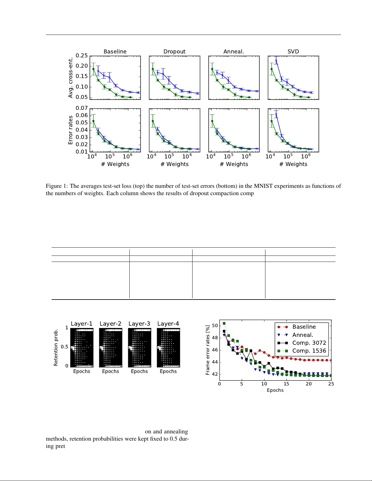
Compacting Neural Network Classifiers via Dr opout T raining Y otaro K ubo George T ucker Simon Wiesler Alexa Machine Learning, Amazon Abstract W e introduce dr opout compaction , a nov el method for training feed-forward neural netw orks which realizes the performance gains of training a large model with dropout re gularization, yet extracts a compact neural network for run-time efficienc y . In the proposed method, we introduce a sparsity-inducing prior on the per unit dropout retention probability so that the optimizer can ef- fectiv ely prune hidden units during training. By changing the prior hyperparameters, we can con- trol the size of the resulting network. W e per- formed a systematic comparison of dropout com- paction and competing methods on sev eral real- world speech recognition tasks and found that dropout compaction achiev ed comparable accu- racy with fewer than 50% of the hidden units, translating to a 2.5x speedup in run-time. Index T erms : Neural networks, dropout, model com- paction, speech recognition 1 Introduction Dropout [ 1 , 2 ] is a well-kno wn regularization method that has been used very successfully for feed-forward neural networks. Training lar ge models with strong regularization from dropout provides state-of-the-art performance on nu- merous tasks (e.g., [ 3 , 4 ]). The method inserts a “dropout” layer which stochastically zeroes indi vidual activ ations in the previous layer with probability 1 − p during training. At test time, these stochastic layers are deterministically approximated by rescaling the output of the pre vious layer by p to account for the stochastic dropout during training. Empirically , dropout is most effecti ve when applied to large models that would otherwise ov erfit [ 2 ]. Although training large models is usually not an issue anymore with multi- This manuscript was submitted to AIST A TS 2017. GPU training (e.g., [ 5 , 6 ]), model size must be restricted in many applications to ensure ef ficient test time ev aluation. In this paper , we propose a no vel form of dropout training that provides the performance benefits of dropout training on a large model while producing a compact model for de- ployment. Our method is inspired by annealed dropout train- ing [ 7 ], where the retention probability p is slowly annealed to 1 ov er multiple epochs. For our method, we introduce an independent retention probability parameter for each hidden unit with a bimodal prior distribution sharply peaked at 0 and 1 to encourage the posterior retention probability to con- ver ge to either 0 or 1 . Similarly to annealed dropout, some units will con verge to ne ver being dropped, howe ver , unlike annealed dropout, some units will conv erge to alw ays being dropped. These units can be remov ed from the network without accuracy de gradation. The annealing schedule and compaction rate of the resulting network can be controlled by changing the hyperparameters of the prior distribution. In general, model compaction has been well in vestigated. Con ventionally , this problem is addressed by sparsifying the weight matrices of the neural network. For example, [ 8 ] introduced a pruning criterion based on the second-order deriv ati ve of the objectiv e function. L1 regularization is also widely used to obtain sparse weight matrices. Howe ver , these methods only achiev e weight-lev el sparsity . Due to the relati ve ef ficiency of dense matrix multiplication com- pared to sparse matrix multiplication, these approaches do not improve test time efficienc y without degrading accu- racy . In contrast, our proposed method directly reduces the dimension of the weight matrices. In another approach, singular v alue decomposition (SVD) is used to obtain approximate low-rank representations of the weight matrices [ 9 ]. SVD can directly reduce the dimen- sionality of internal representations, howe ver , it is typically implemented as a linear bottleneck layer , which introduces additional parameters. This inef ficiency requires additional compression, which degrades performance. For example, if we are to compress the number of parameters by half, the SVD compacted model would hav e to restrict the internal dimensionality by 25%. Knowledge distillation can also be used to transfer kno wledge from larger models to a small model [ 10 ]. Howe ver , this requires two separate optimiza- tion steps that makes it difficult to directly apply to existing Manuscript was submitted to AIST A TS 2017 optimization configurations. [ 11 ] introduced additional mul- tiplicativ e parameters to the output of the hidden layers and regularize these parameters with an L1 penalty . This method is conceptually similar to dropout compaction in that both methods introduce regularization to reduce the dimension- ality of internal representations. Dropout compaction can be seen as an extension of this method by replacing L1 regularization with dropout-based re gularization. Similar to the SVD-based compaction technique, there are sev eral approaches for achieving faster ev aluation of neu- ral networks by assuming a certain structure in the weight matrices. For e xample, [ 12 ] introduces T oeplitz weight ma- trices as a building block of neural networks. [ 13 ] defines a structured matrix via discrete cosine transform (DCT) for enabling fast matrix multiplication via a fast F ourier trans- form algorithm. These methods successfully reduce the computational cost for neural network prediction; ho wev er , since those methods restrict the parameter space prior to training, these method may restrict the fle xibility of neural networks. Our proposed method attempts to jointly optimize the structure of the neural network and its parameters. This way , the optimization algorithm can determine an effecti ve low-dimensional representation of the hidden layers. Sev eral approaches for reducing numerical precision to speed up training and ev aluation hav e been proposed [ 14 , 15 , 16 ]. Most of these approaches are complemental with our method since our proposed method only changes the dimensionality of hidden layers, but the structure of the network stays the same. In particular, we also apply a ba- sic weight quantization technique in our experiments on automatic speech recognition tasks. The remainder of this paper is as follo ws: In Section 2, we introduce a probabilistic formulation of dropout training and cast it as an ensemble learning method. Then, we deriv e a method for optimizing the dropout retention probabilities p in Section 3. In Section 4, we present experimental results. In Section 5, we conclude the paper and suggest future extensions. 2 Con ventional Dr opout T raining In this section, we describe conv entional dropout training for feed-forward neural networks. Hereafter , we denote the input vectors by X = { x 1 , x 2 , · · · x T } , the target labels by K = { k 1 , k 2 , · · · k T } , and the parameters of a neural net- work by Θ def = { W ( ` ) ∈ R D ( ` ) × D ( ` − 1) , b ( ` ) ∈ R D ( ` ) | ` ∈ { 1 , .., L }} where L is the number of layers and D ( ` ) is the number of output units in the ` -th layer . 2.1 T raining Dropout training can be viewed as the optimization of a lower bound on the log-lik elihood of a probabilistic model. By introducing a set of random mask v ectors M def = { m ( ` ) ∈ { 0 , 1 } D ( ` ) | ` ∈ { 0 , .., L }} which defines a sub- set of hidden units to be zeroed, the output of a dropout neural network can be expressed as follo ws: h (0) ( x t ; M ) = m (0)  x t , h ( ` ) ( x t ; M ) = m ( ` )  a ( ` )  W ( ` ) h ( ` − 1) ( x t ; M ) + b ( ` )  , p ( k t | x t , M ) = exp  h ( L ) k t ( x t ; M )  P j exp  h ( L ) j ( x t ; M )  , (1) where  denotes element-wise multiplication, a ( ` ) is the ac- tiv ation function (usually a sigmoid or rectifier function) of the ` -th layer , and h ( L ) j denotes the j -th element in the vector function h ( L ) . The mask vectors are indepen- dent draws from a Bernoulli distribution (i.e., p ( M | Π ) = Q `,u ( π ( ` ) u ) m ( ` ) u (1 − π ( ` ) u ) 1 − m ( ` ) u ) parameterized by retention probability hyperparameters, Π def = { π ( ` ) ∈ [0 , 1] D ( ` ) | ` ∈ { 0 , .., L }} . In con ventional dropout training [ 1 , 2 ], all reten- tion probabilities belonging to the same layer are tied (i.e., π ( ` ) u = π ( ` ) u 0 for all possible ` , u and u 0 ). Optimizing the conditional log-likelihood of the target labels log p ( K |X , Θ , Π ) is intractable. Howe ver , a tractable lo wer bound can be used instead; log p ( K |X , Θ , Π ) = X t log p ( k t | x t , Θ , Π ) = X t log X M ∈M p ( k t | x t , M , Θ) p ( M | Π ) ≥ X t X M ∈M p ( M | Π ) log p ( k t | x t , M , Θ) , (2) where M is a set of all possible instances of M . A straight- forward application of stochastic gradient descent (SGD) applied to this lower bound leads to conv entional dropout training. 2.2 Prediction At test time, it is not tractable to mar ginalize over all mask vectors as in Eq. (2) . Instead, a crude (but fast) approxi- mation is applied. The av erage over all network outputs with all possible mask v ectors is replaced by the output of the network with the av erage mask, i.e. the vector m ( ` ) in Eq. (1) is replaced by the expectation v ector π ( ` ) : ˜ h (0) ( x t ; Π ) = π (0)  x t , ˜ h ( ` ) ( x t ; Π ) = π ( ` )  a ( ` )  W ( ` ) ˜ h ( ` − 1) ( x t ; Π ) + b ( ` )  . (3) Manuscript was submitted to AIST A TS 2017 In this way , we obtain an approximation of the predictive dis- tribution p ( k | x , Π , Θ) , which we denote by ˜ p ( k | x , Π , Θ) . In practice, this approximation does not degrade prediction accuracy [2]. 3 Retention Probability Optimization For le veraging the retention probabilities as a unit pruning criterion, we propose to untie the retention probability pa- rameters π ( ` ) u and put a bimodal prior on them. Then, we seek to optimize the joint log-likelihood log p ( K , Π |X , Θ) . In the next subsection, we compute the parameter gradients. In the second subsection, we describe the control variates we used to reduce variance in the gradients. Next, we de- scribe the prior we used to encourage the posterior retention probabilities to con ver ge to 0 or 1 . Finally , we summarize the algorithm. 3.1 Stochastic Gradient Estimation The joint log-likelihood is gi ven by log p ( K , Π |X , Θ) = log p ( K | Π , X , Θ) + log p ( Π ) = X t log X M ∈M p ( k t | x t , M , Θ) p ( M | Π ) + log p ( Π ) def = L (Θ; Π ) + log p ( Π ) , (4) where p ( Π ) is the prior probability distribution of the re- tention probability parameters. The objectiv e function with respect to the weight parameters Θ is unchanged (up to a constant), so we can follo w the con ventional dropout param- eter updates for Θ . The partial deriv ativ e of L with respect to the retention probability of the u -th unit in the ` -th layer is: ∂ L ∂ π ( ` ) u = X t X M ∈M p ( M | Π ) w t ( M )  ∂ ∂ π ( ` ) u log p ( M | Π )  = X t E p ( M | Π )  w t ( M )  ∂ ∂ π ( ` ) u log p ( M | Π )  , (5) where the weight function w is: w t ( M ) = p ( k t | x t , M , Θ) P M 0 ∈M p ( k t | x t , M 0 , Θ) p ( M 0 | Π ) . (6) Similarly to prediction in the conv entional dropout method, computing the denominator in the weight function is in- tractable due to the summation over all binary mask vectors. Therefore, we employ the same approximation, i.e. the de- nominator in Eq. (6) is computed using Eq. (3) . Hence, the weight function is approximated as: w t ( M ) ≈ p ( k t | x t , M , Θ) ˜ p ( k t | x t , Π , Θ) def = ˜ w t ( M ) . (7) The approximated weight function is computed by two feed forward passes: One with a stochastic binary mask and one with expectation scaling. The partial deriv ati ves of log p ( M | Π ) with respect to the retention probability parameters can be expressed as follows: ∂ ∂ π ( ` ) u log p ( M | Π ) = m ( ` ) u π ( ` ) u − 1 − m ( ` ) u 1 − π ( ` ) u . (8) 3.2 V ariance Reduction with Control V ariates The standard SGD approach uses an unbiased Monte Carlo estimate of the true gradient vector . Howe ver , the gradients of L (Θ; Π ) with respect to the retention probability param- eters exhibit high v ariance. W e can reduce the estimator’ s variance using control v ariates, closely following [ 17 , 18 ]. W e exploit the f act that E p ( M | Π )  ∂ ∂ π ( ` ) u log p ( M | Π )  = 0 , (9) cf. Eq. (8). This implies ∂ L ∂ π ( ` ) u = X t E p ( M | Π )  ( w t ( M ) − C ) ∂ ∂ π ( ` ) u log p ( M | Π )  (10) for any C that does not depend on M . Thus, an unbiased estimator is giv en by: ∂ L ∂ π ( ` ) u ≈ T |R| X r ∈R ( w t ( M r ) − C )  ∂ ∂ π ( ` ) u log p ( M r | Π )  , (11) where R is a random mini-batch of training data indices and M r is a set of mask vectors randomly drawn from p ( M | Π ) for each element in R . As before, we approximate w t ( M ) ≈ ˜ w t ( M ) to make the computation tractable. The optimal C does not hav e a closed-form solution. How- ev er , a reasonable choice for C is C = E p ( M | Π ) [ w t ( M )] = 1 (12) W ith this choice, we obtain an interpretable update rule: A training example ( x, k ) only contributes to an update of the retention probabilities Π if the predictiv e distribu- tion changes by applying a random dropout mask, i.e. if p ( k | x , M , Θ) 6 = ˜ p ( k | x , Π , Θ) . 3.3 Prior distribution of r etention probability In order to encourage the posterior to place mass on compact models, a prior distrib ution that strongly prefers π ( ` ) u = 1 or π ( ` ) u = 0 is required. W e use a powered beta distrib ution as the prior distribution p ( π ( ` ) u | α, β , γ ) ∝   π ( ` ) u  α − 1  1 − π ( ` ) u  β − 1  γ . Manuscript was submitted to AIST A TS 2017 Algorithm 1: Single update of retention probability Data: T raining data ( X , K ), neural net parameter Θ , initial values Π , random mini-batch R Data: Hyperparameters ( α , β , γ ), learning rate η , control variate C Result: Updated dropout probabilities Π // Derivative wrt log p ( Π ) for ` ∈ { 0 , .., L } , u ∈ { 1 , .., D ( ` ) } do δ ( ` ) u ← ∂ ∂ π ( ` ) u log p ( π ( ` ) u ) // Approx. derivative of log p ( k r | x r , Π ) for r ∈ R do M ← draw a mask from p ( M | Π ) ˜ w ← p ( k r | x r , M , Θ) ˜ p ( k r | x r , Π , Θ) // Eq. (7) δ ← δ + ( ˜ w − C ) ∇ Π [log p ( M | Π )] // Eq. (8) Π ← Clip [ Π + η δ ] // Clip computes max { 0 , min { 1 , x }} for each element x in the vector Computing the partition function is intractable when γ ( α − 1) ≤ 0 or γ ( β − 1) ≤ 0 . Ho wev er , computing the partition function is not necessary for SGD-based optimization. By setting α < 1 and β < 1 , the prior probability density goes to infinity as π ( ` ) u approaches 0 and 1 , respectively . Thus, we can encourage the optimization result to conv erge to either π ( ` ) u = 0 or π ( ` ) u = 1 . The exponent γ is intro- duced in order to control the relativ e importance of the prior distribution. By setting γ sufficiently large, we can ensure that the retention probabilities con ver ge to either 0 or 1 . 3.4 Algorithm Finally , the stochastic updates of the retention probabili- ties with control variates are summarized in Algorithm 1. In our experiments, we alternate optimization of the neu- ral network parameters Θ and the retention probabilities Π . Specifically , updates computed with Algorithm 1 are applied after each epoch of conv entional dropout training. Algo- rithm 2 shows the overall structure. After each epoch, we can remov e hidden units with retention probability smaller than a threshold without degrading performance. Therefore, we can already benefit from compaction during the training phase. 4 Experiments First, as a pilot study , we e valuated dropout compaction on the MNIST handwritten digit classification task. These experiments demonstrate the efficac y of our method on a widely used and publicly av ailable dataset. Next, we con- Algorithm 2: Alternating updates of DNN parameters Θ and retention probabilities Π Data: Training data ( X , K ), initial values Θ , Π Result: Updated dropout probabilities Π and neural net parameters Θ while performance impr oves do Optimize neural net parameters Θ (see [6] for detail) for R in the set of random batc hes in X do Π ← Algorithm1( X , K , Θ , Π , R ) Remov e hidden units with zero retention probability T able 1: Classification error rates and a verage test-set losses on the MNIST dataset for small and large netw orks. #W eights Err . rates [%] A vg. loss Small Baseline 42200 3 . 03 ± 0 . 167 0 . 156 ± 0 . 014 Dropout 42200 3 . 02 ± 0 . 181 0 . 164 ± 0 . 027 Annealing 42200 2 . 99 ± 0 . 119 0 . 157 ± 0 . 015 SVD 40400 3 . 25 ± 0 . 196 0 . 138 ± 0 . 011 82000 2 . 21 ± 0 . 161 0 . 123 ± 0 . 016 Compaction 46665.2 2 . 55 ± 0 . 188 0 . 101 ± 0 . 011 Large Baseline 477600 1 . 52 ± 0 . 089 0 . 0850 ± 0 . 004 Dropout 477600 1 . 50 ± 0 . 084 0 . 0818 ± 0 . 006 Annealing 477600 1 . 60 ± 0 . 091 0 . 0900 ± 0 . 005 SVD 357600 1 . 54 ± 0 . 083 0 . 0858 ± 0 . 004 795200 1 . 50 ± 0 . 030 0 . 0771 ± 0 . 004 Compaction 481276.7 1 . 49 ± 0 . 039 0 . 0536 ± 0 . 003 ducted a systematic ev aluation of dropout compaction on three real-world speech recognition tasks. In the experiments, we compared the proposed method against the dropout annealing method and SVD-based com- paction. Dropout annealing was chosen because the pro- posed method also varies the dropout retention probabilities while optimizing the DNN weights. The SVD-based com- paction method was chosen since this technique is widely used and applicable to many tasks. 4.1 MNIST The MNIST dataset consists of 60 000 training and 10 000 test images ( 28 × 28 gray-scale pixels) of handwritten digits. For simplicity , we focus on the permutation in variant version of the task without data augmentation. W e used 2 layer neural networks with rectified linear units (ReLUs). The parameters of the DNNs were initialized with random values from a uniform distribution with adaptiv e width computed with Glorot’ s formula [19] 1 . 1 W e also ev aluated with the ReL variant of Glorot’ s initializa- tion [ 20 ]; ho wev er , the ReL v ariant did not outperform the original Glorot initialization in our experiments. Manuscript was submitted to AIST A TS 2017 As is standard, we split the training data into 50 000 images for training and 10 000 images for hyperparameter optimiza- tion. Learning rates, momentum, and the prior parameters were selected based on de velopment set accurac y . The mini- batch size for stochastic gradient descent was set to 128 . W e ev aluated networks with v arious numbers of the hid- den units D ( ` ) ∈ { 25 , 50 , 100 , 200 , 400 , 800 , 1600 } . For dropout compaction training, we set β = α , to produce ap- proximately 50% compression. The SVD compacted mod- els were trained by applying SVD to the hidden-to-hidden weight matrices in the best performing neural networks in each configuration of D ( ` ) . The sizes of the bottleneck layer were set to d D ( ` ) / 8 e to achie ve 25% compression in terms of the number of the parameters in the hidden-to-hidden ma- trix. After the decomposition, the SVD-compacted networks were again fine-tuned to compensate for the approximation error . Based on manual tuning ov er the the development set accu- racies, the learning rate and momentum were set to 0 . 001 and 0 . 9 respectiv ely . L2 regularization was found not to be effecti ve for the baseline system. The optimal L2 reg- ularization constants were 10 − 6 for dropout and annealed dropout and 10 − 4 for dropout compaction. For the dropout annealing method, we increased the retention probability from 0 . 5 to 1 . 0 over the first 4 epochs. Figure 1 and T able 1 show the results of our proposed method and the other methods in comparison. In the figure, the plots in the first row sho w the differences in the av erage cross-entropy loss computed on the test set, and the plots in the second row sho w the dif ferences in the classification error rate. The green lines with “ o ” markers denote the pro- posed method and the blue lines with “ x ” markers denote the compared method, i.e. baseline feed forward net, con- ventional dropout, dropout annealing, and SVD compacted DNNs. The error bars in the plots represent two standard deviations ( ± 1 σ ) estimated from 10 trials with different random initialization. The table shows the results for small and large networks. The numbers of the weights in the table are the av erage numbers of the trials. In terms of test-set cross-entropy loss, dropout compaction performs consistently better than the other methods in com- parison. For the application to automatic speech recognition, which is our main interest, the performance in terms of cross- entropy loss is decisiv e, because the DNN is used as an estimator for the label probability (rather than a classifier). The behavior in terms of error rate differs. By increasing the model size, the error rate ev entually saturates at the same point for all methods. Howe ver , with small networks, dropout compaction also clearly outperforms the other meth- ods in terms of error rate. The case of small networks is the more relev ant one, because our aim is to apply dropout compaction for training small models. Here, "small" must be understood relativ e to the complexity of the task. Neural networks, which can be deployed in lar ge-scale production for dif ficult tasks like speech recognition, can typically be considered as small. 4.2 Large-V ocabulary Continuous Speech Recognition As an example of a real-world application, which requires large-scale deployment of neural networks, we applied dropout compaction to large-v ocabulary continuous speech recognition (L VCSR). W e performed experiments on three tasks: V oiceSearchLar ge, which contains 453h of voice queries, and V oiceSearchSmall, which is a 46h subset of V oiceSearchLar ge. GenericFarField contains 115h of far- field speech, where the signal is obtained by applying front- end processing to the seven channels from from a micro- phone array . W e used V oiceSearchSmall for conducting preliminary experiments for finding the optimal hyperpa- rameters, and used these for the other tasks. As input vectors to the DNNs, we extracted 32 dimensional log Mel-filterbank energies o ver 25ms frames e very 10ms. The DNN acoustic model processed 8 preceding, a middle frame, and 8 follo wing frames as a stacked vector (i.e., 32 × 17 = 544 dimensional input features for each target). Thus, with our feature extraction, the number of training examples is 16.5M (V oiceSearchSmall), 163M (V oiceSearchLarge), and 41M (GenericFarField), respecti vely . W e used a random 10% of the training data as a v alidation set, which was used for “Newbob”-performance based learn- ing rate control [ 21 ]. Specifically , we halved the learning rate when the improv ement from the last epoch is less than a threshold. As an analogy of cross validation-based model selection, we used 10% of the validation set for optimizing the retention probabilities. The baseline model size was designed such that the total ASR latency was belo w a certain threshold. The number of hidden units for each layer was determined to be 1 536 and the number of hidden layers was 4. The sigmoid activ ation function was used for nonlinearity in the hidden layers. Fol- lo wing the standard DNN/HMM-hybrid modeling approach, the output targets were clustered HMM-states obtained via triphone clustering. W e used 2 500, 2 506, and 2 464 clus- tered states with the V oiceSearchSmall, V oiceSearchLarge, and GenericFarField tasks, respecti vely . For fast e valuation, we quantized the values in the weight matrices and used integer operations for the feed-forw ard computations. These networks are suf ficiently small for achieving low latenc y in a speech recognition service. Therefore, in the experiments, we focus on two use cases: (a) Enabling the use of a larger network within the given fixed budget, and (b) achieving faster e valuation by compressing the current netw ork. All networks were trained with distributed parallel asyn- chronous SGD on 8 GPUs [ 6 ]. In addition, all net- Manuscript was submitted to AIST A TS 2017 0.05 0.10 0.15 0.20 0.25 Avg. cross-ent. Baseline 1 0 4 1 0 5 1 0 6 # Weights 0.01 0.02 0.03 0.04 0.05 0.06 0.07 Error rates Dropout 1 0 4 1 0 5 1 0 6 # Weights Anneal. 1 0 4 1 0 5 1 0 6 # Weights SVD 1 0 4 1 0 5 1 0 6 # Weights Figure 1: The averages test-set loss (top) the number of test-set errors (bottom) in the MNIST e xperiments as functions of the numbers of weights. Each column shows the results of dropout compaction compared to a con ventional feed-forward network, con v entional dropout, dropout annealing, and singular value decomposition, respectiv ely . The green lines with o marker and blue lines with x marker denote the results of proposed and the compared method, respecti vely . The error bars show ± 1 σ . T able 2: W ord error rates [%] on e valuation sets of the speech recognition tasks; the de velopment set error rates are shown in parentheses. Baseline Annealing SVD Compaction SVD Compaction # Hid. unit 1536 1536 (3072, 384) 3072 → ~1536 (1536, 192) 1536 → ~768 V oiceSearchSmall XEnt 22.5 (22.6) 22.3 (21.7) 22.5 (22.3) 21.8 ( 21.2 ) 22.7 (21.6) 22.6 (21.7) + bMMI 21.2 (21.0) 20.0 (19.8) 21.5 (21.1) 19.9 ( 19.7 ) 20.8 (20.3) 20.4 (19.8) V oiceSearchLarge XEnt 18.9 (18.2) 18.7 (18.2) 18.8 (18.2) 18.4 ( 18.0 ) 19.2 (18.8) 18.9 (18.5) + bMMI 17.9 (17.4) 17.2 ( 17.0 ) 17.7 (17.2) 16.9 ( 17.0 ) 17.3 (17.2) 17.3 (17.2) GenericFarField XEnt 24.0 (21.9) 23.6 (21.7) 24.4 (22.5) 23.4 ( 21.3 ) 24.8 (22.8) 23.9 (22.1) + bMMI 21.4 (19.7) 20.6 (18.8) 21.3 (19.1) 20.8 ( 18.7 ) 20.8 (18.9) 21.0 (18.9) Epochs 0 0.5 1 Retention prob. Layer-1 Epochs Layer-2 Epochs Layer-3 Epochs Layer-4 Figure 2: Evolution of histograms o ver retention probability in the first 12 epochs on V oiceSearchSmall. works were pretrained with the greedy layer-wise training method [ 22 ]. For the dropout compaction and annealing methods, retention probabilities were kept fix ed to 0.5 dur- ing pretraining. For annealed dropout, we use a schedule 0 5 10 15 20 25 Epochs 42 44 46 48 50 Frame error rates [%] Baseline Anneal. Comp. 3072 Comp. 1536 Figure 3: Frame error rates as a function of the number of epochs on V oiceSearchSmall. designed to increase the retention probabilities from 0.5 to Manuscript was submitted to AIST A TS 2017 1.0 in the first 18 epochs. As in the MNIST experiments, we fixed the hyperparameters to obtain approximately 50% compression 2 by setting α = β = 0 . 9 , and γ = T 0 where T 0 is the number of non-silence frames in the data set. Because con ventional dropout did not improve the perfor- mance of the baseline system in the ASR experiments, we only use annealed dropout as the reference system for dropout-based training. This may be due to the small size of the neural networks relati ve to our training corpus size. Fig. 2 sho ws histograms of the retention probabilities as functions of the numbers of epochs on the V oiceSearchS- mall task. As designed, the retention probabilities (initial- ized to 0.5) rapidly dif fused from the initial v alue 0 . 5 , and con ver ged to 0 or 1 in the first 11 epochs. W e did not ob- serve significant dif ferences with regard to the pruning rate and the con ver gence speed o ver dif ferent hidden layers. The compression rates of hidden layers were around 50% in all layers. Fig. 3 shows the ev olution of the frame error rate on the V oiceSearchSmall task. W e observed that annealed dropout started ov erfitting in the later epochs, after the retention probability was annealed to 1 . On the other hand, the dropout compaction methods exhibited the performance gain after the probabilities were con ver ged completely . This suggests that, similar to SVD-based compaction, our pro- posed method requires some fine-tuning after the structure is fixed, e ven though the fine-tune and compaction processes are smoothly connected in the proposed method. This might be the reason why the optimal prior parameters for dropout compaction, which were selected on the dev elopment set, implied that the retention probabilities con ver ge already in only 11 epochs, whereas the optimal parameters for dropout annealing yield a deterministic model after 18 epochs. T able 2 shows the word error rates ov er the dev elopment and ev aluation sets. As is standard in ASR, all cross- entropy models were fine-tuned according to a sequence- discriminativ e criterion, in this case the boosted maximum mutual information (bMMI) criterion [ 23 , 24 , 25 ]. Dropout compaction has been applied in the cross-entropy phase of the optimization, and the pruned structure was then used in the bMMI training phase. The results in T able 2 show that dropout compaction models starting with a larger structure (use case (a)) yielded the best error rates in all cases except for the bMMI result on the GenericFarField task and the y always performed better than the baseline. The differences were especially large in comparison to the cross-entropy trained models. The reason for this might be that the dropout compaction method determines the structure based on the cross-entropy-based 2 50% compression of hidden units yields roughly 25% com- pression of hidden-to-hidden weight matrices and 50% compres- sion of the input and output layer weight matrices. This leads to a roughly 2.5x speedup in the feed-forward computation. criterion. Regarding use case (b), dropout compaction achiev ed better results than the baseline network on all tasks. Further, most of the gains by annealed dropout are retained, although the dropout compaction models are roughly 2.5 times smaller . Compared to SVD-based model compaction, the proposed method performed better in almost all cases. Similar to the comparison in use case (a), the relativ e advantage of dropout compaction became smaller with the additional bMMI train- ing step. Therefore, adapting the proposed method to be compatible with sequence discriminativ e training such as bMMI is a promising future research direction. 5 Conclusion In this paper , we introduced dropout compaction, a novel method for training neural networks, which conv erge to a smaller network starting from a lar ger network. At At the same time, the method retains most of the performance gains of dropout regularization. The method is based on the estimation of unit-wise dropout probabilities with a sparsity-inducing prior . On real-world speech recognition tasks, we demonstrated that dropout compaction provides comparable accurac y ev en when the final network has fewer than 40% of the original parame- ters. Since computational costs scale proportionally to the number of parameters in the neural network, this results in a 2.5x speed up in ev aluation. In future work, we want to study whether the results by dropout compaction can be further improved by using more sophisticated methods for estimating the expectation over the mask patterns. Further , the application of our proposed method to con volutional and recurrent neural netw orks is a promising direction. References [1] G. E. Hinton, N. Sri vasta va, A. Krizhevsk y , I. Sutskev er , and R. R. Salakhutdinov , “Improving neural networks by prev enting co-adaptation of feature detectors, ” arXiv pr eprint arXiv:1207.0580 , 2012. [2] N. Srivasta va, G. Hinton, A. Krizhevsky , I. Sutske ver , and R. Salakhutdinov , “Dropout: A simple way to prevent neural networks from o verfitting, ” The Journal of Machine Learning Resear ch , vol. 15, no. 1, pp. 1929–1958, 2014. [3] A. Krizhevsky , I. Sutske ver , and G. E. Hinton, “Imagenet classification with deep con volutional neural networks, ” in Advances in Neural Infomr ation Pr ocessing Systems (NIPS) , 2012, pp. 1097–1105. [4] G. E. Dahl, T . N. Sainath, and G. E. Hinton, “Improving deep neural networks for L VCSR using rectified linear units and dropout, ” in Pr oc. of the IEEE Int. Conf. on Acoust., Speech, and Signal Pr ocess. (ICASSP) , V ancouver , Canada, May 2013, pp. 8609–8613. Manuscript was submitted to AIST A TS 2017 [5] F . Seide, H. Fu, J. Droppo, G. Li, and D. Y u, “1-bit stochas- tic gradient descent and its application to data-parallel dis- tributed training of speech DNNs, ” in Proc. of the Ann. Conf. of the Int. Speech Commun. Assoc. (Interspeech) , Sing apore, Sep. 2014, pp. 1058–1062. [6] N. Strom, “Scalable distributed dnn training using commod- ity GPU cloud computing, ” in Proc. of the Ann. Conf . of the Int. Speech Commun. Assoc. (Interspeech) , Dresden, Ger- many , Sep. 2015, pp. 1488–1492. [7] S. J. Rennie, V . Goel, and S. Thomas, “ Annealed dropout training of deep networks, ” in Proc. of the IEEE Spoken Language T echnology W orkshop (SLT) , 2014, pp. 159–164. [8] Y . LeCun, J. S. Denker , S. A. Solla, R. E. Howard, and L. D. Jackel, “Optimal brain damage, ” in Advances in Neur al Infomration Pr ocessing Systems (NIPS) , vol. 89, 1989, pp. 598–605. [9] J. Xue, J. Li, and Y . Gong, “Restructuring of deep neural network acoustic models with singular v alue decomposition, ” in Pr oc. of the Ann. Conf. of the Int. Speech Commun. Assoc. (Interspeech) , L yon, France, Aug. 2013, pp. 2365–2369. [10] G. Hinton, O. V inyals, and J. Dean, “Distilling the kno wledge in a neural network, ” arXiv pr eprint arXiv:1503.02531 , 2015. [11] K. Murray and D. Chiang, “ Auto-sizing neural networks: W ith applications to n -gram language models, ” in Pr oc. of the Confer ence on Empirical Methods in Natural Language Pr ocessing (EMNLP) , 2015, pp. 908–916. [12] V . Sindhwani, T . N. Sainath, and S. Kumar, “Structured transforms for small-footprint deep learning, ” in Pr oc. of the International Conference on Learning Representation (ICLR) , 2016. [13] M. Moczulski, M. Denil, J. Appleyard, and N. de Freitas, “A CDC: A structured efficient linear layer , ” in Pr oc. of the In- ternational Confer ence on Learning Representation (ICLR) , 2016. [14] S. Gupta, A. Agrawal, K. Gopalakrishnan, and P . Narayanan, “Deep learning with limited numerical precision, ” 2015. [15] M. Courbariaux, Y . Bengio, and J.-P . David, “Lo w precision arithmetic for deep learning, ” arXiv pr eprint arXiv:1412.7024 , 2014. [16] ——, “Binaryconnect: Training deep neural networks with binary weights during propagations, ” in Advances in Neural Infomration Pr ocessing Systems (NIPS) , 2015, pp. 3105– 3113. [17] J. Ba, R. R. Salakhutdinov , R. B. Grosse, and B. J. Frey , “Learning wake-sleep recurrent attention models, ” in Ad- vances in Neural Infomration Pr ocessing Systems (NIPS) , 2015, pp. 2575–2583. [18] A. Mnih and K. Gregor , “Neural variational inference and learning in belief networks, ” in Pr oc. of the International Confer ence on Machine Learning (ICML) , 2014, pp. 1791– 1799. [19] X. Glorot and Y . Bengio, “Understanding the difficulty of training deep feedforward neural networks, ” in Pr oc. of the International confer ence on artificial intelligence and statis- tics (AIST A TS) , 2010, pp. 249–256. [20] K. He, X. Zhang, S. Ren, and J. Sun, “Delving deep into rectifiers: Surpassing human-lev el performance on ImageNet classification, ” in Pr oc. of the International Confer ence on Computer V ision (ICCV) , 2015, pp. 1026–1034. [21] Quicknet. [Online]. A v ailable: http://www1.icsi.berkeley . edu/Speech/qn.html [22] Y . Bengio, P . Lamblin, D. Popovici, H. Larochelle et al. , “Greedy layer-wise training of deep networks, ” Advances in Neural Infomr ation Pr ocessing Systems (NIPS) , vol. 19, pp. 153–160, 2007. [23] D. Pov ey , D. Kanevsk y , B. Kingsbury , B. Ramabhadran, G. Saon, and K. V isweswariah, “Boosted MMI for model and feature-space discriminative training, ” in Proc. of the IEEE Int. Conf. on Acoust., Speech, and Signal Pr ocess. (ICASSP) , 2008, pp. 4057–4060. [24] B. Kingsbury , “Lattice-based optimization of sequence clas- sification criteria for neural-network acoustic modeling, ” in 2009 IEEE International Confer ence on Acoustics, Speech and Signal Pr ocessing . IEEE, 2009, pp. 3761–3764. [25] K. V esel ` y, A. Ghoshal, L. Burget, and D. Pov ey , “Sequence- discriminativ e training of deep neural networks. ” in Proc. of the Ann. Conf . of the Int. Speech Commun. Assoc. (Inter- speech) , 2013, pp. 2345–2349.