Tests for Comparing Weighted Histograms. Review and Improvements

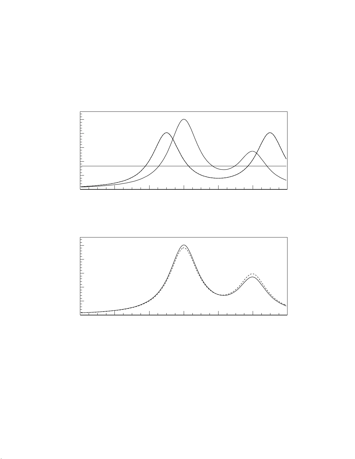
T ests for Comparing W eigh ted Histograms . Review and Impro v emen ts Nik olay D. Gagunash vili ∗ University of Ic eland, Sæmun dar gata 2, 101 R eykjavik, Ic eland Abstract Histograms w it h w eigh ted entries are used to estimate probability dens it y functions. Computer sim ulation is t he main application of this t yp e of his- tograms. A review on chi-sq uare tests for comparing we igh ted histogra ms is presen ted in this pap er. Impro ve men ts to t hese tests that ha ve a size closer to its nominal v alue are prop osed. Numerical examples are presen ted for ev aluation and demonstration of v arious applications of the tests. Key wor ds: homogeneit y test, random sum of random v ariables, fit w eigh ted histogram, Mon te-Carlo sim ulation. P A CS: 02.50.- r, 02.50.Cw, 02.50.Le, 0 2 .50.Ng 1. Intro duction A histogra m with m bins for a giv en probability densit y f unction (PDF ) p ( x ) is used to estimate the probabilities p i that a random ev en t b elongs to bin i : p i = Z S i p ( x ) dx, i = 1 , . . . , m. (1) In tegratio n in (1 ) is carr ied out ov er the bin S i and P m 1 p i = 1. A histogra m can b e obtained as a result of a random exp erimen t with the PDF p ( x ). A frequen tly used tec hnique in da t a analysis is to compare t w o distri- butions through comparison of histograms. The hypothesis of homogeneit y states that tw o histograms represen t random v alues with iden tical distribu- tions [1]. It is equiv alen t to the existing m c onstan ts p 1 , ..., p m , suc h that ∗ T el.: +35 45254 000; fax: + 35455 2133 1 Email addr ess: n ikola y@hi.i s (Nik olay D. Gagunashvili) Pr eprint submitt e d to Elsevier Septemb er 30, 2018 P m i =1 p i = 1, and the proba bility of b elonging to the i th bin for some mea- sured v alue in b o t h exp erimen t s is equal to p i . Let us denote the n umbers of random ev ents b elonging to the i th bin of the first and second histog r am as n 1 i and n 2 i , respectiv ely . The tota l n umber of ev en ts in the histograms is equal to n j = P m i =1 n j i , where j = 1 , 2. It has b een sho wn by Pearson [2] that the go o dness of fit test stat istic m X i =1 ( n j i − n j p i ) 2 n j p i (2) has approx imately a χ 2 m − 1 distribution. F or tw o statistically indep enden t histograms with probabilities p 1 , ..., p m , the statistic 2 X j =1 m X i =1 ( n j i − n j p i ) 2 n j p i (3) has a pproximately a χ 2 2 m − 2 distribution. If the probabilities p 1 , ..., p m are not kno wn, the estimation o f p i is carried out b y the follo wing expression: ˆ p i = n 1 i + n 2 i n 1 + n 2 , (4) as shown in [1]. By substituting expression (4) in (3), the statistic X 2 = 2 X j =1 m X i =1 ( n j i − n j ˆ p i ) 2 n j ˆ p i = 1 n 1 n 2 m X i =1 ( n 2 n 1 i − n 1 n 2 i ) 2 n 1 i + n 2 i (5) is obtained. This statistic has approximately a χ 2 m − 1 distribution b ecause m − 1 parameters are estimated [1]. The statistic (5) w a s first prop osed in [3] and is widely used to t est the h yp othesis of homogeneit y . A w eigh ted histogram or a histogram with w eigh ted eve n ts [4–6] is used to estimate the pr o babilities p i (1) as w ell. The sum of we igh ts o f ev en ts for the bin i is defined as: W i = n i X k =1 w i ( k ) , (6) where n i is the nu m b er of ev ents in the bin i a nd w i ( k ) is the w eigh t of the k th ev en t in the i th bin. The statistic ˆ p i = W i /n (7) 2 is used to estimate p i , where n = P m i =1 n i is a total num b er of eve nts for the histogram with m bins. W eigh ts of ev en ts are c hosen in suc h a w a y that the estimate (7) is un biased: E[ ˆ p i ] = p i . (8 ) Because of the condition P i p i = 1, w e will further call the ab ov e defined w eigh ts “normalized” as opp osed to the unnormalized w eights ˇ w i ( k ) whic h are ˇ w i ( k ) = const · w i ( k ). Comparison o f t wo w eigh t ed histogra ms and comparison of weigh ted and un w eigh ted histograms as w ell as fitting w eights of sim ulated random ev en ts to an exp erimen tal histogram are all imp ortan t parts of data analysis. T ests for comparing w eighte d histograms ha ve b een dev elop ed in [7, 8] while tests for Poiss o n w eighted histograms hav e b een prop osed in [9]. This pap er is or ganized as follows. In Section 2 generalization of the c hi-square homogeneit y test is discussed and improv emen ts for the test are prop osed. A test for his t ograms with unnor ma lized w eigh ts as w ell as im- pro vem en ts of that test are discussed in Section 3. T ests for comparison of t wo P oisson w eighted histograms are discussed in Section 4. R estrictions f o r c hi-square test application are discussed in Section 5. Applications and v er- ification of the t ests are demonstrated using n umerical examples in Section 6. 2. Homogeneity test for comparison tw o histograms with normal- ized weigh t s Let us consider t w o histograms with normalized w eigh ts, and the subinde x j will b e used to differen t iate them. A to tal sum of w eights of ev en ts W j i in the i th bin of the j th histogram j = 1 , 2; i = 1 , . . . , m can b e considered as a sum of random v aria bles W j i = n j i X k =1 w j i ( k ) , (9) where the n um b er of ev ents n j i is also a random v alue a nd the w eights w j i ( k ) , k = 1 , ..., n j i are indep enden t random v a r ia bles with the same PDF for a giv en bin [4, 6 ]. Let us intro duce a v ariable r j i = E [ w j i ] / E[ w 2 j i ] , (10) 3 whic h is the ratio of t he first momen t to the second momen t of the distribu- tion of w eights in the bin i . Let us estimate r j i using ˆ r j i = n j i X k =1 w j i ( k ) / n j i X k =1 w 2 j i ( k ) . (11) As show n in [4] the statistic 1 n j X i 6 = k ˆ r j i W 2 j i p i + 1 n j ( n j − P i 6 = k ˆ r j i W j i ) 2 1 − P i 6 = k ˆ r j i p i − n j , (12) where sums extend o ver all t he bins i , except fo r the bin k , whic h has appro x- imately a χ 2 m − 1 distribution and is a generalization of the P earson’s statistic (2) [4, 6, 10]. It should b e noted that it is only v alid for the case when 1 − P i 6 = k ˆ r j i p i > 0. The la st inequality means that estimation of a co v ar ia nce matrix fo r v ariables W j 1 , ..., W j k − 1 , W j k +1 , ..., W j m is p ositiv e definite. The b etter p ow er of test, as w as shown in [6 ], w a s ac hiev ed f or k j , where k j = argmin i ˆ p i ˆ r j i . (13) 2.1. Me dia n test statistic for c omp arison of wei ghte d histo gr ams with nor- malize d weights F ollo wing [7], for tw o statistically indep enden t histograms with pro babil- ities p 1 , ..., p m the statistic has approx imately a χ 2 m − 1 distribution: ˆ X 2 k = 2 X j =1 1 n j X i 6 = k ˆ r j i W 2 j i ˆ p i + 2 X j =1 1 n j ( n j − P i 6 = k ˆ r j i W j i ) 2 1 − P i 6 = k ˆ r j i ˆ p i − 2 X j =1 n j . (14) The probabilities p i are not know n and estimators ˆ p 1 , . . . , ˆ p k − 1 , ˆ p k +1 , . . . , ˆ p m can b e determined by minimizing (14 ) under the follo wing constraints : ˆ p i > 0 , 1 − X i 6 = k ˆ p i > 0 , 1 − X i 6 = k ˆ r 1 i ˆ p i > 0 , and 1 − X i 6 = k ˆ r 2 i ˆ p i > 0 . (15) The problem to determine the estimators of the probabilities ˆ p i b y mini- mizing (14) has b een solved n umerically by co ordinate-wise optimization in [7, 8]. F or ev ery step, the minim um for one probability with others fixed ones can b e found using t he Bren t algorithm [11]. 4 A test statistic obtained as a median v alue of the form ula (14) for a differen t choice of the excluded bin ˆ X 2 M ed = Med { ˆ X 2 1 , ˆ X 2 2 , . . . , ˆ X 2 m } (16) w as prop o sed in [7, 8 ] and has approximately a χ 2 m − 1 distribution if the h yp othesis of homogeneity is v alid. The median is calculated for the set of s tatistically dep enden t random v aria bles ˆ X 2 i , with eac h v ariable having approximately χ 2 m − 1 distribution [6, 10]. The median statistic (16) coincides with the statistic (5) in case of tw o histograms with un weigh ted en tries. Numerical in ves tigations of the median tests (see Section 6.1 and Ref. [4]) sho w that the size of the test (16) exceeds sligh t ly its nominal v alue mak ing it the main disadv antage of this approac h. The question, what deviation from the no minal size is acceptable for chi-sq uare metho ds, has differen t answ ers. In the classical w ork dedicated to c hi- square tests [17] disturbance is re- garded as unimp ortant when the nominal size of a test is 5%, with the exact size lying b etw een 4% and 6%, a nd when the nominal size o f a test is 1%, with the exact size lying b etw een 0 . 7% a nd 1 . 5 %. According t o this criteria the disturbance of the median test can b e considered unimp orta nt. Ho we v er, according to [9], the disturbance of the median statistics is im- p ortant. The a ut ho rs of [9] ha ve prop o sed tests for comparison of histogr a ms of an e quiva lent numb er of unweighte d events with false in t erpretation of these tests as tests for histograms with weigh ted en tries. The metho ds from [9] are discusse d in section 4 with n umeric ev aluation sho wn in subsection 6.2.1. 2.2. New test statistic for c omp arison of weighte d histo gr ams with normali ze d weights The median test (16) can b e improv ed by using the results for go o dness of fit test for w eigh ted histogra ms [6]. The new test statistic is ˆ X 2 = 2 X j =1 1 n j X i 6 = k j ˆ r j i W 2 j i ˆ p i + 2 X j =1 1 n j ( n j − P i 6 = k j ˆ r j i W j i ) 2 1 − P i 6 = k j ˆ r j i ˆ p i − 2 X j =1 n j . (17) The estimation of the probabilities ˆ p 1 , . . . , ˆ p m is determined by minimizing (17) under the follo wing constraints : ˆ p i > 0 , X i ˆ p i = 1 , 1 − X i 6 = k 1 ˆ r 1 i ˆ p i > 0 , and 1 − X i 6 = k 2 ˆ r 2 i ˆ p i > 0 , (18) 5 where k j is defined as k j = argmin i ˆ p i ˆ r j i . (19) The test statistic asymptotically has a χ 2 m − 1 distribution a nd a size closer to its nominal v alue than the test (16) if the h yp ot hesis of homogeneity is v alid. The bin k j with the lo w est information con ten t is excluded to get the robust stat istic ˆ X 2 and it is plausible that the tes t (17) has higher pow er than the median test ( 1 6). Detail explanation o f this c ho ice is presen ted in Subsection 2 .3 of [6 ]. 3. Homogeneity test for histogr ams wit h unnormalized weigh t s In pra ctice one is often confron ted with cases when a histogram is defined up to a n unknown normalization constan t. Let us denote bin conte n t of histograms with unnormalized w eights as ˇ W j i , t hen W j i = ˇ W j i C j , a nd the test statistic (12) can b e written as C j n j X i 6 = k ˇ r ij ˇ W 2 j i p i + 1 n j ( n j − P i 6 = k ˇ r j i ˇ W j i ) 2 1 − C − 1 j P i 6 = k ˇ r j i p i − n j , (20) with ˇ r j i = C j r j i . An estimator ˆ C j k for the constan t C j is found in [4] b y minimizing (20) and is equal to ˆ C j k = X i 6 = k ˇ r j i p i + s P i 6 = k ˇ r j i p i P i 6 = k ˇ r j i ˇ W 2 j i /p i ( n j − X i 6 = k ˇ r j i ˇ W j i ) . (21) Substituting (21) for (20) and replacing ˇ r j i with the estimate ˆ ˇ r j i w e get the test statistic ˆ C j k n j X i 6 = k ˆ ˇ r j i ˇ W 2 j i p i + 1 n j ( n j − P i 6 = k ˆ ˇ r j i ˇ W j i ) 2 1 − C − 1 j P i 6 = k ˆ ˇ r j i p i − n j , (22) The estimate ˆ ˇ r j i in (22) is calculated in the same wa y as the estimate ˆ r j i in (11). The stat istic (22) has approximately a χ 2 m − 2 distribution. 6 3.1. Me dia n test statistic for c omp arison of weighte d histo gr ams with unnor- malize d weights F ollo wing [7], for tw o statistically indep enden t histograms with pro babil- ities p 1 , ..., p m , the statistic ˆ ˇ X 2 k = 2 X j =1 ˆ C j k n j X i 6 = k ˆ ˇ r j i ˇ W 2 j i ˆ p i + 1 n j ( n j − P i 6 = k ˆ ˇ r j i ˇ W j i ) 2 1 − ˆ C − 1 j k P i 6 = k ˆ ˇ r j i ˆ p i − n j , (23) has approx imately a χ 2 m − 2 distribution. An estimation of the pro babilities ˆ p 1 , . . . , ˆ p k − 1 , ˆ p k +1 , . . . , ˆ p m can b e found b y minimizing (23) under the follo wing constrain ts: ˆ p i > 0 , 1 − X i 6 = k ˆ p i > 0 , 1 − ˆ C − 1 1 k X i 6 = k ˆ r 1 i ˆ p i > 0 , and 1 − ˆ C − 1 2 k X i 6 = k ˆ r 2 i ˆ p i > 0 . (24) The probabilities ˆ p i can b e c alculated n umerically in the s ame w a y as de- scrib ed in Section 2. A test statistic that is “in v ariant” to the c hoice of the excluded bin can b e obtained again as a median v alue of (25) for a ll p ossible c hoices of t he excluded bin ˆ ˇ X 2 M ed = Med { ˆ ˇ X 2 1 , ˆ ˇ X 2 2 , . . . , ˆ ˇ X 2 m } . (25) The statistic 1 ˆ ˇ X 2 M ed for the case of comparing t wo histograms with normalized and unnormalized w eights can b e giv en b y the same form ulas (2 3 – 25 ) with C 1 k ≡ 1. Both statistics ˆ ˇ X 2 M ed and 1 ˆ ˇ X 2 M ed ha ve a ppro ximately a χ 2 m − 2 distribution if the h yp o t hesis of homogeneity is v alid. 3.2. New test statistic for c omp aris on of weighte d histo gr ams with unnormal- ize d weights The median test (25) can b e improv ed by using the results for go o dness of fit test for w eigh ted histogra ms [6]. A new test statistic is ˆ ˇ X 2 = 2 X j =1 ˆ C j k j n j X i 6 = k j ˆ ˇ r j i ˇ W 2 j i ˆ p i + 1 n j ( n j − P i 6 = k j ˆ ˇ r j i ˇ W j i ) 2 1 − ˆ C − 1 j k j P i 6 = k j ˆ ˇ r j i ˆ p i − n j . (26) 7 Estimation of the probabilities ˆ p i can b e determined b y minimizing (26) under the follow ing constrain ts: ˆ p i > 0 , X i ˆ p i = 1 , 1 − ˆ C − 1 1 k 1 X i 6 = k 1 ˆ r 1 i ˆ p i > 0 , and 1 − ˆ C − 1 2 k 2 X i 6 = k 2 ˆ r 2 i ˆ p i > 0 , (27) where k j is defined as k j = argmin i ˆ p i ˆ r j i . (28) The test statistic asymptotically has a χ 2 m − 2 distribution a nd a size closer to its nominal v alue. It is plausible that the test (26) has higher p o wer than the test (25). The statistic 1 ˆ ˇ X 2 for the case of compar ing t w o histograms with normal- ized a nd unnormalized we ig h ts c an b e giv en by the same form ulas (2 6 – 28 ) with C 1 k 1 ≡ 1. Both statistics ˆ ˇ X 2 and 1 ˆ ˇ X 2 ha ve appro ximately a χ 2 m − 2 distribution if the h yp othesis of homogeneity is v alid. 4. T est for comparison of weigh ted P oisson histograms A Poisson histogram [12, 13] is defined as a histogram with m ulti-Poiss o n distributions of a n umber of ev en ts for bins: P ( n 1 , . . . , n m ) = m Y i =1 e − n 0 p i ( n 0 p i ) n i /n i ! , (29) where n 0 is a free para meter. The probability distribution function (29) can be represen ted as a pro duct of tw o probability functions: a P oisson probabilit y distribution function f or a num b er of ev en ts n with the parameter n 0 and a multinomial pro babilit y distribution function of a num b er of ev ents for bins of the histogram, with a total num b er of ev en ts equal to n [12 , 13]: P ( n 1 , . . . , n m ) = e − n 0 ( n 0 ) n /n ! × n ! n 1 ! n 2 ! . . . n m ! p n 1 1 . . . p n m m . (30) A P oisson histogram can b e obta ined as a result of t wo random exp eri- men ts, namely when a first experiment with a Pois son probability distribu- tion function gives us a total n umber of ev en ts in the histogram n and then 8 a histogram is obta ined as a r esult of a random exp erimen t with a PDF p ( x ) and with a total num b er of eve n ts equal to n . The concept o f a n e quivalent numb er of unw eighte d events has b een in- tro duced in [9]. An e quivale nt numb er of unweighte d events for i th bin of w eigh ted histogram is W i r i . The authors prop o sed t w o test statistics for com- parison of histograms with e quivalent numb er of unweighte d events conten ts of bins. These statistics were in terpreted in [9] as statistics for comparison of orig ina l P o isson w eigh t ed histograms. 4.1. First statistic for c omp aring Poisson weighte d histo gr ams The first statistic X 2 p 1 , in our notation, can b e written as X 2 p 1 = C − 1 m X i =1 ( W 1 i − C W 2 i ) 2 W 1 i r − 1 2 i + W 2 i r − 1 1 i . (31) The parameter C [9] is ta k en equal to C = P W 1 i P W 2 i . (32) The stat istic (3 1) according to [9] has a χ 2 m distribution if the hypothesis of homogeneit y is v a lid. 4.2. Se c on d statistic for c omp aring Poisson we ighte d histo gr ams The parameter C can also b e estimated [9]. Here an es timator ˆ C w as found by minimizing (31) a nd is equal t o ˆ C = s X W 2 1 i W 1 i r − 1 2 i + W 2 i r − 1 1 i  X W 2 2 i W 1 i r − 1 2 i + W 2 i r − 1 1 i  − 1 . (33) The second statistic X 2 p 2 = ˆ C − 1 m X i =1 ( W 1 i − ˆ C W 2 i ) 2 W 1 i r − 1 2 i + W 2 i r − 1 1 i (34) has a χ 2 m − 1 distribution if the h yp othesis of ho mo g eneit y is v alid [9]. 9 5. Restr ictions of chi- square t est applications The use of the c hi-square test X 2 (5) for the histograms with un w eigh ted en tries is inappropriate if any exp ected frequency n 1 ˆ p i or n 2 ˆ p i < 1 or if the total n umber of bins with the exp ected fr equency n 1 ˆ p i or n 2 ˆ p i < 5 exceeds 20% of the to tal num b er (2 m ) of bins [16, 17]. Restrictions for w eigh ted histograms can b e obtained by replacing the ab ov e men tioned exp ected frequencies with expected fr equencies o f the e quiv- alent numb er of unwe ighte d events . F or the test ˆ X 2 (17) they m ust b e replaced with n 1 ˆ p i ˆ r 1 i and n 2 ˆ p i ˆ r 2 i , while for the test ˆ ˇ X 2 (26) with n 1 ˆ p i ˆ r 1 i /C 1 k 1 and n 2 ˆ p i ˆ r 2 i /C 2 k 2 . 6. Ev aluation of the tests’ sizes and p o wer The h yp othesis of homogeneity H 0 is rejected if the v alue of the test statistic ˆ X 2 is ab o v e a giv en threshold. The threshold k α for a give n nominal size of the test α can b e defined fro m the equation α = P ( χ 2 l > k α ) = Z + ∞ k α x l/ 2 − 1 e − x/ 2 2 l/ 2 Γ( l / 2) dx, (35) where l = m − 1. Let us define t he test size α s for a g iv en nominal size of the test α as the probabilit y α s = P ( ˆ X 2 > k α | H 0 ) , (36) i.e. the proba bility that the hy p othesis H 0 will b e rejected if the distribution of the w eigh ts W j i , j = 1 , 2 ; i = 1 , ..., m , for the bins of the histogra ms satisfies the h yp othesis H 0 . The deviation of a test size from its nominal v alue is an imp orta n t test c haracteristic. A second imp ort a n t c haracteristic of the test is its p o w er β β = P ( ˆ X 2 > k α | H a ) , (37) i.e. the probabilit y that the h yp othesis of homogeneit y H 0 will b e r ejected if the distributions of the we igh ts W j i , j = 1 , 2; i = 1 , ..., m o f the compared histograms do not satisfy the hypothesis H 0 . The same definitions with l = m − 2 in the form ula (35) can b e used for the test statistic ˆ ˇ X 2 (26). 10 Let us consider an example of a w eighted histogram for estimation of the probabilit y p i (1) for a giv en PDF p ( x ) in the form p i = Z S i p ( x ) dx = Z S i w ( x ) g ( x ) dx, (38) where w ( x ) = p ( x ) /g ( x ) (39) is a weigh t function and g ( x ) is some o ther PDF. The function g ( x ) m ust b e > 0 for the p oin ts x , where p ( x ) 6 = 0. The w eigh t is equal to 0 if p ( x ) = 0 [14]. A w eighted histogra m is a histogram obtained from a random exp erimen t with the PDF g ( x ), and the w eigh ts of the ev en ts are calculated according to (39). T o ev aluate a size and p o wer of the tests let us tak e the distribution p ( x ) ∝ 2 ( x − 1 0) 2 + 1 + 1 ( x − 1 4) 2 + 1 (40) defined on the in terv al { 4 , 16 } and repres en ted b y t w o Breit-Wigner p eaks [15]. Three cases of the PD F g ( x ) can b e considered (Fig. 1): g 1 ( x ) = p ( x ) (41) g 2 ( x ) = 1 / 1 2 (42) g 3 ( x ) ∝ 2 ( x − 9 ) 2 + 1 + 2 ( x − 1 5) 2 + 1 (43) The distribution g 1 ( x ) (41) results in a histogram with un w eighted en t r ies, while the distribution g 2 ( x ) (42) is a uniform distribution on the in terv a l { 4 , 16 } . The distribution g 3 ( x ) (43) has the same f orm of parametrization as p ( x ) (4 0), but with differen t v a lues of the pa rameters. Sizes o f the tests for histograms with a num b er of bins eq ua l t o 5 and differen t w eighted functions w ere calculated for the nominal size α equal to 0.05. Calculations o f the test sizes α s w ere carried out using the Mon te Carlo metho d with 10 000 runs, therefore it is reasonable to test the h yp o thesis 11 H (1) 0 : α s = 0 . 05 against the alternat ive H (1) a : α s 6 = 0 . 05 . F or this purp ose z statistics can b e used [1 6 ] z = ( ˆ α s − 0 . 05) / r 0 . 05 × (1 − 0 . 05) 10 000 , (44) where ˆ α s is an estimated v alue of α s . If the n ull h yp othesis is true then this test statistic has a standard normal distribution. F or the standar d no rmal distribution, 2.5% of the v alues lie b elow the critical v alue of − 1 . 9599 6 4, and 2.5% lie a b ov e 1.959 964. There fore, if a 2- sided hy p othesis test is conducted with a significance lev el equal to 0.05 , H (1) 0 is accepted when | z | ≤ 1 . 9599 64 or 0 . 04 5 728 ≤ ˆ α s ≤ 0 . 0 54272. The results of calculation for a pair of histograms with either no rmalized w eigh ts or unnormalized we igh ts a s w ell as for tw o histogra m with normal- ized and unnor ma lized we igh ts are pr esen ted in T ables 1 – 6 fo r different we ig h t functions, and differen t total n um b er of ev ents. T o calculate sizes o f tests t wo statistically indep enden t w eigh ted histograms we re sim ulated. The dis- tribution p ( x ) (4 0) was used for sim ulation of the first w eigh ted his togram and the same distribution p ( x ) for sim ulation o f the second one. W eigh ts p ( x ) /g i ( x ) where used for histograms with normalized w eighted en tries as w ell as w eigh ts 2 p ( x ) /g i ( x ) and 3 p ( x ) /g j ( x ) for histograms with unnormalized w eigh ted en tries. P ow ers of the tests were in v estigated for slightly differen t v alues of the amplitude of the second p eak of the sp ecified probability distribution function (Fig. 2): p 0 ( x ) ∝ 2 ( x − 10) 2 + 1 + 1 . 15 ( x − 14) 2 + 1 . (45) 6.1. T ests for histo gr ams with a m ultinomial distribution of events A size o f the tests w as calculated for a differen t tota l n umber o f ev en ts n 1 and n 2 in fiv e bin histograms. In the following, n umerical examples demon- strate a pplicatio ns of: • The median test X 2 M ed (16) and the new test ˆ X 2 (17) fo r compar ison of w eigh ted histograms with normalized w eigh ts (T a ble 1); • The median test ˆ ˇ X 2 M ed (25) and the new test ˆ ˇ X 2 (26) for comparison of w eigh ted histograms with unnormalized weigh ts (T able 2); 12 • The median test 1 ˆ ˇ X 2 M ed (25) and the new test 1 ˆ ˇ X 2 (26) fo r comparison of a w eigh ted histog ram with no rmalized w eigh ts and a histogram with unnormalized w eigh ts (T able 3). 0 0.05 0.1 0.15 0.2 0.25 4 6 8 10 12 14 16 g 1 (x) g 3 (x) g 2 (x) x Figure 1: P robability densit y functions g 1 ( x ) = p ( x ), g 2 ( x ) = 1 / 12 and g 3 ( x ). 0 0.05 0.1 0.15 0.2 0.25 4 6 8 10 12 14 16 p(x) p 0 (x) x Figure 2: P robability densit y functions p ( x ) (solid line) a nd p 0 ( x ) (dashed line). 13 T able 1: Sizes ˆ α s of the test ˆ X 2 M ed (16) for c o mparison of t wo histo grams with normalized weigh ted e n tries (left panel) and sizes of the new test ˆ X 2 (17) (rig ht panel) for different pairs of weights (las t column) a nd num b er s of even ts n 1 , n 2 . Size s o f the tests that do not sa tis fy the hypo thesis α s = 5 % with a significa nce level equal to 0 . 0 5 ( ˆ α s > 5 . 4 % or ˆ α s < 4 . 6%) are hig hlighted with gr ay . n 2 n 2 n 1 200 400 800 1600 3200 6400 200 400 800 1600 3200 6400 w ( x ) 200 4.9 4.5 4.7 4.6 5.2 4.9 4.2 4.7 4.6 4.9 4.6 4.8 400 4.7 4.7 4.8 4.7 5.1 5.0 4.4 4.7 4.4 4.8 5.2 5.2 1 800 4.9 4.5 4.7 4.9 5.3 4.4 4.8 4.7 4.5 5.0 5.3 4.9 & 1600 5.2 4.7 5.3 4.7 5.5 5.1 4.4 4.9 5.0 4.9 4.9 5.0 3200 4.9 5.0 5.0 4.7 4.8 4.9 5.2 5.3 5.0 4.9 4.9 4.8 1 6400 5.2 5.3 5.0 5.0 5.2 5.3 5.2 5.1 4.8 5.5 4.8 5.0 200 5.5 5.7 5.1 5.0 5.1 5.1 4.7 4.9 5.2 5.0 5.0 4.6 1 400 5.5 5.7 5.4 5.8 5.2 5.2 5.2 5.4 5.0 5.1 4.8 5.0 800 5.7 5.8 5.5 5.8 4.8 5.0 5.1 5.1 5.1 5.1 5.2 5.2 & 1600 5.3 5.5 5.7 5.2 4.9 4.9 5.4 5.5 5.4 5.1 5.2 5.2 p ( x ) g 2 ( x ) 3200 5.4 5.3 5.4 5.6 5.3 5.4 5.6 5.5 5.1 4.9 4.8 4.8 6400 5.6 5.5 5.4 5.3 5.3 5.3 5.5 4.8 5.1 5.1 5.1 5.0 200 5.0 4.8 5.0 4.9 4.8 5.3 5.3 5.0 4.7 4.7 4.7 4.7 1 400 5.3 5.1 5.0 5.2 5.4 5.1 5.7 5.6 5.4 5.1 4.9 4.9 800 5.4 5.6 5.2 5.5 5.2 5.0 5.5 4.8 5.0 5.0 4.9 4.5 & 1600 5.7 5.4 5.5 5.3 5.6 5.5 5.7 5.5 5.1 5.0 5.3 5.2 p ( x ) g 3 ( x ) 3200 5.9 5.3 5.6 5.5 5.3 5.3 6.2 5.5 5.4 5.1 5.1 5.1 6400 6.1 5.6 5.4 5.4 5.5 5.3 5.6 6.2 5.1 5.0 5.0 5.2 200 5.5 5.2 5.5 6.1 5.9 5.8 5.7 5.3 5.5 5.2 5.5 5.0 p ( x ) g 2 ( x ) 400 5.3 5.3 5.8 5.5 5.7 5.3 5.8 5.1 5.0 5.1 4.7 5.0 800 6.0 6.1 5.5 5.3 5.2 5.8 5.9 5.4 5.0 5.2 5.2 5.4 & 1600 5.7 5.5 5.7 5.1 5.2 5.2 5.3 5.6 5.2 4.8 5.2 4.7 p ( x ) g 2 ( x ) 3200 5.7 5.3 5.1 5.5 5.1 5.6 5.5 5.3 4.7 5.1 4.6 4.4 6400 5.5 5.6 5.8 5.6 5.3 5.0 5.4 5.2 5.0 4.9 5.1 5.2 200 5.7 5.8 6.1 5.7 5.6 5.6 5.7 5.7 5.6 5.4 5.1 5.4 p ( x ) g 2 ( x ) 400 5.5 5.0 5.1 5.6 5.2 5.8 5.2 5.6 5.5 5.1 5.2 4.7 800 5.4 5.6 5.2 5.6 5.5 5.5 5.9 5.0 5.2 4.9 5.1 4.8 & 1600 5.3 5.6 5.7 5.5 5.6 5.7 5.5 5.3 5.0 5.3 5.2 5.4 p ( x ) g 3 ( x ) 3200 6.1 5.9 5.1 5.5 5.4 5.6 5.5 5.4 5.4 4.8 4.9 4.9 6400 5.9 5.4 5.6 5.8 5.5 5.5 6.5 5.5 5.3 5.5 5.1 5.3 200 5.0 5.2 5.8 5.7 5.9 6.0 5.5 6.0 5.8 6.0 5.8 6.1 p ( x ) g 3 ( x ) 400 5.3 5.5 5.6 5.5 5.8 5.6 5.6 5.1 5.0 5.3 5.5 5.5 800 5.6 5.4 5.4 5.5 5.6 5.8 5.8 5.0 5.1 5.0 5.1 5.3 & 1600 6.2 5.2 5.8 5.3 5.4 5.6 5.4 5.6 5.2 4.9 4.9 5.0 p ( x ) g 3 ( x ) 3200 6.1 5.9 5.3 5.9 4.9 5.2 5.9 5.6 5.2 5.1 4.8 5.4 6400 6.1 5.5 6.0 5.5 4.7 5.5 5.9 5.5 5.3 4.9 5.1 4.9 T able 2: Sizes ˆ α s of the test ˆ ˇ X 2 M ed (25) for compar ison o f tw o histogra ms with unnor- malized weight ed ent ries (left panel) a nd sizes o f the new test ˆ ˇ X 2 (26) (right panel) for different pair s of weigh ts (last column) and n umbers of e vents n 1 , n 2 . Sizes of the tests that do not satisfy the hypothesis α s = 5% with a significance level equal to 0 . 05 ( ˆ α s > 5 . 4% or ˆ α s < 4 . 6%) are hig hlighted with gr ay . n 2 n 2 n 1 200 400 800 1600 3200 6400 200 400 800 1600 3200 6400 w ( x ) 200 5.8 5.6 5.5 6.2 6.3 5.8 4.9 5.1 5.0 5.0 5.2 5.6 2 p ( x ) g 2 ( x ) 400 5.6 5.7 6.0 5.8 5.7 5.6 4.7 4.8 5.4 5.2 4.9 4.9 800 6.0 6.1 5.8 6.0 5.5 6.1 5.2 5.2 5.0 5.1 5.1 4.8 & 1600 5.9 5.6 6.0 5.5 5.7 5.7 4.8 4.9 5.0 4.9 5.2 5.1 3 p ( x ) g 2 ( x ) 3200 5.9 5.5 5.5 5.9 5.6 6.0 5.5 5.3 4.6 4.9 5.0 5.0 6400 5.8 5.7 5.8 6.1 5.7 5.4 5.2 5.2 5.0 4.8 5.1 5.1 200 5.2 5.7 5.9 5.7 5.7 5.9 5.0 5.1 4.6 5.0 4.9 5.4 2 p ( x ) g 2 ( x ) 400 5.5 5.1 5.3 5.9 5.6 5.9 5.1 5.7 5.2 5.3 5.1 4.9 800 5.2 5.8 5.6 5.8 5.8 5.6 5.2 5.2 4.6 4.9 4.7 5.0 & 1600 5.3 5.5 5.8 5.7 5.8 5.9 5.3 4.9 5.0 5.4 4.4 4.7 3 p ( x ) g 3 ( x ) 3200 5.5 5.8 5.2 5.4 5.6 6.1 4.6 5.3 5.1 5.1 4.6 5.2 6400 5.5 5.2 5.6 6.1 5.6 5.8 4.8 5.1 4.7 4.9 4.9 5.4 200 4.7 5.3 5.4 5.4 5.6 6.0 4.9 4.7 4.9 5.2 4.6 5.4 2 p ( x ) g 3 ( x ) 400 5.0 5.5 5.8 5.4 5.6 5.5 5.0 4.8 5.3 5.2 5.4 5.2 800 5.4 5.2 5.6 5.5 5.9 5.7 4.9 5.2 5.0 5.1 5.1 5.4 & 1600 5.6 5.2 5.9 5.4 5.5 5.7 5.0 4.8 5.0 5.2 5.0 5.3 3 p ( x ) g 3 ( x ) 3200 6.0 5.9 5.4 6.0 5.3 5.4 5.2 5.3 5.0 5.0 5.1 5.0 6400 5.8 5.5 6.0 5.9 5.1 5.6 5.7 5.3 5.1 4.7 5.1 4.7 14 T able 3: Sizes ˆ α s of the test 1 ˆ ˇ X 2 M ed (25) for comparison of t wo histograms with normalized and unnor malized weigh ted entries (left pa nel) and sizes of the new test 1 ˆ ˇ X 2 (26) (rig ht panel) for different pairs of weigh ts (last column) and num b ers of even ts n 1 , n 2 . Siz e s of the tests that do not satis fy the h y po thesis α s = 5% ( ˆ α s > 5 . 4% or ˆ α s < 4 . 6 %) with a significance level equal to 0 . 05 ar e highlig hted with gray . n 2 n 2 n 1 200 400 800 1600 3200 6400 200 400 800 1600 3200 6400 w ( x ) 200 5.4 5.6 5.2 5.2 5.3 5.5 4.9 4.8 4.9 5.1 4.8 4.7 1 400 5.7 5.8 5.4 5.9 5.3 5.6 5.3 5.0 5.0 4.8 5.1 5.0 800 5.6 6.0 5.8 5.9 5.2 5.5 5.1 4.9 4.6 5.2 5.1 5.1 & 1600 5.4 5.7 6.0 5.4 5.7 5.4 5.3 5.3 4.7 5.1 4.9 5.0 3 p ( x ) g 2 ( x ) 3200 5.7 5.7 5.7 6.0 5.5 5.5 5.3 5.0 4.9 5.2 4.8 5.0 6400 5.7 5.8 5.7 5.5 5.6 5.6 5.0 5.1 4.6 4.5 5.2 5.2 200 4.8 4.8 5.1 4.9 5.2 5.6 4.9 5.3 5.2 5.0 5.1 4.9 1 400 5.2 5.2 5.1 5.3 5.5 5.9 5.1 4.9 4.8 5.0 5.2 4.8 800 5.4 5.8 5.3 5.8 5.3 5.3 4.6 4.9 4.8 5.0 4.8 4.8 & 1600 5.3 5.6 5.8 5.4 6.0 5.6 4.7 5.0 5.1 4.9 4.8 5.0 3 p ( x ) g 3 ( x ) 3200 5.6 5.2 5.4 5.7 5.5 5.4 5.0 4.9 4.9 4.9 4.8 4.7 6400 5.8 5.5 5.6 5.5 5.9 5.6 5.1 5.1 4.6 4.9 5.2 4.8 200 6.1 5.8 5.6 6.3 6.5 6.1 6.1 5.6 5.9 5.6 6.1 5.9 p ( x ) g 2 ( x ) 400 5.7 5.9 6.2 5.9 5.8 5.6 5.8 5.8 5.1 5.3 5.4 5.1 800 6.0 6.2 5.8 6.0 5.6 6.1 6.1 5.3 4.9 5.2 5.0 5.1 & 1600 5.9 5.6 6.1 5.5 5.7 5.7 5.2 5.1 4.8 5.0 5.2 5.0 3 p ( x ) g 2 ( x ) 3200 5.9 5.5 5.5 6.0 5.6 6.0 4.8 5.0 5.2 5.2 5.1 5.2 6400 5.8 5.7 5.8 6.1 5.7 5.4 5.1 5.4 5.2 5.2 5.2 5.7 200 5.4 5.9 6.0 5.8 5.8 6.1 5.9 6.3 5.8 6.3 5.8 5.7 p ( x ) g 2 ( x ) 400 5.6 5.2 5.4 6.1 5.7 5.9 5.8 5.6 5.4 5.4 5.3 5.4 800 5.3 5.9 5.7 5.8 5.9 5.6 5.4 5.1 5.4 5.4 5.2 5.2 & 1600 5.4 5.5 5.8 5.8 5.8 5.9 5.9 5.0 5.0 4.8 4.6 4.8 3 p ( x ) g 3 ( x ) 3200 5.5 5.8 5.2 5.4 5.6 6.1 5.0 4.8 4.9 5.1 4.8 5.1 6400 5.5 5.2 5.6 6.1 5.6 5.8 5.2 4.9 5.0 4.6 5.4 5.4 200 5.7 5.6 5.8 5.8 5.7 5.6 5.8 6.0 5.7 5.7 5.5 5.5 p ( x ) g 3 ( x ) 400 6.1 5.7 5.2 6.2 5.6 5.5 5.2 5.3 5.5 5.6 5.4 5.1 800 5.7 5.8 5.9 6.0 5.5 5.5 5.3 5.4 5.3 5.0 5.0 5.1 & 1600 5.8 5.5 5.9 5.6 5.7 5.8 4.8 5.1 4.9 5.0 5.2 4.9 3 p ( x ) g 2 ( x ) 3200 5.6 5.9 5.6 5.8 5.5 5.6 5.3 5.3 5.1 4.9 5.1 4.8 6400 5.9 5.5 5.8 5.9 5.6 6.1 5.1 4.9 5.2 4.8 4.9 5.1 200 5.0 5.5 5.6 5.5 5.6 6.0 5.7 6.1 5.9 5.8 5.6 5.5 p ( x ) g 3 ( x ) 400 5.2 5.6 5.9 5.6 5.7 5.6 5.7 5.2 5.2 5.3 5.7 5.2 800 5.5 5.4 5.6 5.5 5.9 5.8 5.3 5.0 5.2 4.8 5.0 5.4 & 1600 5.6 5.2 6.0 5.4 5.6 5.7 5.1 5.0 5.0 5.3 5.0 4.8 3 p ( x ) g 3 ( x ) 3200 6.0 5.9 5.5 6.0 5.3 5.4 5.3 5.0 4.8 4.8 5.3 5.1 6400 5.8 5.5 6.0 5.9 5.1 5.6 5.1 5.3 4.9 5.0 5.1 4.9 Distributions of p- v alue we re studied b y sim ulating 100 000 runs. In each run 3 200 eve n ts w ere sim ulat ed for one histogram and 6 400 eve nts for an- other one. D istributions w ere calculated for: • The median statistic ˆ X 2 M ed (16) a nd the new statistic ˆ X 2 (17) used for comparison of tw o histograms with normalized w eights. The first histogram represen ts the PD F p ( x ) with w eigh ts of ev ents p ( x ) g 2 ( x ) and the second histogram represen ts the PDF p ( x ) with w eights of ev en ts p ( x ) g 3 ( x ) ; • The median statistic ˆ ˇ X 2 M ed (25) and the new statistic ˆ ˇ X 2 (26) used f o r comparison of t wo histograms with unnormalized weigh ts. The first histogram represen ts the PDF p ( x ) with w eights 2 p ( x ) g 2 ( x ) and the second histogram represen ts the PDF p ( x ) with w eigh ts of ev ents 3 p ( x ) g 3 ( x ) . 15 2000 3000 4000 5000 6000 7000 8000 0 0.1 0.2 0.3 0.4 0.5 0.6 0.7 0.8 0.9 1 New test for normalized histograms Median test for normalized histograms p-value Figure 3: Distributions of p-v a lue for the median statistics ˆ X 2 M ed (16) and the new s tatistic ˆ X 2 (17) used for compariso n of tw o w eig hted histograms with normalized weigh ts. 16 2000 3000 4000 5000 6000 7000 8000 0 0.1 0.2 0.3 0.4 0.5 0.6 0.7 0.8 0.9 1 New test for unnormalized histograms Median test for unnormalized histograms p-value Figure 4: Distributions of p-v a lue for the median statistics ˆ ˇ X 2 M ed (25) and the new s tatistic ˆ ˇ X 2 (26) used for compariso n of tw o w eig hted histograms with unnormalized w eights. 17 Conclusions to s ubse ction 6.1 • T ables 1-3 The s izes ˆ α s of the new tests ˆ X 2 (17), ˆ ˇ X 2 , 1 ˆ ˇ X 2 (26) are closer to a nominal v alue of a test size equal to 5 %, than t he sizes of the median statistics ˆ X 2 M ed (16), ˆ ˇ X 2 M ed , 1 ˆ ˇ X 2 M ed (25). • Figure 3 The distribution o f the new statistic ˆ X 2 (17) for comparison of w eighted histograms with normalized w eights is closer to a χ 2 m − 1 distribution, than the distribution of the median statistic ˆ X 2 M ed (16). • Figure 4 The distribution o f the new statistic ˆ ˇ X 2 (26) for comparison of w eighted histograms with unnormalized w eigh ts is closer to a χ 2 m − 2 distribution, than the distribution of the median statistics ˆ ˇ X 2 M ed (25). 6.2. T ests for histo gr ams with Poisson distribution of e vents The size and p ow er of the t ests w ere calculated f or a different n umber of ev en ts defined b y para meters n 01 and n 02 of a P oisson distribution in fiv e bin histograms. In the following, n umerical examples de monstrate application of: • The test X 2 p 2 (34) and the new test ˆ X 2 (17) for comparison of w eigh ted histograms with normalized w eights (T ables 4 and 7); • The test X 2 p 2 (34) and the new test ˆ ˇ X 2 (26) for comparison of w eigh ted histograms with unnormalized w eights (T ables 5 and 8); • The test X 2 p 2 (34) a nd the new test 1 ˆ ˇ X 2 (26) f or comparison of w eigh ted histogram with nor ma lized w eights and the histogram with unnormal- ized w eigh ts (T a bles 6 and 9) . 18 6.2.1. Size of tests for the Poisson we ighte d histo gr ams A total n um b er of ev ents for histograms w a s simu lated according to a P oisson distribution with parameters n 01 and n 02 . T able 4: Sizes ˆ α s of the test X 2 p 2 (34) for compariso n of tw o Poisson histo g rams with normalized weigh ts (left panel) and sizes of the new tes t ˆ X 2 (17) (right pa nel) for differen t pairs o f weight s (las t column) and para meters n 01 , n 02 . Sizes of the tests that do not satisfy the hypothesis α s = 5% with a sig nifica nce le vel eq ua l to 0 . 0 5 ( ˆ α s > 5 . 4 % o r ˆ α s < 4 . 6%) are hig hlighted with gr ay . n 02 n 02 n 01 200 400 800 1600 3200 6400 200 400 800 1600 3200 6400 w ( x ) 200 4.8 5.2 5.2 4.8 4.9 4.8 4.5 4.4 4.8 4.8 5.2 5.3 1 400 4.7 4.7 4.8 5.1 4.8 4.8 4.2 4.3 4.8 4.9 4.7 4.9 800 4.6 4.8 4.5 5.2 5.2 4.9 4.7 4.5 4.4 5.1 5.0 5.0 & 1600 5.1 4.9 5.1 4.4 4.6 4.9 4.9 4.6 4.7 4.9 4.9 4.9 1 3200 4.5 4.8 5.0 4.6 5.0 5.0 4.8 4.8 4.9 4.8 4.8 4.9 6400 4.9 4.5 5.3 5.2 4.9 4.7 5.1 4.9 5.2 5.0 4.8 4.8 200 4.7 5.2 4.4 4.7 4.8 4.3 5.1 5.0 4.8 4.8 4.8 4.4 1 400 5.1 5.2 4.9 4.7 4.9 5.2 5.2 5.1 4.7 5.3 5.3 4.8 800 5.2 5.2 5.0 5.0 4.6 4.9 5.2 5.1 4.9 5.1 5.0 4.3 & 1600 4.9 5.3 4.7 5.1 5.1 4.7 5.3 5.4 5.0 4.9 4.7 5.2 p ( x ) g 2 ( x ) 3200 5.2 4.9 5.0 4.7 4.9 5.2 5.5 5.1 5.1 5.1 5.2 5.2 6400 4.9 5.2 4.4 4.7 5.0 4.6 5.4 5.3 4.9 5.2 5.2 4.9 200 4.7 4.7 4.8 4.9 4.7 4.6 5.2 4.6 5.1 4.6 5.0 4.9 1 400 5.1 5.1 4.6 4.9 4.5 4.6 5.1 4.6 5.2 5.2 4.8 4.9 800 4.9 4.9 5.3 5.0 4.8 5.3 5.5 5.1 5.2 5.0 4.7 5.3 & 1600 5.2 5.7 5.0 5.2 5.0 5.1 5.8 5.2 4.9 5.0 5.0 5.0 p ( x ) g 3 ( x ) 3200 5.2 5.0 4.8 5.1 5.0 4.9 6.0 5.3 5.0 5.2 5.1 4.9 6400 5.1 4.9 4.7 4.9 5.0 5.4 5.9 5.4 5.6 4.9 5.1 4.7 200 5.3 4.9 4.9 5.0 5.0 4.8 5.5 5.3 5.3 5.5 5.2 5.6 p ( x ) g 2 ( x ) 400 5.1 4.6 5.0 4.8 4.9 4.7 5.1 5.2 5.4 4.8 5.4 5.3 800 5.2 4.8 5.1 5.2 4.9 5.0 5.3 5.3 5.2 4.8 5.0 4.7 & 1600 5.3 5.1 5.1 5.1 5.0 4.8 5.3 5.2 5.1 5.5 5.3 4.9 p ( x ) g 2 ( x ) 3200 5.1 4.8 5.4 4.8 4.9 5.1 5.2 5.4 5.2 5.1 5.4 5.1 6400 5.3 5.2 5.1 5.2 5.0 5.1 5.5 5.7 5.2 5.2 5.3 5.3 200 4.8 5.0 5.2 5.3 4.8 5.1 5.1 5.3 5.3 5.3 5.1 5.5 p ( x ) g 2 ( x ) 400 4.9 5.3 5.1 5.0 4.8 5.1 5.5 5.3 4.9 5.6 4.9 4.9 800 4.8 5.0 5.0 4.9 5.3 4.6 4.9 5.1 5.0 5.4 5.2 4.9 & 1600 4.8 4.8 5.1 4.9 5.2 5.1 5.6 5.2 5.1 5.5 5.7 5.2 p ( x ) g 3 ( x ) 3200 4.9 5.3 5.1 4.9 5.0 4.8 5.7 5.1 5.1 4.9 4.6 5.3 6400 4.9 5.1 4.9 5.1 5.3 5.0 5.7 5.3 4.9 5.4 5.1 5.2 200 5.1 4.8 4.9 5.0 4.8 5.5 5.4 5.9 5.6 5.6 6.2 5.9 p ( x ) g 3 ( x ) 400 5.1 4.9 5.0 5.3 4.9 5.0 5.7 5.3 5.4 5.4 5.5 5.5 800 5.0 5.0 5.4 4.7 4.7 4.9 5.6 4.9 5.0 5.1 5.2 5.2 & 1600 5.1 5.0 4.9 4.7 4.8 4.9 5.5 5.4 5.3 5.1 4.9 4.7 p ( x ) g 3 ( x ) 3200 4.7 4.9 5.1 4.9 4.9 5.2 6.0 5.0 5.0 4.9 4.9 5.3 6400 5.1 4.5 5.0 4.9 4.8 5.2 5.8 5.3 5.1 4.9 5.3 4.8 T able 5: Sizes ˆ α s of the test X 2 p 2 (31) for compa rison of t wo Poisson histog rams with unnormalized w e ig hted entries (left panel) and sizes of the new tes t ˆ ˇ X 2 (26) (right panel) for different pairs of weigh ts (last column) and parameters n 01 , n 02 . Sizes of the tests that do not satisfy the hypothesis α s = 5% with a significance level equal to 0 . 05 ( ˆ α s > 5 . 4% or ˆ α s < 4 . 6%) are hig hlighted with gr ay . n 02 n 02 n 01 200 400 800 1600 3200 6400 200 400 800 1600 3200 6400 w ( x ) 200 5.1 5.2 5.3 5.3 4.9 5.0 4.8 4.8 4.9 5.2 5. 0 5.2 2 p ( x ) g 2 ( x ) 400 4.7 5.4 4 . 8 5.0 5.1 4.8 4.9 5.2 4.8 5.0 5.3 4.9 800 4.8 4.8 4.8 5.3 4.8 5.0 4.6 5.0 4.6 5.3 4. 7 5.2 & 1600 5.0 5.0 5 . 3 4.8 5.1 4.7 4.8 4.8 5.2 4.8 4.9 4.9 3 p ( x ) g 2 ( x ) 3200 5.1 5.2 5 . 1 5.0 4.9 5.0 4.9 5.5 5.1 5.2 5.0 4.8 6400 5.3 5.0 5.1 4.8 5.6 5.1 5.4 5.3 5.3 5.0 5.4 4.9 200 5.2 5.1 5.1 5.0 5.2 4.8 5.2 4.9 5.1 5.2 5. 3 5.1 2 p ( x ) g 2 ( x ) 400 5.1 5.3 5 . 4 5.0 4.9 4.9 5.3 5.3 5.5 5.1 4.9 5.0 800 5.0 4.9 4.5 4.7 5.2 5.0 5.1 4.8 4.9 4.5 4. 8 5.2 & 1600 4.9 5.0 4 . 9 5.1 4.9 4.6 5.3 5.2 5.2 5.3 4.9 4.6 3 p ( x ) g 3 ( x ) 3200 4.9 5.1 5 . 3 5.0 4.8 4.8 4.8 5.2 5.2 5.2 4.7 5.2 6400 5.1 5.0 4.9 5.2 4.8 4.5 5.3 4.9 4.7 5.0 5.0 4.8 200 5.0 4.8 4.9 5.0 4.7 4.8 5.1 4.7 5.0 5.1 5. 6 5.2 2 p ( x ) g 3 ( x ) 400 5.3 5.1 4 . 8 5.5 4.9 4.8 5.3 4.9 4.9 5.0 5.0 5.1 800 5.2 5.3 4.6 4.9 5.1 5.1 5.1 4.8 5.3 5.2 4. 9 4.9 & 1600 5.3 5.0 4 . 8 5.0 5.0 5.1 4.9 5.0 5.3 4.9 4.7 4.8 3 p ( x ) g 3 ( x ) 3200 4.9 5.5 4 . 9 4.9 5.0 5.2 5.0 4.8 4.8 5.3 5.4 5.0 6400 5.2 5.0 5.1 5.2 5.4 5.1 5.5 5.2 5.0 4.9 4.9 4.7 19 T able 6: Size s ˆ α s of the test X 2 p 2 (31) for comparison of t wo Poisson w eig ht ed histogra ms with normalized and unno rmalized w eig ht ed en tr ie s (left pa nel) a nd sizes of the new test 1 ˆ ˇ X 2 (26) (r ight panel) for different pairs of weigh ts (last co lumn) a nd par ameters n 01 , n 02 . Sizes of the tests that do not satisfy the hypothesis α s = 5% with a s ig nificance level equal to 0 . 0 5 ( ˆ α s > 5 . 4% or ˆ α s < 4 . 6%) are hig hlighted with gr ay . n 02 n 02 n 01 200 400 800 1600 3200 6400 200 400 800 1600 3200 6400 w ( x ) 200 5.1 4.5 4.8 4.5 5.2 4.4 5.0 5.1 4.7 4.9 5.3 4.5 1 400 5.2 4.8 5.1 5.3 4.7 4.7 5.1 5.1 5.2 5.1 4.5 5.4 800 5.1 4.9 5.4 4.6 4.9 5.1 5.1 5.2 5.1 4.6 4.7 4.8 & 1600 4.8 4.7 5.0 4.8 4.9 4.5 5.1 5.2 5.0 5.1 4.9 5.0 3 p ( x ) g 2 ( x ) 3200 4.9 4.8 5.1 4.9 4.9 4.9 5.4 4.8 4.9 4.8 5.0 4.9 6400 5.2 5.1 4.9 5.0 4.8 5.0 5.0 5.1 4.9 5.1 4. 7 4.7 200 5.1 4.9 4.8 4.6 4.8 4.8 4.9 4.8 4.8 4.9 4.7 5.6 1 400 4.7 4.8 4.4 5.2 4.7 4.9 4.8 4.6 4.9 4.5 5.3 5.1 800 5.2 4.9 5.2 4.9 5.2 5.2 5.3 5.0 5.4 4.8 5.2 4.8 & 1600 4.9 5.2 5.0 4.7 5.2 5.0 5.2 5.1 5.0 5.2 5.0 5.0 3 p ( x ) g 3 ( x ) 3200 5.2 4.8 4.6 4.9 5.3 4.6 5.2 4.7 4.9 5.0 4.6 4.6 6400 5.0 5.1 5.0 5.1 4.8 5.0 5.0 4.9 4.9 5.1 4. 9 4.7 200 5.2 5.1 5.5 4.7 5.2 5.2 4.8 4.7 5.1 5.3 5.0 5.4 p ( x ) g 2 ( x ) 400 4.9 5.4 4.9 5.2 4.9 5.3 5.2 5.1 4.8 5.2 4.9 4.7 800 5.2 5.2 4.9 5.3 5.1 5.1 4.7 5.3 5.4 5.2 4.5 5.3 & 1600 4.5 5.3 5.1 4.9 5.2 5.0 5.4 4.9 5.2 5.3 4.7 5.1 3 p ( x ) g 2 ( x ) 3200 5.1 4.9 4.9 4.7 4.9 4.7 5.4 5.3 4.5 5.0 5.0 5.2 6400 4.7 5.2 5.1 5.1 5.4 5.4 4.9 5.4 5.2 4.8 4. 9 5.1 200 5.3 4.7 5.2 5.1 5.1 4.8 5.5 5.7 5.4 5.2 5.0 5.7 p ( x ) g 2 ( x ) 400 5.0 4.9 4.9 5.6 5.0 5.5 5.1 5.4 5.3 4.9 5.0 5.1 800 4.9 5.2 4.8 5.0 4.6 5.3 5.2 5.5 5.1 4.8 4.6 4.9 & 1600 5.1 4.7 4.7 5.2 5.2 4.7 5.4 4.8 5.1 4.9 5.4 4.8 3 p ( x ) g 3 ( x ) 3200 4.6 4.8 5.8 5.1 5.1 5.1 5.0 5.3 5.1 5.2 4.9 4.9 6400 5.3 4.9 4.9 5.2 4.9 5.2 4.8 5.4 5.0 5.0 5. 2 4.9 200 5.1 5.1 4.7 4.8 5.0 4.9 5.4 5.9 5.1 5.4 5.4 5.4 p ( x ) g 3 ( x ) 400 5.0 5.2 4.9 5.3 4.6 4.9 5.0 5.2 5.4 4.8 5.0 4.9 800 5.2 4.8 4.8 5.1 5.3 5.1 5.1 5.3 5.0 5.4 5.1 5.3 & 1600 4.6 4.9 4.8 5.3 4.9 4.5 4.7 4.8 4.9 4.6 5.2 5.0 3 p ( x ) g 2 ( x ) 3200 5.1 5.1 5.0 5.4 4.8 4.9 5.4 4.7 5.3 5.2 5.3 4.8 6400 4.8 4.9 4.9 5.1 5.3 5.1 5.2 5.3 5.6 5.0 4. 7 4.6 200 5.1 4.9 4.9 4.8 5.1 4.9 5.3 5.4 5.7 6.0 5.6 5.0 p ( x ) g 3 ( x ) 400 5.0 4.9 5.0 4.8 4.7 4.9 5.1 5.3 5.0 5.5 5.3 4.7 800 4.7 4.9 5.1 5.2 5.3 4.9 5.4 5.1 5.0 5.4 4.8 4.9 & 1600 4.6 5.2 5.3 5.0 5.2 5.0 5.0 5.1 4.5 4.7 4.9 5.1 3 p ( x ) g 3 ( x ) 3200 5.0 4.8 4.7 4.8 5.1 5.0 5.1 4.9 5.5 5.1 5.0 5.1 6400 5.0 4.9 4.9 5.0 4.9 4.8 5.4 4.8 5.1 5.2 4. 9 5.1 Distribution of p-v alue w as studied b y sim ulating 1 00 000 runs. In eac h run a n umber of ev en ts w as sim ulated according to a P oisson distribution with the parameter n 01 = 3 20 0 f o r the first histogram and n 02 = 6 400 for the second one. The first histogram represen ts the p ( x ) distribution with w eigh ts 2 p ( x ) g 2 ( x ) and the second histogr a m represe n ts t he p ( x ) distribution of ev en t with w eigh ts 3 p ( x ) g 3 ( x ) . T o compare tw o Poiss on w eigh ted histograms with unnormalized w eigh ts the new statistic ˆ ˇ X 2 (26), the first statistic X 2 p 1 (31) [9] and the second statistic X 2 p 2 (34) [9] w ere used. 20 3000 4000 5000 6000 7000 8000 9000 10000 0 0.1 0.2 0.3 0.4 0.5 0.6 0.7 0.8 0.9 1 New test for unnormalized histograms First test from Ref. [ 9 ] Second test from Ref. [ 9 ] p-value Figure 5: Distributions of p-v alue for the new statistic ˆ ˇ X 2 (26), the fir st statistic X 2 p 1 (31) [9] and the s e c ond statistic X 2 p 2 (34) [9] used for co mparison of t wo Poisson w eig ht ed histograms with unnorma lized weight s. Conclusions to s ubse ction 6.2.1 • T ables 4-6 The sizes ˆ α s of the new tests ˆ X 2 (17), ˆ ˇ X 2 , 1 ˆ ˇ X 2 (26) fo r comparison of P oisson we igh ted histograms ar e close to a nominal v alue of a test size equal to 5% as we ll a s the sizes of test X 2 p 2 (34) [9]. 21 • Figure 5 The distribution o f the new statistic ˆ ˇ X 2 (26) for comparison of w eighted histograms with unnormalized w eigh ts is close to a χ 2 m − 2 distribution while the distribution of the statistic X 2 p 2 (34) [9 ] is close to a χ 2 m − 1 distribution. Assumption that the statistic X 2 p 1 (31) [9] has a χ 2 m distribution is wrong and the statistic X 2 p 1 (31) [9] cannot b e recommended for use in data analysis. 6.2.2. Power of tests for c omp arison of Poisson w eighte d histo gr ams Calculation of p ow er w as performed for the sp ecified probability distri- bution f unction p 0 ( x ) (4 5). T able 7 : Po wer β of the new test ˆ X 2 (17) used for c o mparison of tw o Poisson histogra ms with normalized w eig ht ed en tries (right panel) and the exce e dance of p ow er of the test ˆ X 2 (17) ov er the p ow er of the test X 2 p 2 (34) (left panel) for different pairs o f weights (last column) and pa r ameters n 01 , n 02 . Cases when the p ower o f the test X 2 p 2 (34) exceeds the power of the new test ˆ X 2 (17) are highlighted with gray . n 02 n 02 n 01 200 400 800 1600 3200 6400 200 400 800 1600 3200 6400 w ( x ) 200 -0.4 -0.1 - 0.1 0.2 0.4 0.8 6.0 6.1 6. 8 7.2 7.2 7.6 1 400 -0.2 0 .2 0.3 0.2 0.3 -0.1 5.8 6.7 8.4 8.7 9.3 9.1 800 -0.1 -0.7 - 0.2 0.6 0.2 0.2 6.6 7.5 9. 7 11.5 13.9 14.8 & 1600 0.4 -0.2 -0.2 -0.1 0.0 -0.1 6.9 8. 4 11.4 15.8 20.0 24.2 1 3200 0.1 0.1 0.0 -0.1 0.0 -0.1 7.3 10.2 12 .9 20.3 28.1 38.7 6400 0.2 0.1 0.1 0.0 0.0 0.0 6.8 9.6 14.0 24.0 37.8 56.1 200 -0.3 -0.2 - 0.1 0.1 0.0 0.3 6.2 6.6 6. 2 6.5 6.6 6.9 1 400 -0.4 0 .2 0.0 0.1 0.7 0.2 6.3 7.4 7.7 8.9 9.3 9.5 800 -0.7 0 .1 -0.7 0.0 -0.6 -0.7 6.4 8.0 8.5 11.1 11.8 13.6 & 1600 0.2 -0.3 0.1 0.5 0.7 -0.1 7.2 8.2 10.8 14.2 18.2 22.8 p 0 ( x ) g 2 ( x ) 3200 0.4 0.2 0 . 0 -0.8 0.1 0.9 7.3 8.8 11.2 16.5 25.3 34.7 6400 1.0 0.6 0.1 -0.8 0.3 0.5 7.5 9.0 11.5 18.7 32.0 47.9 200 -0.4 -0.8 - 0.2 0.1 0.3 0.0 5.7 6.0 6. 5 6.6 6.9 6.9 1 400 0.2 0.4 0.1 0.5 -0.3 0.0 6.4 7.2 8.2 9.1 8.8 9.1 800 0.4 -0.4 0.5 -0.5 -0.2 0.9 7.2 7.8 9. 8 11.1 13.2 14.6 & 1600 0.5 0.0 0 . 3 0.2 0.9 0.2 6.9 8.7 11.5 15.2 19.9 23.4 p 0 ( x ) g 3 ( x ) 3200 0.9 0.3 -0.3 0.7 0.9 0.8 7.1 9.4 13.0 19.6 27.8 36.6 6400 0.6 -0.1 - 0.2 0.8 2.3 2.1 7.5 9.0 13.6 23.1 37.5 53.7 200 0.5 0.1 0.0 0.3 0.8 0.6 6.4 6.5 6.7 7.1 7.7 7.7 p ( x ) g 2 ( x ) 400 0.3 0.2 0 . 5 0.1 -0.6 -0.1 6.4 7.2 7.7 8.2 8.1 8.7 800 0.3 -0.5 -0.3 0.1 0.1 0.1 6.7 6.8 8.6 10.0 11.7 12.0 & 1600 0.1 -0.1 -1.0 0.2 0.7 -0.7 6.9 7.9 9.8 13.2 17.0 18.9 p 0 ( x ) g 2 ( x ) 3200 0.3 0.9 0 . 3 -0.4 -0.3 -0. 5 6.9 8.6 11.4 16.4 23.1 29.7 6400 0.8 -0.5 - 0.6 -0.2 -0.4 -1.9 7.7 7.7 12.3 18.2 29.8 44.5 200 0.2 0.4 0.4 0.3 0.3 0.7 6.3 6.8 7.2 6.9 7.4 7.3 p ( x ) g 2 ( x ) 400 0.4 0.1 0 . 7 0.5 0.2 0.1 6.4 7.2 8.0 8.5 8.8 8.9 800 1.0 -0.5 0.3 0.0 0.2 -0.1 7.2 7.3 9.1 10.4 11.9 11.7 & 1600 0.8 0.3 1 . 6 0.1 0.3 0.5 6.9 8.5 11.5 13.6 16.7 18.7 p 0 ( x ) g 3 ( x ) 3200 -0.2 0 .2 0.3 1.4 0.8 1.2 6.9 8.8 12.3 18.8 25.1 31.3 6400 -0.2 0.3 0.7 2.2 1.0 0.8 7.1 9.6 14.0 22.1 34.4 48.3 200 0.3 0.9 1.4 2.1 2.3 2.2 6 .7 7.5 8.3 9.5 9.7 9.7 p ( x ) g 3 ( x ) 400 0.6 1.0 0.8 0.9 1.8 2.2 6.7 7.9 9.1 10.3 10.7 11.5 800 0.5 0.0 0.9 0.0 0.9 0.8 7 .1 8.3 10.3 12.5 14.0 16.0 & 1600 0.5 -0.3 0.2 0.6 2.6 3.3 7.1 8.4 11.2 15.7 21.1 25.9 p 0 ( x ) g 3 ( x ) 3200 0.6 0.0 -0.1 1.7 2.4 3.4 7.5 9.1 13.2 20.6 30.6 40.4 6400 0.8 0.7 0.3 0.5 1.7 2.4 7.4 9.5 13.7 23.2 38.1 55.2 22 T able 8: Pow er β o f the new test ˆ ˇ X 2 (26) us ed for comparison of tw o Poisson histogra ms with unnormaliz ed weigh ted ent ries (right panel) and the exceedance o f power of the test ˆ ˇ X 2 (26) ov er the p ow er of the test X 2 p 2 (34) (left panel) for differen t pairs of weights (last column) and pa r ameters n 01 , n 02 . Cases when the p ower o f the test X 2 p 2 (34) exceeds the power of the new test ˆ ˇ X 2 (26) are highlighted with gray . n 02 n 02 n 01 200 400 800 1600 3200 640 0 200 400 80 0 1600 3200 6400 w ( x ) 200 -0.3 0.0 0.0 0.1 0.4 0.4 5.7 6.4 6.5 7.0 7.0 7.3 2 p ( x ) g 2 ( x ) 400 0.2 -0.2 0.1 0.4 0.5 0.4 6.0 6.8 7.9 8.2 9.4 8. 9 800 0. 3 0. 5 0. 2 0.2 0.5 0.4 6.7 7.6 9.2 11.0 11.4 13.2 & 1600 0.2 0.5 -0.2 0.4 0.5 1.1 6.5 8.4 10.6 14.0 16.2 20.5 3 p 0 ( x ) g 2 ( x ) 3200 0.2 0.1 0.6 0.9 0.5 0.7 7.1 8.9 12.0 17.9 23.6 32.2 6400 0.4 0.3 0.5 0.9 0.4 0.3 7.4 8.9 12.3 20.7 30.8 45.3 200 0. 3 -0.2 0.3 0.4 0.5 0.5 6.4 6.0 6.7 7.0 7.5 7.1 2 p ( x ) g 2 ( x ) 400 0.4 0.2 0.6 0.3 0.3 0.5 6.6 7.4 8 .3 8.3 8.7 9.0 800 0. 7 0. 5 0. 8 0.5 0.6 1.0 7.1 8.2 9.5 10.6 12.2 13.7 & 1600 0.8 1.0 1.2 1.3 1.5 1.1 7.2 9.4 11.6 15.1 18.5 20.7 3 p 0 ( x ) g 3 ( x ) 3200 0.8 0.7 1.5 2.0 2.5 2.8 7.2 9.9 13.9 20.1 25.8 34.0 6400 0.9 0.9 1.2 2.5 3.3 3.6 7.7 10.1 14.1 24.0 37.2 50.8 200 -0.3 0.1 0.7 0.1 1.1 0.7 6.2 6.3 7.5 7.8 7.9 8.2 2 p ( x ) g 3 ( x ) 400 0.5 0.7 0.0 0.5 0.5 0.6 6.8 7.9 8 .0 9.9 10.2 10.0 800 0. 2 0. 6 1. 2 1.2 1.8 1.5 7.4 8.6 10.9 12.4 15.0 15.2 & 1600 0.2 0.5 1.5 1.4 1.5 1.8 7.1 9.5 12.8 16.3 21.1 25.8 3 p 0 ( x ) g 3 ( x ) 3200 1.1 0.3 1.2 2.3 3.7 2.9 7.3 9.9 13.9 21.2 30.8 40.0 6400 1.1 1.6 2.2 2.0 3.5 3.8 8.4 10.6 16.1 24.6 40.3 56.6 T able 9: Po wer β of the new test 1 ˆ ˇ X 2 (26) used for compar ison o f tw o Poisson histogr ams with normaliz e d a nd unnormaliz e d weigh ted entries (right pa nel) and the excee da nce of the p ow e r of the test 1 ˆ ˇ X 2 (26) ov er the pow e r of the test X 2 p 2 (34) (left panel) for different pairs of weights (last column) and para meters n 01 , n 02 . Cases when the pow er of the test X 2 p 2 (34) ex c e eds the p ow er o f the new test 1 ˆ ˇ X 2 (26) a re hig hlighted with gr ay . n 02 n 02 n 01 200 400 800 1600 3200 640 0 200 400 80 0 1600 3200 6400 w ( x ) 200 0. 0 0. 4 0. 1 0.2 0.4 0.3 6.1 6.6 6.8 6.8 7.4 6.7 1 400 0. 3 0. 4 0. 4 -0.2 0.7 0. 5 6.8 7.3 8.8 8.3 9.5 9.8 800 0. 1 0. 2 -0.2 0.7 1.1 1.4 7.2 7.8 9.7 11 .5 13.8 15.3 & 1600 0.3 0.2 0.9 0.9 1.7 3.0 6.8 8.4 11.5 15.2 19.6 25.1 3 p 0 ( x ) g 2 ( x ) 3200 0.4 0.7 0.3 1.4 1.7 3.2 7.5 9.0 12.1 18.1 25.4 36.5 6400 0.6 0.3 1.0 1.0 1.7 3.7 7.5 8.8 12.9 20.5 32.5 50.2 200 0. 1 -0.1 0.3 0.4 0.5 0.6 6.2 6.7 6.8 7.3 7.3 7.3 1 400 1. 0 0. 2 0. 5 0.3 1.0 0.3 7.2 7.2 7.9 9.2 10.2 9.6 800 0. 8 0. 5 0. 5 0.9 1.2 1.6 7.5 8.6 10.5 12.4 14.2 15.7 & 1600 0.1 0.8 0.9 1.9 2.0 2.3 7.1 9.4 11.8 16.6 21.6 25.8 3 p 0 ( x ) g 3 ( x ) 3200 0.7 0.7 1.9 1.7 3.0 2.7 7.7 9.9 14.1 20.6 30.2 40.6 6400 0.2 0.5 1.5 3.0 3.5 4.3 7.3 10.2 14.2 25.9 39.5 56.6 200 -0.1 0.2 0.0 0.4 0.3 0.2 5.8 6.4 6.8 6.5 6.6 7.1 p ( x ) g 2 ( x ) 400 0.4 -0.1 -0.2 -0.5 0.4 0.1 6.7 6.8 7.4 7.8 8.6 8.5 800 0. 4 -0.3 0.3 0.5 0.7 0.1 7.2 7.8 9.1 10 .3 12.0 12.5 & 1600 0.6 0.5 -0.3 1.1 0.3 0.6 6.8 9.0 10.1 13.9 17.2 20.4 3 p 0 ( x ) g 2 ( x ) 3200 -0.5 0.4 -0.3 1.2 1.7 -0.6 6.3 9.1 11.0 16.9 24.6 30.7 6400 0.9 0.6 0.7 1.7 0.9 2.0 7.3 9.3 13.0 20.8 31.5 45.7 200 0. 4 0. 8 1. 1 0.8 0.9 1.2 6.7 7.2 7.6 7.5 7.8 7.8 p ( x ) g 2 ( x ) 400 0.3 1.1 0.5 0.2 0.7 0.2 6.5 7.6 8 .0 8.9 8.6 9.2 800 0. 8 0. 4 0. 2 0.3 0.8 1.1 7.0 7.9 9.6 10.8 12.2 13.0 & 1600 1.1 1.5 0.6 0.8 0.9 1.7 7.6 9.3 11.5 14.5 17.8 21.1 3 p 0 ( x ) g 3 ( x ) 3200 0.9 1.3 1.3 1.8 2.5 2.8 7.2 9.9 14.0 19.6 27.5 33.9 6400 0.6 1.0 2.0 2.5 3.7 3.3 7.5 9.6 16.0 23.8 36.7 51.1 200 0. 8 0. 7 1. 5 1.1 1.7 1.4 7.0 7.3 8.0 8.2 9.2 8.7 p ( x ) g 3 ( x ) 400 0.4 0.7 0.7 0.1 1.6 1.0 6.8 7.9 8 .6 9.4 10.4 10.1 800 -0.4 0.5 0.4 0.7 1.6 1.2 6.8 8.1 9.6 11.9 14.1 14.6 & 1600 0.8 -0.6 0.9 0.8 1.9 2.7 7.2 7.8 10.9 14.6 19.1 23.1 3 p 0 ( x ) g 2 ( x ) 3200 -0.2 0.3 0.3 1.5 1.8 2.9 6.9 8.7 11.6 18.9 27.2 36.2 6400 0.7 0.6 1.0 0.5 1.8 2.6 7.4 9.4 13.8 20.6 33.7 50.1 200 0. 4 0. 7 1. 5 1.7 0.8 0.9 6.9 7.5 8.5 8.4 8.3 8.7 p ( x ) g 3 ( x ) 400 0.7 0.9 0.0 1.2 1.0 0.9 6.9 7.9 8 .6 9.8 10.1 10.1 800 0. 6 0. 8 0. 7 0.6 1.0 1.6 7.2 8.5 10.7 13.0 14.1 16.0 & 1600 0.7 0.9 1.0 2.5 2.0 1.2 7.4 9.2 12.4 17.1 21.3 24.7 3 p 0 ( x ) g 3 ( x ) 3200 0.6 1.2 0.8 2.9 3.2 3.0 7.5 10.3 13.6 21.3 31.2 39.4 6400 0.8 1.0 2.0 3.2 2.8 4.6 7.5 10.3 15.2 25.7 39.4 56.7 23 Conclusions to s ubse ction 6.2.2 • T ables 7-9 In general, the p o w ers of the new tests ˆ X 2 (17), ˆ ˇ X 2 , 1 ˆ ˇ X 2 (26) are greater tha n the p ow er of the test X 2 p 2 (34) [9] dev elop ed for P oisson histograms. • X 2 p 2 (34) [9] is a test for comparing e quiva lent numb er of unweighte d events histograms and it cannot be directly in terpreted as a test for comparison of original w eigh ted histograms. As a summ ary , the numeric al examples demonstrate sup eriority of t he new tests for comparison o f w eigh ted histograms under existing t ests [7 –9] including test applications for P oisson w eighted histograms. 7. Conclusions A review of the c hi- square homogeneity tests for compar ison of we igh ted histograms is presen ted in this w ork. Bin con ten t of a we igh ted histogram is considered as a random sum of random v ariables that p ermit generalization of the classical homogeneit y chi-sq uare test for histograms with w eighte d en- tries. Impro veme n ts of the c hi-square tests with b etter statistical prop erties are prop o sed. Ev aluatio n of the size and p ow er of tests is done num erically for differen t t yp es o f w eighted histog rams with a differen t num b er of ev en t s and differen t w eigh t functions. In general, the size of the new tests is closer t o its nominal v alue and it is plausible that the p o wer is greater than their p ow er o f cur- ren tly av ailable t ests. The presen ted n umerical examples demonstrate the sup eriorit y of the new tests ov er the previously prop osed tests for Poisson w eigh ted histograms. The pro p osed tests can b e used to fit Mon te Carlo da t a to exp erimental data, to compare exp erimen tal data with Monte Carlo data and to compare t wo Mon te Carlo data sets as well as to solv e the unfo lding pro blem by rew eigh ting the ev en ts. 24 References [1] H. Cramer, Mathematical metho ds of statistics, Princeton Univ ersity Press, Princeton, 1999 . [2] K . Pearson, Phil. Mag. 50 (190 0) 157-17 5. [3] R . A. Fisher, J. R o y . Stat. So c. 87 (1924) 4 42-450. [4] N. D. Gagunashv ili, Nucl. Instr. Meth. A596 (200 8) 439-44 5. [5] N. D. Gagunashv ili, Comput. Ph ys. Comm un. 18 3,(2012) 41 8 . [6] N. D. Gagunashv ili, Journal of Instrumen tation 10, (2015 ) P05004. [7] N. D. Gagunashv ili, Nucl. Instrum. Meth. A 614,( 2 010) 287. [8] N. D. Gagunashv ili, Comput. Ph ys. Comm un. 18 3, (201 2 ) 193. [9] G . Bohm, G. Zec h, Nucl. Instr. Meth. A691 (2012) 171-177 . [10] H. Robbins, Bull. Am. Math. So c. 54 (12 ) (1948) 1 151. [11] R. P . Brent, Algorithms for Minimization without Deriv ativ es, Chapter 4. Pren tice-Hall, Englew o o d Cliffs, NJ, 1973. [12] M. G. Kendall, A. S. Stuart, The Adv anced Theory of Statistics, V ol. 2, c h. 30, sec. 30.9, Gr iffin Publishing Compan y , London, 1973. [13] S. Baker, R. D. Cousins, Nucl. Instr. Meth. 221 (1984)437 . [14] I. M. Sobo l, Numerical Mon te Carlo metho ds, ch.5, Nauk a, Mosco w, 1973. [15] G. Breit, E. Wigner, Capture of slo w neutrons, Ph ys. Rev. 4 9 (1936) 519-531 . [16] D. S. Mo ore, G. P . McCab e, In tro duction to the Practice of Statistics, W. H. F reeman Publishing Company , New Y ork, 2005. [17] W. G. Co c hra n (1 952), Ann. of Math. Stat . 2 3 (1952) 3 15-345. 25