Differentially Private Variational Inference for Non-conjugate Models

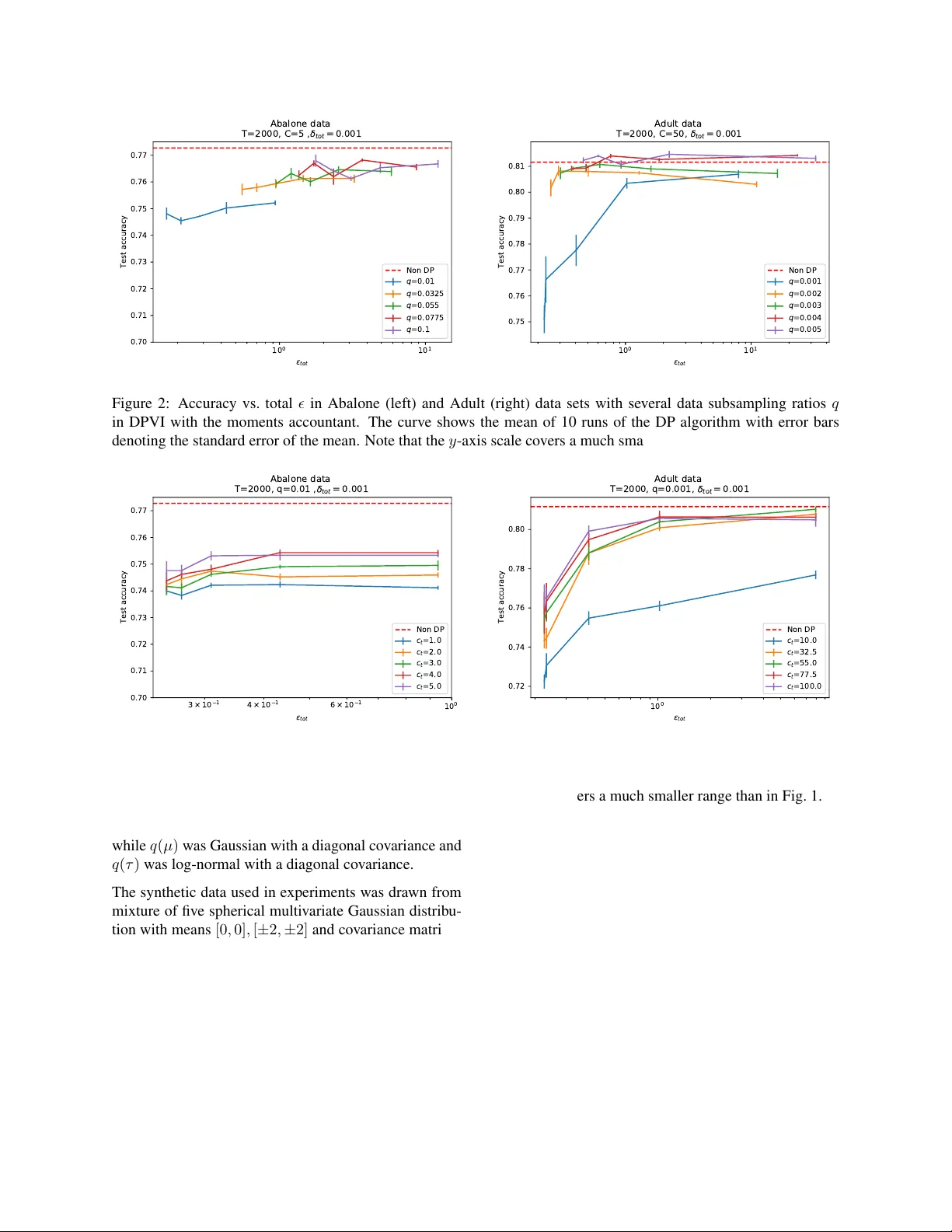
Differ entially Priv ate V ariational Infer ence f or Non-conjugate Models Joonas J ¨ alk ¨ o 1 , Onur Dikmen 1 and Antti Honkela 1 , 2 , 3 1 Helsinki Institute for Information T echnology (HIIT), Department of Computer Science 2 Department of Mathematics and Statistics 3 Department of Public Health Univ ersity of Helsinki Abstract Many machine learning applications are based on data collected from people, such as their tastes and behaviour as well as biological traits and genetic data. Regardless of how impor- tant the application might be, one has to make sure indi viduals’ identities or the priv acy of the data are not compromised in the analy- sis. Differenti al pri v acy constitutes a po wer- ful framework that pre vents breaching of data subject priv acy from the output of a com- putation. Differentially priv ate versions of many important Bayesian inference methods hav e been proposed, but there is a lack of an efficient unified approach applicable to arbi- trary models. In this contribution, we pro- pose a differentially pri v ate variational infer - ence method with a very wide applicability . It is built on top of doubly stochastic varia- tional inference, a recent advance which pro- vides a variational solution to a large class of models. W e add dif ferential priv acy into dou- bly stochastic variational inference by clipping and perturbing the gradients. The algorithm is made more efficient through priv acy amplifi- cation from subsampling. W e demonstrate the method can reach an accuracy close to non- priv ate level under reasonably strong pri v acy guarantees, clearly improving ov er previous sampling-based alternatives especially in the strong priv acy regime. 1 INTR ODUCTION Using more data usually leads to better generalisation and accurac y in machine learning. W ith more people get- ting more tightly in volved in the ubiquitous data collec- tion, pri v ac y concerns related to the data are becoming more important. People will be much more willing to contribute their data if they can be sure that the priv acy of their data can be protected. Differential priv acy (DP) (Dwork et al., 2006; Dwork and Roth, 2014) is a strong framework with strict priv ac y guarantees against attacks from adversaries with side in- formation. The main principle is that the output of an algorithm (such as a query or an estimator) should not change much if the data for one individual are modified or deleted. This can be accomplished through adding stochasticity at dif ferent levels of the estimation process, such as adding noise to data itself (input perturbation), changing the objectiv e function to be optimised or how it is optimised (objective perturbation), releasing the esti- mates after adding noise (output perturbation) or by sam- pling from a distrib ution based on utility or goodness of the alternativ es (e xponential mechanism). A lot of ground-breaking work has been done on priv ac y- preserving versions of standard machine learning ap- proaches, such as objectiv e-perturbation-based logistic regression (Chaudhuri and Monteleoni, 2008), regres- sion using functional mechanism (Zhang et al., 2012) to name a few . Pri vac y-preserving Bayesian inference (e.g. (W illiams and McSherry, 2010; Zhang et al., 2014)) has only recently started attracting more interest. The re- sult of Dimitrakakis et al. (2014) showing that the pos- terior distribution is under certain assumptions differen- tially pri vate is mathematically elegant, b ut does not lead to practically useful algorithms. Methods based on this approach suffer from the major weakness that the pri- vac y guarantees are only valid for samples drawn from the exact posterior which is usually impossible to guar- antee in practice. Methods based on perturbation of data sufficient statistics (Zhang et al., 2016; Foulds et al., 2016; Honkela et al., 2016) are asymptotically efficient, but the y are only applicable to exponential family mod- els which limits their usefulness. The sufficient statistic perturbation approach was recently also applied to vari- ational inference (Park et al., 2016), which is again ap- plicable to models where non-private inference can be performed by accessing sufficient statistics. General differentially pri v ate Bayesian inference can be realised most easily using the gradient perturba- tion mechanism. This was first proposed by W ang et al. (2015), who combine dif ferential priv acy by gra- dient perturbation with stochastic gradient Marko v chain Monte Carlo (MCMC) sampling. This approach works in principle for arbitrary models, but because of the gra- dient perturbation mechanism each MCMC iteration will consume some priv acy budget, hence sev erely limiting the number of iterations that can be run which can cause difficulties with the con ver gence of the sampler . Our goal in this work is to apply the gradient perturbation mechanism to de vise a generic dif ferentially pri v ate v ari- ational inference method. V ariational inference seems preferable to stochastic gradient MCMC here because a good optimiser should be able to make better use of the limited gradient ev aluations and the variational approx- imation provides a very efficient summary of the poste- rior . The recently proposed doubly stochastic v ariational inference T itsias and L ´ azaro-Gredilla (2014) and the fur - ther streamlined automatic differentiation variational in- ference (ADVI) method (Kucukelbir et al., 2017) provide a generic v ariational inference method also applicable to non-conjugate models. These approaches apply a series of transformations and approximations so that the v ari- ational distrib utions are Gaussian and can be optimised by stochastic gradient ascent. Here, we propose dif feren- tially pri v ate variational inference (DPVI) based on gra- dient clipping and perturbation as well as double stochas- ticity . W e make a thorough case study on the Bayesian logistic regression model with comparisons to the non- priv ate case under dif ferent design decisions for DPVI. W e also test the performance of DPVI with a Gaussian mixture model. 2 B A CKGR OUND 2.1 DIFFERENTIAL PRIV A CY Differential pri v ac y (DP) (Dwork et al., 2006; Dwork and Roth, 2014) is a framew ork that provides mathematical formulation for priv ac y that enables proving strong pri- vac y guarantees. Definition 1 (  -Dif ferential pri v ac y) . A randomised al- gorithm A is  -dif fer entially private if for all pairs of ad- jacent data sets, i.e., differing only in one data sample, x, x 0 , and for all sets S ⊂ im ( A ) Pr( A ( x ) ∈ S ) ≤ e  Pr( A ( x 0 ) ∈ S ) . There are two different variants depending on which data sets are considered adjacent: in unbounded DP data sets x, x 0 are adjacent if x 0 can be obtained from x by adding or removing an entry , while in bounded DP x, x 0 are ad- jacent if the y are of equal size and equal in all b ut one of their elements (Dwork and Roth, 2014). The definition is symmetric in x and x 0 which means that in practice the probabilities of obtaining a specific output from ei- ther algorithm need to be similar . The pri vac y parameter  measures the strength of the guarantee with smaller val- ues corresponding to stronger priv acy .  -DP defined abo ve, also known as pur e DP , is some- times too infle xible and a relaxed version called ( , δ ) - DP is often used instead. It is defined as follows: Definition 2 ( ( , δ ) -Differential priv ac y) . A randomised algorithm A is ( , δ ) -dif fer entially private if for all pairs of adjacent data sets x, x 0 and for every S ⊂ im ( A ) Pr( A ( x ) ∈ S ) ≤ e  Pr( A ( x 0 ) ∈ S ) + δ. It can be sho wn that ( , δ ) -DP provides a probabilistic  - DP guarantee with probability 1 − δ (Dw ork and Roth, 2014). 2.1.1 Gaussian mechanism There are many possibilities how to make algorithm dif- ferentially priv ate. In this paper we use objective pertur- bation . W e use the Gaussian mechanism as our method for perturbation. Dwork and Roth (2014, Theorem 3.22) state that giv en query f with ` 2 -sensitivity of ∆ 2 ( f ) , re- leasing f ( x ) + η , where η ∼ N (0 , σ 2 ) , is ( , δ ) -DP when σ 2 > 2 ln(1 . 25 /δ )∆ 2 2 ( f ) / 2 . (1) The important ` 2 -sensitivity of a query is defined as: Definition 3 ( ` 2 -sensitivity) . Given two adjacent data sets x, x 0 , ` 2 -sensitivity of query f is ∆ 2 ( f ) = sup x,x 0 || x − x 0 || =1 || f ( x ) − f ( x 0 ) || 2 . 2.1.2 Composition theorems One of the v ery useful features of DP compared to many other priv acy formulations is that it provides a very nat- ural way to study the priv acy loss incurred by repeated use of the same data set. Using an algorithm on a data set multiple times will weaken our priv acy guarantee be- cause of the potential of each application to leak more information. The DP variational inference algorithm pro- posed in this paper is iterati ve, so we need to use compo- sition theorems to bound the total priv acy loss. The simplest basic composition Dwork and Roth (2014) shows that a k -fold composition of an ( , δ ) -DP algo- rithm provides ( k , k δ ) -DP . More generally releasing joint output of k algorithms A i that are individually (  i , δ i ) -DP will be ( P k i =1  i , P k i =1 δ i ) -DP . Under pure  -DP when δ 1 = · · · = δ k = 0 this is the best known composition that yields a pure DP algorithm. Moving from the pure  -DP to general ( , δ ) -DP allows a stronger result with a smaller  at the e xpense of hav- ing a larger total δ on the composition. This trade-off is characterised by the Adv anced composition theorem of Dwork and Roth (2014, Theorem 3.20), which becomes very useful when we need to use data multiple times Theorem 1 (Adv anced composition theorem) . Given al- gorithm A that is ( , δ ) -DP and δ 0 > 0 , k -fold composi- tion of algorithm A is (  tot , δ tot ) -DP with  tot = p 2 k ln(1 /δ 0 )  + k  ( e  − 1) (2) δ tot = k δ + δ 0 . (3) The theorem states that with small loss in δ tot and with small enough  , we can provide more strict  tot than just summing the  . This is obvious by looking at the first order expansion for small  of  tot ≈ p 2 k ln(1 /δ 0 )  + k  2 . 2.1.3 Privacy amplification W e use a stochastic gradient algorithm that uses s ubsam- pled data while learning, so we can make use of the am- plifying effect of the subsampling on priv acy . This Pri- vacy amplification theor em (Li et al., 2012) states that if we run ( , δ ) -DP algorithm A on randomly sampled subset of data with uniform sampling probability q > δ , priv acy amplification theorem states that the subsampled algorithm is (  amp , δ amp ) -DP with  amp = min( , log (1 + q ( e  − 1))) (4) δ amp = q δ, (5) assuming log(1 + q ( e  − 1)) <  . 2.1.4 Moments accountant The moments accountant proposed by Abadi et al. (2016) is a method to accumulate the pri v acy cost that provides a tighter bound for  and δ than the pre vious composi- tion approaches. The moments accountant incorporates both the composition over iterations and pri v acy ampli- fication due to subsampling into a single bound gi v en by the following Theorem. Theorem 2. Ther e exist constants c 1 and c 2 so that given the sampling pr obability q = L/ N and the number of steps T , for any  < c 1 q 2 T , a DP stoc hastic gradient algorithm that clips the ` 2 norm of gradients to C and injects Gaussian noise with standard deviation 2 C σ to the gradients, is ( , δ ) -DP for any δ > 0 under bounded DP if we choose σ ≥ c 2 q p T log (2 /δ )  . (6) Pr oof. Abadi et al. (2016) sho w that injecting gradient noise with standard de viation C σ where σ satisfies the inequality (6) yields an ( , 1 2 δ ) -DP algorithm under un- bounded DP . This implies that adding noise with stan- dard de viation 2 C σ yields an ( 1 2 , 1 2 δ ) -DP algorithm un- der unbounded DP . This proves the theorem as any ( 1 2 , 1 2 δ ) unbounded DP algorithm is an ( , δ ) bounded DP algorithm. This fol- lows from the fact that the replacement of an element in the data set can be represented as a composition of one addition and one remov al of an element. Similar bounds can also be deri v ed using concentrated DP (Dwork and Rothblum, 2016; Bun and Steinke, 2016). W e use the implementation of Abadi et al. (2016) to com- pute the total  priv acy cost with a giv en δ -budget, stan- dard deviation σ of noise applied in Gaussian mechanism and subsampling ratio q . In our experiments we report results using both the ad- vanced composition theorem with priv acy amplification as well as the moments accountant. 2.2 V ARIA TIONAL B A YES V ariational Bayes (VB) methods (Jordan et al., 1999) provide a way to approximate the posterior distribution of latent variables in a model when the true posterior is intractable. True posterior p ( θ | x ) is approximated with a variational distribution q ξ ( θ ) that has a simpler form than the posterior , obtained generally by removing some dependencies from the graphical model such as the fully- factorised form q ξ ( θ ) = Q d q ξ d ( θ d ) . ξ are the vari- ational parameters and their optimal values ξ ∗ are ob- tained through minimising the Kullback-Leibler (KL) di- ver gence between q ξ ( θ ) and p ( θ | x ) . This is also equiv- alent to maximising the evidence lower bound (ELBO) L ( q ξ ) = Z q ξ ( θ ) ln  p ( D , θ ) q ξ ( θ )  = − KL ( q ξ ( θ ) || p ( θ )) + B X i =1 h ln p ( x i | θ ) i q ξ ( θ ) , where hi q ξ ( θ ) is an expectation taken w .r .t q ξ ( θ ) and the observations D = { x 1 , . . . , x N } are assumed to be ex- changeable under our model. When the model is in the conjugate e xponential family (Ghahramani and Beal, 2001) and q ξ ( θ ) is factorised, the expectations that constitute L ( q ξ ) are analytically av ail- able and each ξ d is updated iterativ ely by fixed point it- erations. Most popular applications of VB fall into this category , because handling of the more general case in- volv es more approximations, such as defining another lev el of lo wer bound to the ELBO or estimating the ex- pectations using Monte Carlo integration. 2.2.1 Doubly stochastic variational infer ence An increasingly popular alternative approach is the dou- bly stochastic variational inference framework proposed by T itsias and L ´ azaro-Gredilla (2014). The frame work is based on stochastic gradient optimisation of the ELBO. The expectation over q ξ ( θ ) is ev aluated using Monte Carlo sampling. Exchanging the order of integration (ex- pectation) and dif ferentiation and using the reparametri- sation trick to represent for example samples from a Gaussian approximation q ξ i ( θ i ) = N ( θ i ; µ i , Σ i ) as θ i = µ i + Σ 1 / 2 i z , z ∼ N (0 , I ) , it is possible to ob- tain stochastic gradients of the ELBO which can be fed to a standard stochastic gradient ascent (SGA) optimisa- tion algorithm. For models with exchangeable observ ations, the ELBO objectiv e can be brok en do wn to a sum of terms for each observation: L ( q ξ ) = − KL ( q ξ ( θ ) || p ( θ )) + N X i =1 h ln p ( x i | θ ) i q ξ ( θ ) = N X i =1  h ln p ( x i | θ ) i q ξ ( θ ) − 1 N KL ( q ξ ( θ ) || p ( θ ))  =: N X i =1 L i ( q ξ ) . This allows considering mini batches of data at each it- eration to handle big data sets, which adds another level of stochasticity to the algorithm. The recently proposed Automatic Deriv ation V ariational Inference (AD VI) framework (K ucukelbir et al., 2017) unifies different classes of models through a transforma- tion of variables and optimises the ELBO using stochas- tic gradient ascent (SGA). Constrained variables are transformed into unconstrained ones and their posterior is approximated by Gaussian variational distrib utions, which can be a product of independent Gaussians (mean- field) or larger multiv ariate Gaussians. Expectations in the gradients are approximated using Monte Carlo in- tegration and the ELBO is optimised iterativ ely using SGA. Algorithm 1 DPVI Input: Data set D , sampling probability q , number of iterations T , SGA step size η , Clipping threshold c t and initial values ξ 0 . for t ∈ [ T ] do Pick random sample U from D with sampling prob- ability q Calculate the gradient g t ( x i ) = ∇L i ( q ξ t ) for each i ∈ U Clip and sum gradients: ˜ g t ( x i ) ← g t ( x i ) / max(1 , || g t ( x i ) || 2 ) c t ) ˜ g t ← P i ˜ g t ( x i ) Add noise: ˜ g t ← ˜ g t + N (0 , 4 c 2 t σ 2 I ) Update AdaGrad parameter . G t ← G t − 1 + ˜ g 2 t Ascent: ξ t ← ξ t − 1 + η ˜ g t / √ G t end for 3 DIFFERENTIALL Y -PRIV A TE V ARIA TIONAL INFERENCE Differentially-pri vate variational inference (DPVI) is based on clipping of the contributions of individual data samples to the gradient, g t ( x i ) = ∇L i ( q ξ t ) , at each iter - ation t of the stochastic optimisation process and perturb- ing the total gradient. The algorithm is presented in Al- gorithm 1. The algorithm is very similar to the one used for deep learning by Abadi et al. (2016). DPVI can be easily implemented using automatic dif ferentiation soft- ware such as Autograd, or incorporated e ven more easily into automatic inference engines, such as the AD VI im- plementations in PyMC3 (Salv atier et al., 2016) or Ed- ward (Tran et al., 2017) which also pro vide subsampling. Each g t ( x i ) is clipped in order to calculate gradient sen- sitivity . Gradient contributions from all data samples in the mini batch are summed and perturbed with Gaussian noise N (0 , 4 c 2 t σ 2 I ) . The sampling frequency q for subsampling within the data set, total number of iterations T and the v ariance σ 2 of Gaussian noise are important design parameters that determine the priv acy cost. c t is chosen before learn- ing, and does not need to be constant. After clipping || g t ( x i ) || 2 ≤ c t , ∀ i ∈ U . Clipping gradients too much will affect accurac y , but on the other hand large clipping threshold will cause large amount of noise to sum of gra- dients. Parameter q determines ho w large subsample of the training data we use to for gradient ascent. Small q values enable pri v ac y amplification but may need a need larger T . For a very small q when the mini batches con- sist of just a few samples, the added noise will dominate ov er the gradient signal and the optimisation will fail. While in our experiments q was fixed, we could also al- ter the q during iteration. 3.1 MODELS WITH LA TENT V ARIABLES The simple approach in Algorithm 1 will not work well for models with latent variables. This is because the main gradient contrib utions to latent variables come from only a single data point, and the amount of noise that would need to be injected to mask the contribution of this point as needed by DP would make the gradient effecti vely useless. One way to deal with the problem is to take the EM al- gorithm view (Dempster et al., 1977) of latent variables as a hidden part of a larger complete data set and apply the DP protection to summaries computed from the com- plete data set. In this approach, which was also used by Park et al. (2016), no noise would be injected to the up- dates of the latent v ariables but the latent variables would nev er be released. An alternati ve potentially easier way to av oid this prob- lem is to mar ginalise out the latent v ariables if the model allows this. As the DPVI frame w ork works for arbi- trary likelihoods we can easily perform inference ev en for complicated marginalised likelihoods. This is a clear advantage over the VIPS framework of Park et al. (2016) which requires conjugate exponential f amily models. 3.2 SELECTING THE ALGORITHM HYPERP ARAMETERS The DPVI algorithm depends on a number of parameters, the most important of which are the gradient clipping threshold c t , the data subsampling ratio q and the number of iterations T . T ogether these define the total pri v ac y cost of the algorithm, b ut it is not obvious ho w to find the optimal combination of these under a fixed pri v acy budget. Unfortunately the standard machine learning hy- perparameter adaptation approach of optimising the per- formance on a validation set is not directly applicable, as ev ery test run would consume some of the priv acy bud- get. Dev eloping good heuristics for parameter tuning is thus important for practical application of the method. Out of these parameters, the subsampling ratio q seems easiest to interpret. The gradient that is perturbed in Al- gorithm 1 is a sum over q N samples in the mini batch. Similarly the standard deviation of the noise injected with the moments accountant in Eq. (6) scales linearly with q . Thus the signal-to-noise ratio for the gradients will be independent of q and q can be chosen to minimise the number of iterations T . The number of iterations T is potentially more difficult to determine as it needs to be suf ficient b ut not too lar ge. The moments accountant is somewhat forgi ving here as its pri vac y cost increases only in proportion to √ T . In practice one may need to simply pick T believ ed to be sufficiently large and hope for the best. Poor results in the end likely indicate that the number of samples in the data set may be insufficient for good results at the given lev el of pri v ac y . The gradient clipping threshold c t may be the most dif- ficult parameter to tune as that depends strongly on the details of the model. Fortunately our results do not seem ov erly sensitiv e to using the precisely optimal value of c t . Dev eloping good heuristics for choosing c t is an impor- tant objecti ve for future research. Still, the same problem is shared by e very DL method based on gradient pertur- bation including the deep learning work of Abadi et al. (2016) and the DP stochastic gradient MCMC methods of W ang et al. (2015). In the case of stochastic gradient MCMC this comes up through selecting a bound on the parameters to bound the Lipschitz constant appearing in the algorithm. A global Lipschitz constant for the ELBO would naturally translate to a c t guaranteed not to distort the gradients, but as noted by Abadi et al. (2016), it may actually be good to clip the gradients to make the method more robust against outliers. 4 EXPERIMENTS 4.1 LOGISTIC REGRESSION W e tested DPVI with two dif ferent learning tasks. Lets first consider model of logistic regression using the Abalone and Adult data sets from the UCI Machine Learning Repository (Lichman, 2013) for the binary classification task. Our model is: P ( y | x , w ) = σ ( y w T x ) p ( w ) = N ( w ; w 0 , S 0 ) , where σ ( x ) = 1 / (1 + exp( − x )) . For Abalone, individuals were divided into two classes based on whether indi vidual had less or more than 10 rings. The data set consisted of 4177 samples with 8 attributes. W e learned a posterior approximation for w using ADVI with SGA using Adagrad optimiser (Duchi et al., 2011) and sampling ratio q = 0 . 02 . The poste- rior approximation q ( w ) was Gaussian with a diagonal cov ariance. Classification was done using an additional Laplace approximation. Before training, features of the data set were normalised by subtracting feature mean and di viding by feature standard de viation. T raining was done with 80% of data. The other classification dataset “ Adult” that we used with logistic regression consisted of 48842 samples with 14 attributes. Our classification task was to predict whether or not an individual’ s annual income exceeded $50K. 1 0 1 1 0 0 1 0 1 1 0 2 t o t 0.50 0.55 0.60 0.65 0.70 0.75 Test accuracy Abalone data Non DP DP-SGLD DPVI DPVI-MA 1 0 1 1 0 0 1 0 1 1 0 2 t o t 0.55 0.60 0.65 0.70 0.75 0.80 Test accuracy Adult data Non DP DP-SGLD DPVI DPVI-MA Figure 1: Comparison of binary classification accuracies using the Abalone data set (left) and the Adult data set (right). The figure shows test set classification accuracies of non-pri v ate logistic regression, two v ariants of DPVI with the moments accountant and advanced composition accounting and DP-SGLD of W ang et al. (2015). The curv e sho ws the mean of 10 runs of both algorithms with error bars denoting the standard error of the mean. The data were preprocessed similarly as in Abalone: we subtracted the feature mean and divided by the standard deviation of each feature. W e again used 80% of the data for training the model. W e first compared the classification accuracy of models learned using two v ariants of DPVI with the moments ac- countant and advanced composition accounting as well as DP-SGLD of W ang et al. (2015). The classification results for Abalone and Adult are sho wn in Fig. 1. W e used q = 0 . 05 in Abalone corresponding to mini batches of 167 points and q = 0 . 005 in Adult corresponding to mini batches of 195 points. With Abalone the algorithm was run for 1000 iterations and with Adult for 2000 iter- ations. Clipping threshold were 5 for Abalone and 75 for Adult. Both results clearly show that e v en under comparable advanced composition accounting used by DP-SGLD, DPVI consistently yields significantly higher classification accuracy at a comparable lev el of priv ac y . Using the moments accountant further helps in obtain- ing ev en more accurate results at comparable lev el of priv acy . DPVI with the moments accountant can reach classification accuracy very close to the non-priv ate le vel already for  < 0 . 5 for both data sets. 4.1.1 The effect of algorithm hyperparameters. W e further tested ho w changing the different hyperpa- rameters of the algorithm discussed in Sec. 3.2 affects the test set classification accuracy of models learned with DPVI with the moments accountant. Fig. 2 sho ws the results when changing the data subsam- pling rate q . The result confirms the analysis of Sec. 3.2 that lar ger q tend to perform better than small q although there is a limit ho w small v alues of  can be reached with a larger q . Fig. 3 sho ws corresponding results when changing the gradient clipping threshold c t . The results clearly show that too strong clipping can hurt the accuracy signifi- cantly . Once the clipping is sufficiently mild the dif fer - ences between different options are f ar less dramatic. 4.2 GA USSIAN MIXTURE MODEL W e also tested the performance of DPVI with a Gaussian mixture model. For K components our model is π k ∼ Dir ( α ) µ ( k ) ∼ MVNormal ( 0 , I ) τ ( k ) ∼ In v-Gamma (1 , 1) with the likelihood p ( x i | π , µ , τ ) = K X k =1 π k N ( x i ; µ ( k ) , τ ( k ) I ) . Unlike standard variational inference that augments the model with indicator v ariables denoting the component responsible for generating each sample, we performed the inference directly on the mixture likelihood. This lets us avoid having to deal with latent variables that would otherwise make the DP inference more complicated. The posterior approximation q ( π , µ, τ ) = q ( π ) q ( µ ) q ( τ ) was fully factorised. q ( π ) was parametrised using soft- max transformation from a diagonal cov ariance Gaussian 1 0 0 1 0 1 t o t 0.70 0.71 0.72 0.73 0.74 0.75 0.76 0.77 Test accuracy Abalone data T = 2 0 0 0 , C = 5 , t o t = 0 . 0 0 1 Non DP q = 0 . 0 1 q = 0 . 0 3 2 5 q = 0 . 0 5 5 q = 0 . 0 7 7 5 q = 0 . 1 1 0 0 1 0 1 t o t 0.75 0.76 0.77 0.78 0.79 0.80 0.81 Test accuracy Adult data T = 2 0 0 0 , C = 5 0 , t o t = 0 . 0 0 1 Non DP q = 0 . 0 0 1 q = 0 . 0 0 2 q = 0 . 0 0 3 q = 0 . 0 0 4 q = 0 . 0 0 5 Figure 2: Accuracy vs. total  in Abalone (left) and Adult (right) data sets with several data subsampling ratios q in DPVI with the moments accountant. The curve shows the mean of 10 runs of the DP algorithm with error bars denoting the standard error of the mean. Note that the y -axis scale covers a much smaller range than in Fig. 1. 1 0 0 3 × 1 0 1 4 × 1 0 1 6 × 1 0 1 t o t 0.70 0.71 0.72 0.73 0.74 0.75 0.76 0.77 Test accuracy Abalone data T = 2 0 0 0 , q = 0 . 0 1 , t o t = 0 . 0 0 1 Non DP c t = 1 . 0 c t = 2 . 0 c t = 3 . 0 c t = 4 . 0 c t = 5 . 0 1 0 0 t o t 0.72 0.74 0.76 0.78 0.80 Test accuracy Adult data T = 2 0 0 0 , q = 0 . 0 0 1 , t o t = 0 . 0 0 1 Non DP c t = 1 0 . 0 c t = 3 2 . 5 c t = 5 5 . 0 c t = 7 7 . 5 c t = 1 0 0 . 0 Figure 3: Accuracy vs. total  in Abalone (left) and Adult (right) data sets with several gradient clipping threshold c t values in DPVI with the moments accountant. The curve sho ws the mean of 10 runs of the DP algorithm with error bars denoting the standard error of the mean. Note that the y -axis scale covers a much smaller range than in Fig. 1. while q ( µ ) w as Gaussian with a diagonal co v ariance and q ( τ ) was log-normal with a diagonal co v ariance. The synthetic data used in experiments was drawn from mixture of fi ve spherical multiv ariate Gaussian distrib u- tion with means [0 , 0] , [ ± 2 , ± 2] and cov ariance matrices I . Similar data has been used previously by Honkela et al. (2010) and Hensman et al. (2012). W e used 1000 samples from this mixture for training the model and 100 samples to test the performance. W e used both DPVI and DP-SGLD for this data. Performance comparison was done by computing the predictive likelihoods for both al- gorithms with sev eral dif ferent epsilon values. W e also show one e xample of approximate distribution that DPVI learns from abov e mixture model. From Fig. 4 we can see that DPVI algorithm performs well compared to non-pri vate v ersion of DPVI e ven with relativ ely small epsilon values. Howe ver DP-SGLD seems to outperfom DPVI when we consider more flex- ible priv acy requirements. Both DP-SGLD and DPVI used q = 0 . 003 . W e let both algorithms run for 3000 it- erations. Gradient clipping threshold for DPVI w as set to c t = 5 . W e used δ = 0 . 001 in the predictiv e likelihood comparison. For DPVI predictive likelihood was approx- imated by Monte-Carlo integration using samples from the learned approximate posterior and for DP-SGLD by using the last 100 samples the algorithm produced. Non- priv ate results were obtained by setting σ = 0 in DPVI, using q = 0 . 01 and running the algorithm for 5000 itera- tions. 1 0 1 1 0 0 1 0 1 t o t 22.5 20.0 17.5 15.0 12.5 10.0 7.5 5.0 Per Example Predictive likelihood GMM with synthetic data Non DP DP-SGLD DPVI DPVI-MA Figure 4: Per example predicti v e likelihood vs.  . For both DP-SGLD and DPVI, lines show mean between 10 runs of algorithm with error bars denoting the standard error of mean. Fig. 5 shows a visualisation of the mixture components learned by DPVI and DP-SGLD. Components inferred by DPVI appear much closer to ground truth than those from DP-SGLD. 5 DISCUSSION Our results demonstrate that the proposed DPVI method has the potential to produce very accurate learning re- sults, but this requires finding good values for algorith- mic hyperparameters that unfortunately cannot be tuned using standard approaches without compromising the priv acy . Finding good heuristics and default values for the hyperparameters is a v ery important a v enue of future research. It is tempting to think that the effect of gradient clipping would disappear as the algorithm con verges and the total gradient becomes smaller . Unfortunately this is not true as the clipping is applied on the le v el of data point spe- cific gradients which will typically not disappear ev en at con v ergence. This also means that aggressi v e clipping will change the stationary points of the SGA algorithm. One way to make the problem easier to learn under DP is to simplify it for example through dimensionality reduc- tion. This was noted for e xponential family models by Honkela et al. (2016) but the same principle carries over to DPVI too. In DPVI, lower dimensional model typi- cally has fewer parameters leading to a shorter parame- ter vector whose norm would thus be smaller, implying that smaller c t is enough. This means that simpler pos- terior approximations such as Gaussians with a diagonal cov ariance may be better under DP while without the DP constraint an approximation with a full covariance would usually be better (see also Kucukelbir et al., 2017). 6 CONCLUSIONS W e hav e introduced the DPVI method that can de- liv er differentially priv ate inference results with accuracy close to the non-priv ate doubly stochastic variational in- ference and AD VI. The method can effecti vely harness the power of AD VI to deal with very general models in- stead of just conjugate exponential models and the option of using multi variate Gaussian posterior approximations for greater accuracy . Acknowledgements This work w as funded by the Academy of Finland (Cen- tre of Excellence COIN; and grants 278300, 259440 and 283107). References M. Abadi, A. Chu, I. Goodfellow , H. B. McMahan, I. Mironov , K. T alwar , and L. Zhang. Deep learn- ing with dif ferential pri v acy . 2016. arXi v:1607.00133 [stat.ML]. M. Bun and T . Steinke. Concentrated dif ferential pri- vac y: Simplifications, e xtensions, and lower bounds. May 2016. arXiv:1605.02065 [cs.CR]. K. Chaudhuri and C. Monteleoni. Pri v acy-preserving lo- gistic re gression. In Adv . Neural Inf. Pr ocess. Syst. 21 , pages 289–296, 2008. A. P . Dempster, N. M. Laird, and D. B. Rubin. Maxi- mum likelihood from incomplete data via the em algo- rithm. J ournal of the Royal Statistical Society . Series B (Methodological) , 39(1):1–38, 1977. C. Dimitrakakis, B. Nelson, A. Mitrokotsa, and B. I. P . Rubinstein. Robust and private Bayesian inference. In ALT 2014 . 2014. J. Duchi, E. Hazan, and Y . Singer . Adapti ve subgradient methods for online learning and stochastic optimiza- tion. J. Mach. Learn. Res. , 12:2121–2159, July 2011. C. Dwork and A. Roth. The algorithmic foundations of differential priv acy . F ound. T r ends Theor . Comput. Sci. , 9(3–4):211–407, August 2014. C. Dwork and G. N. Rothblum. Concentrated dif ferential priv acy . 2016. arXiv:1603.01887 [cs.DS]. C. Dwork, F . McSherry , K. Nissim, and A. Smith. Cali- brating noise to sensiti vity in priv ate data analysis. In TCC 2006 . 2006. 10.0 7.5 5.0 2.5 0.0 2.5 5.0 7.5 10.0 6 4 2 0 2 4 6 GMM with synthetic data D P V I : M A = 0 . 2 3 , A C T = 1 . 6 9 , t o t = 0 . 0 0 1 10.0 7.5 5.0 2.5 0.0 2.5 5.0 7.5 10.0 6 4 2 0 2 4 6 GMM with synthetic data S G L D : , = 1 . 6 9 , t o t = 0 . 0 0 1 Figure 5: Approximate posterior predictive distribution for the Gaussian mixture model learned with DPVI (left) and DP-SGLD (right). The DP-SGLD distribution is formed as an av erage o ver the last 100 samples from the algorithm. J. Foulds, J. Geumlek, M. W elling, and K. Chaudhuri. On the theory and practice of priv acy-preserving Bayesian data analysis. In Pr oc. 32nd Conf. on Uncertainty in Artificial Intelligence (U AI 2016) , 2016. Z. Ghahramani and M. J. Beal. Propagation algorithms for variational Bayesian learning. In T . K. Leen, T . G. Dietterich, and V . T resp, editors, Advances in Neural Information Pr ocessing Systems 13 , pages 507–513. MIT Press, 2001. J. Hensman, M. Rattray , and N. D. Lawrence. Fast varia- tional inference in the conjugate e xponential family . In Advances in Neur al Information Pr ocessing Systems 25 , pages 2897–2905. 2012. A. Honk ela, T . Raiko, M. Kuusela, M. T ornio, and J. Karhunen. Approximate Riemannian conjugate gra- dient learning for fixed-form variational Bayes. J Mach Learn Res , 11:3235–3268, No v 2010. A. Honkela, M. Das, O. Dikmen, and S. Kaski. Ef ficient differentially priv ate learning improves drug sensitiv- ity prediction. 2016. M. I. Jordan, Z. Ghahramani, T . S. Jaakkola, and L. K. Saul. An introduction to variational methods for graphical models. Mac h. Learn. , 37(2):183–233, Nov ember 1999. A. Kucukelbir , D. T ran, R. Ranganath, A. Gelman, and D. M. Blei. Automatic dif ferentiation v ariational in- ference. J Mach Learn Res , 18(14):1–45, 2017. N. Li, W . Qardaji, and D. Su. On sampling, anonymiza- tion, and differential priv ac y or , k-anonymization meets differential priv acy . In Pr oceedings of the 7th A CM Symposium on Information, Computer and Com- munications Security , ASIA CCS ’12, pages 32–33, New Y ork, NY , USA, 2012. A CM. M. Lichman. UCI machine learning repository , 2013. URL http://archive.ics.uci.edu/ml . M. P ark, J. F oulds, K. Chaudhuri, and M. W elling. V ariational Bayes in priv ate settings (VIPS). 2016. arXiv:1611.00340 [stat.ML]. J. Salv atier , T . V . W iecki, and C. Fonnesbeck. Proba- bilistic programming in Python using PyMC3. P eerJ Computer Science , 2:e55, apr 2016. M. T itsias and M. L ´ azaro-Gredilla. Doubly stochas- tic v ariational Bayes for non-conjugate inference. In Pr oc. 31st Int. Conf . Mach. Learn. (ICML 2014) , pages 1971–1979, 2014. D. T ran, M. D. Hoffman, R. A. Saurous, E. Bre vdo, K. Murphy , and D. M. Blei. Deep probabilistic pro- gramming. In International Conference on Learning Repr esentations , 2017. Y . W ang, S. E. Fienberg, and A. J. Smola. Priv acy for free: Posterior sampling and stochastic gradient Monte Carlo. In Pr oc. 32nd Int. Conf. Mach. Learn. (ICML 2015) , pages 2493–2502, 2015. O. W illiams and F . McSherry . Probabilistic inference and differential priv ac y . In Adv . Neural Inf. Pr ocess. Syst. 23 , 2010. J. Zhang, G. Cormode, C. M. Procopiuc, D. Sriv as- tav a, and X. Xiao. PrivBayes: Priv ate data release via Bayesian networks. In SIGMOD’14 , pages 1423– 1434, 2014. J. Zhang, Z. Zhang, X. Xiao, Y . Y ang, and M. Winslett. Functional mechanism: Regression analysis under dif- ferential priv acy . PVLDB , 5(11):1364–1375, 2012. Z. Zhang, B. Rubinstein, and C. Dimitrakakis. On the differential pri v acy of Bayesian inference. In Pr oc. Conf. AAAI Artif . Intell. 2016 , 2016.