Learning Features of Music from Scratch

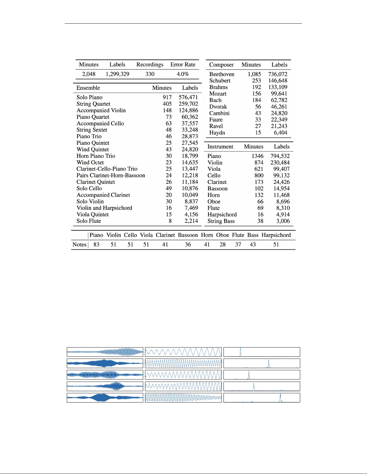
Published as a conference paper at ICLR 2017 L E A R N I N G F E A T U R E S O F M U S I C F R O M S C R A T C H John Thickstun 1 , Zaid Harchaoui 2 & Sham M. Kakade 1 , 2 1 Department of Computer Science and Engineering, 2 Department of Statistics Univ ersity of W ashington Seattle, W A 98195, USA { thickstn,sham } @cs.washington.edu , name@uw.edu A B S T R A C T This paper introduces a new lar ge-scale music dataset, MusicNet, to serve as a source of supervision and ev aluation of machine learning methods for music re- search. MusicNet consists of hundreds of freely-licensed classical music record- ings by 10 composers, written for 11 instruments, together with instrument/note annotations resulting in ov er 1 million temporal labels on 34 hours of chamber music performances under various studio and microphone conditions. The paper defines a multi-label classification task to predict notes in musical recordings, along with an ev aluation protocol, and benchmarks several machine learning architectures for this task: i) learning from spectrogram features; ii) end- to-end learning with a neural net; iii) end-to-end learning with a con volutional neural net. These experiments show that end-to-end models trained for note pre- diction learn frequency selecti ve filters as a lo w-lev el representation of audio. 1 I N T R O D U C T I O N Music research has benefited recently from the ef fecti veness of machine learning methods on a wide range of problems from music recommendation (van den Oord et al., 2013; McFee & Lanckriet, 2011) to music generation (Hadjeres & Pachet, 2016); see also the recent demos of the Google Magenta project 1 . As of today , there is no large publicly av ailable labeled dataset for the simple yet challenging task of note prediction for classical music. The MIREX MultiF0 De velopment Set (Benetos & Dixon, 2011) and the Bach10 dataset (Duan et al., 2011) together contain less than 7 minutes of labeled music. These datasets were designed for method ev aluation, not for training supervised learning methods. This situation stands in contrast to other application domains of machine learning. For instance, in computer vision lar ge labeled datasets such as ImageNet (Russako vsky et al., 2015) are fruitfully used to train end-to-end learning architectures. Learned feature representations ha ve outperformed traditional hand-crafted low-le vel visual features and lead to tremendous progress for image classi- fication. In (Humphrey et al., 2012), Humphre y , Bello, and LeCun issued a call to action: “Deep architectures often require a large amount of labeled data for supervised training, a luxury music informatics has never really enjoyed. Gi ven the proven success of supervised methods, MIR would likely benefit a good deal from a concentrated effort in the curation of sharable data in a sustainable manner . ” This paper introduces a new lar ge labeled dataset, MusicNet, which is publicly av ailable 2 as a re- source for learning feature representations of music. MusicNet is a corpus of aligned labels on freely-licensed classical music recordings, made possible by licensing initiativ es of the European Archiv e, the Isabella Stew art Gardner Museum, Musopen, and v arious indi vidual artists. The dataset consists of 34 hours of human-verified aligned recordings, containing a total of 1 , 299 , 329 individ- ual labels on segments of these recordings. T able 1 summarizes statistics of MusicNet. The focus of this paper’ s experiments is to learn low-le vel features of music from ra w audio data. In Sect. 4, we will construct a multi-label classification task to predict notes in musical recordings, 1 https://magenta.tensorflow.org/ 2 http://homes.cs.washington.edu/ ˜ thickstn/musicnet.html . 1 Published as a conference paper at ICLR 2017 MusicNet T able 1: Summary statistics of the MusicNet dataset. See Sect. 2 for further discussion of MusicNet and Sect. 3 for a description of the labelling process. Appendix A discusses the methodology for computing error rate of this process. along with an ev aluation protocol. W e will consider a variety of machine learning architectures for this task: i) learning from spectrogram features; ii) end-to-end learning with a neural net; iii) end- to-end learning with a con volutional neural net. Each of the proposed end-to-end models learns a set of frequency selecti ve filters as low-le vel features of musical audio, which are similar in spirit to a spectrogram. The learned low-le vel features are visualized in Figure 1. The learned features modestly outperform spectrogram features; we will explore possible reasons for this in Sect. 5. Figure 1: (Left) Bottom-lev el weights learned by a two-layer ReLU network trained on 16,384- samples windows ( ≈ 1 / 3 seconds) of raw audio with ` 2 regularized ( λ = 1 ) square loss for multi- label note classification on raw audio recordings. (Middle) Magnified vie w of the center of each set of weights. (Right) The truncated frequency spectrum of each set of weights. 2 Published as a conference paper at ICLR 2017 2 M U S I C N E T Related W orks. The experiments in this paper suggest that large amounts of data are necessary to reco vering useful features from music; see Sect. 4.5 for details. The Lakh dataset, released this summer based on the work of Raffel & Ellis (2015), offers note-level annotations for many 30- second clips of pop music in the Million Song Dataset (McFee et al., 2012). The syncR WC dataset is a subset of the R WC dataset (Goto et al., 2003) consisting of 61 recordings aligned to scores using the protocol described in Ewert et al. (2009). The MAPS dataset (Emiya et al., 2010) is a mixture of acoustic and synthesized data, which e xpressiv e models could o verfit. The Mazurka project 3 consists of commercial music. Access to the R WC and Mazurka datasets comes at both a cost and incon venience. Both the MAPS and Mazurka datasets are comprised entirely of piano music. The MusicNet Dataset. MusicNet is a public collection of labels (e xemplified in T able 2) for 330 freely-licensed classical music recordings of a v ariety of instruments arranged in small chamber ensembles under various studio and microphone conditions. The recordings average 6 minutes in length. The shortest recording in the dataset is 55 seconds and the longest is almost 18 minutes. T able 1 summarizes the statistics of MusicNet with breakdo wns into v arious types of labels. T able 2 demonstrates examples of labels from the MusicNet dataset. Start End Instrument Note Measure Beat Note V alue 45.29 45.49 V iolin G5 21 3 Eighth 48.99 50.13 Cello A#3 24 2 Dotted Half 82.91 83.12 V iola C5 51 2.5 Eighth T able 2: MusicNet labels on the Pascal String Quartet’ s recording of Beethoven’ s Opus 127, String Quartet No. 12 in E-flat major , I - Maestoso - Allegro. Creati ve commons use of this recording is made possible by the work of the European Archi ve. MusicNet labels come from 513 label classes using the most naive definition of a class: distinct instrument/note combinations. The breakdowns reported in T able 1 indicate the number of distinct notes that appear for each instrument in our dataset. For example, while a piano has 88 k eys only 83 of them are performed in MusicNet. For many tasks a note’ s value will be a part of its label, in which case the number of classes will expand by approximately an order of magnitude after taking the cartesian product of the set of classes with the set of values: quarter-note, eighth-note, triplet, etc. Labels regularly o verlap in the time series, creating polyphonic multi-labels. MusicNet is ske wed to wards Beethoven, thanks to the composer’ s popularity among performing ensembles. The dataset is also skewed tow ards Solo Piano due to an ab undance of digital scores av ailable for piano works. For training purposes, researchers may want to augment this dataset to increase coverage of instruments such as Flute and Oboe that are under-represented in MusicNet. Commercial recordings could be used for this purpose and labeled using the alignment protocol described in Sect. 3. 3 D A TA S E T C O N S T R U C T I O N MusicNet recordings are freely-licensed classical music collected from the European Archi ve, the Isabella Stewart Gardner Museum, Musopen, and various artists’ collections. The MusicNet la- bels are retrieved from digital MIDI scores, collected from various archiv es including the Classical Archiv es ( classicalarchives.com ) Suzuchan’ s Classic MIDI ( suzumidi.com ) and Har - feSoft ( harfesoft.de ). The methods in this section produce an alignment between a digital score and a corresponding freely-licensed recording. A recording is labeled with e vents in the score, asso- ciated to times in the performance via the alignment. Scores containing 6 , 550 , 760 additional labels are a vailable on request to researchers who wish to augment MusicNet with commercial recordings. Music-to-score alignment is a long-standing problem in the music research and signal processing communities (Raphael, 1999). Dynamic time warping (DTW) is a classical approach to this prob- lem. An early use of DTW for music alignment is Orio & Schwarz (2001) where a recording is 3 http://www.mazurka.org.uk/ 3 Published as a conference paper at ICLR 2017 aligned to a crude synthesis of its score, designed to capture some of the structure of an o vertone series. The method described in this paper aligns recordings to synthesized performances of scores, using side information from a commercial synthesizer . T o the best of our knowledge, commercial synthesis was first used for the purpose of alignment in T uretsky & Ellis (2003). The majority of pre vious work on alignment focuses on pop music. This is more challenging than aligning classical music because commercial synthesizers do a poor job reproducing the wide variety of v ocal and instrumental timbers that appear in modern pop. Furthermore, pop features inharmonic instruments such as drums for which natural metrics on frequenc y representations–including ` 2 –are not meaningful. For classical music to score alignment, a variant of the techniques described in T uretsky & Ellis (2003) works robustly . This method is described below; we discuss the ev aluation of this procedure and its error rate on MusicNet in the appendix. 0 1 0 0 2 0 0 3 0 0 4 0 0 5 0 0 6 0 0 7 0 0 8 0 0 f r a m e s ( r e c o r d i n g ) 0 1 0 0 2 0 0 3 0 0 4 0 0 5 0 0 6 0 0 f r a m e s ( sy n t h e si s) 0 1 0 0 2 0 0 3 0 0 4 0 0 5 0 0 6 0 0 7 0 0 8 0 0 f r a m e s ( r e c o r d e d p e r f o r m a n c e ) 0 5 0 1 0 0 1 5 0 2 0 0 2 5 0 sp e c t r o g r a m b i n s Figure 2: (Left) Heatmap visualization of local alignment costs between the synthesized and recorded spectrograms, with the optimal alignment path in red. The block from x = 0 to x = 100 frames corresponds to silence at the beginning of the recorded performance. The slope of the align- ment can be interpreted as an instantaneous tempo ratio between the recorded and synthesized per- formances. The curvature in the alignment between x = 100 and x = 175 corresponds to an extension of the first notes by the performer . (Right) Annotation of note onsets on the spectrogram of the recorded performance, determined by the alignment shown on the left. In order to align the performance with a score, we need to define a metric that compares short segments of the score with se gments of a performance. Musical scores can be expressed as binary vectors in E × K where E = { 1 , . . . , n } and K is a dictionary of notes. Performances reside in R T × p , where T ∈ { 1 , . . . , m } is a sequence of time steps and p is the dimensionality of the spectrogram at time T . Giv en some local cost function C : ( R p , K ) → R , a score Y ∈ E × K , and a performance X ∈ R T × p , the alignment problem is to minimize t ∈ Z n n X i =1 C ( X t i , Y i ) subject to t 0 = 0 , t n = m, t i ≤ t j if i < j . (1) Dynamic time warping gi ves an exact solution to the problem in O ( mn ) time and space. The success of dynamic time warping depends on the metric used to compare the score and the performance. Previous works can be broadly categorized into three groups that define an alignment cost C between segments of music x and score y by injecting them into a common normed space via maps Ψ and Φ : C ( x , y ) = k Ψ( x ) − Φ( y ) k (2) The most popular approach–and the one adopted by this paper–maps the score into the space of the performance (Orio & Schwarz, 2001; T uretsky & Ellis, 2003; Soulez et al., 2003). An alternati ve approach maps both the score and performance into some third space, commonly a chromogram space (Hu et al., 2003; Izmirli & Dannenberg, 2010; Joder et al., 2013). Finally , some recent methods consider alignment in score space, taking Φ = Id and learning Ψ (Garreau et al., 2014; Lajugie et al., 2016). 4 Published as a conference paper at ICLR 2017 W ith reference to the general cost (2), we must specify the maps Ψ , Φ , and the norm k · k . W e compute the cost in the performance feature space R p , hence we take Ψ = Id . F or the features, we use the log-spectrogram with a window size of 2048 samples. W e use a stride of 512 samples between features. Hence adjacent feature frames are computed with 75% overlap. For audio sampled at 44.1kHz, this results in a feature representation with 44 , 100 / 512 ≈ 86 frames per second. A discussion of these parameter choices can be found in the appendix. The map Φ is computed by a synthetizer: we used Plogue’ s Sforzando sampler together with Garritan’ s Personal Orchestra 4 sample library . For a (pseudo)-metric on R p , we take the ` 2 norm k · k 2 on the low 50 dimensions of R p . Recall that R p represents Fourier components, so we can roughly interpret the k ’th coordinate of R p as the energy associated with the frequency k × (22 , 050 / 1024) ≈ k × 22 . 5 Hz, where 22 , 050 Hz is the Nyquist frequency of a signal sampled at 44 . 1 kHz. The 50 dimension cutoff is chosen empirically: we observe that the resulting alignments are more accurate using a small number of low-frequency bins rather than the full space R p . Synthesizers do not accurately reproduce the high-frequency features of a musical instrument; by ignoring the high frequencies, we align on a part of the spectrum where the synthesis is most accurate. The proposed choice of cutof f is aggressive compared to usual settings; for instance, T uretsky & Ellis (2003) propose cutoffs in the 2 . 5 kHz range. The fundamental frequencies of many notes in MusicNet are higher than the 50 × 22 . 5 Hz ≈ 1 kHz cutoff. Nevertheless, we find that all notes align well using only the lo w-frequency information. 4 M E T H O D S W e consider identification of notes in a segment of audio x ∈ X as a multi-label classification problem, modeled as follo ws. Assign each audio se gment a binary label vector y ∈ { 0 , 1 } 128 . The 128 dimensions correspond to frequency codes for notes, and y n = 1 if note n is present at the midpoint of x . Let f : X → H indicate a feature map. W e train a multi variate linear regression to predict ˆ y given f ( x ) , which we optimize for square loss. The v ector ˆ y can be interpreted as a multi-label estimate of notes in x by choosing a threshold c and predicting label n iff ˆ y n > c . W e search for the value c that maximizes F 1 -score on a sampled subset of MusicNet. 4 . 1 R E L A T E D W O R K Learning on ra w audio is studied in both the music and speech communities. Supervised learning on music has been driv en by access to labeled datasets. Pop music labeled with chords (Harte, 2010) has lead to a long line of work on chord recognition, most recently Korzenio wsk & W idmer (2016). Genre labels and other metadata has also attracted work on representation learning, for e xample Dieleman & Schrauwen (2014). There is also substantial work modeling raw audio representations of speech; a current example is T okuda & Zen (2016). Recent work from Google DeepMind explores generativ e models of raw audio, applied to both speech and music (v an den Oord et al., 2016). The music community has worked extensi vely on a closely related problem to note prediction: fun- damental frequency estimation. This is the analysis of fundamental (in contrast to ov ertone) frequen- cies in short audio segments; these frequencies are typically considered as proxies for notes. Because access to large labeled datasets was historically limited, most of these works are unsupervised. A good ov erview of this literature can be found in Benetos et al. (2013). V ariants of non-negati ve ma- trix factorization are popular for this task; a recent example is Khlif & Sethu (2015). A dif ferent line of work models audio probabilistically , for example Ber g-Kirkpatrick et al. (2014). Recent w ork by Kelz et al. (2016) e xplores supervised models, trained using the MAPS piano dataset. 4 . 2 M U LT I - L A Y E R P E R C E P T RO N S W e build a two-layer network with features f i ( x ) = log  1 + max(0 , w T i x )  . W e find that com- pression introduced by a logarithm impro ves performance v ersus a standard ReLU netw ork (see T able 3). Figure 1 illustrates a selection of weights w i learned by the bottom layer of this network. The weights learned by the network are modulated sinusoids. This explains the effecti veness of spectrograms as a low-le vel representation of musical audio. The weights decay at the boundaries, analogous to Gabor filters in vision. This behavior is e xplained by the labeling methodology: the audio segments used here are approximately 1 / 3 of a second long, and a segment is given a note 5 Published as a conference paper at ICLR 2017 label if that note is on in the center of the segment. Therefore information at the boundaries of the segment is less useful for prediction than information nearer to the center . 4 . 3 ( L O G - ) S P E C T R O G R A M S Spectrograms are an engineered feature representation for musical audio signals, av ailable in popular software packages such as librosa (McFee et al., 2015). Spectrograms (resp. log-spectrograms) are closely related to a two-layer ReLU network (resp. the log-ReLU network described abov e). If x = ( x 1 , . . . , x t ) denotes a segment of an audio signal of length t then we can define Spec k ( x ) ≡      t − 1 X s =0 e − 2 π iks/t x s      2 = t − 1 X s =0 cos(2 π k s/t ) x s ! 2 + t − 1 X s =0 sin(2 π k s/t ) x s ! 2 . These features are not precisely learnable by a two-layer ReLU network. But recall that | x | = max(0 , x ) + max(0 , − x ) and if we take weight vectors u , v ∈ R T with u s = cos(2 π k s/t ) and v s = sin(2 π k s/t ) then the ReLU network can learn f k, cos ( x ) + f k, sin ( x ) ≡ | u T x | + | v T x | =      t − 1 X s =0 cos(2 π k s/t ) x s      +      t − 1 X s =0 sin(2 π k s/t ) x s      . W e call this family of features a ReLUgram and observe that it has a similar form to the spectrogram; we merely replace the x 7→ x 2 non-linearity of the spectrogram with x 7→ | x | . These features achiev e similar performance to spectrograms on the classification task (see T able 3). 4 . 4 W I N D OW S I Z E When we parameterize a network, we must choose the width of the set of weights in the bottom layer . This width is called the recepti ve field in the vision community; in the music community it is called the windo w size. Traditional frequency analyses, including spectrograms, are highly sensitiv e to the windo w size. W indo ws must be long enough to capture rele vant information, b ut not so long that they lose temporal resolution; this is the classical time-frequenc y tradeof f. Furthermore, windowed frequency analysis is subject to boundary effects, known as spectral leakage. Classical signal processing attempts to dampen these effects with predefined window functions, which apply a mask that attenuates the signal at the boundaries (Rabiner & Schafer, 2007). The proposed end-to-end models learn window functions. If we parameterize these models with a large windo w size then the model will learn that distant information is irrele vant to local prediction, so the magnitude of the learned weights will attenuate at the boundaries. W e therefore focus on two window sizes: 2048 samples, which captures the local content of the signal, and 16,384 samples, which is sufficient to capture almost all rele vant context (ag ain see Figure 1). 4 . 5 R E G U L A R I Z A T I O N The size of MusicNet is essential to achie ving the results in Figure 1. In Figure 3 (Left) we optimize a two-layer ReLU network on a small subset of MusicNet consisting of 65 , 000 monophonic data points. While these features do exhibit dominant frequencies, the signal is quite noisy . Comparable noisy frequency selecti ve features were recov ered by Dieleman & Schrauwen (2014); see their Fig- ure 3. W e can reco ver clean features on a small dataset using hea vy regularization, b ut this destroys classification performance; re gularizing with dropout poses a similar tradeof f. By contrast, Figure 3 (Right) shows weights learned by an unregularized two-layer network trained on the full MusicNet dataset. The models described in this paper do not overfit to MusicNet and optimal performance (reported in T able 3) is achie ved without re gularization. 4 . 6 C O N VO L U T I O N A L N E T W O R K S Previously , we estimated ˆ y by regressing against f ( x ) . W e no w consider a con volutional model that regresses against features of a collection of shifted se gments x ` near to the original segment x . The learned features of this network are visually comparable to those learned by the fully connected net- work (Figure 1). The parameters of this network are the receptive field, stride, and pooling regions. 6 Published as a conference paper at ICLR 2017 Figure 3: (Left) Features learned by a 2-layer ReLU network trained on small monophonic subset of MusicNet. (Right) Features learned by the same network, trained on the full MusicNet dataset. The results reported in T able 3 are achieved with 500 hidden units using a receptive field of 2 , 048 samples with an 8-sample stride across a window of 16 , 384 samples. These features are grouped into average pools of width 16, with a stride of 8 features between pools. A max-pooling operation yields similar results. The learned features are consistent across dif ferent parameterizations. In all cases the learned features are comparable to those of a fully connected network. 5 R E S U L T S W e hold out a test set of 3 recordings for all the results reported in this section: • Bach’ s Prelude in D major for Solo Piano. WTK Book 1, No 5. Performed by Kimiko Ishizaka. MusicNet recording id 2303. • Mozart’ s Serenade in E-flat major . K375, Movement 4 - Menuetto. Performed by the Soni V entorum W ind Quintet. MusicNet recording id 1819. • Beetho ven’ s String Quartet No. 13 in B-flat major . Opus 130, Mov ement 2 - Presto. Re- leased by the European Archiv e. MusicNet recording id 2382. The test set is a representati ve sampling of MusicNet: it co vers most of the instruments in the dataset in small, medium, and large ensembles. The test data points are e venly spaced segments separated by 512 samples, between the 1st and 91st seconds of each recording. For the wider features, there is substantial overlap between adjacent segments. Each se gment is labeled with the notes that are on in the middle of the segment. 0 . 0 0 . 2 0 . 4 0 . 6 0 . 8 1 . 0 r e c a l l 0 . 0 0 . 2 0 . 4 0 . 6 0 . 8 1 . 0 p r e c i si o n o v e r a l l o n e - n o t e t h r e e - n o t e s Figure 4: Precision-recall curv es for the con volutional network on the test set. Curves are ev al- uated on subsets of the test set consisting of all data points (blue); points with exactly one label (monophonic; green); and points with exactly three labels (red). W e ev aluate our models on three scores: precision, recall, and av erage precision. The precision score is the count of correct predictions by the model (across all data points) divided by the total number 7 Published as a conference paper at ICLR 2017 of predictions by the model. The recall score is the count of correct predictions by the model divided by the total number of (ground truth) labels in the test set. Precision and recall are parameterized by the note prediction threshold c (see Sect. 4). By varying c , we construct precision-recall curves (see Figure 4). The av erage precision score is the area under the precision-recall curve. Representation W indow Size Precision Recall A verage Precision log-spectrograms 1,024 49.0% 40.5% 39.8% spectrograms 2,048 28.9% 52.5 % 32.9% log-spectrograms 2,048 61.9% 42.0% 48.8% log-ReLUgrams 2,048 58.9% 47.9% 49.3% MLP , 500 nodes 2,048 50.1% 58.0% 52.1% MLP , 2500 nodes 2,048 53.6% 62.3% 56.2% A vgPool, 2 stride 2,148 53.4% 62.5% 56.4% log-spectrograms 8,192 64.2% 28.6% 52.1% log-spectrograms 16,384 58.4% 18.1% 45.5% MLP , 500 nodes 16,384 54.4% 64.8% 60.0% CNN, 64 stride 16,384 60.5% 71.9% 67.8% T able 3: Benchmark results on MusicNet for models discussed in this paper . The learned repre- sentations are optimized for square loss with SGD using the T ensorflo w library (Abadi et al.). W e report the precision and recall corresponding to the best F 1 -score on validation data. A spectrogram of length n is computed from 2 n samples, so the linear 1024-point spectrogram model is directly comparable to the MLP runs with 2048 raw samples. Learned features 4 modestly outperform spectrograms for comparable windo w sizes. The discussion of windowing in Sect. 4.4 partially explains this. Figure 5 suggests a second reason. Recall (Sect. 4.3) that the spectrogram features can be interpreted as the magnitude of the signal’ s inner product with sine wa ves of linearly spaced frequencies. In contrast, the proposed networks learn weights with frequencies distrib uted similarly to the distribution of notes in MusicNet (Figure 5). This giv es the network higher resolution in the most critical frequency re gions. 0 . 0 0 . 5 1 . 0 1 . 5 2 . 0 2 . 5 3 . 0 3 . 5 f r e q u e n c y ( k H z ) 0 . 0 1 0 . 0 2 0 . 0 3 0 . 0 4 0 . 0 5 0 . 0 6 0 . 0 n o t e s ( t h o u sa n d s) 0 . 0 0 . 5 1 . 0 1 . 5 2 . 0 2 . 5 3 . 0 3 . 5 f r e q u e n c y ( k H z ) 0 5 1 0 1 5 2 0 2 5 3 0 3 5 4 0 n o d e s Figure 5: (Left) The frequency distribution of notes in MusicNet. (Right) The frequency distrib ution of learned nodes in a 500-node, two-layer ReLU network. A C K N OW L E D G M E N T S W e thank Bob L. Sturm for his detailed feedback on an earlier version of the paper . W e also thank Brian McFee and Colin Raffel for fruitful discussions. Sham Kakade acknowledges funding from the W ashington Research Foundation for innov ation in Data-intensi ve Discov ery . Zaid Harchaoui acknowledges funding from the program ”Learning in Machines and Brains” of CIF AR. 4 A demonstration using learned MLP features to synthesize a musical performance is av ailable on the dataset webpage: http://homes.cs.washington.edu/ ˜ thickstn/demos.html 8 Published as a conference paper at ICLR 2017 R E F E R E N C E S M. Abadi, A. Agarw al, P . Barham, E. Brevdo, Z. Chen, C. Citro, G. Corrado, A. Davis, J. Dean, M. De vin, S. Ghemawat, I. Goodfello w , A. Harp, G. Irving, M. Isard, Y . Jia, R. Jozefo wicz, L. Kaiser, M. Kudlur , J. Lev enberg, D. Mane, R. Monga, S. Moore, D. Murray , C. Olah, M. Schus- ter , J. Shlens, B. Steiner , I. Sutsk ev er , K. T alwar , P . T ucker , V . V anhouck e, V . V asude v an, F . V ie- gas, O. V inyals, P . W arden, M. W attenberg, M. W icke, Y . Y u, and X. Zheng. T ensorFlow: Lar ge- scale machine learning on heterogeneous systems. URL http://tensorflow.org/ . E. Benetos and S. Dixon. Joint multi-pitch detection using harmonic env elope estimation for poly- phonic music transcription. IEEE Selected T opics in Signal Pr ocessing , 2011. E. Benetos, S. Dixon, D. Giannoulis, H. Kirchoff, and A. Klapuri. Automatic music transcription: challenges and future directions. Journal of Intelligent Information Systems , 2013. T . Ber g-Kirkpatrick, J. Andreas, and D. Klein. Unsupervised transcription of piano music. NIPS , 2014. S. Dieleman and B. Schrauwen. End-to-end learning for music audio. ICASSP , 2014. Z. Duan, B. Pardo, and C. Zhang. Multiple fundamental frequenc y estimation by modeling spectral peaks and non-peak regions. T ASLP , 2011. V . Emiya, R. Badeau, and B. David. Multipitch estimation of piano sounds using a ne w probabilistic spectral smoothness principle. T ASLP , 2010. S. Ewert, M. M ¨ uller , and P . Grosche. High resolution audio synchronization using chroma features. ICASSP , 2009. D. Garreau, R. Lajugie, S. Arlot, and F . Bach. Metric learning for temporal sequence alignment. NIPS , 2014. M. Goto, H. Hashiguchi, T . Nishimura, and R. Oka. R WC music database: Music genre database and musical instrument sound database. ISMIR , 2003. Ga ¨ etan Hadjeres and Franc ¸ ois Pachet. Deepbach: a steerable model for bach chorales generation. arXiv preprint , 2016. C. Harte. T owar ds Automatic Extraction of Harmony Information from Music Signals . PhD thesis, Department of Electrical Engineering, Queen Mary , Univ ersity of London, 2010. N. Hu, R. B. Dannenberg, and G. Tzanetakis. Polyphonic audio matching and alignment for music retriev al. IEEE W orkshop on Applications of Signal Processing to Audio and Acoustics , 2003. E. J. Humphrey , J. P . Bello, and Y . LeCun. Moving beyond feature design: Deep architectures and automatic feature learning in music informatics. ISMIR , 2012. O. Izmirli and R. B. Dannenberg. Understanding features and distance functions for music sequence alignment. ISMIR , 2010. C. Joder , S. Essid, and G. Richard. Learning optimal features for polyphonic audio-to-score align- ment. T ASLP , 2013. R. Kelz, M. Dorfer, F . K orzeniowski, S. B ¨ ock, A. Arzt, and G. Widmer . On the potential of simple framewise approaches to piano transcription. ISMIR , 2016. A. Khlif and V . Sethu. An iterati ve multi range non-negati ve matrix factorization algorithm for polyphonic music transcription. ISMIR , 2015. F . K orzenio wsk and G. Widmer . Feature learning for chord recognition: the deep chroma extractor . ISMIR , 2016. R. Lajugie, P . Bojanowski, P . Cuvillier , S. Arlot, and F . Bach. A weakly-supervised discriminativ e model for audio-to-score alignment. ICASSP , 2016. 9 Published as a conference paper at ICLR 2017 B. McFee and G. Lanckriet. Learning multi-modal similarity . JMLR , 2011. B. McFee, T . Bertin-Mahieux, D. P . W . Ellis, and G. Lanckriet. The million song dataset challenge. Pr oceedings of the 21st International Confer ence on W orld W ide W eb , 2012. B. McFee, C. Raffel, D. Liang, D. P . W . Ellis, M. McV icar, E. Battenberg, and O. Nieto. librosa: Audio and music signal analysis in python. SCIPY , 2015. N. Orio and D. Schwarz. Alignment of monophonic and polyphonic music to a score. International Computer Music Confer ence , 2001. G. Poliner and D. P . W . Ellis. A discriminati ve model for polyphonic piano transcription. EURASIP Journal on Applied Signal Pr ocessing , 2007. L. Rabiner and R. Schafer . Introduction to digital speech processing. F oundations and tr ends in signal pr ocessing , 2007. C. Raffel and D. P . W . Ellis. Large-scale content-based matching of MIDI and audio files. ISMIR , 2015. C. Raffel, B. McFee, E. J. Humphrey , J. Salamon, O. Nieto, D. Liang, and D. P . W . Ellis. mir e v al: A transparent implementation of common mir metrics. ISMIR , 2014. C. Raphael. Automatic segmentation of acoustic musical signals using hidden markov models. IEEE T ransactions on P attern Analysis and Machine Intelligence , 1999. O. Russakovsky , J. Deng, H. Su, J. Krause, S. Satheesh, S. Ma, Z. Huang, A. Karpathy , A. Khosla, M. Bernstein, A. C. Berg, and L. Fei-Fei. Imagenet large scale visual recognition challenge. IJCV , 2015. F . Soulez, X. Rodet, and D. Schwarz. Improving polyphonic and poly-instrumental music to score alignment. ISMIR , 2003. K. T okuda and H. Zen. Directly modeling v oiced and un voiced components in speech wav eforms by neural networks. ICASSP , 2016. R. J. T uretsky and D. P . W . Ellis. Ground-truth transcriptions of real music from force-aligned midi syntheses. ISMIR , 2003. A. van den Oord, S. Dieleman, and B. Schrauwen. Deep content-based music recommendation. NIPS , 2013. A. van den Oord, S. Dieleman, H. Zen, K. Simonyan, O. V inyals, A. Gra ves, N. Kalchbrenner , A. Senior , and K. Kavukcuoglu. W av eNet: A generativ e model for raw audio. arXiv preprint , 2016. 10 Published as a conference paper at ICLR 2017 A V A L I DA T I N G T H E M U S I C N E T L A B E L S W e validate the aligned MusicNet labels with a listening test. W e create an aural representation of an aligned score-performance pair by mixing a short sine w av e into the performance with the frequenc y indicated by the score at the time indicated by the alignment. W e can listen to this mix and, if the alignment is correct, the sine tones will exactly ov erlay the original performance; if the alignment is incorrect, the mix will sound dissonant. W e have listened to sections of each recording in the aligned dataset: the beginning, se veral ran- dom samples of middle, and the end. Mixes with substantially incorrect alignments were rejected from the dataset. Failed alignments are mostly attributable to mismatches between the midi and the recording. The most common reason for rejection is musical repeats. Classical music often contains sections with indications that they be repeated a second time; in classical music performance culture, it is often acceptable to ignore these directions. If the score and performance make different choices regarding repeats, a mismatch arises. When the score omits a repeat that occurs in the performance, the alignment typically warps o ver the entire repeated section, with correct alignments before and after . When the score includes an extra repeat, the alignment typically compresses it into very short segment, with correct alignments on either side. W e rejected alignments exhibiting either of these issues from the dataset. From the aligned performances that we deemed suf ficiently accurate to admit to the dataset, we randomly sampled 30 clips for more careful annotation and analysis. W e weighted the sample to cov er a wide cov erage of recordings with various instruments, ensemble sizes, and durations. For each sampled performance, we randomly selected a 30 second clip. Using software transforms, it is possible to slow a recording do wn to approximately 1/4 speed. T wo of the clips were too richly structured and fast to precisely analyze (slo wing the signal down any further introduces artifacts that make the signal difficult to interpret). Even in these two rejected samples, the alignments sound substantially correct. For the other 28 clips, we carefully analyzed the aligned performance mix and annotated ev ery alignment error . T w o of the authors are classically trained musicians: we independently check ed for errors and we our analyses were nearly identical. Where there was disagreement, we used the more pessimistic author’ s analysis. Over our entire set of clips we av eraged a 4 . 0% error rate. Note that we do not catch ev ery type of error . Mistaken note onsets are more easily identified than mistaken offsets. T ypically the release of one note coincides with the onset of a ne w note, which implicitly verifies the release. Howe ver , release times at the ends of phrases may be less accurate; these inaccuracies would not be co vered by our error analysis. W e were also lik ely to miss performance mistakes that maintain the meter of the performance, but for professional recordings such mistakes are rare. For stringed instruments, chords consisting of more than two notes are “rolled”; i.e. they are per- formed serially from the lowest to the highest note. Our alignment protocol cannot separate notes that are notated simultaneously in the score; a rolled chord is labeled with a single starting time, usu- ally the beginning of the first note in the roll. Therefore, there is some time period at the beginning of a roll where the top notes of the chord are labeled but have not yet occurred in the performance. There are reasonable interpretations of labeling under which these labels would be judged incorrect. On the other hand, if the labels are used to supervise transcription then ours is likely the desired labeling. W e can also qualitati vely characterize the types of errors we observ ed. The most common types of errors are anticipations and delays: a single, or small sequence of labels is aligned to a slightly early or late location in the time series. Another common source of error is missing ornaments and trills: these are short flourishes in a performance are sometimes not annotated in our score data, which results in a missing annotation in the alignment. Finally , there are rare performance errors in the recordings and transcription errors in the score. 11 Published as a conference paper at ICLR 2017 B A L I G N M E N T P A R A M E T E R R O B U S T N E S S The definitions of audio featurization and the alignment cost function were contingent on several parameter choices. These choices were optimized by systematic exploration of the parameter space. W e in vestigated what happens as we vary each parameter and made the choices that gav e the best results in our listening tests. Fine-tuning of the parameters yields marginal gains. The quality of alignments improves uniformly with the quality of synthesis. The time-resolution of labels improves uniformly as the stride parameter decreases; minimization of stride is limited by system memory constraints. W e find that the precise phase-inv ariant feature specification has little effect on alignment quality . W e experimented with spectrograms and log-spectrograms using windowed and un-windo wed signals. Alignment quality seemed to be largely unaffected. The other parameters are governed by a tradeof f curve; the optimal choice is determined by balanc- ing desirable outcomes. The F ourier windo w size is a classic tradeoff between time and frequency resolution. The ` 2 norm can be understood as a tradeoff between the e xtremes of ` 1 and ` ∞ . The ` 1 norm is too egalitarian: the preponderance of errors due to synthesis quality add up and overwhelm the signal. On the other hand, the ` ∞ norm ignores too much of the signal in the spectrogram. The spectrogram cutoff, discussed in Sec. 3, is also a tradeoff between synthesis quality and maximal use of information C A D D I T I O N A L E R R O R A N A L Y S I S For each model, using the test set described in Sect. 5, we report accuracy and error scores used by the MIR community to ev aluate the Multi-F0 systems. Definitions and a discussion of these metrics are presented in Poliner & Ellis (2007). Representation Acc Etot Esub Emiss Efa 512-point log-spectrogram 28.5% .819 .198 .397 .224 1024-point log-spectrogram 33.4% .715 .123 .457 .135 1024-point log-ReLUgram 35.9% .711 .144 .377 .190 4096-point log-spectrogram 24.7% .788 .085 .628 .074 8192-point log-spectrogram 16.1% .866 .082 .737 .047 MLP , 500 nodes, 2048 raw samples 36.8% .790 .206 .214 .370 MLP , 2500 nodes. 2048 samples 40.4% .740 .177 .200 .363 A vgPool, 5 stride, 2048 samples 40.5% .744 .176 .200 .369 MLP , 500 nodes, 16384 samples 42.0% .735 .160 .191 .383 CNN, 64 stride, 16384 samples 48.9% .634 .117 .164 .352 T able 4: MIREX-style statistics, e valuated using the mir e val library (Raf fel et al., 2014). 12 Published as a conference paper at ICLR 2017 D P R E C I S I O N & R E C A L L C U RV E S 0 . 0 0 . 2 0 . 4 0 . 6 0 . 8 1 . 0 r e c a l l 0 . 0 0 . 2 0 . 4 0 . 6 0 . 8 1 . 0 p r e c i si o n Figure 6: The linear spectrogram model. 0 . 0 0 . 2 0 . 4 0 . 6 0 . 8 1 . 0 r e c a l l 0 . 0 0 . 2 0 . 4 0 . 6 0 . 8 1 . 0 p r e c i si o n Figure 7: The 500 node, 2048 raw sample MLP . 0 . 0 0 . 2 0 . 4 0 . 6 0 . 8 1 . 0 r e c a l l 0 . 0 0 . 2 0 . 4 0 . 6 0 . 8 1 . 0 p r e c i si o n Figure 8: The 2500 node, 2048 raw sample MLP . 0 . 0 0 . 2 0 . 4 0 . 6 0 . 8 1 . 0 r e c a l l 0 . 0 0 . 2 0 . 4 0 . 6 0 . 8 1 . 0 p r e c i si o n Figure 9: The av erage pooling model. 0 . 0 0 . 2 0 . 4 0 . 6 0 . 8 1 . 0 r e c a l l 0 . 0 0 . 2 0 . 4 0 . 6 0 . 8 1 . 0 p r e c i si o n Figure 10: The 500 node, 16384 raw sample MLP . 0 . 0 0 . 2 0 . 4 0 . 6 0 . 8 1 . 0 r e c a l l 0 . 0 0 . 2 0 . 4 0 . 6 0 . 8 1 . 0 p r e c i si o n Figure 11: The con volutional model. 13 Published as a conference paper at ICLR 2017 E A D D I T I O N A L R E S U LT S W e report additional results on splits of the test set described in Sect. 5. Model Features Precision Recall A verage Precision MLP , 500 nodes 2048 ra w samples 56.1% 62.7% 59.2% MLP , 2500 nodes 2048 raw samples 59.1% 67.8% 63.1% A vgPool, 5 stride 2048 raw samples 59.1% 68.2% 64.5% MLP , 500 nodes 16384 ra w samples 60.2% 65.2% 65.8% CNN, 64 stride 16384 raw samples 65.9% 75.2% 74.4% T able 5: The Soni V entorum recording of Mozart’ s Wind Quintet K375 (MusicNet id 1819). Model Features Precision Recall A verage Precision MLP , 500 nodes 2048 ra w samples 35.4% 40.7% 28.0% MLP , 2500 nodes 2048 raw samples 38.3% 44.3% 30.9% A vgPool, 5 stride 2048 raw samples 38.6% 45.2% 31.7% MLP , 500 nodes 16384 ra w samples 43.4% 51.3% 41.0% CNN, 64 stride 16384 raw samples 51.0% 57.9% 49.3% T able 6: The European Archiv e recording of Beethov en’ s String Quartet No. 13 (MusicNet id 2382). Model Features Precision Recall A verage Precision MLP , 500 nodes 2048 ra w samples 55.6% 67.4% 64.1% MLP , 2500 nodes 2048 raw samples 60.1% 71.3% 68.6% A vgPool, 5 stride 2048 raw samples 59.6% 70.7% 68.1% MLP , 500 nodes 16384 ra w samples 57.1% 76.3% 68.4% CNN, 64 stride 16384 raw samples 61.9% 80.1% 73.9% T able 7: The Kimiko Ishizaka recording of Bach’ s Prelude in D major (MusicNet id 2303). 14