Safe Exploration in Finite Markov Decision Processes with Gaussian Processes

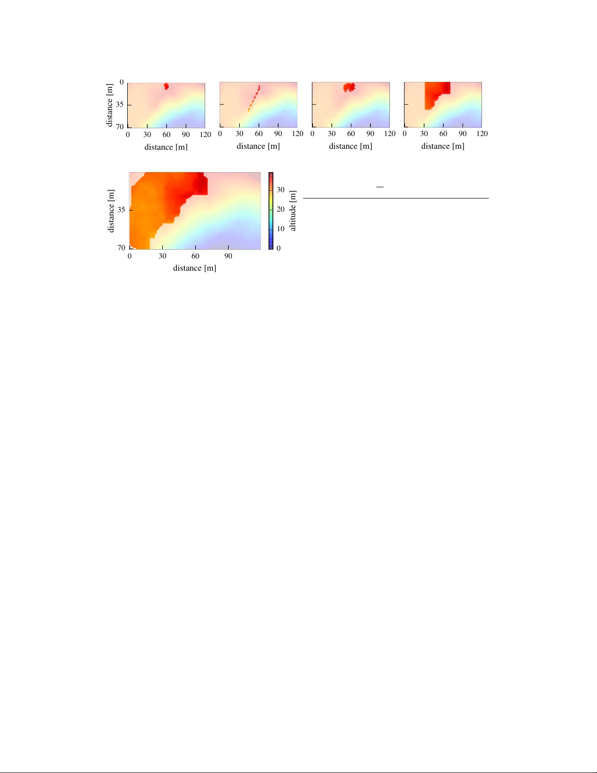
Safe Exploration in Finite Mark ov Decision Pr ocesses with Gaussian Pr ocesses Matteo T urchetta ETH Zurich matteotu@ethz.ch Felix Berk enkamp ETH Zurich befelix@ethz.ch Andreas Krause ETH Zurich krausea@ethz.ch Abstract In classical reinforcement learning agents accept arbitrary short term loss for long term gain when e xploring their en vironment. This is infeasible for safety critical applications such as robotics, where even a single unsafe action may cause system failure or harm the en vironment. In this paper , we address the problem of safely exploring finite Marko v decision processes (MDP). W e define safety in terms of an a priori unknown safety constraint that depends on states and actions and satisfies certain regularity conditions expressed via a Gaussian process prior . W e de velop a nov el algorithm, S A F E M D P , for this task and prove that it completely explores the safely reachable part of the MDP without violating the safety constraint. T o achie ve this, it cautiously explores safe states and actions in order to gain statistical confidence about the safety of un visited state-action pairs from noisy observations collected while navigating the en vironment. Moreov er, the algorithm explicitly considers reachability when exploring the MDP , ensuring that it does not get stuck in any state with no safe way out. W e demonstrate our method on digital terrain models for the task of exploring an unkno wn map with a rover . 1 Introduction T oday’ s robots are required to operate in v ariable and often unkno wn environments. The traditional solution is to specify all potential scenarios that a robot may encounter during operation a priori . This is time consuming or ev en infeasible. As a consequence, robots need to be able to learn and adapt to unkno wn en vironments autonomously [ 10 , 2 ]. While exploration algorithms are known, safety is still an open problem in the dev elopment of such systems [ 18 ]. In fact, most learning algorithms allo w robots to make unsafe decisions during exploration. This can damage the platform or its en vironment. In this paper , we provide a solution to this problem and de velop an algorithm that enables agents to safely and autonomously explore unkno wn en vironments. Specifically , we consider the problem of exploring a Mark ov decision process (MDP), where it is a priori unkno wn which state-action pairs are safe. Our algorithm cautiously explores this en vironment without taking actions that are unsafe or may render the exploring agent stuck. Related W ork. Safe exploration is an open problem in the reinforcement learning community and sev eral definitions of safety hav e been proposed [ 16 ]. In risk-sensiti ve reinforcement learning, the goal is to maximize the expected return for the worst case scenario [ 5 ]. Howe ver , these approaches only minimize risk and do not treat safety as a hard constraint. For example, Geibel and W ysotzki [7] define risk as the probability of dri ving the system to a pre viously known set of undesirable states. The main difference to our approach is that we do not assume the undesirable states to be known a priori . Garcia and Fernández [6] propose to ensure safety by means of a backup policy; that is, a policy that is known to be safe in advance. Our approach is different, since it does not require a backup policy b ut only a set of initially safe states from which the agent starts to explore. Another approach that makes use of a backup polic y is shown by Hans et al. [9] , where safety is defined in terms of a minimum rew ard, which is learned from data. 29th Conference on Neural Information Processing Systems (NIPS 2016), Barcelona, Spain. Moldov an and Abbeel [14] provide probabilistic safety guarantees at e very time step by optimizing ov er ergodic policies; that is, policies that let the agent recover from an y visited state. This approach needs to solve a large linear program at e very time step, which is computationally demanding e ven for small state spaces. Nevertheless, the idea of er godicity also plays an important role in our method. In the control community , safety is mostly considered in terms of stability or constraint satisfaction of controlled systems. Akametalu et al. [1] use reachability analysis to ensure stability under the assumption of bounded disturbances. The work in [ 3 ] uses robust control techniques in order to ensure robust stability for model uncertainties, while the uncertain model is impro ved. Another field that has recently considered safety is Bayesian optimization [ 13 ]. There, in order to find the global optimum of an a priori unknown function [ 21 ], regularity assumptions in form of a Gaussian process (GP) [ 17 ] prior are made. The corresponding GP posterior distrib ution over the unknown function is used to guide ev aluations to informative locations. In this setting, safety centered approaches include the work of Sui et al. [22] and Schreiter et al. [20] , where the goal is to find the safely reachable optimum without violating an a priori unkno wn safety constraint at any ev aluation. T o achiev e this, the function is cautiously explored, starting from a set of points that is known to be safe initially . The method in [ 22 ] was applied to the field of robotics to safely optimize the controller parameters of a quadrotor vehicle [ 4 ]. Howe ver , they considered a bandit setting, where at each iteration an y arm can be played. In contrast, we consider exploring an MDP , which introduces restrictions in terms of reachability that hav e not been considered in Bayesian optimization before. Contribution. W e introduce S A F E M D P , a novel algorithm for safe exploration in MDPs. W e model safety via an a priori unknown constraint that depends on state-action pairs. Starting from an initial set of states and actions that are known to satisfy the safety constraint, the algorithm exploits the regularity assumptions on the constraint function in order to determine if nearby , un visited states are safe. This leads to safe exploration, where only state-actions pairs that are known to fulfil the safety constraint are ev aluated. The main contribution consists of extending the work on safe Bayesian optimization in [ 22 ] from the bandit setting to deterministic, finite MDPs. In order to achie ve this, we explicitly consider not only the safety constraint, b ut also the reachability properties induced by the MDP dynamics. W e provide a full theoretical analysis of the algorithm. It prov ably enjoys similar safety guarantees in terms of ergodicity as discussed in [ 14 ], but at a reduced computational cost. The reason for this is that our method separates safety from the reachability properties of the MDP . Beyond this, we prove that S A F E M D P is able to fully explore the safely reachable region of the MDP , without getting stuck or violating the safety constraint with high probability . T o the best of our knokwledge, this is the first full exploration result in MDPs subject to a safety constraint. W e validate our method on an e xploration task, where a rover has to e xplore an a priori unknown map. 2 Problem Statement In this section, we define our problem and assumptions. The unknown en vironment is modeled as a finite, deterministic MDP [ 23 ]. Such a MDP is a tuple hS , A ( · ) , f ( s , a ) , r ( s , a ) i with a finite set of states S , a set of state-dependent actions A ( · ) , a kno wn, deterministic transition model f ( s , a ) , and rew ard function r ( s , a ) . In the typical reinforcement learning framework, the goal is to maximize the cumulativ e reward. In this paper, we consider the problem of safely exploring the MDP . Thus, instead of aiming to maximize the cumulati ve rewards, we define r ( s , a ) as an a priori unknown safety feature. Although r ( s , a ) is unkno wn, we make regularity assumptions about it to make the problem tractable. When trav ersing the MDP , at each discrete time step, k , the agent has to decide which action and thereby state to visit next. W e assume that the underlying system is safety-critical and that for any visited state-action pair , ( s k , a k ) , the unkno wn, associated safety feature, r ( s k , a k ) , must be abov e a safety threshold, h . While the assumption of deterministic dynamics does not hold for general MDPs, in our framework, uncertainty about the en vironment is captured by the safety feature. If requested, the agent can obtain noisy measurements of the safety feature, r ( s k , a k ) , by taking action a k in state s k . The index t is used to index measurements, while k denotes mov ement steps. T ypically k  t . It is hopeless to achiev e the goal of safe exploration unless the agent starts in a safe location. Hence, we assume that the agent stays in an initial set of state action pairs, S 0 , that is known to be safe a priori . The goal is to identify the maximum safely reachable re gion starting from S 0 , without visiting any unsafe states. For clarity of e xposition, we assume that safety depends on states only; that is, r ( s , a ) = r ( s ) . W e provide an e xtension to safety features that also depend on actions in Fig. 2b. 2 Figure 1: Illustration of the set operators with S = { ¯ s 1 , ¯ s 2 } . The set S = { s } can be reached from s 2 in one step and from s 1 in two steps, while only the state s 1 can be reached from s . V isiting s 1 is safe; that is, it is abov e the safety threshold, is reachable, and there exists a safe return path through s 2 . Assumptions on the reward function Ensuring that all visited states are safe without an y prior knowledge about the safety feature is an impossible task (e.g., if the safety feature is discontinuous). Howe ver , many practical safety features exhibit some regularity , where similar states will lead to similar values of r . In the following, we assume that S is endowed with a positi ve definite kernel function k ( · , · ) and that the function r ( · ) has bounded norm in the associated Reproducing K ernel Hilbert Space (RKHS) [ 19 ]. The norm induced by the inner product of the RKHS indicates the smoothness of functions with re- spect to the k ernel. This assumption allo ws us to model r as a GP [ 21 ], r ( s ) ∼ G P ( µ ( s ) , k ( s , s 0 )) . A GP is a probability distribution over functions that is fully specified by its mean function µ ( s ) and its covariance function k ( s , s 0 ) . The randomness expressed by this distribution captures our uncertainty about the en vironment. W e assume µ ( s ) = 0 for all s ∈ S , without loss of generality . The posterior distribution over r ( · ) can be computed analytically , based on t mea- surements at states D t = { s 1 , . . . , s t } ⊆ S with measurements, y t = [ r ( s 1 ) + ω 1 . . . r ( s t ) + ω t ] T , that are corrupted by zero-mean Gaussian noise, ω t ∼ N (0 , σ 2 ) . The posterior is a G P distribution with mean µ t ( s ) = k t ( s ) T ( K t + σ 2 I ) − 1 y t , variance σ t ( s ) = k t ( s , s ) , and cov ari- ance k t ( s , s 0 ) = k ( s , s 0 ) − k t ( s ) T ( K t + σ 2 I ) − 1 k t ( s 0 ) , where k t ( s ) = [ k ( s 1 , s ) , . . . , k ( s t , s )] T and K t is the positi ve definite kernel matrix, [ k ( s , s 0 )] s , s 0 ∈ D t . The identity matrix is denoted by I ∈ R t × t . W e also assume L -Lipschitz continuity of the safety function with respect to some metric d ( · , · ) on S . This is guaranteed by many commonly used kernels with high probability [21, 8]. Goal In this section, we define the goal of safe e xploration. In particular, we ask what the best that any algorithm may hope to achiev e is. Since we only observe noisy measurements, it is impossible to know the underlying safety function r ( · ) exactly after a finite number of measurements. Instead, we consider algorithms that only ha ve knowledge of r ( · ) up to some statistical confidence  . Based on this confidence within some safe set S , states with small distance to S can be classified to satisfy the safety constraint using the Lipschitz continuity of r ( · ) . The resulting set of safe states is R safe  ( S ) = S ∪ { s ∈ S | ∃ s 0 ∈ S : r ( s 0 ) −  − Ld ( s , s 0 ) ≥ h } , (1) which contains states that can be classified as safe given the information about the states in S . While (1) considers the safety constraint, it does not consider any restrictions put in place by the structure of the MDP . In particular , we may not be able to visit e very state in R safe  ( S ) without visiting an unsafe state first. As a result, the agent is further restricted to R reach ( S ) = S ∪ { s ∈ S | ∃ s 0 ∈ S, a ∈ A ( s 0 ) : s = f ( s 0 , a ) } , (2) the set of all states that can be reached starting from the safe set in one step. These states are called the one-step safely reachable states. Ho wev er, e ven restricted to this set, the agent may still get stuck in a state without any safe actions. W e define R ret ( S, S ) = S ∪ { s ∈ S | ∃ a ∈ A ( s ) : f ( s , a ) ∈ S } (3) as the set of states that are able to return to a set S through some other set of states, S , in one step. In particular , we care about the ability to return to a certain set through a set of safe states S . Therefore, these are called the one-step safely returnable states. In general, the return routes may require taking more than one action, see Fig. 1. The n -step returnability operator R ret n ( S, S ) = R ret ( S, R ret n − 1 ( S, S )) with R ret 1 ( S, S ) = R ret ( S, S ) considers these longer return routes by repeatedly applying the return operator , R ret in (3), n times. The limit R ret ( S, S ) = lim n →∞ R ret n ( S, S ) contains all the states that can reach the set S through an arbitrarily long path in S . 3 Algorithm 1 Safe exploration in MDPs ( SafeMDP) Inputs: states S , actions A , transition function f ( s , a ) , kernel k ( s , s 0 ) , Safety threshold h , Lipschitz constant L , Safe seed S 0 . C 0 ( s ) ← [ h, ∞ ) for all s ∈ S 0 for t = 1 , 2 , . . . do S t ← { s ∈ S | ∃ s 0 ∈ ˆ S t − 1 : l t ( s 0 ) − Ld ( s , s 0 ) ≥ h } ˆ S t ← { s ∈ S t | s ∈ R reach ( ˆ S t − 1 ) , s ∈ R ret ( S t , ˆ S t − 1 ) } G t ← { s ∈ ˆ S t | g t ( s ) > 0 } s t ← argmax s ∈ G t w t ( s ) Safe Dijkstra in S t from s t − 1 to s t Update GP with s t and y t ← r ( s t ) + ω t if G t = ∅ or max s ∈ G t w t ( s ) ≤  then Break For safe e xploration of MDPs, all of the above are requirements; that is, an y state that we may want to visit needs to be safe (satisfy the safety constraint), reachable, and we must be able to return to safe states from this new state. Thus, any algorithm that aims to safely explore an MDP is only allo wed to visit states in R  ( S ) = R safe  ( S ) ∩ R reach ( S ) ∩ R ret ( R safe  ( S ) , S ) , (4) which is the intersection of the three safety-relev ant sets. Gi ven a safe set S that fulfills the safety requirements, R ret ( R safe  ( S ) , S ) is the set of states from which we can return to S by only visiting states that can be classified as abov e the safety threshold. By including it in the definition of R  ( S ) , we av oid the agent getting stuck in a state without an action that leads to another safe state to take. Giv en knowledge about the safety feature in S up to  accuracy thus allo ws us to expand the set of safe ergodic states to R  ( S ) . Any algorithm that has the goal of exploring the state space should consequently explore these newly av ailable safe states and gain new knowledge about the safety feature to potentially further enlargen the safe set. The safe set after n such expansions can be found by repeatedly applying the operator in (4): R n  ( S ) = R  ( R n − 1  ( S )) with R 1  = R  ( S ) . Ultimately , the size of the safe set is bounded by surrounding unsafe states or the number of states in S . As a result, the biggest set that an y algorithm may classify as safe without visiting unsafe states is gi ven by taking the limit, R  ( S ) = lim n →∞ R n  ( S ) . Thus, given a tolerance lev el  and an initial safe seed set S 0 , R  ( S 0 ) is the set of states that any algorithm may hope to classify as safe. Let S t denote the set of states that an algorithm determines to be safe at iteration t . In the following, we will refer to complete, safe exploration whenev er an algorithm fulfills R  ( S 0 ) ⊆ lim t →∞ S t ⊆ R 0 ( S 0 ) ; that is, the algorithm classifies e very safely reachable state up to  accuracy as safe, without misclassification or visiting unsafe states. 3 S A F E M D P Algorithm W e start by giving a high le vel overvie w of the method. The S A F E M D P algorithm relies on a GP model of r to make predictions about the safety feature and uses the predicti ve uncertainty to guide the safe exploration. In order to guarantee safety , it maintains two sets. The first set, S t , contains all states that can be classified as satisfying the safety constraint using the GP posterior, while the second one, ˆ S t , additionally considers the ability to reach points in S t and the ability to safely return to the previous safe set, ˆ S t − 1 . The algorithm ensures safety and ergodicity by only visiting states in ˆ S t . In order to expand the safe region, the algorithm visits states in G t ⊆ ˆ S t , a set of candidate states that, if visited, could expand the safe set. Specifically , the algorithm selects the most uncertain state in G t , which is the safe state that we can gain the most information about. W e move to this state via the shortest safe path, which is guaranteed to exist (Lemma 2). The algorithm is summarized in Algorithm 1. Initialization. The algorithm relies on an initial safe set S 0 as a starting point to e xplore the MDP . These states must be safe; that is, r ( s ) ≥ h , for all s ∈ S 0 . They must also fulfill the reachability and returnability requirements from Sec. 2. Consequently , for any two states, s , s 0 ∈ S 0 , there must exist a path in S 0 that connects them: s 0 ∈ R ret ( S 0 , { s } ) . While this may seem restricti ve, the requirement is, for example, fulfilled by a single state with an action that leads back to the same state. 4 s 0 s 2 s 4 s 6 s 8 s 10 s 12 s 14 s 16 s 18 Safety r ( s ) (a) States are classified as safe (abov e the safety con- straint, dashed line) according to the confidence in- tervals of the GP model (red bar). States in the green bar can expand the safe set if sampled, G t . (b) Modified MDP model that is used to encode safety features that depend on actions. In this model, actions lead to abstract action-states s a , which only have one av ailable action that leads to f ( s , a ) . Classification. In order to safely explore the MDP , the algorithm must determine which states are safe without visiting them. The regularity assumptions introduced in Sec. 2 allow us to model the safety feature as a G P , so that we can use the uncertainty estimate of the GP model in order to determine a confidence interval within which the true safety function lies with high probability . For ev ery state s , this confidence interval has the form Q t ( s ) =  µ t − 1 ( s ) ± √ β t σ t − 1 ( s )  , where β t is a positiv e scalar that determines the amplitude of the interval. W e discuss ho w to select β t in Sec. 4. Rather than defining high probability bounds on the v alues of r ( s ) directly in terms of Q t , we consider the intersection of the sets Q t up to iteration t , C t ( s ) = Q t ( s ) ∩ C t − 1 ( s ) with C 0 ( s ) = [ h, ∞ ] for safe states s ∈ S 0 and C 0 ( s ) = R otherwise. This choice ensures that set of states that we classify as safe does not shrink o ver iterations and is justified by the selection of β t in Sec. 4. Based on these con- fidence interv als, we define a lo wer bound, l t ( s ) = min C t ( s ) , and upper bound, u t ( s ) = max C t ( s ) , on the v alues that the safety features r ( s ) are likely to take based on the data obtained up to iteration t . Based on these lower bounds, we define S t =  s ∈ S | ∃ s 0 ∈ ˆ S t − 1 : l t ( s 0 ) − Ld ( s , s 0 ) ≥ h  (5) as the set of states that fulfill the safety constraint on r with high probability by using the Lipschitz constant to generalize beyond the current safe set. Based on this classification, the set of ergodic safe states is the set of states that achiev e the safety threshold and, additionally , fulfill the reachability and returnability properties discussed in Sec. 2: ˆ S t =  s ∈ S t | s ∈ R reach ( ˆ S t − 1 ) ∩ R ret ( S t , ˆ S t − 1 )  . (6) Expanders. W ith the set of safe states defined, the task of the algorithm is to identify and e xplore states that might e xpand the set of states that can be classified as safe. W e use the uncertainty estimate in the GP in order to define an optimistic set of expanders, G t = { s ∈ ˆ S t | g t ( s ) > 0 } , (7) where g t ( s ) =   { s 0 ∈ S \ S t | u t ( s ) − Ld ( s , s 0 ) ≥ h }   . The function g t ( s ) is positiv e whenev er an optimistic measurement at s , equal to the upper confidence bound, u t ( s ) , would allow us to determine that a pre viously unsafe state indeed has v alue r ( s 0 ) abov e the safety threshold. Intuitively , sampling s might lead to the e xpansion of S t and thereby ˆ S t . The set G t explicitly considers the expansion of the safe set as exploration goal, see Fig. 2a for a graphical illustration of the set. Sampling and shortest safe path. The remaining part of the algorithm is concerned with selecting safe states to ev aluate and finding a safe path in the MDP that leads towards them. The goal is to visit states that allow the safe set to expand as quickly as possible, so that we do not waste resources when exploring the MDP . W e use the GP posterior uncertainty about the states in G t in order to make this choice. At each iteration t , we select as next target sample the state with the highest variance in G t , s t = argmax s ∈ G t w t ( s ) , where w t ( s ) = u t ( s ) − l t ( s ) . This choice is justified, because while all points in G t are safe and can potentially enlarge the safe set, based on one noisy sample we can gain the most information from the state that we are the most uncertain about. This design choice maximizes the knowledge acquired with ev ery sample but can lead to long paths between measurements within the safe region. Giv en s t , we use Dijkstra’ s algorithm within the set ˆ S t in order to find the shortest safe path to the target from the current state, s t − 1 . Since we require reachability and returnability for all safe states, such a path is guaranteed to exist. W e terminate the algorithm when we reach the desired accuracy; that is, argmax s ∈ G t w t ( s ) ≤  . Action-dependent safety . So far , we hav e considered safety features that only depend on the states, r ( s ) . In general, safety can also depend on the actions, r ( s , a ) . In this section, we introduce a 5 modified MDP that captures these dependencies without modifying the algorithm. The modified MDP is equivalent to the original one in terms of dynamics, f ( s , a ) . Howe ver , we introduce additional action-states s a for each action in the original MDP . When we start in a state s and take action a , we first transition to the corresponding action-state and from there transition to f ( s , a ) deterministically . This model is illustrated in Fig. 2b. Safety features that depend on action-states, s a , are equi valent to action-dependent safety features. The S A F E M D P algorithm can be used on this modified MDP without modification. See the experiments in Sec. 5 for an e xample. 4 Theoretical Results The safety and exploration aspects of the algorithm that we presented in the previous section rely on the correctness of the confidence intervals C t ( s ) . In particular , they require that the true value of the safety feature, r ( s ) , lies within C t ( s ) with high probability for all s ∈ S and all iterations t > 0 . Furthermore, these confidence intervals ha ve to shrink sufficiently fast over time. The probability of r taking values within the confidence intervals depends on the scaling factor β t . This scaling factor trades of f conservati veness in the exploration for the probability of unsafe states being visited. Appropriate selection of β t has been studied by Sriniv as et al. [21] in the multi-armed bandit setting. Even though our frame work is different, their setting can be applied to our case. W e choose, β t = 2 B + 300 γ t log 3 ( t/δ ) , (8) where B is the bound on the RKHS norm of the function r ( · ) , δ is the probability of visiting unsafe states, and γ t is the maximum mutual information that can be gained about r ( · ) from t noisy observations; that is, γ t = max | A |≤ t I ( r, y A ) . The information capacity γ t has a sublinear dependence on t for many commonly used kernels [ 21 ]. The choice of β t in (8) is justified by the following Lemma, which follo ws from [21, Theorem 6]: Lemma 1. Assume that k r k 2 k ≤ B , and that the noise ω t is zer o-mean conditioned on the history , as well as uniformly bounded by σ for all t > 0 . If β t is chosen as in (8) , then, for all t > 0 and all s ∈ S , it holds with pr obability at least 1 − δ that r ( s ) ∈ C t ( s ) . This Lemma states that, for β t as in (8), the safety function r ( s ) takes v alues within the confidence interv als C ( s ) with high probability . Now we sho w that the the safe shortest path problem has al ways a solution: Lemma 2. Assume that S 0 6 = ∅ and that for all states, s , s 0 ∈ S 0 , s ∈ R ret ( S 0 , { s 0 } ) . Then, when using Algorithm 1 under the assumptions in Theorem 1, for all t > 0 and for all states, s , s 0 ∈ ˆ S t , s ∈ R ret ( S t , { s 0 } ) . This lemma states that, given an initial safe set that fulfills the initialization requirements, we can always find a policy that dri ves us from any state in ˆ S t to any other state in ˆ S t without leaving the set of safe states, S t . Lemmas 1 and 2 hav e a key role in ensuring safety during exploration and, thus, in our main theoretical result: Theorem 1. Assume that r ( · ) is L -Lipschitz continuous and that the assumptions of Lemma 1 hold. Also, assume that S 0 6 = ∅ , r ( s ) ≥ h for all s ∈ S 0 , and that for any two states, s , s 0 ∈ S 0 , s 0 ∈ R ret ( S 0 , { s } ) . Choose β t as in (8) . Then, with pr obability at least 1 − δ , we have r ( s ) ≥ h for any s along any state trajectory induced by Algorithm 1 on an MDP with transition function f ( s , a ) . Mor eover , let t ∗ be the smallest integ er such that t ∗ β t ∗ γ t ∗ ≥ C | R 0 ( S 0 ) |  2 , with C = 8 / log (1 + σ − 2 ) . Then ther e exists a t 0 ≤ t ∗ such that, with pr obability at least 1 − δ , R  ( S 0 ) ⊆ ˆ S t 0 ⊆ R 0 ( S 0 ) . Theorem 1 states that Algorithm 1 performs safe and complete exploration of the state space; that is, it explores the maximum reachable safe set without visiting unsafe states. Moreover , for any desired accuracy  and probability of failure δ , the safely reachable region can be found within a finite number of observations. This bound depends on the information capacity γ t , which in turn depends on the kernel. If the safety feature is allowed to change rapidly across states, the information capacity will be larger than if the safety feature was smooth. Intuitiv ely , the less prior knowledge the kernel encodes, the more careful we hav e to be when exploring the MDP , which requires more measurements. 6 5 Experiments In this section, we demonstrate Algorithm 1 on an exploration task. W e consider the setting in [ 14 ], the exploration of the surface of Mars with a ro ver . The code for the experiments is a vailable at http://github .com/befelix/SafeMDP. For space exploration, communication delays between the rov er and the operator on Earth can be prohibitiv e. Thus, it is important that the robot can act autonomously and e xplore the en vironment without risking unsafe behavior . For the e xperiment, we consider the Mar s Science Labor atory (MSL) [ 11 ], a rover deplo yed on Mars. Due to communication delays, the MSL can travel 20 meters before it can obtain new instructions from an operator . It can climb a maximum slope of 30 ◦ [ 15 , Sec. 2.1.3]. In our experiments we use digital terrain models of the surface of Mars from the High Resolution Imaging Science Experiment (HiRISE), which hav e a resolution of one meter [12]. As opposed to the experiments considered in [ 14 ], we do not have to subsample or smoothen the data in order to achie ve good exploration results. This is due to the fle xibility of the GP framew ork that considers noisy measurements. Therefore, every state in the MDP represents a d × d square area with d = 1 m , as opposed to d = 20 m in [14]. At ev ery state, the agent can take one of four actions: up , down , left , and right . If the rover attempts to climb a slope that is steeper than 30 ◦ , it fails and may be damaged. Otherwise it mov es determin- istically to the desired neighboring state. In this setting, we define safety over state transitions by using the e xtension introduced in Fig. 2b. The safety feature o ver the transition from s to s 0 is defined in terms of height dif ference between the two states, H ( s ) − H ( s 0 ) . Giv en the maximum slope of α = 30 ◦ that the rov er can climb, the safety threshold is set at a conservati ve h = − d tan(25 ◦ ) . This encodes that it is unsafe for the robot to climb hills that are too steep. In particular , while the MDP dynamics assume that Mars is flat and e very state can be reached, the safety constraint depends on the a priori unknown heights. Therefore, under the prior belief, it is unknown which transitions are safe. W e model the height distribution, H ( s ) , as a GP with a Matérn kernel with ν = 5 / 2 . Due to the limitation on the grid resolution, tuning of the hyperparameters is necessary to achie ve both safety and satisfactory e xploration results. With a finer resolution, more cautious h yperparameters would also be able to generalize to neighbouring states. The lengthscales are set to 14 . 5 m and the prior standard de viation of heights is 10 m . W e assume a noise standard de viation of 0.075 m. Since the safety feature of each state transition is a linear combination of heights, the GP model of the heights induces a GP model o ver the dif ferences of heights, which we use to classify whether state transitions fulfill the safety constraint. In particular , the safety depends on the direction of trav el, that is, going downhill is possible, while going uphill might be unsafe. Follo wing the recommendations in [ 22 ], in our e xperiments we use the GP confidence interv als Q t ( s ) directly to determine the safe set S t . As a result, the Lipschitz constant is only used to determine expanders in G . Guaranteeing safe exploration with high probability ov er multiple steps leads to conservati ve behavior , as ev ery step beyond the set that is known to be safe decreases the ‘probability budget’ for failure. In order to demonstrate that safety can be achiev ed empirically using less conservati ve parameters than those suggested by Theorem 1, we fix β t to a constant value, β t = 2 , ∀ t ≥ 0 . This choice aims to guarantee safety per iteration rather than jointly o ver all the iterations. The same assumption is used in [14]. W e compare our algorithm to several baselines. The first one considers both the safety threshold and the ergodicity requirements b ut neglects the expanders. In this setting, the agent samples the most uncertain safe state transaction, which corresponds to the safe Bayesian optimization framew ork in [ 20 ]. W e e xpect the e xploration to be safe, but less ef ficient than our approach. The second baseline considers the safety threshold, but does not consider ergodicity requirements. In this setting, we expect the ro ver’ s behavior to fulfill the safety constraint and to ne ver attempt to climb steep slopes, but it may get stuck in states without safe actions. The third method uses the unconstrained Bayesian optimization frame work in order to explore ne w states, without safety requirements. In this setting, the agent tries to obtain measurements from the most uncertain state transition over the entire space, rather than restricting itself to the safe set. In this case, the ro ver can easily get stuck and may also incur failures by attempting to climb steep slopes. Last, we consider a random exploration strategy , which is similar to the  -greedy exploration strate gies that are widely used in reinforcement learning. 7 0 30 60 90 120 distance [m] 70 35 0 distance [m] (a) Non-ergodic 0 30 60 90 120 distance [m] (b) Unsafe 0 30 60 90 120 distance [m] (c) Random 0 30 60 90 120 distance [m] (d) No Expanders 0 30 60 90 distance [m] 70 35 distance [m] 0 10 20 30 altitude [m] (e) SafeMDP R . 15 ( S 0 ) [%] k at failure SafeMDP 80 . 28 % - No Expanders 30 . 44 % - Non-ergodic 0 . 86 % 2 Unsafe 0 . 23 % 1 Random 0 . 98 % 219 (f) Performance metrics. Figure 2: Comparison of dif ferent exploration schemes. The background color sho ws the real altitude of the terrain. All algorithms are run for 525 iterations, or until the first unsafe action is attempted. The saturated color indicates the region that each strategy is able to e xplore. The baselines get stuck in the crater in the bottom-right corner or f ail to e xplore, while Algorithm 1 manages to safely e xplore the unknown en vironment. See the statistics in Fig. 2f. W e compare these baselines over an 120 by 70 meters area at − 30 . 6 ◦ latitude and 202 . 2 ◦ longitude. W e set the accuracy  = σ n β . The resulting exploration behaviors can be seen in Fig. 2. The rov er starts in the center -top part of the plot, a relativ ely planar area. In the top-right corner there is a hill that the rov er cannot climb, while in the bottom-right corner there is a crater that, once entered, the rov er cannot leave. The safe behavior that we e xpect is to explore the planar area, without moving into the crater or attempting to climb the hill. W e run all algorithms for 525 iterations or until the first unsafe action is attempted. It can be seen in Fig. 2e that our method explores the safe area that surrounds the crater, without attempting to mov e inside. While some state-action pairs closer to the crater are also safe, the GP model would require more data to classify them as safe with the necessary confidence. In contrast, the baselines perform significantly worse. The baseline that does not ensure the ability to return to the safe set (non-ergodic) can be seen in Fig. 2a. It does not explore the area, because it quickly reaches a state without a safe path to the next target sample. Our approach av oids these situations explicitly . The unsafe exploration baseline in Fig. 2b considers ergodicity , but concludes that e very state is reachable according to the MDP model. Consequently , it follo ws a path that crosses the boundary of the crater and e ventually ev aluates an unsafe action. Overall, it is not enough to consider only ergodicity or only safety , in order to solve the safe exploration problem. The random exploration in Fig. 2c attempts an unsafe action after some exploration. In contrast, Algorithm 1 manages to safely explore a lar ge part of the unknown en vironment. Running the algorithm without considering expanders leads to the behavior in Fig. 2d, which is safe, but only manages to explore a small subset of the safely reachable area within the same number of iterations in which Algorithm 1 explores o ver 80% of it. The results are summarized in T able 2f. 6 Conclusion W e presented S A F E M D P, an algorithm to safely explore a priori unkno wn en vironments. W e used a Gaussian process to model the safety constraints, which allo ws the algorithm to reason about the safety of state-action pairs before visiting them. An important aspect of the algorithm is that it considers the transition dynamics of the MDP in order to ensure that there is a safe return route before visiting states. W e proved that the algorithm is capable of e xploring the full safely reachable region with few measurements, and demonstrated its practicality and performance in e xperiments. Acknowledgement. This research was partially supported by the Max Planck ETH Center for Learning Systems and SNSF grant 200020_159557. 8 References [1] Anayo K. Akametalu, Shahab Kaynama, Jaime F . Fisac, Melanie N. Zeilinger, Jeremy H. Gillula, and Claire J. T omlin. Reachability-based safe learning with Gaussian processes. In Pr oc. of the IEEE Confer ence on Decision and Control (CDC) , pages 1424–1431, 2014. [2] Brenna D. Argall, Sonia Chernov a, Manuela V eloso, and Brett Browning. A survey of robot learning from demonstration. Robotics and Autonomous Systems , 57(5):469–483, 2009. [3] Felix Berkenkamp and Angela P . Schoellig. Safe and rob ust learning control with Gaussian processes. In Pr oc. of the Eur opean Control Confer ence (ECC) , pages 2501–2506, 2015. [4] Felix Berkenkamp, Angela P . Schoellig, and Andreas Krause. Safe controller optimization for quadrotors with Gaussian processes. In Proc. of the IEEE International Confer ence on Robotics and Automation (ICRA) , 2016. [5] Stefano P . Coraluppi and Ste ven I. Marcus. Risk-sensitive and minimax control of discrete-time, finite-state Markov decision processes. Automatica , 35(2):301–309, 1999. [6] Javier Garcia and Fernando Fernández. Safe exploration of state and action spaces in reinforcement learning. Journal of Artificial Intelligence Resear ch , pages 515–564, 2012. [7] Peter Geibel and Fritz W ysotzki. Risk-sensitive reinforcement learning applied to control under constraints. Journal of Artificial Intellig ence Researc h (JAIR) , 24:81–108, 2005. [8] Subhashis Ghosal and Anindya Roy . Posterior consistency of Gaussian process prior for nonparametric binary regression. The Annals of Statistics , 34(5):2413–2429, 2006. [9] Alexander Hans, Daniel Schnee gaß, Anton Maximilian Schäfer, and Stef fen Udluft. Safe e xploration for reinforcement learning. In Proc. of the European Symposium on Artificial Neural Networks (ESANN) , pages 143–148, 2008. [10] Jens Kober , J. Andrew Bagnell, and Jan Peters. Reinforcement learning in robotics: a survey . The International Journal of Robotics Resear ch , 32(11):1238–1274, 2013. [11] Mary Kae Lockwood. Introduction: Mars Science Laboratory: The Next Generation of Mars Landers. Journal of Spacecr aft and Rockets , 43(2):257–257, 2006. [12] Alfred S. McEwen, Eric M. Eliason, James W . Ber gstrom, Nathan T . Bridges, Candice J. Hansen, W . Alan Delamere, John A. Grant, V irginia C. Gulick, Kenneth E. Herk enhoff, Laszlo Keszthelyi, Randolph L. Kirk, Michael T . Mellon, Ste ven W . Squyres, Nicolas Thomas, and Catherine M. W eitz. Mars Reconnaissance Orbiter’ s High Resolution Imaging Science Experiment (HiRISE). Journal of Geophysical Research: Planets , 112(E5):E05S02, 2007. [13] Jonas Mockus. Bayesian Appr oach to Global Optimization , volume 37 of Mathematics and Its Applications . Springer Netherlands, 1989. [14] T eodor Mihai Moldo van and Pieter Abbeel. Safe exploration in Markov decision processes. In Pr oc. of the International Confer ence on Machine Learning (ICML) , pages 1711–1718, 2012. [15] MSL. MSL Landing Site Selection User’ s Guide to Engineering Constraints, 2007. URL http://marso web. nas.nasa.gov/landingsites/msl/memoranda/MSL_Eng_User_Guide_v4.5.1.pdf. [16] Martin Pecka and T omas Svoboda. Safe e xploration techniques for reinforcement learning – an ov erview . In Modelling and Simulation for Autonomous Systems , pages 357–375. Springer, 2014. [17] Carl Edward Rasmussen and Christopher K. I. Williams. Gaussian processes for mac hine learning . Adaptiv e computation and machine learning. MIT Press, 2006. [18] Stefan Schaal and Christopher Atkeson. Learning Control in Robotics. IEEE Robotics & Automation Magazine , 17(2):20–29, 2010. [19] Bernhard Schölkopf and Alexander J. Smola. Learning with Kernels: Support V ector Machines, Re gular- ization, Optimization, and Be yond . MIT Press, 2002. [20] Jens Schreiter , Duy Nguyen-Tuong, Mona Eberts, Bastian Bischof f, Heiner Markert, and Marc T oussaint. Safe exploration for activ e learning with Gaussian processes. In Proc. of the European Confer ence on Machine Learning (ECML) , v olume 9284, pages 133–149, 2015. [21] Niranjan Sriniv as, Andreas Krause, Sham M. Kakade, and Matthias Seeger . Gaussian process optimization in the bandit setting: no regret and experimental design. In Pr oc. of the International Conference on Machine Learning (ICML) , 2010. [22] Y anan Sui, Alkis Gotovos, Joel Burdick, and Andreas Krause. Safe exploration for optimization with Gaussian processes. In Pr oc. of the International Conference on Mac hine Learning (ICML) , pages 997–1005, 2015. [23] Richard S. Sutton and Andrew G. Barto. Reinforcement learning: an introduction . Adaptiv e computation and machine learning. MIT Press, 1998. 9 A Preliminary lemmas Lemma 3. ∀ s ∈ S , u t +1 ( s ) ≤ u t ( s ) , l t +1 ( s ) ≥ l t ( s ) , w t +1 ( s ) ≤ w t ( s ) . Pr oof. This lemma follows directly from the definitions of u t ( s ) , l t ( s ) , w t ( s ) and C t ( s ) . Lemma 4. ∀ n ≥ 1 , s ∈ R ret n ( S , S ) = ⇒ s ∈ S ∪ S . Pr oof. Proof by induction. Consider n = 1 , then s ∈ R ret ( S , S ) = ⇒ s ∈ S ∪ S by definition. For the induction step, assume s ∈ R ret n − 1 ( S , S ) = ⇒ s ∈ S ∪ S . Now consider s ∈ R ret n ( S , S ) . W e know that R ret n ( S , S ) = R ret ( S , R ret n − 1 ( S , S )) , = R ret n − 1 ( S , S ) ∪ { s ∈ S | ∃ a ∈ A ( s ) : f ( s , a ) ∈ R ret n − 1 ( S , S ) } . Therefore, since s ∈ R ret n − 1 ( S , S ) = ⇒ s ∈ S ∪ S and S ⊆ S ∪ S , it follows that s ∈ S ∪ S and the induction step is complete. Lemma 5. ∀ n ≥ 1 , s ∈ R ret n ( S , S ) ⇐ ⇒ ∃ k , 0 ≤ k ≤ n and ( a 1 , . . . , a k ) , a sequence of k actions, that induces ( s 0 , s 1 , . . . , s k ) starting at s 0 = s , such that s i ∈ S , ∀ i = 0 , . . . , k − 1 and s k ∈ S . Pr oof. ( = ⇒ ) . s ∈ R ret n ( S , S ) means that either s ∈ R ret n − 1 ( S , S ) or ∃ a ∈ A ( s ) : f ( s , a ) ∈ R ret n − 1 ( S , S ) . Therefore, we can reach a state in R ret n − 1 ( S , S ) taking at most one action. Repeating this procedure i times, the system reaches a state in R ret n − i ( S , S ) with at most i actions. In particular , if we choose i = n , we prov e the agent reaches S with at most n actions. Therefore there is a sequence of actions of length k , with 0 ≤ k ≤ n , inducing a state trajectory such that: s 0 = s , s i ∈ R ret n − i ( S , S ) ⊆ S ∪ S for e very i = 0 , . . . , k − 1 and s k ∈ S . ( ⇐ = ) . Consider k = 0 . This means that s ∈ S ⊆ R ret n ( S , S ) . In case k = 1 we hav e that s 0 ∈ S and that f ( s 0 , a 1 ) ∈ S . Therefore s ∈ R ret ( S , S ) ⊆ R ret n ( S , S ) . For k ≥ 2 we know s k − 1 ∈ S and f ( s k − 1 , a k ) ∈ S = ⇒ s k − 1 ∈ R ret ( S , S ) . Similarly s k − 2 ∈ S and f ( s k − 2 , a k − 1 ) = s k − 1 ∈ R ret ( S , S ) = ⇒ s k − 2 ∈ R ret 2 ( S , S ) . For any 0 ≤ k ≤ n we can apply this reasoning k times and prov e that s ∈ R ret k ( S , S ) ⊆ R ret n ( S , S ) . Lemma 6. ∀ S , S ⊆ S , ∀ N ≥ |S | , R ret N ( S , S ) = R ret N +1 ( S , S ) = R ret ( S , S ) Pr oof. This is a direct consequence of Lemma 5. In fact, Lemma 5 states that s belongs to R ret N ( S , S ) if and only if there is a path of length at most N starting from s contained in S that driv es the system to a state in S . Since we are dealing with a finite MDP , there are |S | different states. Therefore, if such a path exists it cannot be longer than |S | . Lemma 7. Given S ⊆ R ⊆ S and S ⊆ R ⊆ S , it holds that R ret ( S , S ) ⊆ R ret ( R, R ) . Pr oof. Let s ∈ R ret ( S , S ) . It follo ws from Lemmas 5 and 6 that there exists a sequence of actions, ( a 1 , . . . , a k ) , with 0 ≤ k ≤ |S | , that induces a state trajectory , ( s 0 , s 1 , . . . , s k ) , starting at s 0 = s with s i ∈ S ⊆ R, ∀ i = 1 , . . . , k − 1 and s k ∈ S ⊆ R . Using the ( ⇐ = ) direction of Lemma 5 and Lemma 6, we conclude that s ∈ R ret ( R, R ) . Lemma 8. S ⊆ R = ⇒ R reach ( S ) ⊆ R reach ( R ) . Pr oof. Consider s ∈ R reach ( S ) . Then either s ∈ S ⊆ R or ∃ ˆ s ∈ S ⊆ R, ˆ a ∈ A ( ˆ s ) : s = f ( ˆ s , ˆ a ) , by definition. This implies that s ∈ R reach ( R ) . Lemma 9. F or any t ≥ 1 , S 0 ⊆ S t ⊆ S t +1 and ˆ S 0 ⊆ ˆ S t ⊆ ˆ S t +1 10 Pr oof. Proof by induction. Consider s ∈ S 0 , S 0 = ˆ S 0 by initialization. W e known that l 1 ( s ) − Ld ( s , s ) = l 1 ( s ) ≥ l 0 ( s ) ≥ h, where the last inequality follows from Lemma 3. This implies that s ∈ S 1 or , equivalently , that S 0 ⊆ S 1 . Furthermore, we know by initialization that s ∈ R reach ( ˆ S 0 ) . Moreo ver , we can say that s ∈ R ret ( S 1 , ˆ S 0 ) , since S 1 ⊇ S 0 = ˆ S 0 . W e can conclude that s ∈ ˆ S 1 . For the induction step assume that S t − 1 ⊆ S t and ˆ S t − 1 ⊆ ˆ S t . Let s ∈ S t . Then, ∃ s 0 ∈ ˆ S t − 1 ⊆ ˆ S t : l t ( s 0 ) − Ld ( s , s 0 ) ≥ h. Furthermore, it follo ws from Lemma 3 that l t +1 ( s 0 ) − Ld ( s , s 0 ) ≥ l t ( s 0 ) − Ld ( s , s 0 ) . This implies that l t +1 ( s 0 ) − Ld ( s , s 0 ) ≥ h . Thus s ∈ S t +1 . Now consider s ∈ ˆ S t . W e known that s ∈ R reach ( ˆ S t − 1 ) ⊆ R reach ( ˆ S t ) by Lemma 8 W e also kno w that s ∈ R ret ( S t , ˆ S t − 1 ) . Since we just proved that S t ⊆ S t +1 and we assumed ˆ S t − 1 ⊆ ˆ S t for the induction step, Lemma 7 allows us to say that s ∈ R ret ( S t +1 , ˆ S t ) . All together this allows us to complete the induction step by saying s ∈ ˆ S t +1 . Lemma 10. S ⊆ R = ⇒ R safe  ( S ) ⊆ R safe  ( R ) . Pr oof. Consider s ∈ R safe  ( S ) , we can say that: ∃ s 0 ∈ S ⊆ R : r ( z 0 ) −  − Ld ( z , z 0 ) ≥ h (9) This means that s ∈ R safe  ( R ) Lemma 11. Given two sets S, R ⊆ S suc h that S ⊆ R , it holds that: R  ( S ) ⊆ R  ( R ) . Pr oof. W e have to pro ve that: s ∈ ( R reach ( S ) ∩ R ret ( R safe  ( S ) , S )) = ⇒ s ∈ ( R reach ( R ) ∩ R ret ( R safe  ( R ) , R )) (10) Let’ s start by checking the reachability condition first: s ∈ R reach ( S ) = ⇒ s ∈ R reach ( R ) . by Lemma 8 No w let’ s focus on the reco very condition. W e use Lemmas 7 and 10 to say that s ∈ R ret ( R safe  ( S ) , S ) implies that s ∈ R ret ( R safe  ( R ) , R ) and this completes the proof. Lemma 12. Given two sets S, R ⊆ S suc h that S ⊆ R , the following holds: R  ( S ) ⊆ R  ( R ) . Pr oof. The result follows by repeatedly applying Lemma 11. Lemma 13. Assume that k r k 2 k ≤ B , and that the noise ω t is zer o-mean conditioned on the history , as well as uniformly bounded by σ for all t > 0 . If β t is chosen as in (8) , then, for all t > 0 and all s ∈ S , it holds with pr obability at least 1 − δ that | r ( s ) − µ t − 1 ( s ) | ≤ β 1 2 t σ t − 1 ( s ) . Pr oof. See Theorem 6 in [21]. Lemma 1. Assume that k r k 2 k ≤ B , and that the noise ω t is zer o-mean conditioned on the history , as well as uniformly bounded by σ for all t > 0 . If β t is chosen as in (8) , then, for all t > 0 and all s ∈ S , it holds with pr obability at least 1 − δ that r ( s ) ∈ C t ( s ) . Pr oof. See Corollary 1 in [22]. 11 B Safety Lemma 14. F or all t ≥ 1 and for all s ∈ ˆ S t , ∃ s 0 ∈ S 0 such that s ∈ R ret ( S t , { s 0 } ) . Pr oof. W e use a recursive argument to prove this lemma. Since s ∈ ˆ S t , we know that s ∈ R ret ( S t , ˆ S t − 1 ) . Because of Lemmas 5 and 6 we know ∃ ( a 1 , . . . , a j ) , with j ≤ |S | , inducing s 0 , s 1 , . . . , s j such that s 0 = s , s i ∈ S t , ∀ i = 1 , . . . , j − 1 and s j ∈ ˆ S t − 1 . Similarly , we can build another sequence of actions that driv es the system to some state in ˆ S t − 2 passing through S t − 1 ⊆ S t starting from s j ∈ ˆ S t − 1 . By applying repeatedly this procedure we can build a finite sequence of actions that driv es the system to a state s 0 ∈ S 0 passing through S t starting from s . Because of Lemmas 5 and 6 this is equiv alent to s ∈ R ret ( S t , { s 0 } ) . Lemma 15. F or all t ≥ 1 and for all s ∈ ˆ S t , ∃ s 0 ∈ S 0 such that s 0 ∈ R ret ( S t , { s } ) . Pr oof. The proof is analogous to the the one we gave for Lemma 14. The only difference is that here we need to use the reachability property of ˆ S t instead of the recov ery property of ˆ S t . Lemma 2. Assume that S 0 6 = ∅ and that for all states, s , s 0 ∈ S 0 , s ∈ R ret ( S 0 , { s 0 } ) . Then, when using Algorithm 1 under the assumptions in Theorem 1, for all t > 0 and for all states, s , s 0 ∈ ˆ S t , s ∈ R ret ( S t , { s 0 } ) . Pr oof. This lemma is a direct consequence of the properties of S 0 listed abov e (that are ensured by the initialization of the algorithm) and of Lemmas 14 and 15 Lemma 16. F or any t ≥ 0 , the following holds with pr obability at least 1 − δ : ∀ s ∈ S t , r ( s ) ≥ h . Pr oof. Let’ s prov e this result by induction. By initialization we know that r ( s ) ≥ h for all s ∈ S 0 . For the induction step assume that for all s ∈ S t − 1 holds that r ( s ) ≥ h . For an y s ∈ S t , by definition, there exists z ∈ ˆ S t − 1 ⊆ S t − 1 such that h ≤ l t ( z ) − Ld ( s , z ) , ≤ r ( z ) − Ld ( s , z ) , by Lemma 1 ≤ r ( s ) . by Lipschitz continuity This relation holds with probability at least 1 − δ because we used Lemma 1 to prove it. Theorem 2. F or any state s along any state trajectory induced by Algorithm 1 on a MDP with transition function f ( s , a ) , we have, with pr obability at least 1 − δ , that r ( s ) ≥ h . Pr oof. Let’ s denote as ( s t 1 , s t 2 , . . . , s t k ) the state trajectory of the system until the end of iteration t ≥ 0 . W e kno w from Lemma 2 and Algorithm 1 that the s t i ∈ S t , ∀ i = 1 , . . . , k . Lemma 16 completes the proof as it allows us to say that r ( s t i ) ≥ h, ∀ i = 1 , . . . , k with probability at least 1 − δ . C Completeness Lemma 17. F or any t 1 ≥ t 0 ≥ 1 , if ˆ S t 1 = ˆ S t 0 , then, ∀ t such that t 0 ≤ t ≤ t 1 , it holds that G t +1 ⊆ G t Pr oof. Since ˆ S t is not changing we are always computing the enlar gement function over the same points. Therefore we only need to prove that the enlargement function is non increasing. W e kno wn from Lemma 3 that u t ( s ) is a non increasing function of t for all s ∈ S . Furthermore we know that ( S \ S t ) ⊇ ( S \ S t +1 ) because of Lemma 9. Hence, the enlargement function is non increasing and the proof is complete. 12 Lemma 18. F or any t 1 ≥ t 0 ≥ 1 , if ˆ S t 1 = ˆ S t 0 , C 1 = 8 /log (1 + σ − 2 ) and s t = argmax s ∈ G t w t ( s ) , then, ∀ t such that t 0 ≤ t ≤ t 1 , it holds that w t ( s t ) ≤ q C 1 β tγ t t − t 0 . Pr oof. See Lemma 5 in [22]. Lemma 19. F or any t ≥ 1 , if C 1 = 8 /log (1 + σ − 2 ) and T t is the smallest positive inte ger such that T t β t + T t γ t + T t ≥ C 1  2 and S t + T t = S t , then, for any s ∈ G t + T t it holds that w t + T t ( s ) ≤  Pr oof. The proof is trivial because T t was chosen to be the smallest integer for which the right hand side of the inequality prov ed in Lemma 18 is smaller or equal to  . Lemma 20. F or any t ≥ 1 , if R  ( S 0 ) \ ˆ S t 6 = ∅ , then, R  ( ˆ S t ) \ ˆ S t 6 = ∅ . Pr oof. For the sake of contradiction assume that R  ( ˆ S t ) \ ˆ S t = ∅ . This implies R  ( ˆ S t ) ⊆ ˆ S t . On the other hand, since ˆ S t is included in all the sets whose intersection defines R  ( ˆ S t ) , we kno w that, ˆ S t ⊆ R  ( ˆ S t ) . This implies that ˆ S t = R  ( ˆ S t ) . If we apply repeatedly the one step reachability operator on both sides of the equality we obtain R  ( ˆ S t ) = ˆ S t . By Lemmas 9 and 12 we know that S 0 = ˆ S 0 ⊆ ˆ S t = ⇒ R  ( S 0 ) ⊆ R  ( ˆ S t ) = ˆ S t . This contradicts the assumption that R  ( S 0 ) \ ˆ S t 6 = ∅ . Lemma 21. F or any t ≥ 1 , if R  ( S 0 ) \ ˆ S t 6 = ∅ , then, with pr obability at least 1 − δ it holds that ˆ S t ⊂ ˆ S t + T t . Pr oof. By Lemma 20 we kno w that R  ( S 0 ) \ ˆ S t 6 = ∅ . This implies that ∃ s ∈ R  ( ˆ S t ) \ ˆ S t . Therefore there exists a s 0 ∈ ˆ S t such that: r ( s 0 ) −  − Ld ( s , s 0 ) ≥ h (11) For the sake of contradiction assume that ˆ S t + T t = ˆ S t . This means that s ∈ S \ ˆ S t + T t and s 0 ∈ ˆ S t + T t . Then we hav e: u t + T t ( s 0 ) − Ld ( s , s 0 ) ≥ r ( s 0 ) − Ld ( s , s 0 ) by Lemma 13 ≥ r ( s 0 ) −  − Ld ( s , s 0 ) (12) ≥ h by equation 11 Assume, for the sake of contradiction, that s ∈ S \ S t + T t . This means that s 0 ∈ G t + T t . W e know that for any t ≤ ˆ t ≤ t + T t holds that ˆ S ˆ t = ˆ S t , because ˆ S t = ˆ S t + T t and ˆ S t ⊆ ˆ S t +1 for all t ≥ 1 . Therefore we hav e s 0 ∈ ˆ S t + T t − 1 such that: l t + T t ( s 0 ) − Ld ( s , s 0 ) ≥ l t + T t ( s 0 ) − r ( s 0 ) +  + h by equation 11 ≥ − w t + T t ( s 0 ) +  + h by Lemma 13 ≥ h by Lemma 19 This implies that s ∈ S t + T t , which is a contradiction. Thus we can say that s ∈ S t + T t . No w we want to focus on the recovery and reachability properties of s in order to reach the contradic- tion that s ∈ ˆ S t + T t . Since s ∈ R  ( ˆ S t + T t ) \ ˆ S t + T t we know that: s ∈ R reach ( ˆ S t + T t ) = R reach ( ˆ S t + T t − 1 ) (13) W e also kno w that s ∈ R  ( ˆ S t + T t ) \ ˆ S t + T t = ⇒ s ∈ R ret ( R safe  ( ˆ S t + T t ) , ˆ S t + T t ) . W e want to use this fact to prove that s ∈ R ret ( S t + T t , ˆ S t + T t − 1 ) . In order to do this, we intend to use the result from Lemma 7. W e already know that ˆ S t + T t − 1 = ˆ S t + T t . Therefore we only need to prov e 13 that R safe  ( ˆ S t + T t ) ⊆ S t + T t . For the sak e of contradiction assume this is not true. This means ∃ z ∈ R safe  ( ˆ S t + T t ) \ S t + T t . Therefore there exists a z 0 ∈ ˆ S t + T t such that: r ( z 0 ) −  − Ld ( z 0 , z ) ≥ h (14) Consequently: u t + T t ( z 0 ) − Ld ( z 0 , z ) ≥ r ( z 0 ) − Ld ( z 0 , z ) by Lemma 13 ≥ r ( z 0 ) −  − d ( z 0 , z ) (15) ≥ h by equation 14 Hence z 0 ∈ G t + T t . Since we proved before that ˆ S t + T t = ˆ S t + T t − 1 , we can say that z 0 ∈ ˆ S t + T t − 1 and that: l t + T t ( z 0 ) − Ld ( z 0 , z ) ≥ l t + T t ( z 0 ) − r ( z 0 ) +  + h by equation 14 ≥ − w t + T t ( z 0 ) +  + h by Lemma 13 ≥ h by Lemma 19 Therefore z ∈ S t + T t . This is a contradiction. Thus we can say that R safe  ( ˆ S t + T t ) ⊆ S t + T t . Hence: s ∈ R  ( ˆ S t + T t ) \ ˆ S t + T t = ⇒ s ∈ R ret ( S t + T t , ˆ S t + T t − 1 ) (16) In the end the fact that s ∈ S t + T t and (13) and (16) allow us to conclude that s ∈ ˆ S t + T t . This contradiction prov es the theorem. Lemma 22. ∀ t ≥ 0 , ˆ S t ⊆ R 0 ( S 0 ) with pr obability at least 1 − δ . Pr oof. Proof by induction. W e kno w that ˆ S 0 = S 0 ⊆ R 0 ( S 0 ) by definition. For the induction step assume that for some t ≥ 1 holds that ˆ S t − 1 ⊆ R 0 ( S 0 ) . Our goal is to show that s ∈ ˆ S t = ⇒ s ∈ R 0 ( S 0 ) . In order to this, we will try to show that s ∈ R 0 ( ˆ S t − 1 ) . W e know that: s ∈ ˆ S t = ⇒ s ∈ R reach ( ˆ S t − 1 ) (17) Furthermore we can say that: s ∈ ˆ S t = ⇒ s ∈ R ret ( S t , ˆ S t − 1 ) (18) For an y z ∈ S t , we know that ∃ z 0 ∈ ˆ S t − 1 such that: h ≤ l t ( z 0 ) − Ld ( z , z 0 ) , (19) ≤ r ( z 0 ) − Ld ( z , z 0 ) . by Lemma 1 This means that z ∈ S t = ⇒ z ∈ R safe 0 ( ˆ S t − 1 ) , or , equiv alently , that S t ⊆ R safe 0 ( ˆ S t − 1 ) . Hence, Lemma 7 and (18) allo w us to say that R ret ( S t , ˆ S t − 1 ) ⊆ R ret ( R safe 0 ( ˆ S t − 1 ) , ˆ S t − 1 ) . This result, together with (17), leads us to the conclusion that s ∈ R 0 ( ˆ S t − 1 ) . W e assumed for the induction step that ˆ S t − 1 ⊆ R 0 ( S 0 ) . Applying on both sides the set operator R 0 ( · ) , we conclude that R 0 ( ˆ S t − 1 ) ⊆ R 0 ( S 0 ) . This prov es that s ∈ ˆ S t = ⇒ s ∈ R 0 ( S 0 ) and the induction step is complete. Lemma 23. Let t ∗ be the smallest inte ger suc h that t ∗ ≥ | R 0 ( S 0 ) | T t ∗ , then ther e exists a t 0 ≤ t ∗ such that, with pr obability at least 1 − δ holds that ˆ S t 0 + T t 0 = ˆ S t 0 . Pr oof. For the sake of contradiction assume that the opposite holds true: ∀ t ≤ t ∗ , ˆ S t ⊂ ˆ S t + T t . This implies that ˆ S 0 ⊂ ˆ S T 0 . Furthermore we kno w that T t is increasing in t . Therefore 0 ≤ t ∗ = ⇒ T 0 ≤ T t ∗ = ⇒ ˆ S T 0 ⊆ ˆ S T t ∗ . Now if | R 0 ( S 0 ) | ≥ 1 we kno w that: t ∗ ≥ T t ∗ = ⇒ T t ∗ ≥ T T t ∗ = ⇒ T t ∗ + T T t ∗ ≤ 2 T t ∗ = ⇒ ˆ S T t ∗ + T T t ∗ ⊆ ˆ S 2 T t ∗ 14 This justifies the following chain of inclusions: ˆ S 0 ⊂ ˆ S T 0 ⊆ ˆ S T t ∗ ⊂ ˆ S T t ∗ + T T t ∗ ⊆ ˆ S 2 T t ∗ ⊂ . . . This means that for any 0 ≤ k ≤ | R 0 ( S 0 ) | it holds that | ˆ S kT t ∗ | > k . In particular , for k ∗ = | R 0 ( S 0 ) | we hav e | ˆ S k ∗ T t ∗ | > | R 0 ( S 0 ) | . This contradicts Lemma 22 (which holds true with probability at least 1 − δ ). Lemma 24. Let t ∗ be the smallest inte ger such that t ∗ β t ∗ γ t ∗ ≥ C 1 | R 0 ( S 0 ) |  2 , then, ther e is t 0 ≤ t ∗ such that ˆ S t 0 + T t 0 = ˆ S t 0 with pr obability at least 1 − δ . Pr oof. The proof consists in applying the definition of T t to the condition of Lemma 23. Theorem 3. Let t ∗ be the smallest inte ger such that t ∗ β t ∗ γ t ∗ ≥ C 1 | R 0 ( S 0 ) |  2 , with C 1 = 8 /log (1 + σ − 2 ) , then, ther e is t 0 ≤ t ∗ such that R  ( S 0 ) ⊆ ˆ S t 0 ⊆ R 0 ( S 0 ) with pr obability at least 1 − δ . Pr oof. Due to Lemma 24, we kno w that ∃ t 0 ≤ t ∗ such that ˆ S t 0 = ˆ S t 0 + T t 0 with probability at least 1 − δ . This implies that R  ( S 0 ) \ ( ˆ S t ) = ∅ with probability at least 1 − δ because of Lemma 21. Therefore R  ( S 0 ) ⊆ ˆ S t . Furthermore we know that ˆ S t ⊆ R 0 ( S 0 ) with probability at least 1 − δ because of Lemma 22 and this completes the proof. D Main result Theorem 1. Assume that r ( · ) is L -Lipschitz continuous and that the assumptions of Lemma 1 hold. Also, assume that S 0 6 = ∅ , r ( s ) ≥ h for all s ∈ S 0 , and that for any two states, s , s 0 ∈ S 0 , s 0 ∈ R ret ( S 0 , { s } ) . Choose β t as in (8) . Then, with pr obability at least 1 − δ , we have r ( s ) ≥ h for any s along any state trajectory induced by Algorithm 1 on an MDP with transition function f ( s , a ) . Mor eover , let t ∗ be the smallest integ er such that t ∗ β t ∗ γ t ∗ ≥ C | R 0 ( S 0 ) |  2 , with C = 8 / log (1 + σ − 2 ) . Then ther e exists a t 0 ≤ t ∗ such that, with pr obability at least 1 − δ , R  ( S 0 ) ⊆ ˆ S t 0 ⊆ R 0 ( S 0 ) . Pr oof. This is a direct consequence of Theorem 2 and Theorem 3. 15