Generalizing the Kelly strategy

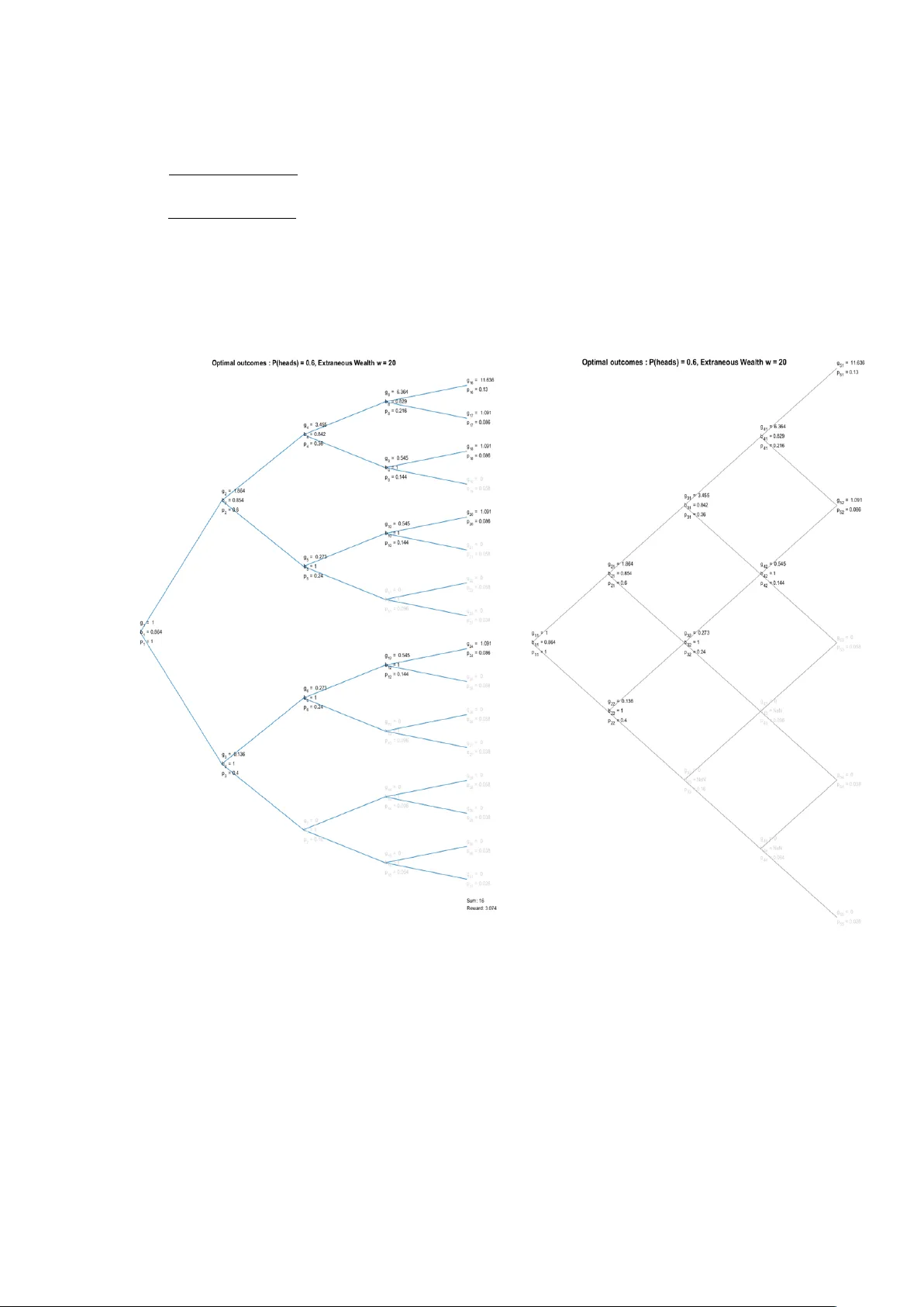
Generalizing the Kelly Strategy Arjun Visw anathan, Head, Rates Big Data, Citibank Global Mark ets Limited (CGML) v4. Dec 5, 2016 Abstract A recen t draft by Victor Haghani and Ric hard Dew ey [1] describ es an exp erimen t where participan ts were giv en initial w ealth, a coin of kno wn bias, and could b et a (v ariable) proportion of their in-game w ealth on a sequence of flips of this coin. Assuming log utilit y and uncapp ed rew ard, the optimal strategy is to b et as per the Kelly criterion. Interestingly , the participan ts in general did not do so - man y b et a larger proportion, up to 100% of their game assets. This note sho ws that suc h b ehaviour can b e rational, if one takes into account the effect of extraneous wealth. The optimal solution for log utilit y with extraneous wealth is found, and extended to the optimal solution for a wide class of utilit y functions. A coun terintuitiv e result is prov ed : for any con tinuous, concav e, differentiable utility function, the optimal choice at every p oint dep ends only on the pr ob ability of re aching that p oint . That is, the optimal choice dep ends only on the numb er of he ads enc ounter e d , regardless of the sequence. Lastly , the practical calculation of the optimal b et at ev ery stage is made p ossible through use of the binomial expansion, reducing the problem size from exp onen tial to quadratic. This makes the solution practical for games with many hundreds of steps. The author thanks Vlad Ragulin 1 , for in tro ducing the original problem, and Andy Morton 2 for motiv ating inv estigation of the general case and economic interpretation of the results. 1 [Director, US Govt Bond T rading, CGML] 2 [Global Head G10 Rates, Markets T reasury and Finance, CGML] 1 1 Setup The pla y er is given 1 unit of game w ealth, and the c hance to b et on f flips of a biased coin coin with kno wn probabilit y p > 0 . 5 of coming up heads. A t ev ery flip, the play er ma y b et a prop ortion b ∈ (0 , 1) of their current game w ealth g on heads. The play er also has extraneous w ealth w , which is not affected b y the b etting. W e initially assume the pla yer’s internal reward function is log utility , i.e. they aim to maximise E [ Log ( g f inal + w )] where g f inal is their final game wealth. If optimizing only one step ahead, the opti- mal bet = (2 p − 1)(1 + w g ) , which reduces to the Kelly betting criterion (2 p − 1) if w = 0. In terestingly , this is not optimal for an n-step game. As one would exp ect, as g  w , the game w ealth dominates and the optimal b et conv erges to (2 p − 1). If g  w , and the game is due to end so on , the optimal b et is 1.00, which agrees with the intuition that there is little downside to b etting the entire tin y stak e. But for moderately long games, the risk of losing paths that could lead to large wealth implies that the first b et m ust b e lo w er than 1. F or example, if p = 0.6 and w = 1000, for 25 flips the optimal first b et is approximately 0.659. 2 Con v enien t notation The p ossible paths of the game form a complete binary tree. W e num b er the no des of this tree with the ro ot = 1. No de n has c hildren No de 2 n (if the coin giv es heads) and Node 2 n + 1(if the coin giv es tails). F or f flips, the final level (that is, level f + 1) has 2 f no des. Let g n = the game w ealth at no de n b n = the b et at no de n p n = the probability of reac hing no de n (1) Figure 1: 2-flip game, p = 0.6, pla y er bets according to the Kelly criterion 2 No de n belongs to lev el b Log 2 ( n ) c +1 , that is F loor [ Log 2 ( n )+1]. A t lev el m, p k ma y tak e m +1 distinct v alues, corresponding to the m + 1 possibilities 0 , 1 , ..., m of the num ber of heads in m flips.Eviden tly g n ≥ 0 for all n . Also g 2 n = g n (1+ b n ) and g 2 n +1 = g n (1- b n ) .This gives us the following recurrences: g n = g 2 n + g 2 n +1 2 b n = g 2 n − g 2 n +1 g 2 n + g 2 n +1 (2) This is useful : if we kno w the final game wealths, we know for free all previous bets and w ealths. 3 Analytic optimal solution for log utilit y & extraneous w ealth Since g 1 = 1 and b y (2) , the unw eigh ted sum of w ealths at level j equals 2 j − 1 W e seek to maximize the total utilit y at the final level P 2 f +1 − 1 k =2 f p k Log ( g k + w ) With additional equality constraint P 2 f +1 − 1 k =2 f g k = 2 f And inequalit y constraint g k ≥ 0 for k = 2 f , 2 f + 1 , ..., 2 f +1 − 1 This is an optimization problem with con v ex and differen tiable ob jective , affine equalit y constraint, and con v ex inequality constraint. Therefore the KKT conditions [2] are necessary and sufficien t to find an optim um. Let x (with 2 f en tries) be the solution of this problem (x is the v ector of final w ealths) In tro ducing Lagrange multipliers λ (a v ector with 2 f en tries) for the inequality constrain t , and ν (a scalar), for the equalit y constraint, we get the standard KKT conditions : x k ≥ 0 , P 2 f k =1 x k = 2 f , λ k ≥ 0 , λ k x k = 0 , and lastly − p k x k + w − λ k + ν = 0 , for k = 1 , 2 , ..., 2 f Usefully , the abov e can directly b e solved for x. Eliminating λ k b et w een the last 2 conditions gives : ( ν − p k x k + w ) x k = 0 and p k x k + w ≤ ν No w suppose ν < p k w . Then p k x k + w ≤ ν < p k w whic h can only o ccur if x k > 0. But then, since ( ν − p k x k + w ) x k = 0 w e must hav e ν = p k x k + w , whic h implies x k = p k ν − w Con versely supp ose ν ≥ p k w . But then x k cannot be strictly greater than zero, for if it was, ( ν − p k x k + w ) x k is the pro duct of tw o terms, b oth strictly greater than 0, and thus cannot b e 0. Therefore w e hav e x k = p k ν − w if p k ν − w > 0, and 0 otherwise, ie x k = max (0 , p k ν − w ) Substituting x k in to the equality constraint, we hav e 3 P 2 f k =1 max (0 , p k ν − w ) = 2 f (3) The LHS of whic h is a strictly decreasing contin uous function of ν ,is zero for large enough ν , and also arbitrarily large if ν is small enough. By the Intermediate V alue Theorem the equation has a unique solution (whic h can b e readily determined, e.g. by binary searc h). Once we hav e ν , w e hav e x , the v ector of optimal final wealths. W e then use (2) to get the opti- mal b ets at every no de. Interestingly , we see that the v alue of x k dep ends only on p k or equiv alen tly the n umber of heads in f flips. This holds in the general case, as is pro ved shortly , which provides a route to efficien t calculation of the best bet at an y p oint. 4 Example F ollo wing the strategy ab ov e for a 4-flip game with p = 0.6, w = 20 would yield the follo wing game tree. P aths where the pla yer b ets all their game wealth and loses are greyed out. Figure 2: 4-flip game, p = 0.6, w = 20, optimal b ets div erge from the Kelly strategy 4 5 Analytic solution for more general utilit y functions W e now consider a general utility function F : R → R , reasonably b e assumed to b e contin uous, concav e and differen tiable. Linear and log utility are sp ecial cases of this type. The deriv ative F 0 need not b e con tinuous, although it is contin uous almost everywhere. F is concav e, therefore F 0 is monotonically decreasing. W e therefore know : F 0 ( w ) ≥ F 0 ( x k + w ). F 0 attains a (not necessarily unique) max at w and a (not neccessarily unique) min at w + 2 f , and if the strict inequalit y F 0 ( w ) > F 0 ( x k + w ) holds then we must hav e x k > 0 W e no w follow exactly the same pro of pattern as before,with F ( x k + w ) and F 0 ( x k + w ) in place of Log ( x k + w ) and 1 x k )+ w As before w e seek to maximize P 2 f +1 − 1 k =2 f p k F ( g k + w ) sub ject to the constraints P 2 f +1 − 1 k =2 f g k = 2 f and g k ≥ 0 for k = 2 f , 2 f + 1 , ..., 2 f +1 − 1 As b efore, introducing Lagrange multipliers λ (a vector with 2 f en tries) for the inequality constrain t, and ν ( a scalar) for the equalit y constrain t, we get the standard KKT conditions : x k ≥ 0 , P 2 f k =1 x k = 2 f , λ k ≥ 0 , λ k x k = 0 , and lastly − p k F 0 ( x k + w ) − λ k + ν = 0 , for k = 1 , 2 , ..., 2 f Eliminating λ k b et w een the last 2 conditions gives : ( − p k F 0 ( x k + w ) + ν ) x k = 0 and p k F 0 ( x k + w ) ≤ ν The first term is the pro duct of tw o nonzero terms. If either is strictly p ositive, the other is zero. As before w e will use this to determine x k . Define the function H as follo ws: H ( y ) = the largest total w ealth z ∈ [ −∞ , w + 2 f ] for which F 0 ( z ) ≥ y H is decreasing and is roughly the inv erse function of the deriv ativ e of the utility: given y , H [ y ] gives a total w ealth ≤ w + 2 f where the marginal utilit y is as close to y as can be without dropping b elow y . Figure 3: illustration of F’ and H, where F is capp ed log utility . 5 No w suppose ν < p k F 0 ( w ) Then p k F 0 ( x k + w ) ≤ ν < p k F 0 ( w ), which can only occur if x k > 0 In this case w e can solve for ν and x k : − p k F 0 ( x k + w ) + ν = 0 ⇒ ν = p k F 0 ( x k + w ) ⇒ x k = H ( ν p k ) − w Secondly suppose ν > p k F 0 ( x k + w ). Then H ( ν p k ) − w m ust be < 0 F or if not, then there exists some z ≥ w for which p k F 0 ( z ) ≥ ν > p k F 0 ( w ), which cannot b e as F 0 is decreasing. So H ( ν p k ) − w < 0 and consequently − p k F 0 ( w ) < ν . But then ν − p k F 0 ( x k + w ) ≥ ν − p k F 0 ( w ) > 0 ⇒ x k = 0 Finally supp ose p k F’(w) = ν , in which case x k migh t b e zero or p ositiv e. Again w e set x k = H ( ν p k ) − w = the largest x k for whic h F 0 ( x k + w ) = F 0 ( w ) (equality holds as F 0 is decreasing). In either case, x k satisfies the KKT conditions. Therefore w e hav e x k = H ( ν p k ) − w if H ( ν p k ) − w > 0 and 0 otherwise, i,e x k = max (0 , H ( ν p k ) − w ) (4) Substituting x k in to the equality constraint, we hav e P 2 f k =1 max (0 , H ( ν p k ) − w ) = 2 f (5) The LHS of which is a decreasing function of ν , and can b e efficien tly solved for ν , e.g. by binary searc h). W e note the symmetry b etw een the ab ov e expressions and the expressions for the optimal so- lution for log utilit y . Once we hav e ν , we hav e x , the vector of optimal final w ealths. W e then use (2) to get the optimal b ets at ev ery no de. 6 Efficien t Calculation There are only f+1 distinct v alues of p k , namely p f , p f − 1 (1 − p ) , ..., (1 − p ) f W e can use the binomial expansion [3] of equation (5) P 2 f k =1 max(0 , H ( ν p k ) − w ) = P f j =0  f j  max (0 , H ( ν p j (1 − p ) f − j ) − w ) = 2 f to calculate ν . This conv enien tly reduces our effort from exp onential to linear to calculate x . Moreo ver, w e can recast our complete binary tree with 2 m no des at level m , into a recombining tree with m nodes at level m . Sp ecifically , if node mn is the n th node at lev el m of the recom bining tree, let g mn , b mn , p mn , be the game wealth at, bet at, and probability of arriving at, node mn . ? 6 Then, b y (2) , we hav e the recurrences g mn = g ( m +1) n + g ( m +1)( n +1) 2 b mn = g ( m +1) n − g ( m +1)( n +1 g ( m +1) n + g ( m +1)( n +1) (6) Eac h lev el of m no des tak es O ( m ) effort to calculate. The full set takes effort O (1 + 2 + ... + f ) = O ( f 2 ) This reduces the effort for the full tree from exp onential to quadratic: Figure 4: Binary and recombining trees 7 The expression for the very first b et has a nice form : if x 0 , x 1 , ...x f are the distinct v alues that the final w ealth can tak e in the r e c ombining tree, the very first bet is 1 2 f f X j =0  f j  f − 2 j f − j x j Whic h ma y b e verified in a v ariet y of wa ys: induction on f, binomial iden tities, generating functions. [3] 7 Conclusion This seems a natural point to pause. This note has generalized the standard Kelly strategy to an optimal strategy for situations with extraneous wealth, and under a muc h more general class of reward functions. The optimal strategy for pathological reward functions e.g. no where differentiable, are left as an ex- ercise to the reader, but are unlik ely to o ccur in reality (one hopes). Of practical v alue is the calculation metho dology which lets us efficien tly deriv e optimal strategies for games of many hundreds or thousands of turns. The biased coin metaphor applies not only to long term in vesting but an y decision pro cess where entities ha v e a notional edge- for example, to help a market making desk create prices more optimally . This metho d might prov e of use in more complex games, e.g. the Halite Artificial Intelligence Chal- lenge at www.halite.io , which shares some k ey similarities with the coinflipping game. The note concludes with an anecdote: A mathematician was aske d by their manager to design a chair. They quickly solve d the pr oblem of a chair with zer o le gs, and with slightly mor e effort, a chair with infinite le gs. A chair with p ositive r e al (though not ne c essarily inte ger) le gs was c onje ctur e d to exist. Final ly, one we ekend, they solve d this variation as wel l, although ne gative le gs r emains an op en pr oblem. References [1] Victor Haghani and Ric hard Dew ey . Rational Decision-Making under Uncertaint y: Observ ed Betting Patterns on a Biased Coin. W orking draft (Octob er 19, 2016). Av ailable at SSRN: h ttps://ssrn.com/abstract=2856963 [2] Stephen Boyd and Liev en V anden berghe. Conv ex Optimization. Cam bridge Univ ersity Press 2004. ISBN 978-0-521-83378-3 [3] Donald Kn uth. The Art of Computer Programming, V olume 1: F undamental Algorithms, Third Edition (Reading, Massach usetts: Addison-W esley , 1997). ISBN 0-201-89683-4 8